Dimensional Synthesis for Multi-Linkage Robots Based on a Niched Pareto Genetic Algorithm

Abstract
1. Introduction
2. Objective Functions of NPGA
2.1. Workspace Density Function
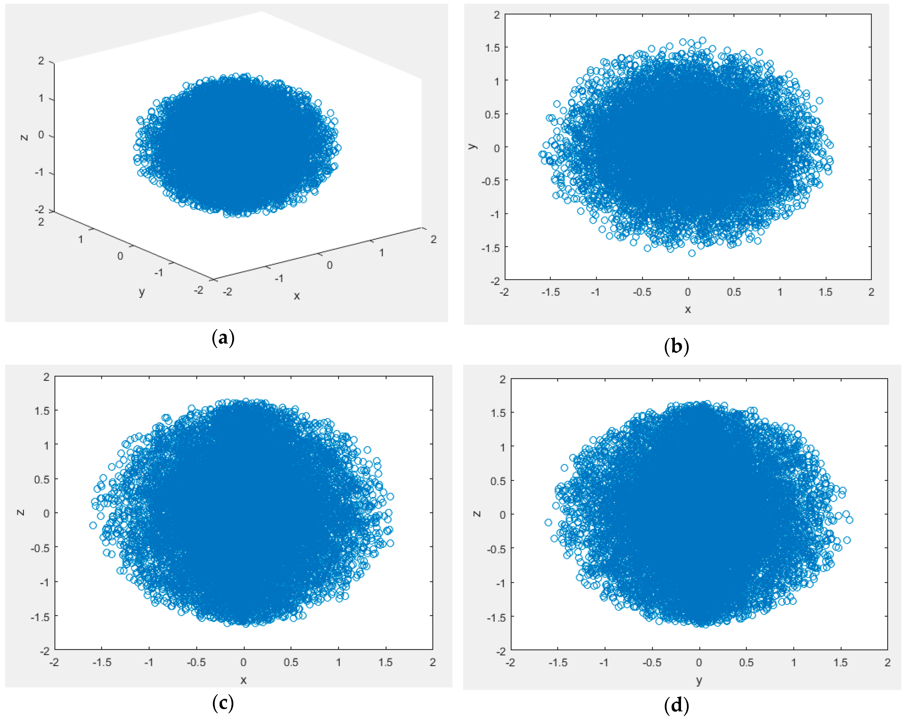
2.1.1. Calculation of Monte Carlo method
- Divide the samples of each joint angle, construct the sample space according to the definition of flexible workspace;
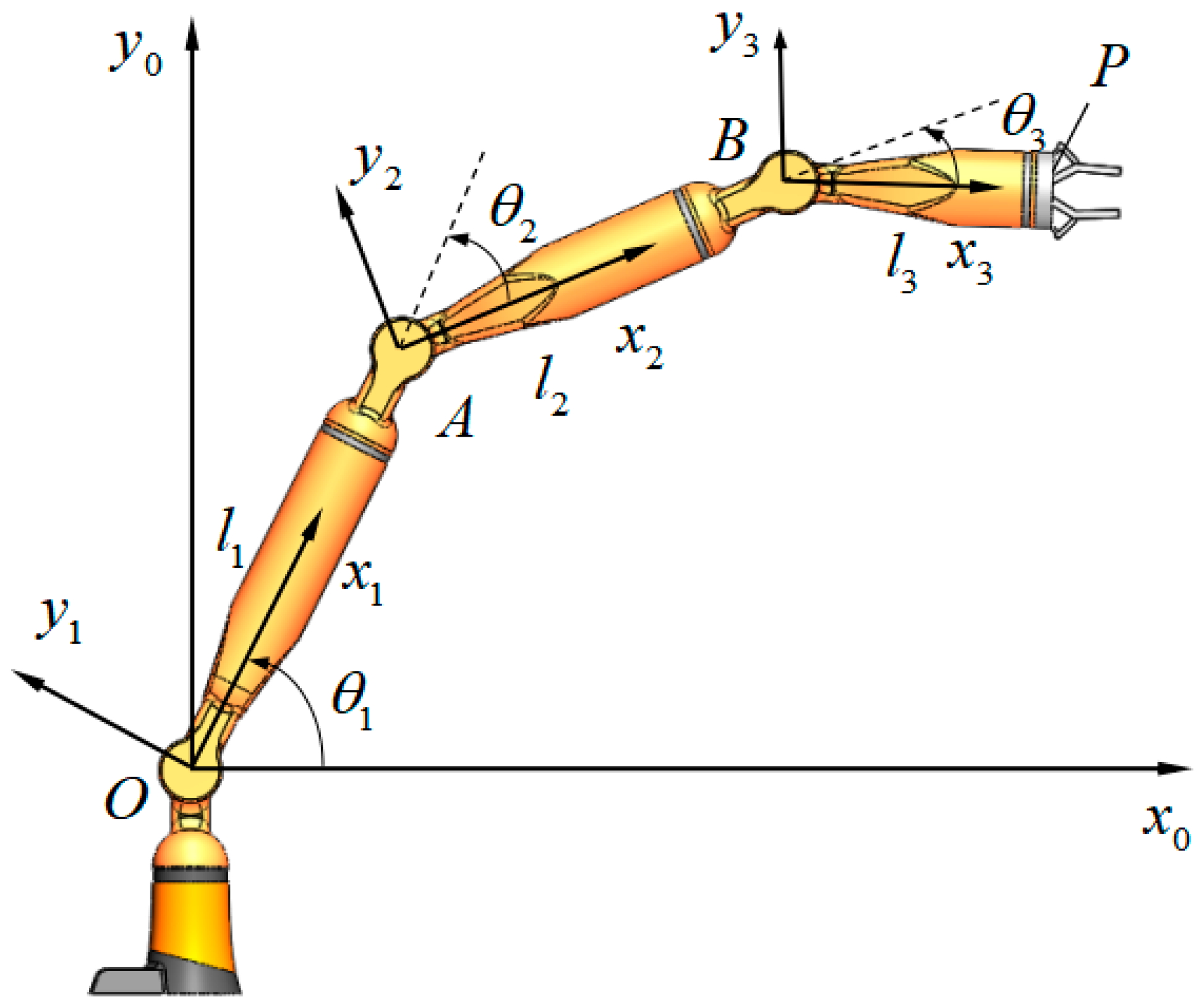
- Calculate the positions end-effector reached on the basis of forward kinematics expression ;
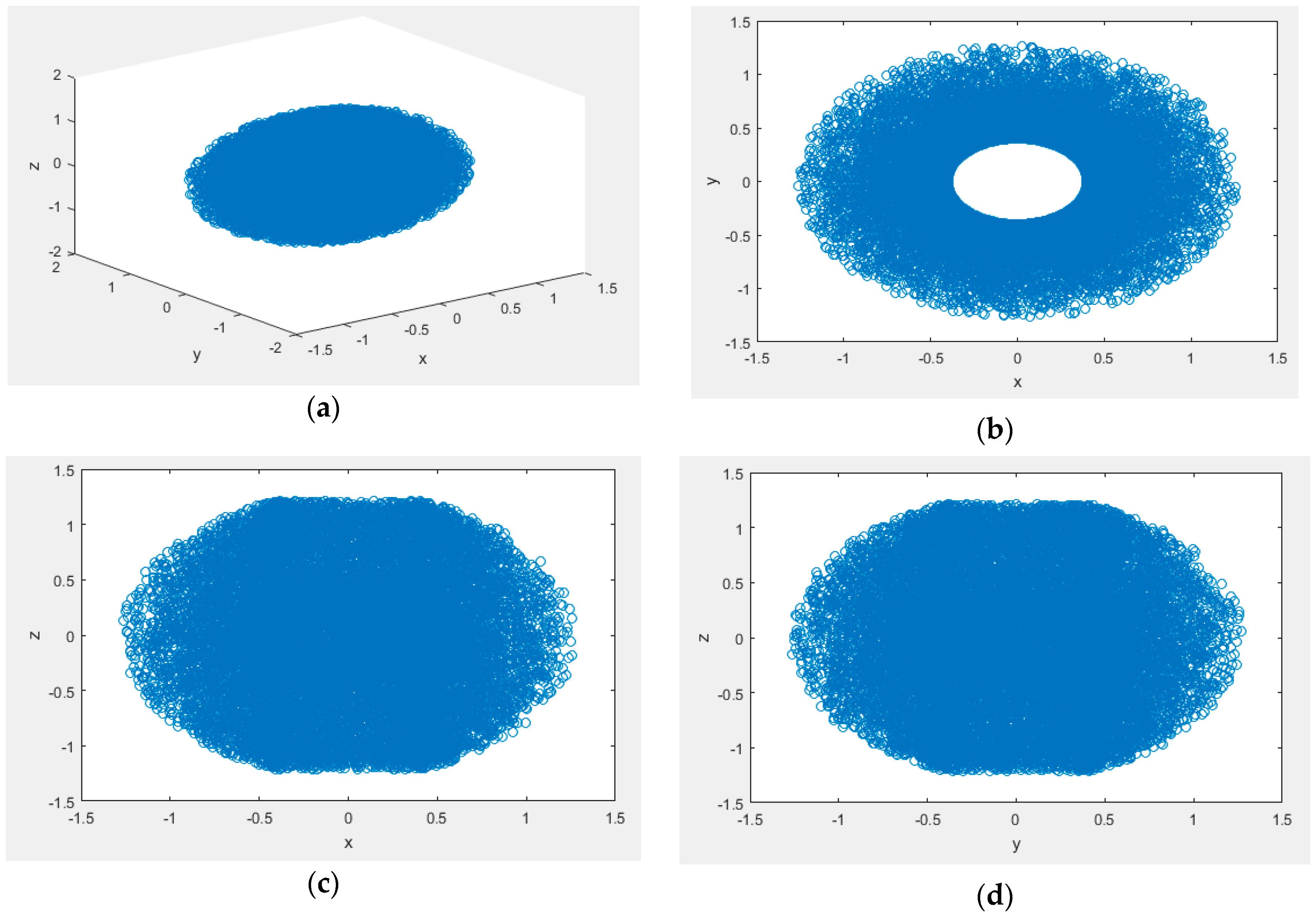
- Construct the flexible workspace using outputted the end-effector position. The larger the sample size, the geometric contour will be clearer and the flexible workspace will be more accurate.
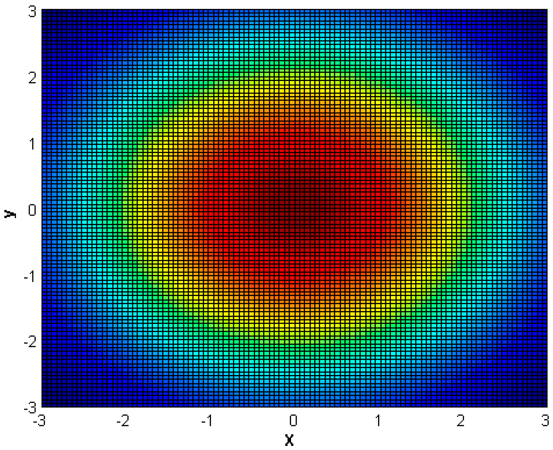
2.1.2. Construction of Density Functions
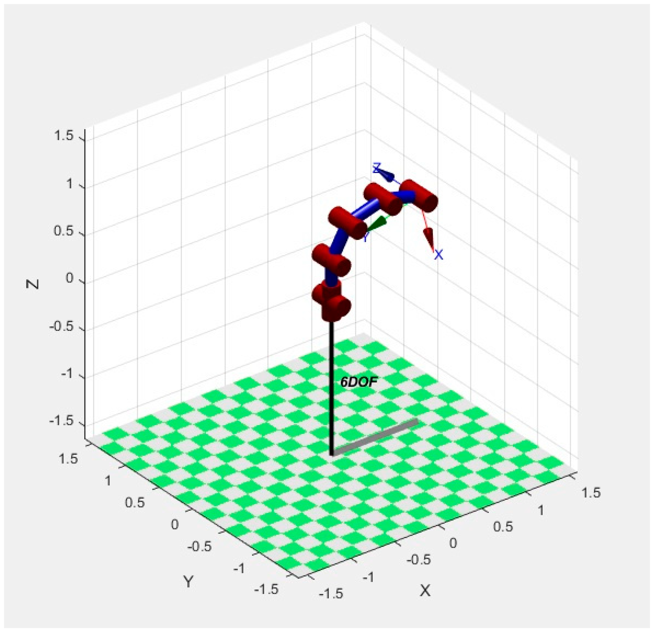
2.1.3. Numerical Example
2.2. Maneuverability
2.3. Energy Expenditure
3. Niche Pareto Genetic Algorithms
3.1. NPGA Sharing Function
3.2. NPGA Fitness
3.3. Design of NPGA
3.3.1. Choice of Coding Method
- The symbol bit is represented by S: 0 is positive, 1 is negative;
- N represents the binary bits of an int;
- The exponent bit is denoted by E;
- Mantissa is represented by M;
3.3.2. Choice of Operators
3.3.3. Choice of Crossover Operator
3.3.4. Choice of Mutation Operator
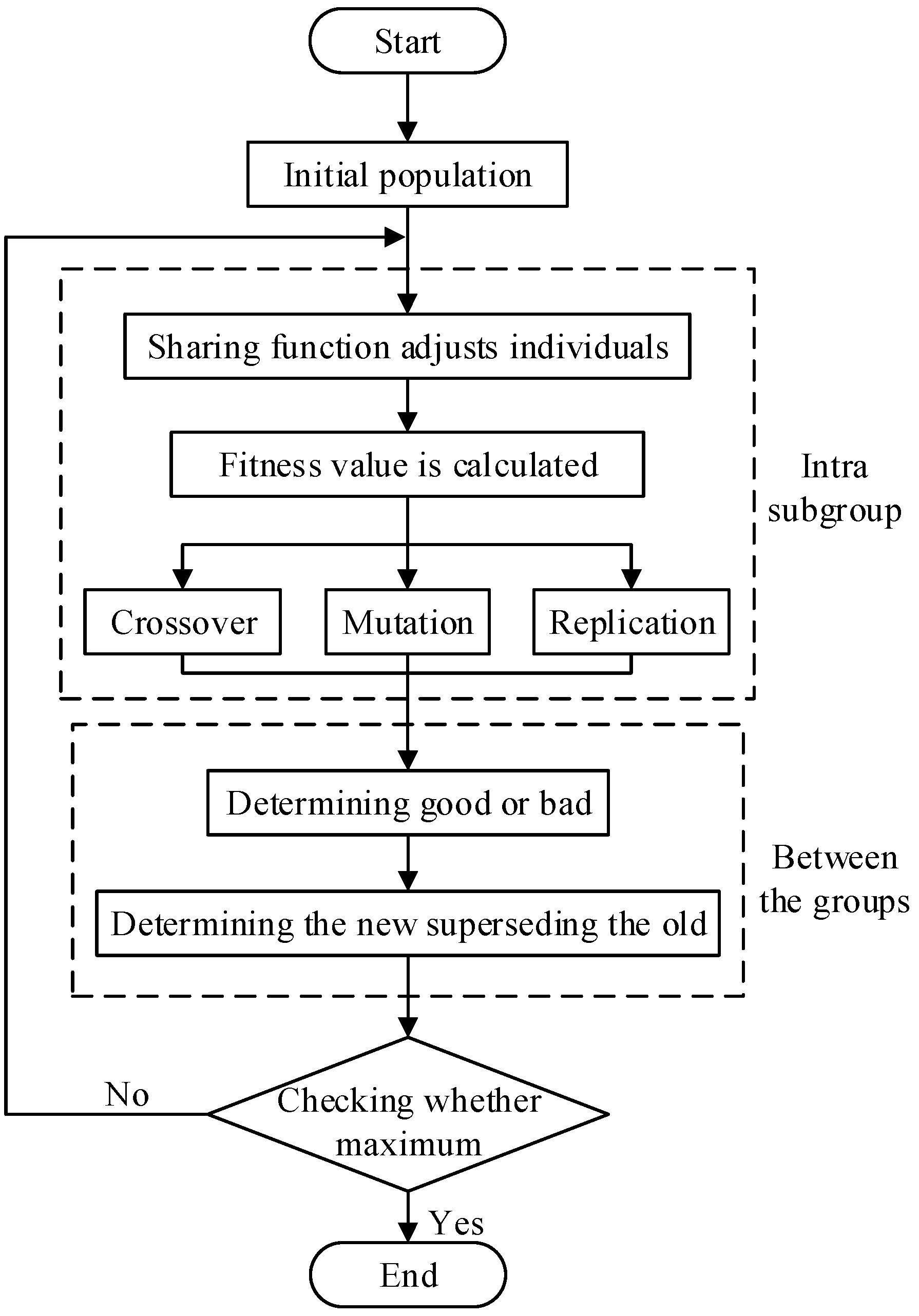
3.3.5. Operation Flow Chart
- Initialization of algorithm, produce new initial population and set up genetic parameters;
- Calculate the sharing degree;
- Calculate individuals’ fitness of population according to the individual sharing;
- Process of selecting, crossing, and mutating;
- Comparing of fitness size between offspring and last generation individuals;
- Offspring replace last generation individuals, forming a new population;
- The algorithm stops until the termination condition is activated, otherwise go back to Step 2.
4. Mathematical Model of Dimensional Synthesis
5. Engineering Example of the Method Application and Analysis
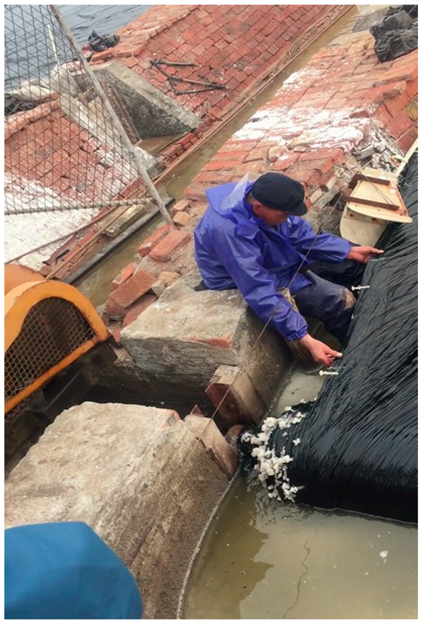
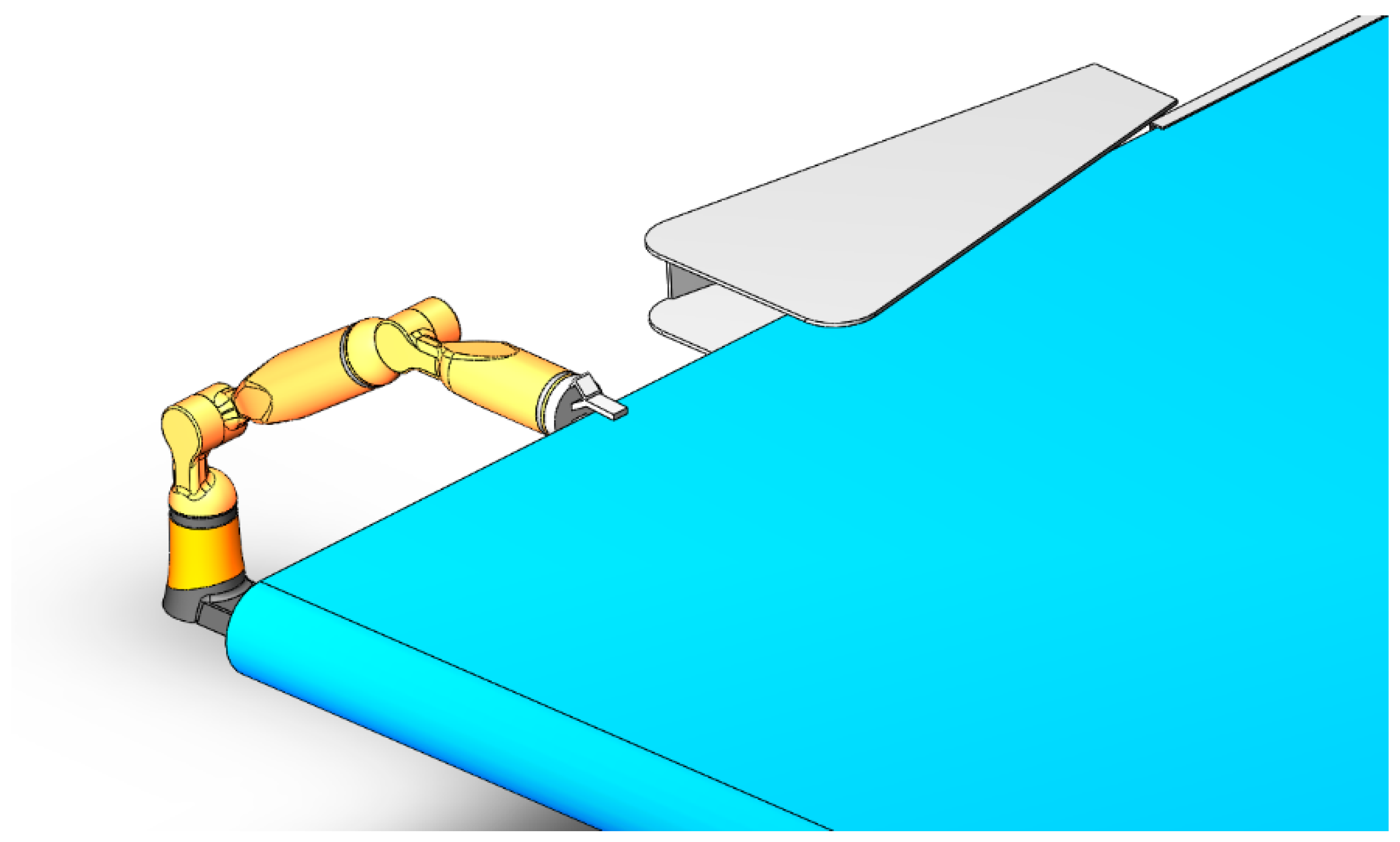
5.1. Method Application in Salt Industry
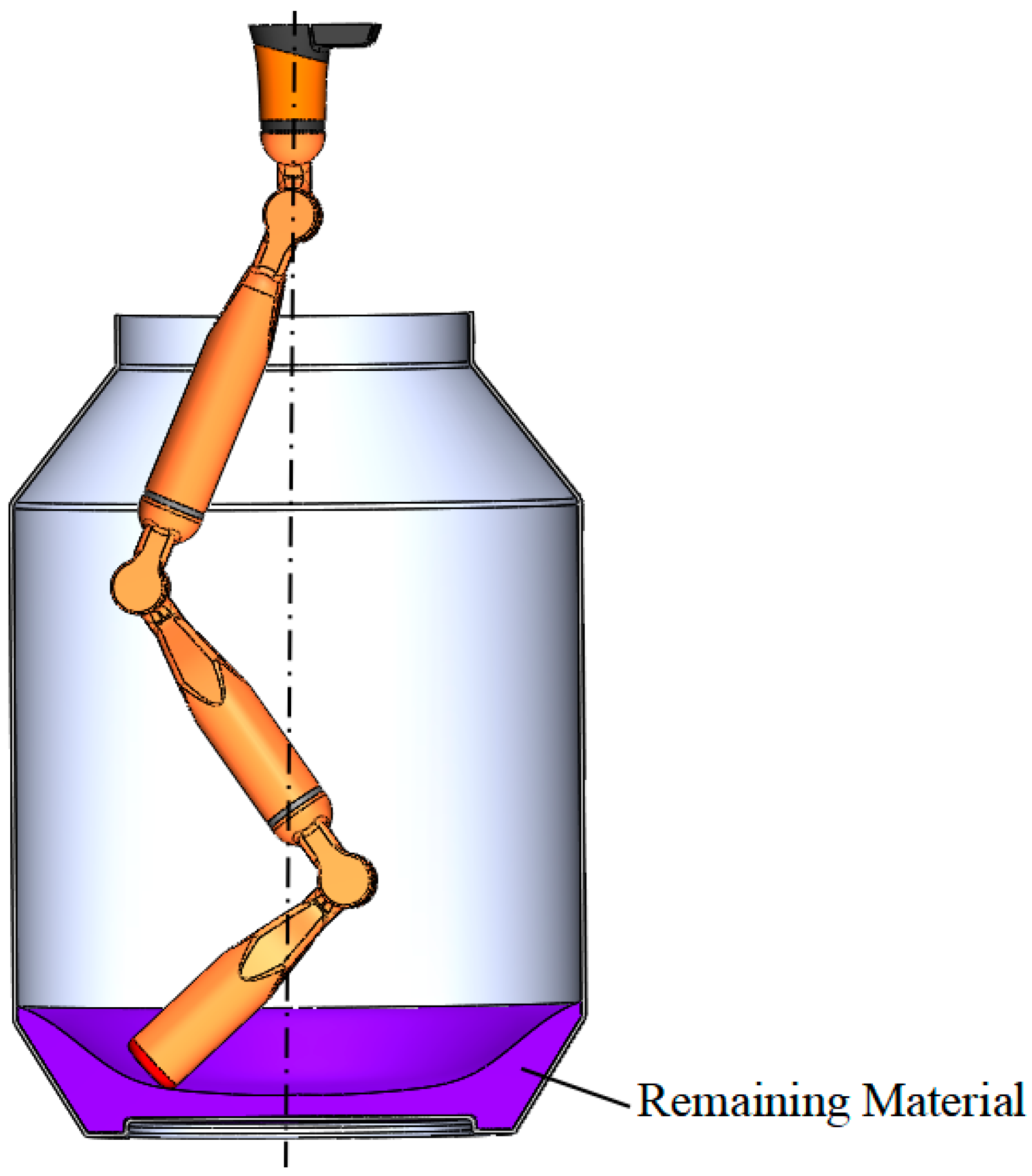
5.2. Method Application in Chemical Industry
6. Conclusions
- Based on the study of workspace, maneuverability, and energy expenditure, the NPGA method for dimensional synthesis of multi-linkage robot was proposed and applied. Then, the NPGA was applied;
- The superiority of NPGA method was verified by comparing with the KPCA method in two applications. The study provided new ideas and methods for the salt field’s unmanned mechanized production and design of hazardous chemical processing equipment;
- For the method of dimensional synthesis of multi-linkage robots, it is possible to obtain a locally convergent solution set under a special environment and specific constraint conditions, but the Pareto solution set with global convergence cannot be obtained. It is possible to obtain a locally convergent solution set, and the algorithm needs to be further improved.
Author Contributions
Funding
Acknowledgments
Conflicts of Interest
References
- Lv, B.H. Research on Key Technology of Multi Degrees of Freedom Dexterous Hand for Space Robot. Beijing. Master’s Thesis, The First Academy of China Aerospace Science and Technology Corporation, Beijing, China, 2019. [Google Scholar]
- Huang, A.; Yao, D.; Yang, W.; Zhang, G.; Li, Y. Kinematics and Dexterity Analysis of Mobile Manipulator. Mod. Manuf. Technol. Equip. 2019, 7, 28–31. [Google Scholar]
- Gosselin, C.; Angeles, J. A Global Performance Index for the Kinematic Optimization of Robotic Manipulators. ASME J. Mech. Des. 1991, 113, 220–226. [Google Scholar] [CrossRef]
- Dastjerdi, A.H.; Sheikhi, M.M.; Masouleh, M.T. A Complete Analytical Solution for the Dimensional Synthesis of 3-DOF Delta Parallel Robot for a Prescribed Workspace. Mech. Mach. Theory 2020, 153, 103991. [Google Scholar] [CrossRef]
- Leal-Naranjo, J.A.; Soria-Alcaraz, J.A.; Torres-San Miguel, C.R.; Paredes-Rojas, J.C.; Espinal, A.; Rostro-González, H. Comparison of Metaheuristic Optimization Algorithms for Dimensional Synthesis of a Spherical Parallel Manipulator. Mech. Mach. Theory 2019, 140, 586–600. [Google Scholar] [CrossRef]
- Sancibrian, R.; Sedano, A.; Esther, G.S.; Jesus, M.B. Hybridizing differential evolution and local search optimization for dimensional synthesis of linkages. Mech. Mach. Theory 2019, 140, 389–412. [Google Scholar] [CrossRef]
- Jia, S.; Jia, Y.; Xu, S. Dimensional Optimization Method for Manipulator Based on Orientation Manipulability. J. Beijing Univ. Aeronaut. Astronaut. 2015, 41, 1693–1700. [Google Scholar]
- Zhao, K.; Fu, Y.; Niu, G.; Pan, B. Mechanical Design and Dimensional Optimization of Minimally Invasive Celiac Surgical Robot. Huazhong. Univ. Sci. Tech. (Nat. Sci. Ed.) 2013, 41, 324–328. [Google Scholar]
- Ma, G.Q. Structure Design and Optimization Research of Mechanical Arm of Mobile Service Robot. Master’s Thesis, Harbin Institute of Technology, Harbin, China, 2014. [Google Scholar]
- Surbhi, G.; Sankho, T.S.; Amod, K. Design Optimization of Minimally Invasive Surgical Robot. Appl. Soft Comput. 2015, 32, 241–249. [Google Scholar]
- Dong, H.; Wu, W.T.; Sun, H. Dimension Optimization of Manipulator Based on Workspace Density Function. Mach. Build. Autom. 2019, 36, 143–146. [Google Scholar]
- Wang, S.; Wang, X.; Zhang, J. A New Robot to Assist Minimally Invasive Abdominal Surgery. Robot. Tech. Appl. 2011, 4, 6–11. [Google Scholar]
- Wu, Y.; Tang, X.; Song, W.; Jiang, P.; Zhou, J.; Chen, Y. Power Equivalent Model of Industrial Robot and Parameter Identification. J. Chongqing Univ. 1–13. Available online: https://kns.cnki.net/kcms/detail/50.1044.N.20200610.1138.002.html (accessed on 10 June 2020). (In Chinese).
- Jing, X.; Xue, Y.; Chen, Y. Analysis and Parameters Optimization of 6R Dual-Arm Service Robot Collaborative Space. Mech. Sci. Technol. Aerosp. Eng. 1–6. Available online: https://kns.cnki.net/kcms/detail/61.1114.TH.20200707.1003.003.html (accessed on 7 July 2020). (In Chinese).
- Zhang, L.; Tang, K.; Zhao, Y.; Wang, X.; Yu, D.; Lu, X.; Wang, X. Optimization of Leg Structure Parameter of Quadruped Laser Weeding Robot. Trans. Chin. Soc. Agric. Eng. (Trans. CSAE) 2020, 36, 7–15. [Google Scholar] [CrossRef]
- Wang, L.; Wang, C.; Du, W.; Xie, G.Z.; Song, K.K.; Wang, X.J.; Zhao, F. Parameter Optimization of a Four-Legged Robot to Improve Motion Trajectory Accuracy Using Signal-to-Noise Ratio Theory. Robot. Comput.-Integr. Manuf. 2018, 51, 85–96. [Google Scholar] [CrossRef]
- Feng, H.; Miao, Q.; Fan, S.; Wang, H.L.; Wang, W. Modular and Parametric Design for Mechanical Structure of Industrial Robots. Mach. Tool. Hydraul. 2019, 47, 60–63. [Google Scholar]
- Chen, J.X. Mechanism Design and Parameter Calculation of a New Crawling Robot. Mod. Manuf. Technol. Equip. 2019, 271, 76–77. [Google Scholar]
- Gao, W.; Liu, M.; Zhang, J.; Zhang, H. Structure Analysis and Optimization of Manipulator’s Structure of the Robotic Explorer in Nuclear Environment. Mach. Des. Manuf. 2020, 5, 245–252. [Google Scholar]
- Xiao, X.; Fang, Y. Design and Optimization of Hydraulic-Driven Coal Mine Rescue Wheeled Robot. Mach. Des. Manuf. 2020, 3, 265–268. [Google Scholar]
- Dong, H. Kinematics of Rdundant Manipulator and Dead-Reckoning and Path Planning Research of Mobile Platform. Master’s Thesis, Harbin Institute of Technology, Harbin, China, 2015. [Google Scholar]
- Ye, C.; Mao, Z.; Liu, M. A Novel Multi-Objective Five-Elements Cycle Optimization Algorithm. Algorithm 2019, 12, 244. [Google Scholar] [CrossRef]
- Xiao, Y.; Hua, Z. Misalignment Fault Prediction of Wind Turbines Based on Combined Forecasting Model. Algorithm 2020, 13, 56. [Google Scholar] [CrossRef]
- Alekseeva, N.; Tanev, I.; Shimohara, K. PD Steering Controller Utilizing the Predicted Position on Track for Autonomous Vehicles Driven on Slippery Roads. Algorithm 2020, 13, 48. [Google Scholar] [CrossRef]
- Sai, Q.; Bi, J.; Chai, J. Optimal Model for Carsharing Station Location Based on Multi-Factor Constraints. Algorithm 2020, 13, 43. [Google Scholar] [CrossRef]
- Xie, B.; Jing, Z. Advances in Robotic Kinematic Dexterity and Indices. Mech. Sci. Technol. Aerosp. Eng. 2011, 30, 1386–1393. [Google Scholar]
- Xie, B.; Jing, Z. Directional Manipulability Constrained by the Condition Number. J. Mech. Eng. 2010, 46, 8–15. [Google Scholar] [CrossRef]
- Zhang, P.; Yao, Z.Q.; Du, Z.C. Global Performance Index System for Kinematic Optimization of Robotic Mechanism. ASME J. Mech. Des. 2014, 136, 1–11. [Google Scholar] [CrossRef]
- Dong, H.; Du, Z. Obstacle Avoidance Path Planning of Planar Redundant Manipulators using Workspace Density. Int. J. Adv. Robot. Syst. 2014, 12, 1–10. [Google Scholar] [CrossRef]
- Yoshikawa, T. Manipulability of robotic mechanism. Int. J. Robot. Res. 1985, 4, 3–9. [Google Scholar] [CrossRef]
- Jose, S.; Vijayalakshmi, C. Design and Analysis of Multi-Objective Optimization Problem Using Evolutionary Algorithms. Procedia Comput. Sci. 2020, 172, 896–899. [Google Scholar] [CrossRef]
- Martín, D.; Alcalá-Fdez, J.; Rosete, A.; Herrera, F. NICGAR: A Niching Genetic Algorithm to Mine a Diverse Set of Interesting Quantitative Association Rules. Inf. Sci. 2016, 355, 208–228. [Google Scholar] [CrossRef]
- Sun, Z.; Zhao, J.; Li, L. Application of Simultaneous Mechanism Analysis and Synthesisin Serial Robots. J. Beijing Univ. Technol. 2014, 3, 321–327. [Google Scholar]


| Links | ||||
|---|---|---|---|---|
| Team1 | 12.1661 | 15.8215 | 0.5923 | 2.0844 |
| Team2 | 11.9238 | 16.0003 | 0.6235 | 2.0936 |
| Team3 | 11.9806 | 16.1216 | 0.6345 | 1.9962 |
| Team4 | 12.0201 | 15.9944 | 0.5812 | 1.8796 |
| Team5 | 11.0569 | 16.1725 | 0.5771 | 1.9236 |
| Team6 | 11.9754 | 16.0258 | 0.6121 | 2.0612 |
| Team7 | 11.8962 | 16.3501 | 0.5956 | 2..1003 |
| Team8 | 12.0821 | 15.9812 | 0.6135 | 2.0732 |
| Links | ||||
|---|---|---|---|---|
| Team1 | 11.0361 | 17.0021 | 0.5756 | 2.0311 |
| Team2 | 10.9512 | 16.8802 | 0.5608 | 2.1051 |
| Team3 | 11.1004 | 16.7560 | 0.5732 | 1.9601 |
| Team4 | 10.9913 | 17.0103 | 0.5714 | 1.9985 |
| Team5 | 11.0032 | 17.1022 | 0.5746 | 2.5543 |
| Team6 | 10.8239 | 16.9823 | 0.5611 | 1.9723 |
| Team7 | 10.9025 | 17.1005 | 0.5802 | 1.9028 |
| Team8 | 11.0344 | 16.9562 | 0.5913 | 2.0048 |
| Design Method | Joint Angle | Elapsed Time |
|---|---|---|
| KPCA | ||
| NPGA |
| Links | ||||||
|---|---|---|---|---|---|---|
| Team1 | 15.1023 | 23.1212 | 25.1223 | 1.1684 | 1.6863 | 2.0615 |
| Team2 | 14.8623 | 23.0258 | 25.0782 | 1.1697 | 1.6912 | 2.1109 |
| Team3 | 14.7956 | 23.1203 | 24.9036 | 1.1716 | 1.7065 | 2.0738 |
| Team4 | 15.0023 | 22.7250 | 24.9956 | 1.1702 | 1.6544 | 2.0752 |
| Team5 | 15.0320 | 22.8155 | 24.7152 | 1.1686 | 1.6764 | 2.0813 |
| Team6 | 15.1780 | 23.2013 | 24.8574 | 1.1581 | 1.7106 | 2.1024 |
| Team7 | 15.2311 | 23.0035 | 25.1129 | 1.1573 | 1.6872 | 2.0623 |
| Team8 | 14.9055 | 23.1322 | 25.3001 | 1.1592 | 1.6928 | 2.0668 |
| Links | ||||||
|---|---|---|---|---|---|---|
| Team1 | 16.0521 | 22.3212 | 26.1001 | 1.1389 | 1.6530 | 2.0411 |
| Team2 | 16.0518 | 21.0258 | 25.9688 | 1.1370 | 1.6747 | 2.0418 |
| Team3 | 16.1325 | 23.0004 | 26.3803 | 1.1424 | 1.5985 | 2.0652 |
| Team4 | 15.9921 | 22.3250 | 25.9975 | 1.1560 | 1.5980 | 2.1001 |
| Team5 | 16.0039 | 22.1022 | 26.1023 | 1.1325 | 1.5543 | 2.0365 |
| Team6 | 16.0233 | 21.9867 | 26.1104 | 1.1335 | 1.5921 | 2.0402 |
| Team7 | 15.9936 | 22.7560 | 26.3622 | 1.1338 | 1.6023 | 2.0466 |
| Team8 | 16.0365 | 22.0053 | 26.4510 | 1.1381 | 1.6684 | 2.0439 |
| Design Method | Joint Angle | Elapsed Time |
|---|---|---|
| KPCA | ||
| NPGA |
© 2020 by the authors. Licensee MDPI, Basel, Switzerland. This article is an open access article distributed under the terms and conditions of the Creative Commons Attribution (CC BY) license (http://creativecommons.org/licenses/by/4.0/).
Share and Cite
Wu, H.; Li, X.; Yang, X. Dimensional Synthesis for Multi-Linkage Robots Based on a Niched Pareto Genetic Algorithm. Algorithms 2020, 13, 203. https://doi.org/10.3390/a13090203
Wu H, Li X, Yang X. Dimensional Synthesis for Multi-Linkage Robots Based on a Niched Pareto Genetic Algorithm. Algorithms. 2020; 13(9):203. https://doi.org/10.3390/a13090203
Chicago/Turabian StyleWu, Hu, Xinning Li, and Xianhai Yang. 2020. "Dimensional Synthesis for Multi-Linkage Robots Based on a Niched Pareto Genetic Algorithm" Algorithms 13, no. 9: 203. https://doi.org/10.3390/a13090203
APA StyleWu, H., Li, X., & Yang, X. (2020). Dimensional Synthesis for Multi-Linkage Robots Based on a Niched Pareto Genetic Algorithm. Algorithms, 13(9), 203. https://doi.org/10.3390/a13090203