Finding the Best 3-OPT Move in Subcubic Time

Abstract

Given a Traveling Salesman Problem solution, the best 3-OPT move requires us to remove three edges and replace them with three new ones so as to shorten the tour as much as possible. No worst-case algorithm better than the $\mathsf{\Theta }\left(n^3\right)$ enumeration of all triples is likely to exist for this problem, but algorithms with average case $O\left(n^{3-ϵ}\right)$ are not ruled out. In this paper we describe a strategy for 3-OPT optimization which can find the best move by looking only at a fraction of all possible moves. We extend our approach also to some other types of cubic moves, such as some special 6-OPT and 5-OPT moves. Empirical evidence shows that our algorithm runs in average subcubic time (upper bounded by $O\left(n^{2.5}\right)$) on a wide class of random graphs as well as Traveling Salesman Problem Library (TSPLIB) instances.

1. Introduction

The Traveling Salesman Problem (TSP), in all likelihood the most famous combinatorial optimization problem, calls for finding the shortest Hamiltonian cycle in a complete graph $G=(V,E)$ of n nodes, weighted on the arcs. In this paper we consider the symmetric TSP, i.e., the graph is undirected and the distance between two nodes is the same irrespective of the direction in which we traverse an edge. Let us denote by $c(i,j)=c(j,i)$ the distance between any two nodes i and j. We call each solution of the problem a tour. A tour is identified by a permutation of vertices $(v_1,\dots ,v_n)$. We call $\{v_i,v_{i+1}\}$, for $i=1,\dots ,n-1$, and $\{v_n,v_1\}$ the edges of the tour. The length of a tour T, denoted by $c\left(T\right)$ is the sum of the lengths of the edges of the tour. More generally, for any set F of edges, we denote by $c\left(F\right)$ the value ${\sum }_{e\in F}c\left(e\right)$.

A large number of applications over the years have shown that local search is often a very effective way to tackle hard combinatorial optimization problems, including the TSP. The local search paradigm applies to a generic optimization problem in which we seek to minimize an objective function $f\left(x\right)$ over a set X. Given a map $N:X\mapsto 2^X$ which associates to every solution $x\in X$ a set $N\left(x\right)$ called its neighborhood, the basic idea is the following: start at any solution $x^0$, set $s:=x^0$, and look for a solution $x^1\in N\left(s\right)$ better than s. If we find one, we replace s with $x^1$ and iterate the same search. We continue this way until we get to a solution s such that $f\left(s\right)=min\left\{f\right(x\left)\right|x\in N\left(s\right)\}$. In this case, we say that s is a local optimum. Replacing $x^i$ with $x^{i+1}$ is called performing a move of the search, and $N\left(s\right)$ is the set of all solutions reachable with a move from s. The total number of moves performed to get from $x^0$ to the final local optimum is called the length of the convergence. If x is a solution reachable with a move from s and $f\left(x\right)<f\left(s\right)$ we say that the move is an improving move and x is an improving solution. When searching in the neighborhood of $x^i$ we can adopt two main strategies, namely first-improvement and best-improvement (also called steepest-descent). In the first-improvement strategy, we set $x^{i+1}$ to be the first solution that we find in $N\left(x^i\right)$ such that $f\left(x^{i+1}\right)<f\left(x^i\right)$. In best-improvement, we set $x^{i+1}$ to be such that $f\left(x^{i+1}\right)=min\left\{f\left(x\right)\right|x\in N\left(x^i\right)\wedge f\left(x\right)<f\left(x^i\right)\}$. For small-size neighborhoods such as the one considered in this paper, most local search procedures choose to adopt the best-improvement strategy, since it causes the largest decrease in the objective function value at any given iteration of the search. In this paper we will focus precisely on the objective of finding the best possible move for a popular TSP neighborhood, i.e., the 3-OPT.

The idea of basic local search has been around for a very long time and it is difficult to attribute it to any particular author. Examples of its use are reported in standard textbooks on combinatorial optimization, such as [1], or devoted surveys, such as [2]. In time, many variants have been proposed to make local search more effective by avoiding it to get stuck in local optima. Namely, sometimes a non-improving move must be performed to keep the search going. Examples of these techniques are tabu search [3] and simulated annealing [4]. Our results apply to basic local search but can be readily adapted to use in more sophisticated procedures such as tabu search. This, however, is beyond the scope of this paper.

1.1. The K-OPT Neighborhood

Let $K\in \mathbb{N}$ be a constant. A K-OPT move on a tour T consists of first removing a set R of K edges and then inserting a set I of K edges so as $(T\backslash R)\cup I$ is still a tour (we include, possibly, $R\cap I\ne \varnothing$. This implies that the $(K-1)$-OPT moves are a subset of the K-OPT moves). A K-OPT move is improving if $c\left(\right(T\backslash R)\cup I)<c\left(T\right)$ i.e., $c\left(I\right)<c\left(R\right)$. An improving move is best improving if $c\left(R\right)-c\left(I\right)$ is the maximum over all possible choices of $R,I$.

The standard local search approach for the TSP based on the K-OPT neighborhood starts from any tour $T^0$ (usually a random permutation of the vertices) and then proceeds along a sequence of tours $T^1,T^2,\dots ,T^N$ where each tour $T^j$ is obtained by applying an improving K-OPT move to $T^{j-1}$. The final tour $T^N$ is such that there are no improving K-OPT moves for it. The hope is that $T^N$ is a good tour (optimistically, a global optimum) but its quality depends on many factors. One of them is the size of the neighborhood, the rationale being that with a larger-size neighborhood we sample a larger number of potential solutions, and hence increase the probability of ending up at a really good one. Clearly, there is a trade-off between the size of a neighborhood and the time required to explore it, so that most times people resort to the use of small neighborhoods since they are very fast to explore (for a discussion on how to deal with some very large size, i.e., exponential, neighborhoods for various combinatorial optimization problems, see [5]).

The exploration of the K-OPT neighborhood, for a fixed K, might be considered “fast” from a theoretical point of view, since there is an obvious polynomial algorithm (complete enumeration). However, in practice, complete enumeration makes the use of K-OPT impossible already for $K=3$ (if n is large enough, like 3000 or more). There are $\mathsf{\Theta }\left(n^K\right)$ choices of K edges to remove which implies that 3-OPT can be explored in time $O\left(n^3\right)$ by listing all possibilities. For a given tour $n=6000$ nodes, the time required to try all 3-OPT moves, on a reasonably fast desktop computer, is more than one hour, let alone converging to a local optimum. For this reason, 3-OPT has never been really adopted for the heuristic solution of the TSP.

The first use of K-OPT dates back to 1958 with the introduction of 2-OPT for the solution of the TSP in [6]. In 1965 Lin [7] described the 3-OPT neighborhood, and experimented with the $\mathsf{\Theta }\left(n^3\right)$ algorithm, on which he also introduced a heuristic step fixing some edges of the solution (at risk of being wrong) with the goal of decreasing the size of the instance. Still, the instances which could be tackled at the time were fairly small ($n\le 150$). Later in 1968, Steiglitz and Weiner [8] described an improvement over Lin’s method which made it 2 or 3 times faster, but still cubic in nature.

It was soon realized that the case $K\ge 3$ was impractical, and later local search heuristics deviated from the paradigm of complete exploration of the neighborhood, replacing it with some clever ways to heuristically move from tour to tour. The best such heuristic is probably Lin and Kernighan’s procedure [9] which applies a sequence of K-OPT moves for different values of K. Notice that our objective, and our approach, is fundamentally different from Lin and Kernighan’s in that we always look for the best K-OPT move, and we keep K constantly equal to 3. On the other hand, Lin and Kernighan, besides varying K, apply a heuristic search for the best K-OPT move, which is fast but cannot guarantee to find the best move, and, indeed, is not guaranteed to find an improving move even if some exist. For a very good chapter comparing various heuristics for the TSP, including the 3-OPT neighborhood, see Johnson and Mc Geich [10].

An important recent result in [11] proves that, under a widely believed hypothesis similar to the $P\ne NP$ conjecture, it is impossible to find the best 3-OPT move with a worst-case algorithm of time $O\left(n^{3-ϵ}\right)$ for any $ϵ>0$ so that complete enumeration is, in a sense, optimal. However, this gives us little consolation when we are faced with the problem of applying 3-OPT to a large TSP instance. In fact, for complete enumeration the average case and the worst case coincide, and one might wonder if there exists a better practical algorithm, much faster than complete enumeration on the majority of instances but still $O\left(n^3\right)$ in the worst case. The algorithm described in this paper (of which a preliminary version appeared in [12]) is such an example. A similar goal, but for problems other than the TSP, is pursued in [13], which focuses on the alternatives to brute force exploration of polynomial-size neighborhoods from the point of view of parameterized complexity.

1.2. The Goal of This Paper

The TSP is today very effectively solved, even to optimality, by using sophisticated mathematical programming-based approaches, such as Concorde [14]. No matter how ingenious, heuristics can hardly be competitive with these approaches when the latter are given enough running time. It is clear that simple heuristics, such as local search, are even less effective.

However, simple heuristics have a great quality which lies in their very name: since they are simple (in all respects, to understand, to implement and to maintain), they are appealing, especially to the world of practical, real-life application solvers, i.e., in the industrial world where the very vast majority of in-house built procedures are of heuristic nature. Besides its simplicity, local search has usually another great appeal: it is in general very fast, so that it can overcome its simplemindedness by the fact that it is able to sample a huge amount of good solutions (the local optima) in a relatively small time. Of course, if its speed is too slow, one loses all the interest in using a local search approach despite its simplicity.

This is exactly the situation for the 3-OPT local search. It is simple, and might be effective, but we cannot use it in practice for mid-to-large sized instances because it is too slow. The goal of our work has been to show that, with a clever implementation of the search for improving moves, it can be actually used since it becomes much faster (even $1000\times$ on the instances we tried) with respect to its standard implementation.

We remark that our intention in this paper is not that of proving that steepest-descent 3-OPT is indeed an effective heuristics for the TSP (this would require a separate work with a lot of experiments and can be the subject of future research). Our goal is to show anyone who is interested in using such a neighborhood how to implement its exploration so as to achieve a huge reductions in the running times. While a full discussion of the computational results can be found in Section 5, here is an example of the type of results that we will achieve with our approach: on a graph of 1000 nodes, we can sample about 100 local optima in the same time that the enumerative approach would take to reach only one local optimum.

2. Selections, Schemes and Moves

Let $G=(V,E)$ be a complete graph on n nodes, and $c:E\mapsto {\mathbb{R}}^{+}$ be a cost function for the edges. Without loss of generality, we assume $V=\{0,1,\dots ,\overline{n}\}$, where $\overline{n}=n-1$. In this paper, we will describe an effective strategy for finding either the best improving or any improving move for a given current tour $(v_1,\dots ,v_n)$. Without loss of generality, we will always assume that the current tour T is the tour

$$(0,1,\dots ,\overline{n}).$$

We will be using modular arithmetic frequently. For convenience, for each $x\in V$ and $t\in \mathbb{N}$ we define

$$x\oplus t:=(x+t)modn,x\ominus t:=(x-t)modn.$$

When moving from x to $x\oplus 1,x\oplus 2$ etc. we say that we are moving clockwise, or forward. In going from x to $x\ominus 1,x\ominus 2,\dots$ we say that we are moving counter-clockwise, or backward.

We define the forward distance $d^{+}(x,y)$ from node x to node y as the $t\in \{0,\dots ,n-1\}$ such that $x\oplus t=y$. Similarly, we define the backward distance $d^{-}(x,y)$ from x to y as the $t\in \{0,\dots ,n-1\}$ such that $x\ominus t=y$. Finally, the distance between any two nodes x and y is defined by

$$d(x,y):=min\{d^{+}(x,y),d^{-}(x,y)\}.$$

A 3-OPT move is fully specified by two sets, i.e., the set of removed and of inserted edges. We call a removal set any set of three tour edges, i.e., three edges of type $\{i,i\oplus 1\}$. A removal set is identified by a triple $S=(i_1,i_2,i_3)$ with $0\le i_1<i_2<i_3\le \overline{n}$, where the edges removed are $R\left(S\right):=\{\{i_j,i_j\oplus 1\}:j=1,2,3\}$. We call any such triple S a selection. A selection is complete if $d(i_j,i_h)\ge 2$ for each $j\ne h$, otherwise we say that S is a partial selection. We denote the set of all complete selections by $\mathcal{S}$.

Complete selections should be treated differently than partial selections, since it is clear that the number of choices to make to determine a partial selection is lower than 3. For instance, the number of selections in which $i_2=i_1\oplus 1$ is not cubic but quadratic, since it is enough to pick $i_1$ and $i_3$ in all possible ways such that $d(i_1,i_3)\ge 2$ and then set $i_2=i_1\oplus 1$. We will address the computation of the number of complete selections for a given K in Section 2.2. Clearly, if we do not impose any special requirements on the selection then there are $\left(\genfrac{}{}{0pt}{}{n}{3}\right)=\mathsf{\Theta }\left(n^3\right)$ selections.

Let S be a selection and $I\subset E$ with $\left|I\right|=3$. If $(T\backslash R(S\left)\right)\cup I$ is still a tour then I is called a reinsertion set. Given a selection S, a reinsertion set I is pure if $I\cap R\left(S\right)=\varnothing$, and degenerate otherwise. Finding the best 3-OPT move when the reinsertions are constrained to be degenerate is $O\left(n^2\right)$ (in fact, 3-OPT degenerates to 2-OPT in this case). Therefore, the most computationally expensive task is to determine the best move when the selection is complete and the reinsertion is pure. We refer to these kind of moves as true 3-OPT. Thus, in the remainder of the paper, we will focus on true 3-OPT moves.

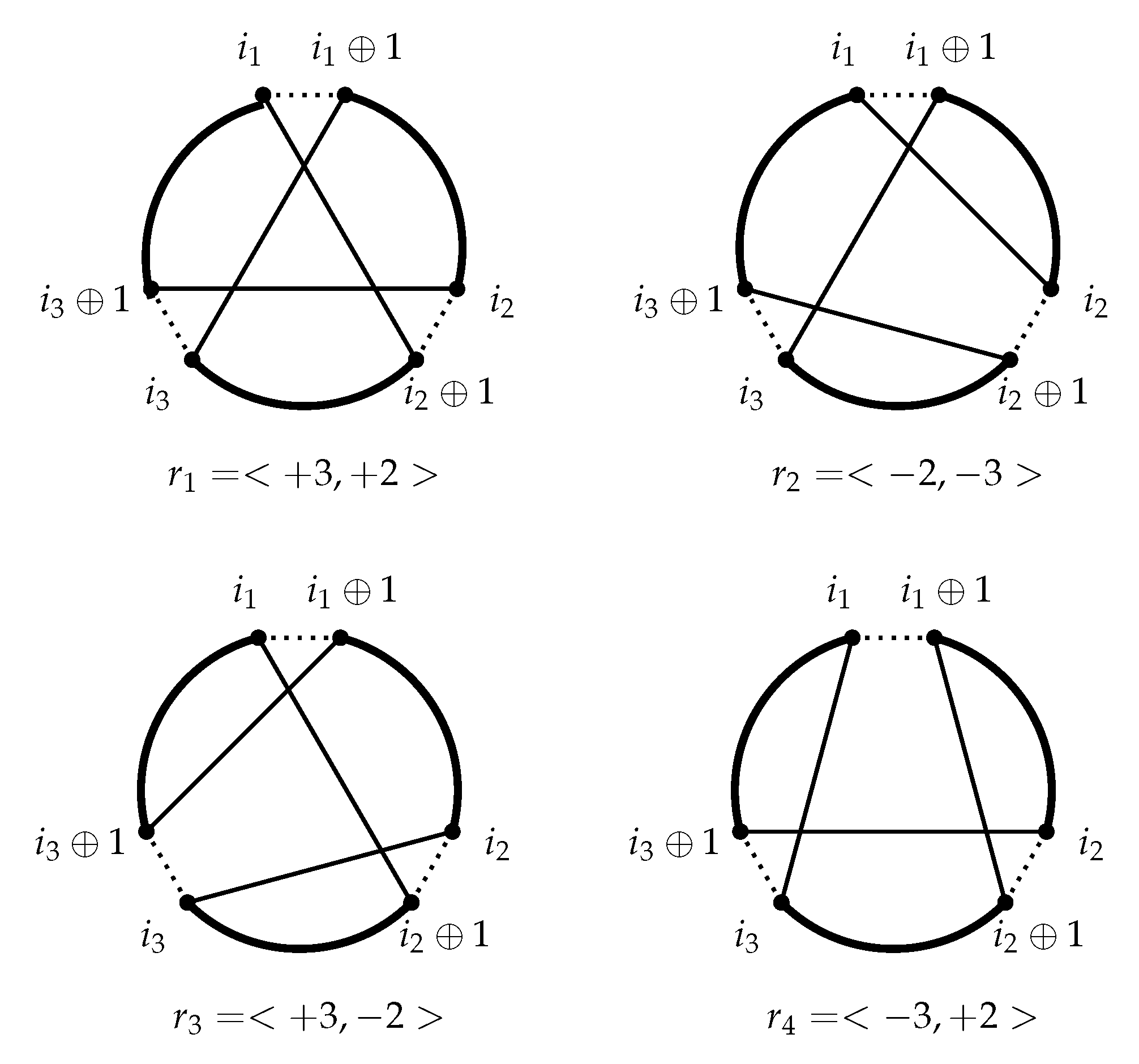
2.1. Reinsertion Schemes and Moves

Let $S=(i_1,i_2,i_3)$ be a complete selection. When the edges $R\left(S\right)$ are removed from a tour, the tour gets broken into three consecutive segments which we can label by $\{1,2,3\}$ (segment j ends at node $i_j$). Since the selection is pure, each segment is indeed a path of at least one edge. A reinsertion set patches back the segments into a new tour. If we adopt the convention to start always a tour with segment 1 traversed clockwise, the reinsertion set: (i) determines a new ordering in which the segments are visited along the tour and (ii) may cause some segments to be traversed counterclockwise. In order to represent this fact, we use a notation called a reinsertion scheme. A reinsertion scheme is a signed permutation of $\{2,3\}$. The permutation specifies the order in which the segments $2,3$ are visited after the move. The signing $-s$ tells that segment s is traversed counterclockwise, while $+s$ tells that it is traversed clockwise. For example, the third reinsertion set depicted in Figure 1 is represented by the reinsertion scheme $<+3,-2>$ since, from the end of segment 1, we jump to the beginning of segment 3 and traverse it forward. We then move to the last element of segment 2 and proceed backward to its first element. Finally, we close the tour by going back to the first element of segment 1.

There are potentially $2^2\times 2!=8$ reinsertion schemes, but for some of these the corresponding reinsertion sets are degenerate. A scheme for a pure reinsertion must not start with “$+2$”, nor end with “$+3$”, nor be $<-3,-2>$. This leaves only 4 possible schemes, let them be $r_1,\dots ,r_4$, depicted in Figure 1.

Given a selection S, the application of a reinsertion scheme r univocally determines reinsertion set $I(r,S)$ and clearly for every reinsertion set I there is an r such that $I=I(r,S)$. Therefore, a 3-OPT move if fully specified by a pair $(S,r)$ where S is a complete selection and r is a reinsertion scheme. Let us denote the set of all true 3-OPT moves by

$$\mathcal{M}=\left\{((i_1,i_2,i_3),r):(i_1,i_2,i_3)\in \mathcal{S},r\in \{r_1,r_2,r_3,r_4\}\right\}.$$

The enumeration of all moves can be done as follows: (i) we consider, in turn, each reinsertion scheme $r=r_1,\dots ,r_4$; (ii) given r, we consider all complete selections $S=(i_1,i_2,i_3)$, obtaining the moves $(S,r)$. Since step (ii) is done by complete enumeration, the cost of this procedure is $\mathsf{\Theta }\left(n^3\right)$. In the remainder of the paper we will focus on a method for lowering significantly its complexity.

2.2. The Number of True 3-OPT Moves

For generality, we state here a result which applies to K-OPT for any $K\ge 2$.

Theorem 1.

For each $K=2,\dots ,\lfloor n/2\rfloor$ the number of complete K-OPT selections is

$$\left(\genfrac{}{}{0pt}{}{n-K+1}{K}\right)-\left(\genfrac{}{}{0pt}{}{n-K-1}{K-2}\right)$$

Proof. 

Assume the indices of a selection are $0\le i_1<i_2<\dots <i_K\le \overline{n}$. Consider the tour and let: $x_1$ be the number of nodes between node 0 (included) and node $i_1$ (excluded); $x_t$, for $t=2,\dots ,K$, be the number of nodes between node $i_{t-1}$ (excluded) and node $i_t$ (excluded); $x_{K+1}$ be the number of nodes between node $i_K$ (excluded) and node $\overline{n}$ (included). Then, there are as many complete selections in a K-OPT move as the nonnegative integer solutions of the equation

$$x_1+\cdots +x_{K+1}=n-K,$$

subject to the constraints that $x_1+x_{K+1}\ge 1$, and $x_t\ge 1$ for $t=2,\dots ,K$. If we ignore the first constraint and replace $x_t$ by $y_t+1$ for $t=2,\dots ,K$ we get the equation

$$x_1+y_2+\cdots +y_K+x_{K+1}=n-2K+1,$$

in nonnegative integer variables, which, by basic combinatorics, has $\left(\genfrac{}{}{0pt}{}{(n-2K+1)+K}{K}\right)$ solutions. We then have to remove all solutions in which $x_1+x_{K+1}=0$, i.e., the solutions of the equation $y_2+\cdots +y_K=n-2K+1$, of which there are $\left(\genfrac{}{}{0pt}{}{(n-2K+1)+K-2}{K-2}\right)$. □

Corollary 1.

The number of true 3-OPT moves is

$$\frac{2n^3-18n^2+40n}{3},$$

i.e., it is, asymptotically, $\frac{2}{3}{n}^3$.

Proof. 

We know from Theorem 1 that there are $\left(\genfrac{}{}{0pt}{}{n-2}{3}\right)-(n-4)=\frac{n^3-9n^2+20n}{6}$ complete selections, and from Section 2.1 that there are 4 reinsertion schemes. By multiplying the two values we get the claim. □

In

Table 1. The number of true 2-OPT and 3-OPT moves for some n.

n	2-OPT	3-OPT
50	1175	69,000
100	4850	608,000
200	19,700	5,096,000
500	124,250	81,840,000
1000	498,500	660,680,000
2000	1,997,000	5,309,360,000
5000	12,492,500	83,183,400,000
10,000	49,985,000	666,066,800,000

we report the number of true moves for various values of n, giving a striking example of why the exploration of the 3-OPT neighborhood would be impractical unless some effective strategies were adopted.

3. Speeding-Up the Search: The Basic Idea

The goal of our work is to provide an alternative, much faster, way for finding the best move to the classical “nested-for” approach over all reinsertion schemes and indices, which is something like

• for ( $r=r_1,r_2,r_3,r_4$ )
•       for ($i_1$ = 0; $i_1\le \overline{n}-4$; $i_1$++ )
•           for ($i_2=i_1+2$; $i_2\le \overline{n}-2-\mathcal{P}(i_1=0)$; $i_2$++ )
•                for ($i_3=i_2+2$; $i_3\le \overline{n}-\mathcal{P}(i_1=0)$; $i_3$++ )
•                     evaluateMove$((i_1,i_2,i_3),r)$; [* check if move is improving. possibly update best *]

and takes time $\mathsf{\Theta }\left(n^3\right)$. (The expression $\mathcal{P}\left(A\right)$, given a predicate A returns 1 if A is true and 0 otherwise). As opposed to the brute force approach, we will call our algorithm the smart force procedure.

Our idea for speeding-up the search is based on this consideration. Suppose there is a magic box that knows all the best moves. We can inquire the box, which answers in time $O\left(1\right)$ by giving us a partial move. A partial move is the best move, but one of the selection indices has been deleted (and the partial move specifies which one). For example, we might get the answer $((4,-,9),r_2)$, and then we would know that there is some x such that the selection $(4,x,9)$, with reinsertion scheme $r_2$, is an optimal move. How many times should we inquire about the box to quickly retrieve an optimal move?

Suppose there are many optimal moves (e.g., the arc $\{0,1\}$ costs 1000 and all other arcs cost 1, so that the move $\left(\right(0,x,y),r)$ is optimal for every $(x,y)$ and r). Then we could call the box $O\left(n^2\right)$ times and get the reply $\left(\right(-,x,y),r)$ for all possible $x,y,r$ without ever getting the value of the first index of an optimal selection. However, it is clear that with just one call to the box, it is possible to compute an optimal 3-OPT move in time $O\left(n\right)$. In fact, after the box has told us the reinsertion scheme to use and the values of two indices out of three, we can enumerate the values for the missing index (i.e., expand the two indices into a triple) to determine the best completion possible.

The bulk of our work has then been to simulate, heuristically, a similar magic box, i.e., a data structure that can be queried and should return a partial move much in a similar way as described above. In our heuristic version, the box, rather than returning a partial which could certainly be completed into a best move, returns a partial move which could likely be completed into a best move. As we will see, this can already greatly reduce the number of possible candidates to be best moves. In order to assess the likelihood with which a partial move could be completed into a best solution, we will use suitable functions described in the next sections.

Since there is no guarantee that a partial move suggested by our box can be indeed completed into an optimal move, we will have to iterate over many suggestions, looking for the best one. If there are $O\left(n\right)$ iterations, given that each iteration costs us $O\left(n\right)$ we end up with an $O\left(n^2\right)$ algorithm. Some expansions will be winning, in that they produce a selection better than any one seen so far, while others will be losing, i.e., we enumerate $O\left(n\right)$ completions for the partial move but none of them beats the best move seen so far. Clearly, to have an effective algorithm we must keep the number of losing iterations small. To achieve this goal, we provide an $O\left(1\right)$ strong necessary condition that a partial move must satisfy for being a candidate to a winning iteration. When no partial move satisfies this condition, the search can be stopped since the best move found is in fact the optimal move.

The Fundamental Quantities ${\tau }^{+}$ and ${\tau }^{-}$

In this section, we define two functions of $V\times V$ into $\mathbb{R}$ fundamental for our work. Loosely speaking, these functions will be used to determine, for each pair of indices of a selection, the contribution of that pair to the value of a move. The rationale is that, the higher the contribution, the higher the probability that a particular pair is in a best selection.

The two functions are called ${\tau }^{+}\left(\right)$ and ${\tau }^{-}\left(\right)$. For each $a,b\in \{0,\dots ,\overline{n}\}$, we define ${\tau }^{+}(a,b)$ to be the difference between the cost from a to its successor and to the successor of b, and ${\tau }^{-}(a,b)$ to be the difference between the cost from a to its predecessor and to the predecessor of b:

$${\tau }^{+}(a,b)=c(a,a\oplus 1)-c(a,b\oplus 1),{\tau }^{-}(a,b)=c(a,a\ominus 1)-c(a,b\ominus 1).$$

Clearly, each of these quantities can be computed in time $O\left(1\right)$, and computing their values for a subset of possible pairs can never exceed time $O\left(n^2\right)$.

4. Searching the 3-OPT Neighborhood

As discussed in Section 2.1, the pure 3-OPT reinsertion schemes are four (see Figure 1), namely:

$$r_1=<+3,+2>r_2=<-2,-3>r_3=<+3,-2>r_4=<-3,+2>$$

(1)

Notice that $r_3$ and $r_4$ are symmetric to $r_2$. Therefore, we can just consider $r_1$ and $r_2$ since all we say about $r_2$ can be applied, mutatis mutandis (i.e., with a suitable renaming of the indices), to $r_3$ and $r_4$ as well.

Given a move $\mu =(S,r)\in \mathcal{M}$, where $S=(i_1,i_2,i_3)$, its value is the difference between the cost of the set $R\left(S\right)=\{\{i_1,i_1\oplus 1\},\{i_2,i_2\oplus 1\},\{i_3,i_3\oplus 1\}\}$ of removed edges and the cost of the reinsertion set $I(r,S)$. We will denote the value of the move μ by

$$\Delta ((i_1,i_2,i_3),r).$$

A key observation is that we can break-up the function $\Delta \left(\right)$, that has $\mathsf{\Theta }\left(n^3\right)$ possible arguments, into a sum of functions of two parameters each (each has $\mathsf{\Theta }\left(n^2\right)$ arguments). That is, we will have

$$\Delta ((i_1,i_2,i_3),r)=f_r^{12}(i_1,i_2)+f_r^{23}(i_2,i_3)+f_r^{13}(i_1,i_3),$$

(2)

for suitable functions $f_r^{12}\left(\right),f_r^{23}\left(\right),f_r^{13}\left(\right)$, each representing the contribution of a particular pair of indices to the value of the move. The domains of these functions are subsets of $\{0,\dots ,\overline{n}\}\times \{0,\dots ,\overline{n}\}$ which limit the valid input pairs to values obtained from two specific elements of a selection. For $a,b\in \{1,2,3\}$, with $a<b$, let us define

$${\mathcal{S}}_{ab}:=\{(x,y):\exists (v_1,v_2,v_3)\in \mathcal{S}\mathrm{with}{v}_a=x\mathrm{and}{v}_b=y\}.$$

(3)

Then the domain of $f_r^{12}$ is ${\mathcal{S}}_{12}$, the domain of $f_r^{23}$ is ${\mathcal{S}}_{23}$ and the domain of $f_r^{13}$ is ${\mathcal{S}}_{13}$.

The functions $f_r^{12},f_r^{23},f_r^{13}$ can be obtained through the functions ${\tau }^{+}\left(\right)$ and ${\tau }^{-}\left(\right)$ as follows:

[r₁: ]

We have $I\left(r_1\right)=\{\{i_1,i_2\oplus 1\},\{i_2,i_3\oplus 1\},\{i_1\oplus 1,i_3\}\}$ (see Figure 1) so that $\Delta ((i_1,i_2,i_3),r_1)=$

$$\begin{array}{cc}\hfill & =\left[c(i_1,i_1\oplus 1)+c(i_2,i_2\oplus 1)+c(i_3,i_3\oplus 1)\right]-\left[c(i_1,i_2\oplus 1)+c(i_2,i_3\oplus 1)+c(i_1\oplus 1,i_3)\right]\hfill \\ \hfill & =\left[c(i_1,i_1\oplus 1)-c(i_1,i_2\oplus 1)\right]+\left[c(i_2,i_2\oplus 1)-c(i_2,i_3\oplus 1)\right]+\left[c(i_3,i_3\oplus 1)-c(i_3,i_1\oplus 1)\right]\hfill \\ \hfill & ={\tau }^{+}(i_1,i_2)+{\tau }^{+}(i_2,i_3)+{\tau }^{+}(i_3,i_1).\hfill \end{array}$$

(4)

The three functions are

$f_{r_1}^{12}:(x,y)\in {\mathcal{S}}_{12}\mapsto {\tau }^{+}(x,y)$;

$f_{r_1}^{23}:(x,y)\in {\mathcal{S}}_{23}\mapsto {\tau }^{+}(x,y)$;

$f_{r_1}^{13}:(x,y)\in {\mathcal{S}}_{13}\mapsto {\tau }^{+}(y,x)$.

[r₂: ]

We have $I\left(r_2\right)=\{\{i_1,i_2\},\{i_2\oplus 1,i_3\oplus 1\},\{i_1\oplus 1,i_3\}\}$ (see Figure 1) so that $\Delta ((i_1,i_2,i_3),r_2)=$

$$\begin{array}{cc}\hfill & =\left[c(i_1,i_1\oplus 1)+c(i_2,i_2\oplus 1)+c(i_3,i_3\oplus 1)\right]-\left[c(i_1,i_2)+c(i_2\oplus 1,i_3\oplus 1)+c(i_1\oplus 1,i_3)\right]\hfill \\ \hfill & =\left[c(i_1,i_1\oplus 1)-c(i_1,i_2)\right]+\left[c(i_2\oplus 1,i_2)-c(i_2\oplus 1,i_3\oplus 1)\right]+\left[c(i_3,i_3\oplus 1)-c(i_3,i_1\oplus 1)\right]\hfill \\ \hfill & ={\tau }^{+}(i_1,i_2\ominus 1)+{\tau }^{-}(i_2\oplus 1,i_3\oplus 2)+{\tau }^{+}(i_3,i_1).\hfill \end{array}$$

(5)

The three functions are

$f_{r_2}^{12}:(x,y)\in {\mathcal{S}}_{12}\mapsto {\tau }^{+}(x,y\ominus 1)$;

$f_{r_2}^{23}:(x,y)\in {\mathcal{S}}_{23}\mapsto {\tau }^{-}(x\oplus 1,y\oplus 2)$;

$f_{r_2}^{13}:(x,y)\in {\mathcal{S}}_{13}\mapsto {\tau }^{+}(y,x)$.

(For convenience, these functions, as well as the functions of some other moves described later on, are also reported in

Table 2. Expressing $\Delta ((i_1,i_2,i_3),r)$ as a sum $f_r^{12}(i_1,i_2)+f_r^{23}(i_2,i_3)+f_r^{13}(i_1,i_3)$.

r	$f_r^{12}(x,y)$	$f_r^{23}(x,y)$	$f_r^{13}(x,y)$
$r_1$	${\tau }^{+}(x,y)$	${\tau }^{+}(x,y)$	${\tau }^{+}(y,x)$
$r_2$	${\tau }^{+}(x,y\ominus 1)$	${\tau }^{-}(x\oplus 1,y\oplus 2)$	${\tau }^{+}(y,x)$
$r_3$	${\tau }^{+}(x,y)$	${\tau }^{+}(x,y\ominus 1)$	${\tau }^{-}(y\oplus 1,x\oplus 2)$
$r_4$	${\tau }^{-}(x\oplus 1,y\oplus 2)$	${\tau }^{+}(x,y)$	${\tau }^{+}(y,x\ominus 1)$
$r_5$	${\tau }^{+}(y,x)+{\tau }^{-}(y,x)$	${\tau }^{+}(y,x)+{\tau }^{-}(y,x)$	${\tau }^{+}(x,y)+{\tau }^{-}(x,y)$
$r_6$	${\tau }^{+}(x,y)+{\tau }^{-}(x,y)$	${\tau }^{+}(x,y)+{\tau }^{-}(x,y)$	${\tau }^{+}(y,x)+{\tau }^{-}(y,x)$
$r_7$	${\tau }^{+}(x,y)+{\tau }^{+}(y,x)$	${\tau }^{-}(x,y)+{\tau }^{-}(y,x)$	${\tau }^{+}(x\ominus 1,y\ominus 1)+{\tau }^{-}(y\oplus 1,x\oplus 1)$
$r_8$	${\tau }^{-}(x\oplus 1,y\oplus 2)+{\tau }^{-}(y,x\oplus 1)$	${\tau }^{+}(x,y)+{\tau }^{-}(y,x)$	${\tau }^{+}(x\ominus 1,y\ominus 2)+{\tau }^{+}(y,x\ominus 1)$
$r_9$	${\tau }^{-}(x\oplus 1,y\oplus 1)+{\tau }^{+}(x\ominus 1,y\ominus 1)+{\tau }^{+}(y\ominus 1,x\ominus 1)$	${\tau }^{-}(x\oplus 1,y\oplus 2)$	${\tau }^{+}(y,x\ominus 1)$

of Section 6). The functions $f_r^{12},f_r^{23},f_r^{13}$ are used in our procedure in two important ways. First, we use them to decide which are the most likely pairs of indices to belong in an optimal selection for r (the rationale being that, the higher a value $f_r(x,y)$, the more likely it is that $(x,y)$ belongs in a good selection).

Secondly, we use them to discard from consideration some moves which cannot be optimal. These are the moves such that no two of the indices give a sufficiently large contribution to the total. Better said, we keep in consideration only moves for which at least one contribution of two indices is large enough. With respect to the strategy outlined in Section 3, this corresponds to a criterion for deciding if a partial move suggested by our heuristic box is worth expanding into all its completions.

Assume we want to find the best move overall and the best move we have seen so far (the current “champion”) is ${\mu }^{*}$. We make the key observation that for a move $((i_1,i_2,i_3),r)$ to beat ${\mu }^{*}$ it must be

$$\left(f_r^{12}(i_1,i_2)>\frac{\Delta \left({\mu }^{*}\right)}{3}\right)\vee \left(f_r^{23}(i_2,i_3)>\frac{\Delta \left({\mu }^{*}\right)}{3}\right)\vee \left(f_r^{13}(i_1,i_3)>\frac{\Delta \left({\mu }^{*}\right)}{3}\right).$$

These three conditions are not exclusive but possibly overlapping, and in our algorithm, we will enumerate only moves that satisfy at least one of them. Furthermore, we will not enumerate these moves with a complete enumeration, but rather from the most promising to the least promising, stopping as soon as we realize that no move has still the possibility of being the best overall.

The most appropriate data structure for performing this kind of search (which hence be used for our heuristic implementation of the magic box described in Section 3) is the Max-Heap. A heap is perfect for taking the highest-valued elements from a set, in decreasing order. It can be built in linear time with respect to the number of its elements and has the property that the largest element can be extracted in logarithmic time, while still leaving a heap.

We then build a max-heap H whose elements are records of type

$$[x,y,f,\alpha ,r],$$

where $\alpha \in \{12,13,23\}$, $r\in \{r_1,r_2,r_3,r_4\}$, $(x,y)\in {\mathcal{S}}_{\alpha }$, and $f:=f_r^{\alpha }(x,y)$. The heap elements correspond to partial moves. The heap is organized according to the values of f, and the field $\alpha$ is a label identifying which selection indices are associated to a given heap entry. We initialize H by putting in it an element for each $(x,y)$, r and $\alpha$ such that $f_r^{\alpha }(x,y)>\Delta \left({\mu }^{*}\right)/3$. We then start to extract the elements from the heap. Let us denote by $[x^j,y^j,f^j,{\alpha }^j,r^j]$ the j-th element extracted. Heuristically, we might say that $x^1$ and $y^1$ are the most likely values that a given pair of indices (specified by ${\alpha }^1$) can take in the selection of a best-improving move, since these values give the largest possible contribution to the move value (2). We will keep extracting the maximum $[x^j,y^j,f^j,{\alpha }^j,r^j]$ from the heap as long as $f^j>\Delta \left({\mu }^{*}\right)/3$. This does not mean that we will extract all the elements of H, since $\Delta \left({\mu }^{*}\right)$ could change (namely, increase) during the search and hence the extractions might terminate before the heap is empty.

Each time we extract the heap maximum, we have that $x^j$ and $y^j$ are two possible indices out of three for a candidate move to beat ${\mu }^{*}$. With a linear-time scan, we then enumerate the third missing index (identified by ${\alpha }^j$) and see if we get indeed a better move than ${\mu }^{*}$. For example, if ${\alpha }^j=13$ then the missing index is $i_2$ and we run a for-loop over $i_2$, with $x^j+2\le i_2\le y^j-2$, checking each time if the move $((x^j,i_2,y^j),r^j)$ is a better move than ${\mu }^{*}$. Whenever this is the case, we update ${\mu }^{*}$. Note that, since $\Delta \left({\mu }^{*}\right)$ increases, the number of elements still in the heap for which $f>\Delta \left({\mu }^{*}\right)/3$ after updating the champion may be considerably smaller than it was before the update.

Lemma 1.

When the procedure outlined above terminates, ${\mu }^{*}$ is an optimal move.

Proof. 

Suppose, by contradiction, that there exists a move $\mu =((w_1,w_2,w_3),r)$ better than ${\mu }^{*}$. Since $\Delta ((w_1,w_2,w_3),r)>\Delta \left({\mu }^{*}\right)$, there exists at least one pair $a<b\in \{1,2,3\}$ such that $f_r^{ab}(w_a,w_b)>\Delta \left({\mu }^{*}\right)/3$. Then the partial move $(w_a,w_b,f_r^{ab}(w_a,w_b),ab,r)$ would have eventually been popped from the heap and evaluated, producing a move better than ${\mu }^{*}$. Therefore the procedure could not have ended with the move ${\mu }^{*}$. □

Assume L denotes the initial size of the heap and M denotes the number of elements that are extracted from the heap overall. Then the cost of the procedure is $O(n^2+L+M(logL+n))$ since: (i) $\mathsf{\Theta }\left(n^2\right)$ is the cost for computing the $\tau$ values; (ii) $\mathsf{\Theta }\left(L\right)$ is the cost for building the heap; (iii) for each of the M elements extracted from the heap we must pay $O(logL)$ for re-adjusting the heap, and then we complete the move in $O\left(n\right)$ ways. 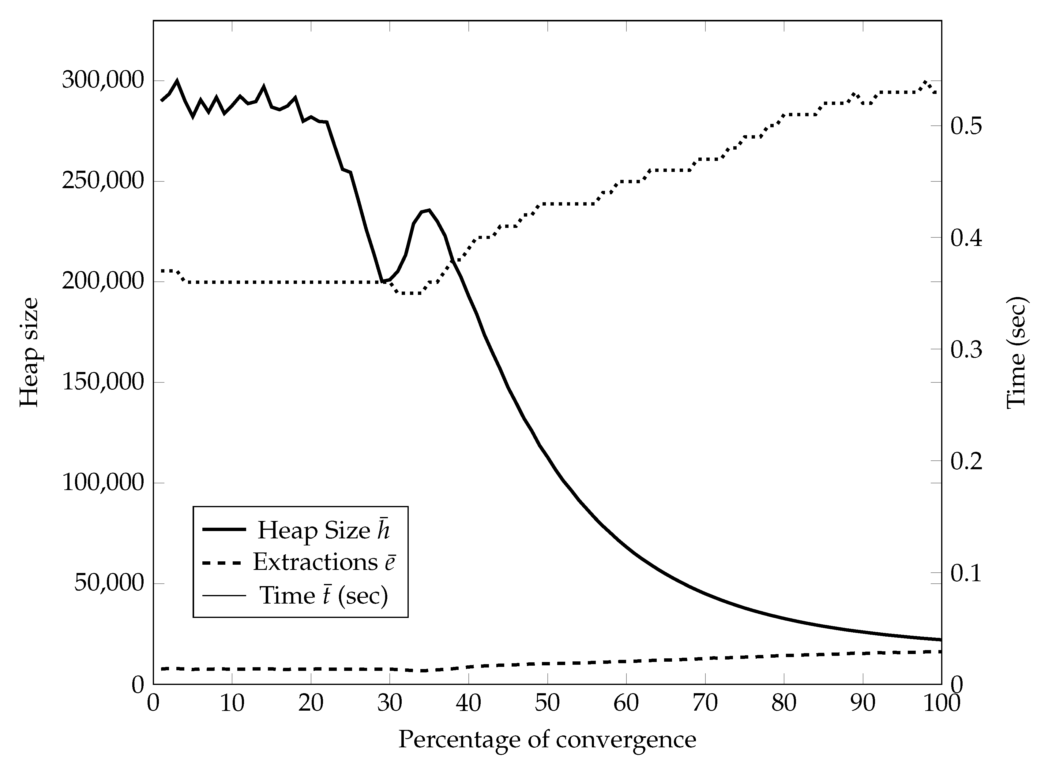Worst-case, the procedure has complexity $O\left(n^3\right)$ like complete enumeration but, as we will show in our computational experiments, it is much smaller in practice. In fact, on our tests the complexity was growing slightly faster than a quadratic function of n (see Section 5). This is because the $Mn$ selections which are indeed evaluated for possibly becoming the best move have a much bigger probability of being good than a generic selection, since two of the three indices are guaranteed to help the value of the move considerably.

4.1. Worst-Case Analysis

A theoretical result stated in [11] shows that no algorithm with a less than cubic worst-case complexity is possible for 3-OPT (under the widely believed ALL-PAIRS SHORTEST PAIR conjecture). In light of this result, we expected that there should exist some instances which force our algorithm to require cubic time. In particular, we have found the following example.

Theorem 2.

The Smart Force algorithm has a worst-case complexity $\mathsf{\Theta }\left(n^3\right)$.

Proof. 

Clearly, the complexity is $O\left(n^3\right)$ since there are $O\left(n^2\right)$ partial moves and the evaluation of each of them takes $O\left(n\right)$ time. To show the lower bound $\mathsf{\Omega }\left(n^3\right)$ consider the following instance.

Fix any $ϵ>0$ and, for each $0\le i<j\le \overline{n}$, define $c(i,j)$ to be

$$c(i,j)=\left\{\begin{array}{cc}1+4ϵ\hfill & \mathrm{if}i=j\left(\mathrm{mod}2\right)\hfill \\ 1\hfill & \mathrm{if}i\ne j\left(\mathrm{mod}2\right)\mathrm{and}|i-j|>1\hfill \\ 1+ϵ\hfill & \mathrm{if}|i-j|=1\hfill \end{array}\right.$$

(Notice that if $ϵ\le 2/3$ this instance is in fact metric). For these costs, the current tour $(0,\dots ,\overline{n})$ is a local optimum. In fact, for each selection, $(i_1,i_2,i_3)$ at least two of the nodes have the same parity and hence at least one edge of value $1+4ϵ$ would be introduced by a move. Therefore the inserted edges would have cost at least $3+4ϵ$, while the removed edges have cost $3+3ϵ$.

We have

$${\tau }^{+}(i,j)=c(i,i+1)-c(i,j+1)=\left\{\begin{array}{cc}1+ϵ-1=ϵ\hfill & \mathrm{if}i=j\left(\mathrm{mod}2\right)\hfill \\ 1+ϵ-1-4ϵ=-3ϵ\hfill & \mathrm{if}i\ne j\left(\mathrm{mod}2\right)\hfill \end{array}\right.$$

Therefore, for each of the $\mathsf{\Theta }\left(n^2\right)$ pairs $(i,j)$ such that i and j have the same parity, it is ${\tau }^{+}(i,j)=ϵ>0$. Since

$$\Delta ((i_1,i_2,i_3),r_1)={\tau }^{+}(i_1,i_2)+{\tau }^{+}(i_2,i_3)+{\tau }^{+}(i_3,i_1),$$

each such pair would be put in the heap and evaluated, fruitlessly, for a total running time of $\mathsf{\Omega }\left(n^3\right)$. □

4.2. Implementing the Search Procedure

We now describe more formally the procedure that finds the best improving 3-OPT move. To simplify the description of the code, we will make use of a global variable ${\mu }^{*}$ representing the current champion move. Initially ${\mu }^{*}$ is NULL, and we extend the function $\Delta \left(\right)$ by defining $\Delta \left(\mathtt{NULL}\right):=0$.

The main procedure is Find3-OPTmove (Procedures 1 and 2). The procedure starts by setting ${\mu }^{*}$ to a solution for which, possibly, $\Delta \left({\mu }^{*}\right)>0$. This is not strictly necessary, and setting ${\mu }^{*}$ to NULL would work too, but a little effort in finding a “good” starting champion can yield a smaller heap and thus a faster, overall, procedure. In our case, we have chosen to just sample $4n$ random solutions and keep the best.

Procedure 1 Find3-OPTmove

1. ${\mu }^{*}\leftarrow \mathtt{startingSolution}\left(\right)$

2. $H\leftarrow \mathtt{buildHeap}\left(\right)$

3. while $\left(H\left[1\right].\mathtt{val}>\Delta \left({\mu }^{*}\right)/3\right)$

4.   $(x,y,\alpha ,r)\leftarrow \mathtt{extractMax}\left(H\right)$

5.   for $z\in \mathtt{range}\mathtt{3}\mathtt{rd}(x,y,\alpha )$

6.       $(i,j,k)\leftarrow \mathtt{selection}(x,y,z,\alpha )$

7.       if$(\Delta ((i,j,k),r)>\Delta \left({\mu }^{*}\right))$ then  /* update global optimum */

8.       ${\mu }^{*}\leftarrow$ ((i, j, k), r)

9. /* if ${\mu }^{*}$ = NULL there are no improving moves */

Procedure 2StartingSolution ()

Output: move $\mu$ (such that $\Delta \left(\mu \right)\ge 0$)

1. $\mu \leftarrow \mathtt{NULL}$

2. for $r=r_1,r_2,r_3,r_4$

3.    for $t=1$ to n

4.    $(i,j,k)\leftarrow \mathtt{randomSelection}\left(\right)$

5.    if $(\Delta ((i,j,k),r)>\Delta (\mu \left)\right)$ then

6.      $\mu \leftarrow \left(\right(i,j,k),r)$

7. return $\mu$

The procedure then builds a max-heap (see Procedure 3 BuildHeap) containing an entry for each $r\in r_1,\dots ,r_4$, $\alpha \in \{12,23,13\}$ and $(x,y)\in {\mathcal{S}}_{\alpha }$ such that $f_r^{\alpha }(x,y)>\Delta \left({\mu }^{*}\right)/3$. The specific functions $f_r^{\alpha }$, for each $\alpha$ and r, are detailed in Table 2 of Section 6. The heap is implemented by an array H of records with five fields: $\mathtt{x}$ and $\mathtt{y}$, which represent two indices of a selection; $\mathtt{alpha}$ which is a label identifying the two type of indices; $\mathtt{val}$ which is the numerical value used as the key to sort the heap; and $\mathtt{scheme}$ which is a label identifying a reinsertion scheme. By using the standard implementation of a heap (see, e.g., [15]), the array corresponds to a complete binary tree whose nodes are stored in consecutive entries from 1 to $H.\mathtt{SIZE}$. The left son of node $H\left[t\right]$ is $H\left[2t\right]$, while the right son is $H[2t+1]$. The father of node $H\left[t\right]$ is $H[t.\mathrm{div}.2]$. The heap is such that the key of each node $H\left[t\right]$ is the largest among all the keys of the subtree rooted at $H\left[t\right]$.

In the procedure BuildHeap we use a function $\mathtt{range}\mathtt{1}\mathtt{st}\mathtt{2}\mathtt{nd}\left(\alpha \right)$ which returns the set of all values that a pair $(x,y)$ of indices of type $\alpha$ can assume. More specifically,

-

$\mathtt{range}\mathtt{1}\mathtt{st}\mathtt{2}\mathtt{nd}\left(12\right):=\{(x,y):0\le x<x+2\le y\le \overline{n}-2-\mathcal{P}(x=0)\}$ /* x is $i_1$ and y is $i_2$ */

-

$\mathtt{range}\mathtt{1}\mathtt{st}\mathtt{2}\mathtt{nd}\left(23\right):=\{(x,y):2+\mathcal{P}(y=\overline{n})\le x<x+2\le y\le \overline{n}\}$ /* x is $i_2$ and y is $i_3$ */

-

$\mathtt{range}\mathtt{1}\mathtt{st}\mathtt{2}\mathtt{nd}\left(13\right):=\{(x,y):0\le x<x+4\le y\le \overline{n}-\mathcal{P}(x=0)\}$ /* x is $i_1$ and y is $i_3$ */

Procedure 3BuildHeap ()

Output: heap H

1.  new H

2.  $c\leftarrow 0$

3.  for $r=r_1,r_2,r_3,r_4$

4.        for $\alpha =12,23,13$

5.            for $(x,y)\in \mathtt{range}\mathtt{1}\mathtt{st}\mathtt{2}\mathtt{nd}\left(\alpha \right)$

6.                  if $\left(f_r^{\alpha }(x,y)>\Delta \left({\mu }^{*}\right)/3\right)$ then

7.                     $c\leftarrow c+1$

8.                     $H\left[c\right].\mathtt{x}\leftarrow x$

9.                     $H\left[c\right].\mathtt{y}\leftarrow y$

10.                      $H\left[c\right].\mathtt{val}\leftarrow f_r^{\alpha }(x,y)$

11.                      $H\left[c\right].\mathtt{alpha}\leftarrow \alpha$

12.                      $H\left[c\right].\mathtt{scheme}\leftarrow r$

13.  $H.\mathtt{SIZE}\leftarrow c$

14.  for $t\leftarrow \lfloor \frac{H.\mathtt{SIZE}}{2}\rfloor ,\dots ,2,1$

15.        $\mathtt{heapify}(H,t)$    /* turns the array into a heap */

16.  return H

BuildHeap terminates with a set of calls to the procedure Heapify (a standard procedure for implementing heaps), described in Procedure 4. To simplify the code, we assume $H\left[t\right].\mathtt{val}$ to be defined also for $t>H.\mathtt{SIZE}$, with value $-\infty$. The procedure Heapify$(H,t)$ requires that the subtree rooted at t respects the heap structure at all nodes, except, perhaps, at the root. The procedure then adjusts the keys so that the subtree rooted at t becomes indeed a heap. The cost of heapify is linear in the height of the subtree. The loop of line 14 in procedure BuildHeap turns the unsorted array H into a heap, working its way bottom-up, in time $O(H.\mathtt{SIZE})$.

Procedure 4Heapify$(H,t)$

Input: array H, integer $t\in \{1,\dots H.\mathtt{SIZE}\}$

1.  $ls\leftarrow 2t$  /* left son */

2.  $rs\leftarrow 2t + 1$  /* right son */

3.  if ($H\left[ls\right].\mathtt{val} > H\left[t\right].\mathtt{val}$) then large ← ls else large ← t

4.  if ($H\left[rs\right].\mathtt{val} > H\left[large\right].\mathtt{val}$) then large ← rs

5.  if (large ≠ t) then

6.       $H\left[t\right]\leftrightarrow H\left[large\right]$   /* swaps $H\left[t\right]$ with the largest of its sons */

7.       $\mathtt{heapify}(H,large)$

Coming back to Find3-OPTMove, once the heap has been built, a loop (lines 3–8) extracts the partial moves from the heap, from the most to the least promising, according to their value (field val). For each partial move popped from the heap we use a function $\mathtt{range}\mathtt{3}\mathtt{rd}(x,y,\alpha )$ to obtain the set of all values for the missing index with respect to a pair $(x,y)$ of type $\alpha$. More specifically.

-

$\mathtt{range}\mathtt{3}\mathtt{rd}(x,y,12):=\{z:y+2\le z\le \overline{n}-\mathcal{P}(x=0)\}$ /* missing index is $i_3$ */

-

$\mathtt{range}\mathtt{3}\mathtt{rd}(x,y,23):=\{z:0+\mathcal{P}(y=\overline{n})\le z\le x-2\}$ /* missing index is $i_1$ */

-

$\mathtt{range}\mathtt{3}\mathtt{rd}(x,y,13):=\{z:x+2\le z\le y-2\}$ /* missing index is $i_2$ */.

We then complete the partial move in all possible ways, and each way is compared to the champion to see if there has been an improvement (line 7). Whenever the champion changes, the condition for loop termination becomes easier to satisfy than before.

In line 6 we use a function $\mathtt{selection}(x,y,z,\alpha )$ that, given three indices x, y, z and a pair type $\alpha$, rearranges the indices so as to return a correct selection. In particular, $\mathtt{selection}(x,y,z,12):=(x,y,z)$, $\mathtt{selection}(x,y,z,23):=(z,x,y)$, and $\mathtt{selection}(x,y,z,13):=(x,z,y)$.

The procedure ExtractMax (in the Procedure 5) returns the element of a maximum value of the heap (which must be in the root node, i.e., $H\left[1\right]$). It then replaces the root with the leaf $H[H.\mathtt{SIZE}]$ and, by calling $\mathtt{heapify}(H,1)$, it moves it down along the tree until the heap property is again fulfilled. The cost of this procedure is $O(log(H.\mathtt{SIZE}\left)\right)$.

Procedure 5ExtractMax$\left(H\right)$

Input: heap H

Output: the partial move $(x,y,\alpha ,r)$ of maximum value in H

1.  $(x,y,\alpha ,r)\leftarrow \left(H\right[1].\mathtt{x},H[1].\mathtt{y},H[1].\mathtt{alpha},H[1].\mathtt{scheme})$ /* gets the max element */

2.  $H\left[1\right]\leftarrow H[H.\mathtt{SIZE}]$ /* overwrites it */

3.  $H.\mathtt{SIZE}\leftarrow H.\mathtt{SIZE}-1$

4.  $\mathtt{heapify}(H,1)$ /* restores the heap */

5.  return $(x,y,\alpha ,r)$

5. Computational Results

In this section, we report on our extensive computational experiments showing the effectiveness of the approach we propose. All tests were run on a Intel^®Core^TM i7-7700 8CPU under Linux Ubuntu, equipped with 16 GB RAM at 3.6GHz clock. The programs were implemented in C, compiled under gcc 5.4.0 and are available upon request,

5.1. Instance Types

The experiments were run on two types of graphs: (i) random graphs generated by us and (ii) instances from the standard benchmark repository TSPLIB [16]. The random graphs are divided into three categories:

-

Uniform (UNI): complete graphs in which the edge costs are independent random variables drawn uniformly in the range $[0,1]$.

-

Gaussian (GAU): complete graphs in which the edge costs are independent random variables drawn according to the Gaussian distribution $N(\mu ,\sigma )$ with mean $\mu =0.5$ and standard deviation $\sigma =0.1$.

-

Geometric (GEO): complete graphs in which the edge costs are the Euclidean distances between n random points of the plane. In particular, the points are generated within a circle of radius 1 by drawing, u.a.r. a pair of polar coordinates $(d,\alpha )$, where $d\in [0,1]$ and $\alpha \in [0,2\pi ]$.

Our goal in using more than one type of random distribution was to assess if our method is sensible, and if so, to what extent, to variation in the type of edge costs involved. The results will show that the GEO instances are slightly harder to tackle, while UNI and GAU are more or less equivalent.

5.2. Experiment 1: Best Move from a Random Tour

5.2.1. Random Instances

In a first set of experiments we compared our method to the brute force (BF) approach on random instances of the type described before. In particular, for each type of random graph we generated instances of sizes $n_1,\dots ,n_9$ where we set $n_1=400$ and $n_{i+1}=\lceil \sqrt{2}\times n_i\rceil$ for $i=1,\dots ,8$. This geometric increase is chosen so that we should see a doubling of the running times in going from $n_i$ to $n_{i+1}$ with a quadratic method, while the ratio should be about $2\sqrt{2}\simeq 2.83$ with the cubic BF approach.

For each given size $n_i$ we generated 1000 random instances. Finally, for each random instance, we generated a random initial tour and found the best 3-OPT move with both smart force (SF) and BF.

In

Table 3. Comparing smart force (SF) and brute force (BF) in finding one Best Improving move starting from a random tour and using pure 3-OPT moves only (averaged over 1000 attempts).

Type	Size	Time (S)			Number of Evaluated Triples			Ratio Against the Previous Size
		BF_avg	SF_avg	Speed-up	BF	SF_avg	Reduction	SF_time	SF_eval	BF_time	BF_eval
UNI	400	0.65	0.01	75×	41,712,000	177,247	235×
	566	1.80	0.01	136×	118,966,408	352,174	337×	1.53	1.98	2.79	2.85
	800	5.08	0.03	187×	337,504,000	689,730	489×	2.05	1.95	2.81	2.83
	1131	14.37	0.09	160×	956,827,508	1,378,905	693×	3.31	1.99	2.82	2.83
	1600	40.75	0.26	157×	2,715,328,000	2,709,608	1002×	2.89	1.96	2.83	2.83
	2262	115.30	0.64	179×	7,685,229,448	5,406,134	1421×	2.47	1.99	2.82	2.83
	3200	326.78	1.60	204×	21,783,936,000	10,616,608	2051×	2.48	1.96	2.83	2.83
	4524	924.09	3.43	269×	61,604,454,080	21,248,234	2899×	2.14	2.00	2.82	2.82
	6400	2617.77	7.33	356×	174,516,992,000	42,114,426	4143×	2.13	1.98	2.83	2.83
	Avg							2.37	1.97	2.81	2.83
GAU	400	0.65	0.01	85×	41,712,000	115,939	359×
	566	1.79	0.01	156×	118,966,408	226,615	524×	1.50	1.95	2.73	2.85
	800	5.13	0.02	221×	337,504,000	426,427	791×	2.02	1.88	2.87	2.83
	1131	14.23	0.07	191×	956,827,508	838,088	1141×	3.19	1.96	2.77	2.83
	1600	41.16	0.23	181×	2,715,328,000	1,616,552	1679×	3.04	1.92	2.89	2.83
	2262	114.15	0.50	227×	7,685,229,448	3,195,748	2404×	2.21	1.97	2.77	2.83
	3200	330.05	1.17	282×	21,783,936,000	6,196,979	3515×	2.33	1.93	2.89	2.83
	4524	914.85	2.37	386×	61,604,454,080	12,463,367	4942×	2.02	2.01	2.77	2.82
	6400	2643.95	5.20	508×	174,516,992,000	23,596,890	7395×	2.19	1.89	2.89	2.83
	Avg							2.31	1.93	2.82	2.83
GEO	400	0.64	0.01	73×	41,712,000	195,280	213×
	566	1.82	0.01	133×	118,966,408	415,980	285×	1.57	2.13	2.85	2.85
	800	5.03	0.03	143×	337,504,000	904,099	373×	2.55	2.17	2.76	2.83
	1131	14.52	0.10	143×	956,827,508	1,922,566	497×	2.90	2.12	2.88	2.83
	1600	40.34	0.30	133×	2,715,328,000	4,159,708	652×	2.98	2.16	2.77	2.83
	2262	116.45	0.79	146×	7,685,229,448	9,338,712	822×	2.62	2.24	2.88	2.83
	3200	323.51	2.03	159×	21,783,936,000	21,611,397	1007×	2.56	2.31	2.77	2.83
	4524	933.33	4.45	209×	61,604,454,080	48,245,203	1276×	2.19	2.23	2.88	2.82
	6400	2591.60	10.84	239×	174,516,992,000	112,442,210	1552×	2.43	2.33	2.77	2.83
	Avg							2.47	2.21	2.82	2.83

we report the results of the experiment. The table is divided vertically into three parts. The first part reports the average running time of the two approaches (columns ${\mathrm{BF}}_{\mathrm{avg}}$ and ${\mathrm{SF}}_{\mathrm{avg}}$) and the speed-up achieved by smart force over brute force. We can see that in our instances smart force is at least 70 times faster and as much as 500 times faster than brute force. Similar results are reported in the second vertical part, in which we focus on the number of triples evaluated by the two methods. Clearly, the average for the BF method is indeed a constant, since all triples must be evaluated. SF, on the other hand, evaluates a much smaller number of triples, going from a minimum of 200 times less up to 7000 times less triples than BF. Notice how the saving in the running time is actually smaller than the saving in the number of triples evaluated. This is due to the overhead needed for building and updating the heap. The standard deviations for the SF times (not reported in the table for space reasons) were in the range 10–25% of the mean value, while for the number of evaluated triples the standard deviations were between 30% and 40%.

In the final vertical section, we focus on the empirical estimate of a complexity function for the running time and the number of evaluated triples of the smart force approach. In particular, the column ${\mathrm{SF}}_{\mathrm{time}}$ reports the ratio between the average time of SF on instances of size $n_k$ and $n_{k-1}$. Given the way that we defined the $n_k$’s, a value $\simeq 2$ on this column would be indicative of a quadratic algorithm, while a value $\simeq 2\sqrt{2}\simeq 2.83$ would be indicative of a cubic algorithm.

The average ratios for the running time of the SF algorithm were 2.37, 2.31 and 2.47 for the UNI, GAU and GEO instances respectively. These values are indicative of an algorithm whose empirical average complexity is definitely sub-cubic, but not quite quadratic. A reasonably good fit with an experimental upper bound to the time complexity is $O\left(n^{2.5}\right)$ (see Figure 2).

The column labeled ${\mathrm{SF}}_{\mathrm{eval}}$ reports the same type of ratios but this time relatively to the number of triples evaluated by SF. We can see that for UNI and GAU graphs the number of triples grows almost exactly as a quadratic function of n. Notice that evaluating less than a quadratic number of triples would be impossible, since each edge must be looked at, and there is a quadratic number of edges. Again, the class of graphs GEO seems to be slightly harder than UNI and GAU.

For completeness, in columns ${\mathrm{BF}}_{\mathrm{time}}$ and ${\mathrm{BF}}_{\mathrm{eval}}$ we report the same type of values for the BF method.

The main message from the table is that while finding the best 3-OPT move for a tour of about 6000 nodes with the classical BF approach can take more than half an hour, with our approach it can be done in 5 s or so.

5.2.2. TSPLIB Instances

We have then run the same type of experiment on instances from the TSPLIB. For each instance, we generated 1000 random starting tours and found the best 3-OPT move. The results are reported in

Table 4. Comparing SF and BF in finding one Best Improving move on Traveling Salesman Problem Library (TSPLIB) instances starting from a random tour (averaged over 1000 attempts).

Type	Name	Size	Time (S)			Number of Evaluated Triples
			BF_avg	SF_avg	Speed-up	BF	SF_avg	Reduction
euc2d	kroA100	100	0.01	0.01	1×	608,000	33,124	18×
euc2d	kroB100	100	0.01	0.01	1×	608,000	34,449	17×
euc2d	kroC100	100	0.01	0.01	1×	608,000	36,688	16×
euc2d	kroD100	100	0.01	0.01	1×	608,000	28,025	21×
euc2d	kroE100	100	0.01	0.01	1×	608,000	39,838	15×
euc2d	rd100	100	0.01	0.01	1×	608,000	20,005	30×
euc2d	eil101	101	0.01	0.01	1×	627,008	20,652	30×
euc2d	lin105	105	0.01	0.01	1×	707,000	38,662	18×
euc2d	pr107	107	0.01	0.01	1×	749,428	99,522	7×
explicit	gr120	120	0.02	0.01	2×	1,067,200	52,980	20×
euc2d	pr124	124	0.02	0.01	2×	1,180,480	46,661	25×
euc2d	bier127	127	0.02	0.01	2×	1,270,508	57,122	22×
euc2d	ch130	130	0.02	0.01	2×	1,365,000	31,174	43×
euc2d	pr136	136	0.02	0.01	2×	1,567,808	58,883	26×
geo	gr137	137	0.02	0.01	2×	1,603,448	86,440	18×
euc2d	pr144	144	0.02	0.01	2×	1,868,160	51,295	36×
euc2d	ch150	150	0.02	0.01	2×	2,117,000	47,146	44×
euc2d	kroA150	150	0.02	0.01	2×	2,117,000	93,533	22×
euc2d	kroB150	150	0.02	0.01	2×	2,117,000	120,822	17×
euc2d	pr152	152	0.02	0.01	2×	2,204,608	63,987	34×
euc2d	u159	159	0.03	0.01	3×	2,530,220	127,254	19×
explicit	si175	175	0.03	0.01	3×	3,391,500	48,981	69×
explicit	brg180	180	0.03	0.01	3×	3,696,000	33,125	111×
euc2d	rat195	195	0.05	0.01	5×	4,717,700	196,516	24×
euc2d	d198	198	0.04	0.02	2×	4,942,344	483,916	10×
euc2d	kroA200	200	0.04	0.01	4×	5,096,000	221,364	23×
euc2d	kroB200	200	0.04	0.01	4×	5,096,000	189,160	26×
geo	gr202	202	0.04	0.01	4×	5,252,808	150,173	34×
euc2d	ts225	225	0.05	0.01	5×	7,293,000	110,879	65×
euc2d	tsp225	225	0.05	0.01	5×	7,293,000	141,260	51×
euc2d	pr226	226	0.06	0.01	6×	7,392,008	215,307	34×
geo	gr229	229	0.06	0.01	6×	7,694,400	233,132	33×
euc2d	gil262	262	0.09	0.01	9×	11,581,448	190,348	60×
euc2d	pr264	264	0.09	0.03	3×	11,851,840	1,248,519	9×
euc2d	a280	280	0.1	0.02	5×	14,168,000	465,152	30×
euc2d	pr299	299	0.12	0.02	6×	17,288,180	696,974	24×
euc2d	lin318	318	0.17	0.02	8×	20,835,784	408,556	50×
euc2d	rd400	400	0.31	0.02	15×	41,712,000	579,874	71×
euc2d	fl417	417	0.37	0.09	4×	47,303,368	5,164,545	9×
euc2d	pr439	439	0.38	0.03	12×	55,252,540	1,528,226	36×
euc2d	pcb442	442	0.43	0.03	14×	56,400,968	759,689	74×
euc2d	d493	493	0.60	0.06	10×	78,430,384	3,381,605	23×
explicit	si535	535	0.73	0.07	10×	100,376,700	4,008,177	25×
geo	ali535	535	0.84	0.05	16×	100,376,700	2,472,210	40×
explicit	pa561	561	1.11	0.03	37×	115,824,808	1,041,688	111×
euc2d	u574	574	1.08	0.05	21×	124,110,280	2,914,483	42×
euc2d	rat575	575	0.93	0.08	11×	124,763,500	3,654,861	34×
euc2d	p654	654	1.29	0.36	3×	183,926,600	27,434,417	6×
euc2d	d657	657	1.37	0.05	27×	186,481,128	2,548,932	73×
geo	gr666	666	1.42	0.07	20×	194,286,408	4,045,491	48×
euc2d	u724	724	1.86	0.09	20×	249,866,880	5,334,184	46×
euc2d	rat783	783	2.41	0.13	18×	316,364,364	8,343,380	37×
euc2d	pr1002	1002	6.91	0.24	28×	664,664,008	11,357,581	58×
explicit	si1032	1032	8.01	0.10	80×	726,360,128	2,854,805	254×
euc2d	u1060	1060	8.90	0.60	14×	787,283,200	31,809,054	24×
euc2d	vm1084	1084	9.88	0.42	23×	842,137,920	19,784,522	42×
euc2d	pcb1173	1173	13.46	0.31	43×	1,067,736,544	12,760,475	83×
euc2d	d1291	1291	19.35	0.39	49×	1,424,473,908	14,188,288	100×
euc2d	rl1304	1304	20.30	0.46	44×	1,468,043,200	16,276,240	90×
euc2d	rl1323	1323	21.15	0.51	41×	1,533,305,844	18,847,965	81×
euc2d	nrw1379	1379	24.52	0.89	27×	1,736,850,500	34,849,494	49×
euc2d	fl1400	1400	25.92	6.93	3×	1,817,592,000	243,306,185	7×
euc2d	u1432	1432	27.88	0.67	41×	1,945,377,728	25,930,124	75×
euc2d	fl1577	1577	39.56	0.93	42×	2,599,690,808	31,376,042	82×
euc2d	d1655	1655	46.35	1.09	42×	3,005,645,500	34,926,807	86×
euc2d	vm1748	1748	57.55	1.46	39×	3,542,370,944	44,030,401	80×
euc2d	u1817	1817	64.49	1.98	32×	3,979,418,968	64,252,642	61×
euc2d	rl1889	1889	77.10	2.61	29×	4,472,320,840	75,746,239	59×
euc2d	d2103	2103	110.25	2.92	37×	6,173,990,204	83,064,101	74×
euc2d	u2152	2152	119.08	4.28	27×	6,616,332,608	124,082,817	53×
euc2d	u2319	2319	153.02	1.97	77×	8,281,782,860	64,064,827	129×
euc2d	pr2392	2392	169.63	3.90	43×	9,089,848,768	103,550,009	87×
euc2d	pcb3038	3038	465.93	9.31	50×	18,637,364,424	198,847,218	93×
euc2d	fl3795	3795	908.77	21.84	41×	36,350,761,700	480,093,617	75×
euc2d	fnl4461	4461	1476.62	36.08	40×	59,064,805,808	692,003,539	85×
euc2d	rl5915	5915	3443.91	69.08	49×	137,756,446,100	1,237,347,739	111×
euc2d	rl5934	5934	3477.22	78.93	44×	139,088,885,320	1,460,420,878	95×

. The instances are all the Euclidean, Geographical and Explicit instances (according to TSPLIB categories) with sizes up to 6000 nodes. Smaller-size instances were ignored since the running times are too little, for both SF and BF, even to be measured precisely. Indeed, for $n\le 200$ finding the best move by SF yields only a small advantage (in the running time) over the BF approach. The effect increases with increasing n, and we can get about a factor-50 speed-up for instances with $3000\le n\le 6000$. The largest improvement is achieved on one instance of size $n=2319$ where SF is 77 times faster than BF, and finds the best move in about two seconds versus two and a half minutes.

5.3. Experiment 2: Convergence to a Local Optimum

5.3.1. Random Instances

A second set of experiments concerned the behavior of our algorithm over a sequence of iterations, i.e., in a full local search convergence starting from a random tour until a local optimum is reached. Since the time required for this experiment is considerable, we ran it only on a subset of the previous instances, namely the instances with $n\le 1600$.

The goal of the experiment was to assess how much the method is sensible to the quality of the current tour. Note that for BF the quality of the tour is irrelevant as the time needed for finding the best move is in practice constant at each step since all moves must be looked at (actually, the number of times the optimum gets updated is variable and this accounts for tiny differences in the time needed for a move). With our method, however, the quality of the current tour matters: when the tour is “poor”, we expect to have a heap with a large number of candidates but we also expect that most extractions from the heap will be winning (i.e., they determine an improvement of the current champion) so that the stopping criterion is reached relatively soon. On the other hand, if the tour is “very good”, we expect to have a small heap, since there are few candidates moves that can be improving, but we also expect that most extractions from the heap will be losing (i.e., they won’t determine an improvement of the current champion) so that the stopping criterion will be hard to reach.

We can summarize this idea with the following trade-off:

(i)

When there are many improving moves (i.e., at the beginning of local search) we have many candidates on the heap, but the pruning is effective and we only expand a few of them.

(ii)

When there aren’t many improving moves (i.e., near the local optimum) we have very few candidates on the heap, but the pruning is not effective and we need to expand most of them.

The time for a move is the product between the number M of expansions and the cost $\mathsf{\Theta }\left(n\right)$ of an expansion and so we are interested in determining how M changes along the convergence.

The experiment was conducted as follows. We used random instances of the families described before. For each value of n and instance type, we generated 10 random instances and for each of them, we started 10 times a convergence from a random tour (a total of 100 runs for each value of n). For each run we took 10 “snapshots” at $10\%,20\%,\dots ,100\%$ of the search. In particular, we divided the path followed to the local optimum into ten parts and averaged the values over each of these parts (notice that the paths can have different lengths but this way we normalize them, in the sense that we consider 10 cases, i.e., “very close to the random starting tour and very far from the local optimum” (first 10%), then one step farther from the random tour and closer to the optimum, etc., until “very far to the random starting tour and very close to the local optimum” (last 10%)).

The results are summarized in

Table 5. Comparing SF and BF in converging to a local optimum starting from a random tour.

Type: UNI		Convergence Achievement Percentage (Times in Millisec)										Avg Time (S)		Speed-Up
Size		0–10%	10–20%	20–30%	30–40%	40–50%	50–60%	60–70%	70–80%	80–90%	90–100%	per conv.	per move
400	BF time	270	270	270	270	270	270	270	270	270	270	89.706	0.270
	SF time	10	10	10	10	10	10	10	10	10	10	3.196	0.010	28×
	SF heap	28,323	27,938	24,305	23,474	19,134	12,512	8385	5994	4674	3902
	SF exps	1660	1683	1653	1520	1651	1869	2102	2306	2560	2703
	SF wins	8	8	8	8	6	6	5	4	3	2
566	BF time	790	790	790	790	790	790	790	790	790	790	384.567	0.789
	SF time	10	10	10	10	10	10	20	20	20	20	7.309	0.015	52×
	SF heap	50,592	50,104	42,952	40,692	31,349	19,848	13,007	9268	7183	6047
	SF exps	2446	2437	2406	2194	2629	2932	3251	3618	3993	4232
	SF wins	8	9	9	8	7	6	5	4	4	2
800	BF time	2350	2360	2360	2360	2360	2360	2360	2360	2360	2360	1679.230	2.356
	SF time	30	30	30	30	30	40	40	40	40	40	25.876	0.036	64×
	SF heap	90,223	89,697	75,887	71,931	51,365	31,304	20,344	14,385	11,160	9386
	SF exps	3570	3509	3518	3274	4076	4575	5106	5697	6249	6641
	SF wins	9	9	9	8	7	6	5	5	4	3
1131	BF time	13,920	13,840	13,840	13,900	13,940	13,930	13,930	14,030	13,890	13,810	14,502.100	13.904
	SF time	170	170	170	170	190	200	210	220	230	240	204.559	0.196	70×
	SF heap	162,645	161,897	134,756	124,316	82,993	49,690	31,861	22,490	17,348	14,658
	SF exps	5223	5135	5164	4960	6297	7158	8025	8955	9613	10,466
	SF wins	9	10	10	8	7	6	5	5	4	3
1600	BF time	45,220	45,320	45,190	45,220	45,010	45,090	44,860	44,940	44,900	45,020	68,378.500	45.075
	SF time	400	400	390	400	450	470	500	540	570	580	714.949	0.473	95×
	SF heap	287,797	290,431	235,283	218,438	136,581	79,698	50,224	35,107	27,131	22,714
	SF exps	7712	7611	7566	7598	9853	11,000	12,333	14,058	15,254	16,105
	SF wins	10	10	11	9	8	7	6	5	4	3
400	BF time	270	270	270	270	270	270	270	270	270	270	72.014	0.269
	SF time	10	10	10	10	10	10	10	10	10	10	2.558	0.010	28×
	SF heap	21,527	22,403	22,803	22,377	20,184	13,127	7995	5499	4256	3604
	SF exps	1373	1642	1714	1723	1674	1806	2013	2267	2483	2602
	SF wins	8	8	8	8	8	7	6	5	3	2
566	BF time	790	790	790	790	790	790	790	790	790	790	306.899	0.790
	SF time	10	10	10	10	10	10	10	20	20	20	5.672	0.015	54×
	SF heap	38,263	39,686	40,622	39,908	34,209	19,657	11764	8049	6168	5141
	SF exps	2041	2452	2581	2527	2436	2725	3125	3360	3559	3694
	SF wins	8	8	9	9	8	7	6	5	4	2
800	BF time	2400	2400	2400	2400	2400	2400	2400	2400	2400	2400	1341.560	2.397
	SF time	30	40	40	40	30	40	40	40	40	40	20.177	0.036	66×
	SF heap	67,366	68,982	71,086	69,951	57,319	30,939	18,068	12,386	9458	7915
	SF exps	3120	3786	3893	3779	3669	4200	4787	5208	5444	5672
	SF wins	9	9	9	9	9	7	6	5	4	3
1131	BF time	13,680	13,470	13,630	13,550	13,660	13,360	13,510	13,440	13,670	13,670	11,107.700	13.563
	SF time	170	180	190	180	180	190	200	210	210	210	156.108	0.193	71×
	SF heap	118,999	120,647	124,113	122,505	92,853	45,953	26,457	18,219	14,015	11,834
	SF exps	4665	5685	5958	5627	5562	6517	7244	7869	8268	8644
	SF wins	10	10	10	10	9	8	6	5	4	3
1600	BF time	44,800	44,850	44,590	44,370	44,370	44,760	44,570	44,400	44,050	44,590	50,638.800	44.537
	SF time	400	440	440	430	420	460	480	500	500	510	535.140	0.459	94×
	SF heap	210,066	216,037	217,268	213,260	154,158	70,932	40,621	27,676	21,196	17,722
	SF exps	7157	8705	8994	8645	8263	9987	11,196	12,073	12,542	12,765
	SF wins	10	10	10	11	10	8	7	5	4	3
400	BF time	270	270	270	270	270	270	270	270	270	270	78.551	0.269
	SF time	10	20	10	10	10	10	10	10	10	10	3.046	0.010	25×
	SF heap	31,272	32,339	26,571	20,321	15,512	11,252	7283	4500	3022	2346
	SF exps	3133	6161	4650	2343	1570	1401	1420	1471	1641	1798
	SF wins	8	8	8	8	7	7	7	6	4	3
566	BF time	790	790	790	790	790	790	790	790	790	790	336.166	0.791
	SF time	20	30	30	20	10	10	10	10	10	10	7.322	0.017	45×
	SF heap	56,204	59,118	47,237	34,456	25,403	17,923	11,397	6730	4321	3324
	SF exps	5496	11179	7773	3375	2186	1989	1943	2030	2272	2573
	SF wins	9	9	9	8	8	8	7	6	5	3
800	BF time	2380	2380	2380	2380	2380	2380	2380	2380	2380	2380	1481.160	2.379
	SF time	60	90	70	40	30	30	30	30	30	30	27.153	0.044	54×
	SF heap	101,220	108,105	83,468	57,809	40,901	28,319	17,052	9807	6149	4652
	SF exps	9393	21,020	13,175	4982	3113	2774	2778	2901	3213	3595
	SF wins	9	10	9	9	8	8	7	6	5	4
1131	BF time	13,830	13,800	13,920	13,790	13,730	13,810	13,830	13,980	13,760	13,820	12,415.400	13.826
	SF time	320	600	380	200	160	150	150	160	170	180	222.356	0.247	55×
	SF heap	185,437	200,065	149,514	98,606	66,750	46,256	26,951	14,811	8962	6624
	SF exps	17,331	40,887	23,214	7841	4417	3879	3930	4007	4483	5079
	SF wins	10	10	10	10	9	8	8	6	6	4
1600	BF time	44,440	44,820	44,680	44,400	44,470	44,720	44,520	44,260	44,190	44,650	59,153.900	44.510
	SF time	910	1920	1120	470	370	360	350	360	380	410	871.779	0.664	67×
	SF heap	335,039	371,782	263,962	166,173	111,092	71,459	40,862	21,573	12,611	9327
	SF exps	31,745	80,773	42,948	11,235	6232	5492	5310	5586	6313	7201
	SF wins	11	11	10	10	9	9	8	7	6	4

. Rows labeled ${\mathrm{BF}}_{\mathrm{time}}$ and ${\mathrm{SF}}_{\mathrm{time}}$ report, respectively, the average time of BF and SF (in milliseconds, rounded to an integer) for each tenth of the convergence. The column labeled “Avg time” reports the average time of each convergence and of each move within the convergence over all 100 tests for each instance size, for both BF and SF. The final column “Speed-up” reports the speed-up factor of SF over BF.

Rows “SF heap” report the average size of the heap. Rows “SF exps” report the average number of expansions (i.e., elements popped from the heap). Rows “SF wins” report the average number of winning expansions (i.e., improvements of the champion).

The behavior of SF seems to be sensible to the type of edge costs involved. While for UNI and GAU graphs the statistics are very similar, the running times for GEO instances are slightly larger. If we look at row “SF heap” it can be seen how the numbers along these rows decrease very quickly during the convergence for all types of instances. One interesting phenomenon, however, is that in GEO instances we start with a larger heap than for UNI and GAU, but we end with a smaller one, so that the rate of decrease in the heap size is higher for this type of instance.

The analysis of rows “SF exps” shows how for UNI and GAU instances, the numbers are relatively stable in the beginning and then start to increase around halfway through the convergence. For GEO instances, on the other hand, these values start by increasing until they reach a peak at around 20%, and then they start to drastically decrease.

Finally the rows “SF wins” for all instance types contain numbers which are quite small, stable in the beginning and then decreasing until the end of the convergence.

From Table 5 we can see that the net effect of having fewer elements on the heap but more expansions is that SF takes more or less the same time along the convergence. This is particularly true for UNI and GAU instances, with a little slow down while approaching the local optimum, while for GEO instances the effectiveness of the method increases when nearing the local optimum.

In Figure 3 we can see a graphic visualization of the aforementioned trade-off effect between the heap size and the number of expansions. The figure describes the way the heap size and the number of expansions change during the convergence for the 100 UNI instances of size $n=1600$. Since the lengths of the convergences are different, they have been normalized to 100 steps.

That is, for each convergence $i=1,\dots ,100$ and step $k=1,\dots ,100$ we have determined $h_k^i$ (the average heap size in the interval from $k-1$ to k percent of the i-th convergence), $e_k^i$ (the average number of expansions in the same interval) and $t_k^i$ (the average time for a move in the interval). Once all the convergences have been normalized to have the same length, we have taken the average of values h, e and t over all convergences in each of the 100 intervals. For each interval k, let ${\overline{h}}_k$ be the average of $h_k^i$ over all i, and define similarly the averages ${\overline{e}}_k$ and ${\overline{t}}_k$. The plots of $\overline{h}$, $\overline{e}$ and $\overline{t}$ are shown in Figure 3. The x axis is labeled by the 100 intervals. The y-axis is labeled by the number of elements (left) and by the time in seconds (right). It can be seen that the heap size starts by staying more or less constant for about 20% of the convergence and then starts to rapidly decrease (with the exception of a peak at around 40%). The number of expansions stays more or less constant for about one-third of the convergence and then starts to increase in a linear fashion. The time for each move follows a similar curve, since $\overline{t}$ is proportional (with a factor n) to $\overline{e}$. The two curves for $\overline{h}$ and $\overline{e}$ approach each other until they almost touch at the end, when, basically, all of the heap elements must be expanded and pruning is ineffective.

Overall, as shown by Table 4, the use of SF over BF allows for speed-up factors of about two orders of magnitude on instances of 1600 nodes.

5.3.2. TSPLIB Instances

We then performed the same type of experiment on the TSPLIB instances previously described. For each instance we ran a local search all to way to convergence to a local optimum, starting from 100 random tours.

The results are reported in

Table 6. Average times needed to perform convergences to a local optimum tour starting from 100 different random tours. Instances are taken from TSPLIB. BruteForce running times are estimated for sizes larger than 3000.

Type	Name	Size	Time per Convergence			Time per Move (S)		Evaluated Triples per Move
			BF	SF	Speed-up	BF	SF	BF	SF	Reduct
euc2d	kroA100	100	0.23 s	0.03 s	8×	0.000036	0.000004	608,000	16,136	37×
euc2d	kroB100	100	0.23 s	0.03 s	7×	0.000036	0.000004	608,000	16,290	37×
euc2d	kroC100	100	0.25 s	0.03 s	7×	0.000038	0.000005	608,000	16,244	37×
euc2d	kroD100	100	0.22 s	0.03 s	7×	0.000035	0.000005	608,000	15,758	38×
euc2d	kroE100	100	0.23 s	0.03 s	7×	0.000036	0.000004	608,000	17,167	35×
euc2d	rd100	100	0.23 s	0.04 s	6×	0.000036	0.000005	608,000	14,681	41×
euc2d	eil101	101	0.27 s	0.03 s	10×	0.000044	0.000004	627,008	14,451	43×
euc2d	lin105	105	0.33 s	0.04 s	9×	0.000048	0.000005	707,000	20,968	33×
euc2d	pr107	107	0.31 s	0.06 s	4×	0.000045	0.000009	749,428	53,947	13×
explicit	gr120	120	0.49 s	0.06 s	7×	0.000062	0.000007	1,067,200	27,039	39×
euc2d	pr124	124	0.57 s	0.07 s	8×	0.000068	0.000008	1,180,480	30,314	38×
euc2d	bier127	127	0.73 s	0.09 s	8×	0.000089	0.000010	1,270,508	44,807	28×
euc2d	ch130	130	0.76 s	0.08 s	9×	0.000089	0.000008	1,365,000	26,041	52×
euc2d	pr136	136	1.01 s	0.08 s	12×	0.000111	0.000008	1,567,808	34,011	46×
geo	gr137	137	1.11 s	0.10 s	11×	0.000117	0.000010	1,603,448	39,818	40×
euc2d	pr144	144	1.19 s	0.11 s	10×	0.000116	0.000010	1,868,160	41,718	44×
euc2d	ch150	150	1.24 s	0.12 s	10×	0.000125	0.000011	2,117,000	30,511	69×
euc2d	kroA150	150	1.36 s	0.11 s	12×	0.000134	0.000010	2,117,000	40,178	52×
euc2d	kroB150	150	1.27 s	0.11 s	11×	0.000125	0.000010	2,117,000	44,212	47×
euc2d	pr152	152	1.31 s	0.15 s	8×	0.000129	0.000014	2,204,608	66,940	32×
euc2d	u159	159	1.62 s	0.15 s	10×	0.000150	0.000013	2,530,220	50,000	50×
explicit	si175	175	2.22 s	0.18 s	12×	0.000200	0.000015	3,391,500	43,200	78×
explicit	brg180	180	2.55 s	0.14 s	17×	0.000227	0.000012	3,696,000	19,631	188×
euc2d	rat195	195	4.91 s	0.30 s	16×	0.000359	0.000021	4,717,700	65,994	71×
euc2d	d198	198	4.89 s	0.53 s	9×	0.000346	0.000037	4,942,344	211,876	23×
euc2d	kroA200	200	4.27 s	0.29 s	14×	0.000307	0.000020	5,096,000	79,662	63×
euc2d	kroB200	200	4.28 s	0.27 s	16×	0.000308	0.000019	5,096,000	74,282	68×
geo	gr202	202	4.30 s	0.32 s	13×	0.000312	0.000023	5,252,808	114,969	45×
euc2d	ts225	225	7.20 s	0.37 s	19×	0.000436	0.000022	7,293,000	69,747	104×
euc2d	tsp225	225	6.87 s	0.37 s	18×	0.000438	0.000023	7,293,000	78,513	92×
euc2d	pr226	226	6.93 s	0.45 s	15×	0.000438	0.000028	7,392,008	130,923	56×
geo	gr229	229	7.85 s	0.43 s	18×	0.000485	0.000026	7,694,400	113,495	67×
euc2d	gil262	262	13.94 s	0.63 s	21×	0.000764	0.000034	11,581,448	107,253	107×
euc2d	pr264	264	14.56 s	1.76 s	8×	0.000753	0.000091	11,851,840	582,904	20×
euc2d	a280	280	17.47 s	0.86 s	20×	0.000895	0.000043	14,168,000	148,764	95×
euc2d	pr299	299	24.69 s	1.31 s	18×	0.001106	0.000058	17,288,180	237,572	72×
euc2d	lin318	318	36.14 s	1.48 s	24×	0.001561	0.000063	20,835,784	202,095	103×
euc2d	rd400	400	1 min 29.01 s	2.77 s	32×	0.003020	0.000094	41,712,000	272,730	152×
euc2d	fl417	417	1 min 49.92 s	7.56 s	14×	0.003488	0.000239	47,303,368	1,223,927	38×
euc2d	pr439	439	2 min 3.84 s	4.62 s	26×	0.003662	0.000136	55,252,540	584,003	94×
euc2d	pcb442	442	2 min 12.40 s	3.53 s	37×	0.004095	0.000109	56,400,968	333,187	169×
euc2d	d493	493	3 min 28.93 s	7.82 s	26×	0.005774	0.000216	78,430,384	1,127,410	69×
explicit	si535	535	4 min 18.27 s	10.05 s	25×	0.007114	0.000277	100,376,700	1,565,152	64×
geo	ali535	535	5 min 41.66 s	10.73 s	31×	0.008312	0.000261	100,376,700	1,695,421	59×
explicit	pa561	561	7 min 3.19 s	5.76 s	73×	0.010472	0.000143	115,824,808	567,301	204×
euc2d	u574	574	7 min 35.81 s	8.34 s	54×	0.010323	0.000188	124,110,280	915,879	135×
euc2d	rat575	575	6 min 32.08 s	11.08 s	35×	0.009000	0.000256	124,763,500	960,004	129×
euc2d	p654	654	10 min 26.77 s	40.87 s	15×	0.012445	0.000812	183,926,600	5,691,973	32×
euc2d	d657	657	11 min 8.90 s	12.13 s	55×	0.013224	0.000239	186,481,128	1,129,597	165×
geo	gr666	666	11 min 49.99 s	18.80 s	37×	0.013609	0.000360	194,286,408	2,169,157	89×
euc2d	u724	724	17 min 7.68 s	18.39 s	55×	0.018141	0.000325	249,866,880	1,508,776	165×
euc2d	rat783	783	23 min 32.28 s	25.51 s	55×	0.023419	0.000423	316,364,364	2,074,088	152×
euc2d	pr1002	1002	1h 17 min 33.75 s	1 min 10.49 s	66×	5.759591	0.086281	664,664,008	3,309,044	200×
explicit	si1032	1032	1 h 19 min 20.40 s	1 min 16.41 s	62×	6.620862	0.106720	726,360,128	4,828,852	150×
euc2d	u1060	1060	1 h 42 min 52.56 s	2 min 22.57 s	43×	7.119446	0.158585	787,283,200	6,946,337	113×
euc2d	vm1084	1084	2 h 23 min 26.78 s	1 min 57.18 s	73×	9.595072	0.130059	842,137,920	4,662,438	180×
euc2d	pcb1173	1173	2 h 49 min 37.60 s	1 min 57.84 s	86×	10.769947	0.125490	1,067,736,544	3,809,648	280×
euc2d	d1291	1291	4 h 39 min 48.60 s	3 min 6.53 s	90×	15.030080	0.170189	1,424,473,908	5,350,874	266×
euc2d	rl1304	1304	5 h 44 min 46.60 s	3 min 29.59 s	98×	19.189795	0.190365	1,468,043,200	5,014,495	292×
euc2d	rl1323	1323	6 h 30.20 s	3 min 41.86 s	97×	19.880698	0.203358	1,533,305,844	5,591,363	274×
euc2d	nrw1379	1379	6 h 10 min 16.00 s	4 min 44.64 s	78×	19.419580	0.251897	1,736,850,500	7,465,279	232×
euc2d	fl1400	1400	6 h 31 min 4.60 s	22 min 31.22 s	17×	21.063375	1.186321	1,817,592,000	43,868,182	41×
euc2d	u1432	1432	6 h 43 min 17.80 s	4 min 16.01 s	94×	22.118647	0.229192	1,945,377,728	6,643,893	292×
euc2d	fl1577	1577	11 h 36 min 11.30 s	9 min 28.24 s	73×	30.247139	0.423430	2,599,690,808	13,612,026	190×
euc2d	d1655	1655	13 h 18 min 1.80 s	8 min 37.20 s	92×	34.496974	0.376148	3,005,645,500	10,602,602	283×
euc2d	vm1748	1748	22 h 42 min 38.40 s	12 min 59.16 s	104×	55.279513	0.527883	3,542,370,944	12,057,284	293×
euc2d	u1817	1817	22 h 16 min 40.00 s	14 min 25.74 s	92×	52.247557	0.564738	3,979,418,968	15,075,802	263×
euc2d	rl1889	1889	1 day 9 h 41 min 56.00 s	20 min 57.61 s	96×	74.199388	0.769651	4,472,320,840	17,805,568	251×
euc2d	d2103	2103	1 day 18 h 55 min 27.00 s	24 min 13.78 s	106×	83.845360	0.776591	6,173,990,204	19,466,626	317×
euc2d	u2152	2152	2 day 1 min 17.00 s	33 min 9.13 s	86×	93.903856	1.079289	6,616,332,608	27,790,153	238×
euc2d	u2319	2319	2 day 13 h 49 min 18.00 s	20 min 37.50 s	179×	130.379613	0.724956	8,281,782,860	17,871,452	463×
euc2d	pr2392	2392	3 day 2 h 35 min 26.00 s	37 min 40.77 s	118×	130.415735	1.083782	9,089,848,768	23,979,044	379×
euc2d	pcb3038	3038	15 day 2 h 23 min 35.51s	1 h 41 min 4.11 s	215×	494.172541	2.297011	18,637,364,424	42,689,419	436×
euc2d	fl3795	3795	29 day 10 h 49 min 13.32s	8 h 27.90 s	88×	771.778380	8.743676	36,350,761,700	189,013,692	192×
euc2d	fnl4461	4461	47 day 20 h 28 min 56.41 s	9 h 21 min 3.70 s	122×	1035.965022	8.434903	59,064,805,808	140,512,377	420×
euc2d	rl5915	5915	111 day 14 h 35 min 51.23s	23 h 46 min 57.90 s	112×	1774.558562	15.755962	137,756,446,100	251,517,395	547×
euc2d	rl5934	5934	112 day 16 h 30 min 21.97s	1 day 3 h 55 m 5.00 s	96×	1771.510548	18.286935	139,088,885,320	306,301,694	454×

. This type of experiment is extremely time-consuming when BF is run on large graphs. For this reason, not all the times for BF are actual real values, but the results for graphs with $n\ge 3000$ are actually estimates of the running times. In particular, when $n\ge 3000$, BF would have to evaluate more than 18 billion triples at each move. Say the exact number is $T_n$. Then we only evaluate the first $T_0:=100,000,000$ triples. Assume this takes time $t_0$ (usually less than 2 s on our computer). Then we estimate the actual time of a move as $t_n:=t_0(T_n/T_0)$. This is indeed a lower bound since in computing $t_0$ we do not account for updates to the current best triple (i.e., we removed the if and its body from the nested for loop of BF).

From Table 6 we can see that SF outperforms BF with improvements that range from 500% faster to more than 20,000% faster (instance pcb3038). These improvements are smaller than those for random graphs, but still, the experiment shows how with our method it is now possible to run a local search by using the 3-OPT neighborhood on TSPLIB instances that were previously impossible to tackle. For instance, reaching a 3-OPT local optimum for pcb3038 with the BF nested-for procedure would have taken at least two weeks (!) while with SF it can be done in less than 2 h.

6. Other Types of Cubic Moves

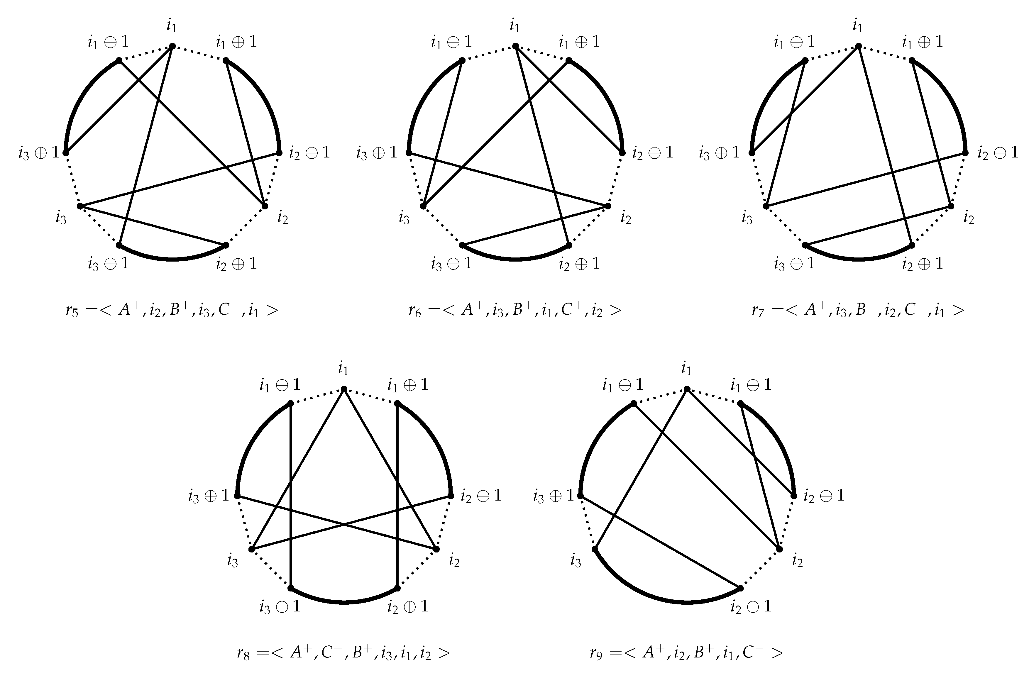
The ideas outlined for the 3-OPT neighborhood and the corresponding successful computational results have prompted us to investigate the possibility of speeding up in a similar way some other type of cubic moves. In this section, we just give a few examples to show that indeed this can be done.

Consider, for instance, some special types of K-OPT moves (where $K>3$ edges are taken out from the tour and replaced by K new edges) in which the removed edges are identified by three indexes $i_1,i_2,i_3$. For instance, let $K=6$ and the removed edges be

$$\{i_1\ominus 1,i_1\},\{i_1,i_1\oplus 1\},\{i_2\ominus 1,i_2\},\{i_2,i_2\oplus 1\},\{i_3\ominus 1,i_3\},\{i_3,i_3\oplus 1\}.$$

The tour is then reconnected in any way that excludes the removed edges (clearly there are many possibilities, we’ll just look at a few). To describe the way in which the tour is reconnected we can still use the concept of the reinsertion scheme. Let us describe the tour before the move (by default, clockwise) as

$$A,i_1,B,i_2,C,i_3,$$

where $A=(i_3\oplus 1,\dots ,i_1\ominus 1)$, $B=(i_1\oplus 1,\dots ,i_2\ominus 1)$ and $C=(i_2\oplus 1,\dots ,i_3\ominus 1)$. In the new tour, each segment $X\in \{A,B,C\}$ can be traversed clockwise (denoted by $X^{+}$) or counter-clockwise (denoted by $X^{-}$). A reinsertion scheme is then a permutation of $\{A^{+},B,C,i_1,i_2,i_3\}$, starting with $A^{+}$ (we adopt the convention that A is always the first segment and is always traversed clockwise) and with B and C signed either ’+’ or ’-’. Let us first consider two simple examples of reinsertion schemes, i.e., those in which the move maintains the pattern “segment, node, segment, node, segment, node” and the segments keep the clockwise orientation and the original order (i.e., $A^{+}$, $B^{+}$, $C^{+}$). This leaves only two possible reinsertion schemes for the true moves (as many as the derangements of $\{1,2,3\}$), namely (see Figure 4)

$$r_5:=<A^{+},i_2,B^{+},i_3,C^{+},i_1>$$

$$r_6:=<A^{+},i_3,B^{+},i_1,C^{+},i_2>$$

The value of a move $((i_1,i_2,i_3),r_5)$ is $\Delta ((i_1,i_2,i_3),r_5)=$

$$\begin{array}{cc}\hfill =& \left[c(i_1\ominus 1,i_1)+c(i_1,i_1\oplus 1)+c(i_2\ominus 1,i_2)+c(i_2,i_2\oplus 1)+c(i_3\ominus 1,i_3)+c(i_3,i_3\oplus 1)\right]-\hfill \\ \hfill & \left[c(i_1,i_3\ominus 1)+c(i_1,i_3\oplus 1)+c(i_2,i_1\ominus 1)+c(i_2,i_1\oplus 1)+c(i_3,i_2\ominus 1)+c(i_3,i_2\oplus 1)\right]\hfill \\ \hfill =& [{\tau }^{+}(i_2,i_1)+{\tau }^{-}(i_2,i_1)]+[{\tau }^{+}(i_3,i_2)+{\tau }^{-}(i_3,i_2)]+[{\tau }^{+}(i_1,i_3)+{\tau }^{-}(i_1,i_3)]\hfill \end{array}$$

So we have

$$\Delta ((i_1,i_2,i_3),r_5)=f_{r_5}^{12}(i_1,i_2)+f_{r_5}^{23}(i_2,i_3)+f_{r_5}^{13}(i_1,i_3)$$

if we define the three functions $f_r^{\alpha }$ to be

• $f_{r_5}^{12}:(x,y)\in {\mathcal{S}}_{12}\mapsto {\tau }^{+}(y,x)+{\tau }^{-}(y,x)$
• $f_{r_5}^{23}:(x,y)\in {\mathcal{S}}_{23}\mapsto {\tau }^{+}(y,x)+{\tau }^{-}(y,x)$
• $f_{r_5}^{13}:(x,y)\in {\mathcal{S}}_{13}\mapsto {\tau }^{+}(x,y)+{\tau }^{-}(x,y)$

Similarly, a move $((i_1,i_2,i_3),r_6)$ has value $\Delta ((i_1,i_2,i_3),r_6)=$

$$\begin{array}{cc}\hfill =& \left[c(i_1\ominus 1,i_1)+c(i_1,i_1\oplus 1)+c(i_2\ominus 1,i_2)+c(i_2,i_2\oplus 1)+c(i_3\ominus 1,i_3)+c(i_3,i_3\oplus 1)\right]-\hfill \\ \hfill & \left[c(i_1,i_2\ominus 1)+c(i_1,i_2\oplus 1)+c(i_2,i_3\ominus 1)+c(i_2,i_3\oplus 1)+c(i_3,i_1\ominus 1)+c(i_3,i_1\oplus 1)\right]\hfill \\ \hfill =& [{\tau }^{+}(i_1,i_2)+{\tau }^{-}(i_1,i_2)]+[{\tau }^{+}(i_2,i_3)+{\tau }^{-}(i_2,i_3)]+[{\tau }^{+}(i_3,i_1)+{\tau }^{-}(i_3,i_1)]\hfill \\ \hfill =& f_{r_6}^{12}(i_1,i_2)+f_{r_6}^{23}(i_2,i_3)+f_{r_6}^{13}(i_1,i_3),\hfill \end{array}$$

where we have defined the three functions $f_r^{\alpha }$ as

• $f_{r_6}^{12}:(x,y)\in {\mathcal{S}}_{12}\mapsto {\tau }^{+}(x,y)+{\tau }^{-}(x,y)$
• $f_{r_6}^{23}:(x,y)\in {\mathcal{S}}_{23}\mapsto {\tau }^{+}(x,y)+{\tau }^{-}(x,y)$
• $f_{r_6}^{13}:(x,y)\in {\mathcal{S}}_{13}\mapsto {\tau }^{+}(y,x)+{\tau }^{-}(y,x)$

Let us now consider the case of the above move when we keep the order A, B, C, but we also allow for reversing either B or C. It turns out that, over all the signings of B and C and permutations of $i_1,i_2,i_3$, there is only one possible reinsertion scheme, namely (see Figure 4)

$$r_7:=<A^{+},i_3,B^{-},i_2,C^{-},i_1>.$$

The value of a move $((i_1,i_2,i_3),r_7)$ is $\Delta ((i_1,i_2,i_3),r_7)=$

$$\begin{array}{cc}\hfill =& \left[c(i_1\ominus 1,i_1)+c(i_1,i_1\oplus 1)+c(i_2\ominus 1,i_2)+c(i_2,i_2\oplus 1)+c(i_3\ominus 1,i_3)+c(i_3,i_3\oplus 1)\right]-\hfill \\ \hfill & \left[c(i_1,i_2\oplus 1)+c(i_1,i_3\oplus 1)+c(i_2,i_1\oplus 1)+c(i_2,i_3\ominus 1)+c(i_3,i_1\ominus 1)+c(i_3,i_2\ominus 1)\right]\hfill \\ \hfill =& [{\tau }^{+}(i_1,i_2)+{\tau }^{+}(i_2,i_1)]+[{\tau }^{-}(i_2,i_3)+{\tau }^{-}(i_3,i_2)]+[{\tau }^{+}(i_1\ominus 1,i_3\ominus 1)+{\tau }^{-}(i_3\oplus 1,i_1\oplus 1)]\hfill \\ \hfill =& f_{r_7}^{12}(i_1,i_2)+f_{r_7}^{23}(i_2,i_3)++f_{r_7}^{13}(i_1,i_3),\hfill \end{array}$$

where we have defined the three functions $f_r^{\alpha }$ as

• $f_{r_7}^{12}:(x,y)\in {\mathcal{S}}_{12}\mapsto {\tau }^{+}(x,y)+{\tau }^{+}(y,x)$
• $f_{r_7}^{23}:(x,y)\in {\mathcal{S}}_{23}\mapsto {\tau }^{-}(x,y)+{\tau }^{-}(y,x)$
• $f_{r_7}^{13}:(x,y)\in {\mathcal{S}}_{13}\mapsto {\tau }^{+}(x\ominus 1,y\ominus 1)+{\tau }^{-}(y\oplus 1,x\oplus 1)$

Finally, let us consider one last example of these special 6-OPT moves, in which we rearrange the permutation of segments and nodes, namely (see Figure 4)

$$r_8:=<A^{+},C^{-},B^{+},i_3,i_1,i_2>.$$

The value of a move $((i_1,i_2,i_3),r_8)$ is $\Delta ((i_1,i_2,i_3),r_8)=$

$$\begin{array}{cc}\hfill =& \left[c(i_1\ominus 1,i_1)+c(i_1,i_1\oplus 1)+c(i_2\ominus 1,i_2)+c(i_2,i_2\oplus 1)+c(i_3\ominus 1,i_3)+c(i_3,i_3\oplus 1)\right]-\hfill \\ \hfill & \left[c(i_1\ominus 1,i_3\ominus 1)+c(i_1,i_3)+c(i_2\ominus 1,i_3)+c(i_2,i_3\oplus 1)+c(i_1,i_2)+c(i_1\oplus 1,i_2\oplus 1)\right]\hfill \\ \hfill =& [{\tau }^{-}(i_1\oplus 1,i_2\oplus 2)+{\tau }^{-}(i_2,i_1\oplus 1)]+[{\tau }^{+}(i_2,i_3)+{\tau }^{-}(i_3,i_2)]+[{\tau }^{+}(i_1\ominus 1,i_3\ominus 2)+{\tau }^{+}(i_3,i_1\ominus 1)]\hfill \\ \hfill =& f_{r_8}^{12}(i_1,i_2)+f_{r_8}^{23}(i_2,i_3)++f_{r_8}^{13}(i_1,i_3),\hfill \end{array}$$

where we have defined the three functions $f_r^{\alpha }$ as

• $f_{r_8}^{12}:(x,y)\in {\mathcal{S}}_{12}\mapsto {\tau }^{-}(x\oplus 1,y\oplus 2)+{\tau }^{-}(y,x\oplus 1)$
• $f_{r_8}^{23}:(x,y)\in {\mathcal{S}}_{23}\mapsto {\tau }^{+}(x,y)+{\tau }^{-}(y,x)$
• $f_{r_8}^{13}:(x,y)\in {\mathcal{S}}_{13}\mapsto {\tau }^{+}(x\ominus 1,y\ominus 2)+{\tau }^{+}(y,x\ominus 1)$

To finish this section let us consider another type of cubic move, for example, a special 5-OPT move. In particular, let the removed edges be

$$\{i_1\ominus 1,i_1\},\{i_1,i_1\oplus 1\},\{i_2\ominus 1,i_2\},\{i_2,i_2\oplus 1\},\{i_3,i_3\oplus 1\}.$$

The tour is then reconnected in any way that excludes the removed edges (clearly there are many possibilities, we will just look at one of them). By using the previous notation for the reinsertion schemes, let us consider the scheme (see Figure 4)

$$r_9:=<A^{+},i_2,B^{+},i_1,C^{-}>.$$

The value of a move $((i_1,i_2,i_3),r_9)$ is $\Delta ((i_1,i_2,i_3),r_9)=$

$$\begin{array}{cc}\hfill =& \left[c(i_1\ominus 1,i_1)+c(i_1,i_1\oplus 1)+c(i_2\ominus 1,i_2)+c(i_2,i_2\oplus 1)+c(i_3,i_3\oplus 1)\right]-\hfill \\ \hfill & \left[c(i_1\ominus 1,i_2)+c(i_1,i_2\ominus 1)+c(i_1\oplus 1,i_2)+c(i_2\oplus 1,i_3\oplus 1)+c(i_3,i_1)\right]\hfill \\ \hfill =& [{\tau }^{-}(i_1\oplus 1,i_2\oplus 1)+{\tau }^{+}(i_1\ominus 1,i_2\ominus 1)+{\tau }^{+}(i_2\ominus 1,i_1\ominus 1)]+{\tau }^{-}(i_2\oplus 1,i_3+2)+{\tau }^{+}(i_3,i_1\ominus 1)\hfill \\ \hfill =& f_{r_9}^{12}(i_1,i_2)+f_{r_9}^{23}(i_2,i_3)+f_{r_9}^{13}(i_1,i_3),\hfill \end{array}$$

where we have defined the three functions $f_r^{\alpha }$ as

• $f_{r_9}^{12}:(x,y)\in {\mathcal{S}}_{12}\mapsto {\tau }^{-}(x\oplus 1,y\oplus 1)+{\tau }^{+}(x\ominus 1,y\ominus 1)+{\tau }^{+}(y\ominus 1,x\ominus 1)$
• $f_{r_9}^{23}:(x,y)\in {\mathcal{S}}_{23}\mapsto {\tau }^{-}(x\oplus 1,y\oplus 2)$
• $f_{r_9}^{13}:(x,y)\in {\mathcal{S}}_{13}\mapsto {\tau }^{+}(y,x\ominus 1)$

It should be clear that, to find the best move of the special types described in this section, we can put the partial moves in a heap and use the same strategy we have developed in Section 4. The algorithm is the same as before, with the difference that in line 2 of procedure BuildHeap we iterate over the schemes $r_5,\dots ,r_9$ instead of $r_1,\dots ,r_4$.

7. Conclusions

In this work, we have described an algorithmic strategy for optimizing the 3-OPT neighborhood in an effective way. Our strategy relies on a particular order of enumeration of the triples which allows us to find the best 3-OPT move without having to consider all the possibilities. This is achieved by a pruning rule and by the use of the max-heap as a suitable data structure for finding in a quick way good candidates for the best move.

Extensive computational experiments prove that this strategy largely outperforms the classical $\mathsf{\Theta }\left(n^3\right)$ “nested-for” approach on average. In particular, our approach exhibits a time complexity bounded by $O\left(n^{2.5}\right)$ on various types of random graphs.

The goal of our work was to show how the use of the 3-OPT neighborhood can be extended to graphs of much larger size than before. We did not try to assess the effectiveness of this neighborhood in finding good-quality tours, nor possible refinements to 3-OPT local search (such as restarts, perturbations, the effectiveness of the other type of 3-OPT moves we introduced, etc.). These types of investigations would have required a large set of experiments and further coding, and can be the matter of future research. We also leave to further investigation the possibility of using our type of enumeration strategy for other polynomial-size neighborhoods, including some for different problems than the TSP. In this respect, we have obtained some promising preliminary results for the application of our approach to the 4-OPT neighborhood [17].

Perhaps the main open question deriving from our work is to prove that the expected time complexity of our algorithm is subcubic on, for instance, uniform random graphs. Note that the problem of finding the best 3-OPT move is the same as that of finding the largest triangle in a complete graph with suitable edge lengths $L_{ij}$. For instance, for the reinsertion scheme $r_1$ in (4), the length of an edge $(i,j)$ is $L_{ij}:={\tau }^{+}(i,j)=c(i,i\oplus 1)-c(i,j\oplus 1)$. For a random TSP instance, each random variable $L_{ij}$ is therefore the difference of two uniform random variables, and this definitely complicates a probabilistic analysis of the algorithm. If one makes the simplifying assumption that the lengths $L_{ij}$ are independent uniform random variables drawn in $[0,1]$, then it can be shown that finding the largest triangle in a graph takes quadratic time on average, and this already requires a quite complex proof [18]. However, since in our case the variables $L_{ij}$ are not independent, nor uniformly distributed, we were not able to prove that the expected running time is subcubic, and such a proof appears very difficult to obtain.