Translating Workflow Nets to Process Trees: An Algorithmic Approach


Abstract
1. Introduction
2. Preliminaries
2.1. Basic Notation
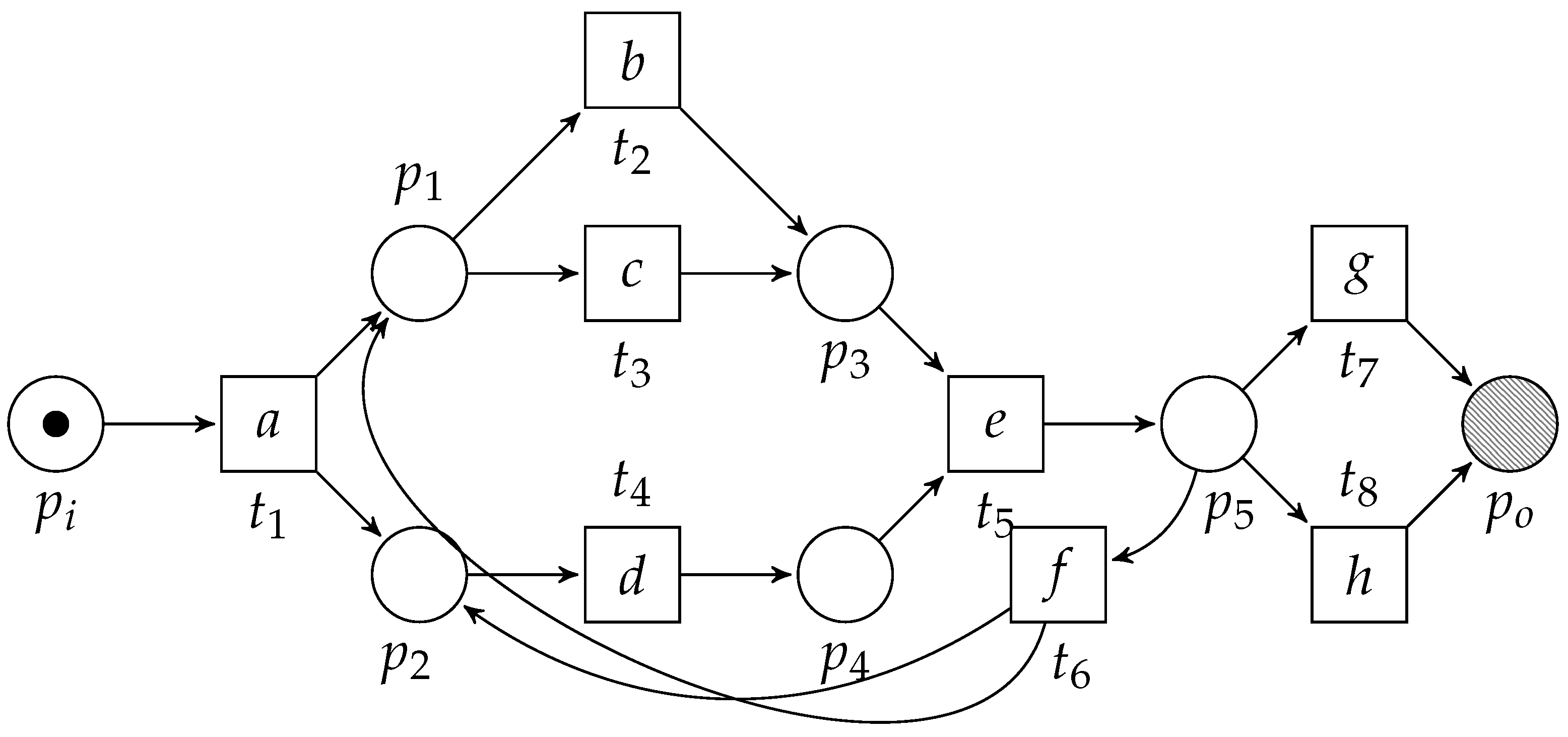
2.2. Workflow Nets
- 1.
- ;is the unique source place.
- 2.
- ;is the unique sink place.
- 3.
- Each elementis on a path fromto.
- 1.
- is safe,i.e., ,
- 2.
- can always be reached, i.e.,.
- 3.
- Eachis enabled, at some point, i.e.,.
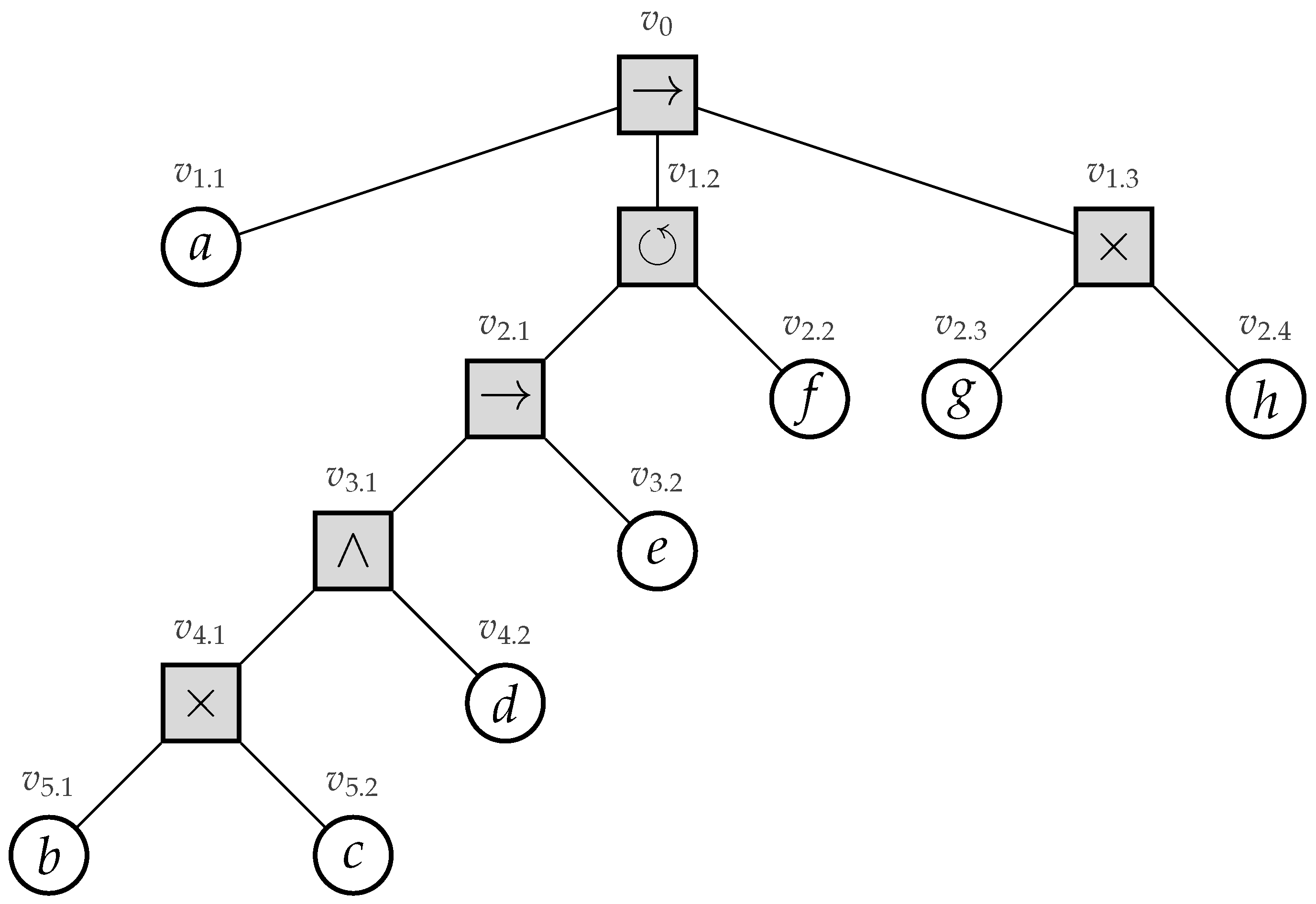
2.3. Process Trees
- 1.
- ; an (non-observable) activity,
- 2.
- , for, , whereare process trees;
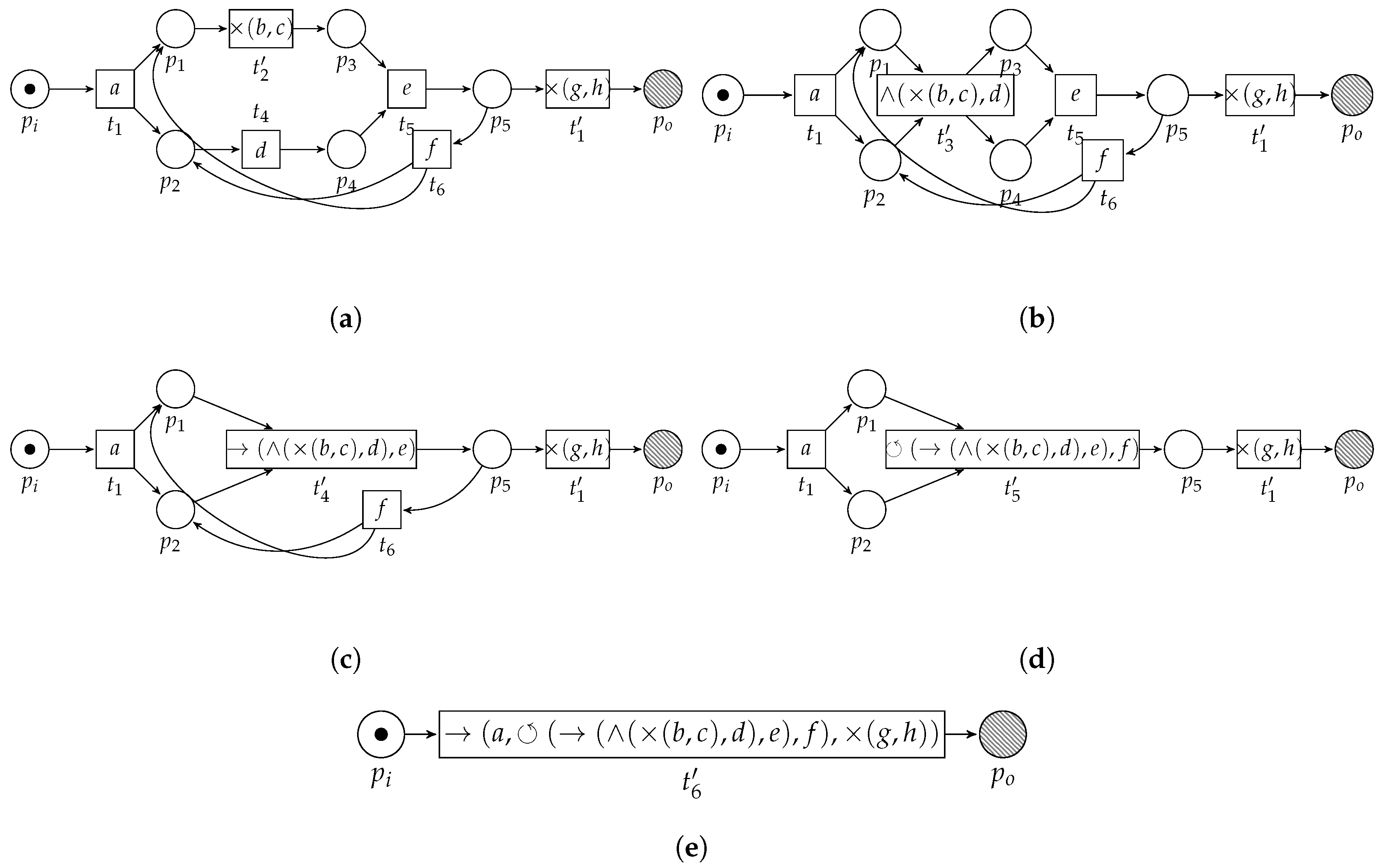
3. Translating Workflow Nets to Process Trees
3.1. Overview
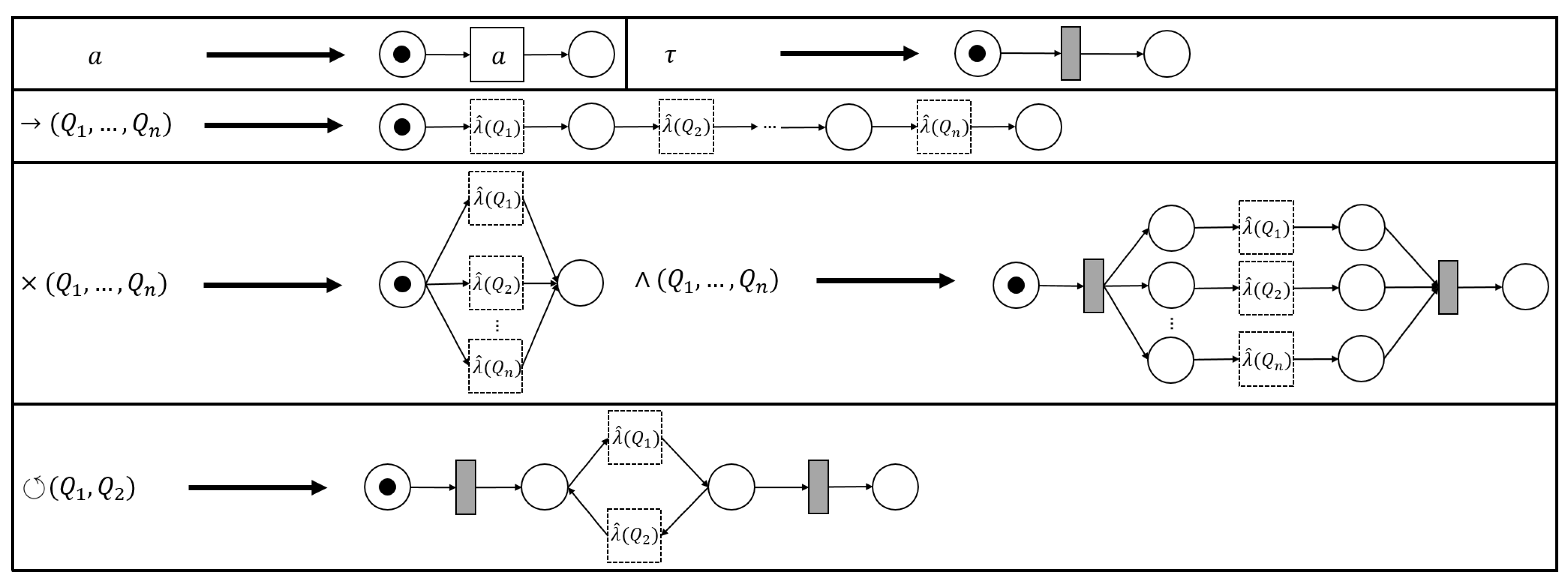
3.2. PTree-Nets and Their Unfolding
- 1.
- ,
- 2.
- ,
- 3.
- ,
- 4.
- . (Since functions are binary Cartesian products, we write set operations here).
3.3. Pattern Reduction
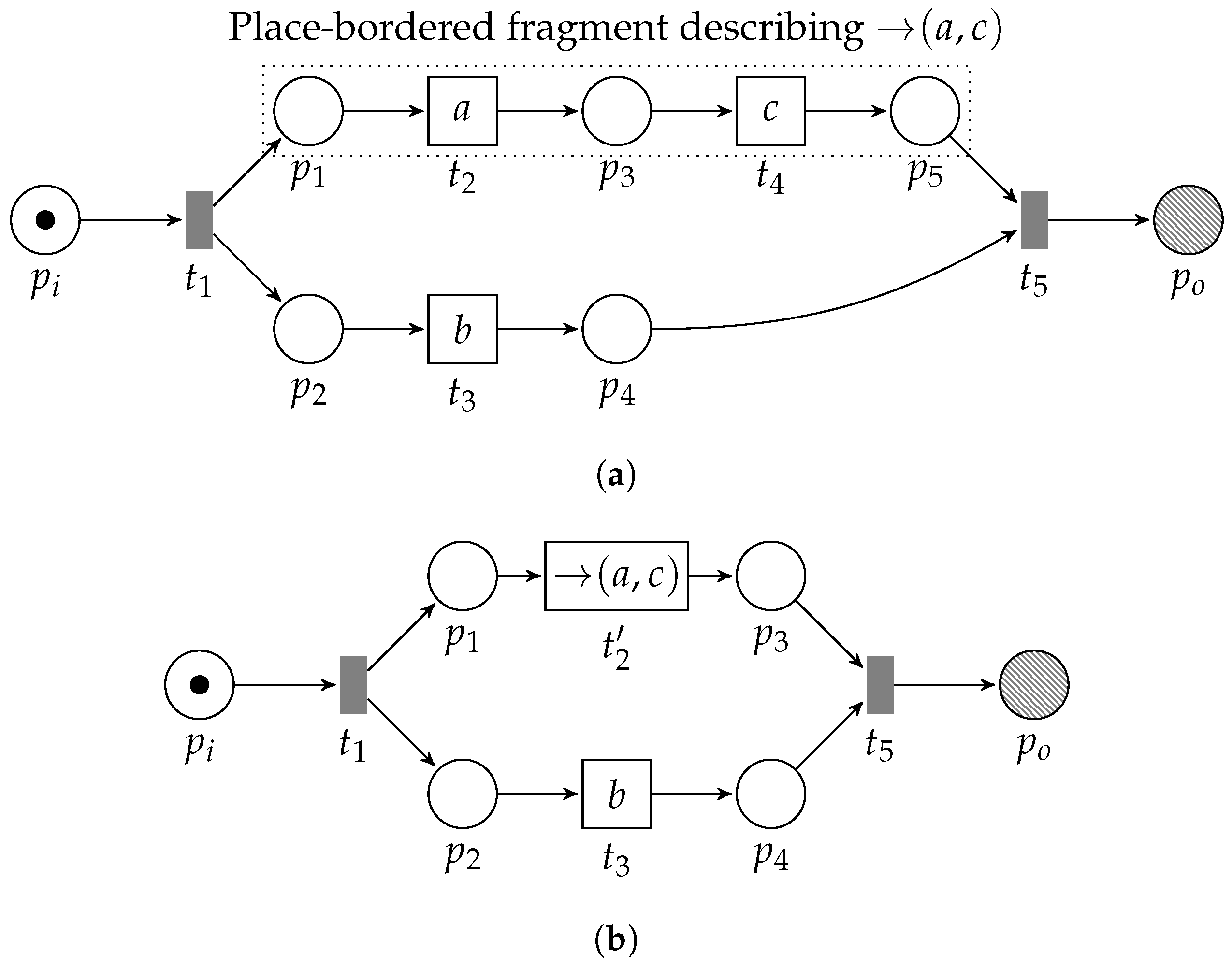
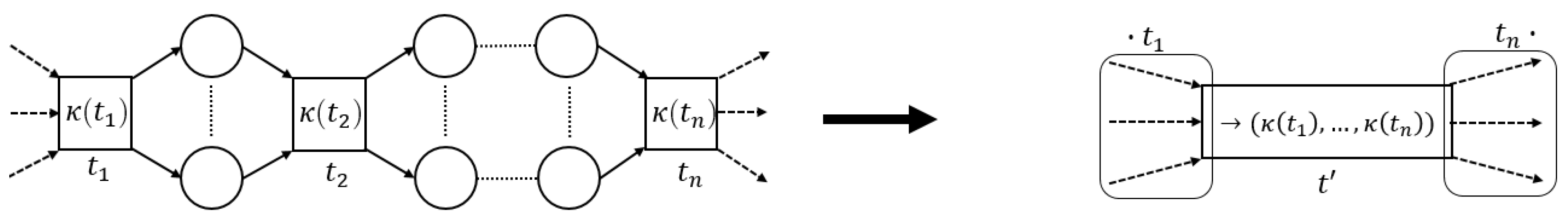
3.3.1. Sequential Pattern
- 1.
- , transitionenables; and
- 2.
- , enabling is unique,
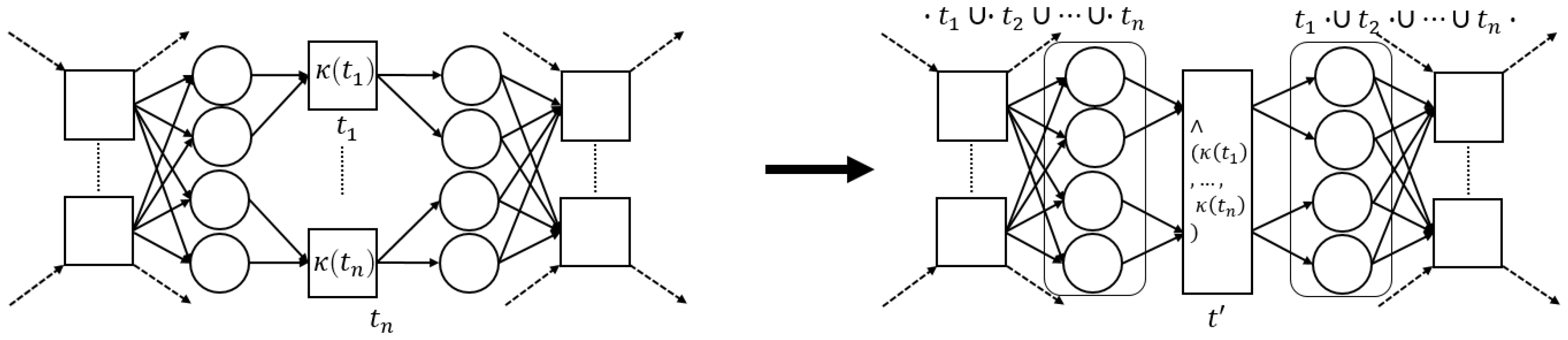
3.3.2. Exclusive Choice Pattern
- 1.
- , all pre-sets are shared among the members of the pattern;
- 2.
- , all post-sets are shared among the members of the pattern; and
- 3.
- , self-loops are not allowed,
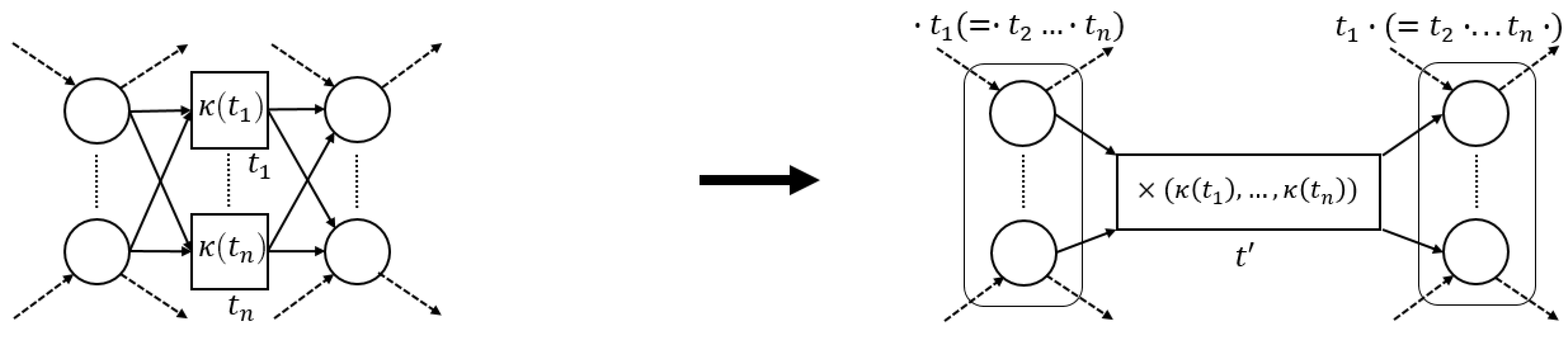
3.3.3. Concurrent Pattern
- 1.
- , no interaction between the member’s pre-sets;
- 2.
- , no interaction between the member’s post-sets;
- 3.
- , pre-set places uniquely connect to a member;
- 4.
- , post-set places uniquely connect to a member;
- 5.
- , members do not influence other members;
- 6.
- , member’s pre-sets share their pre-set;
- 7.
- , member firing does not affect other members;
- 8.
- , member’s post-sets share their post-set;
- 9.
- , pre-sets of enablers are equal;
- 10.
- , post-sets of enablers are equal,
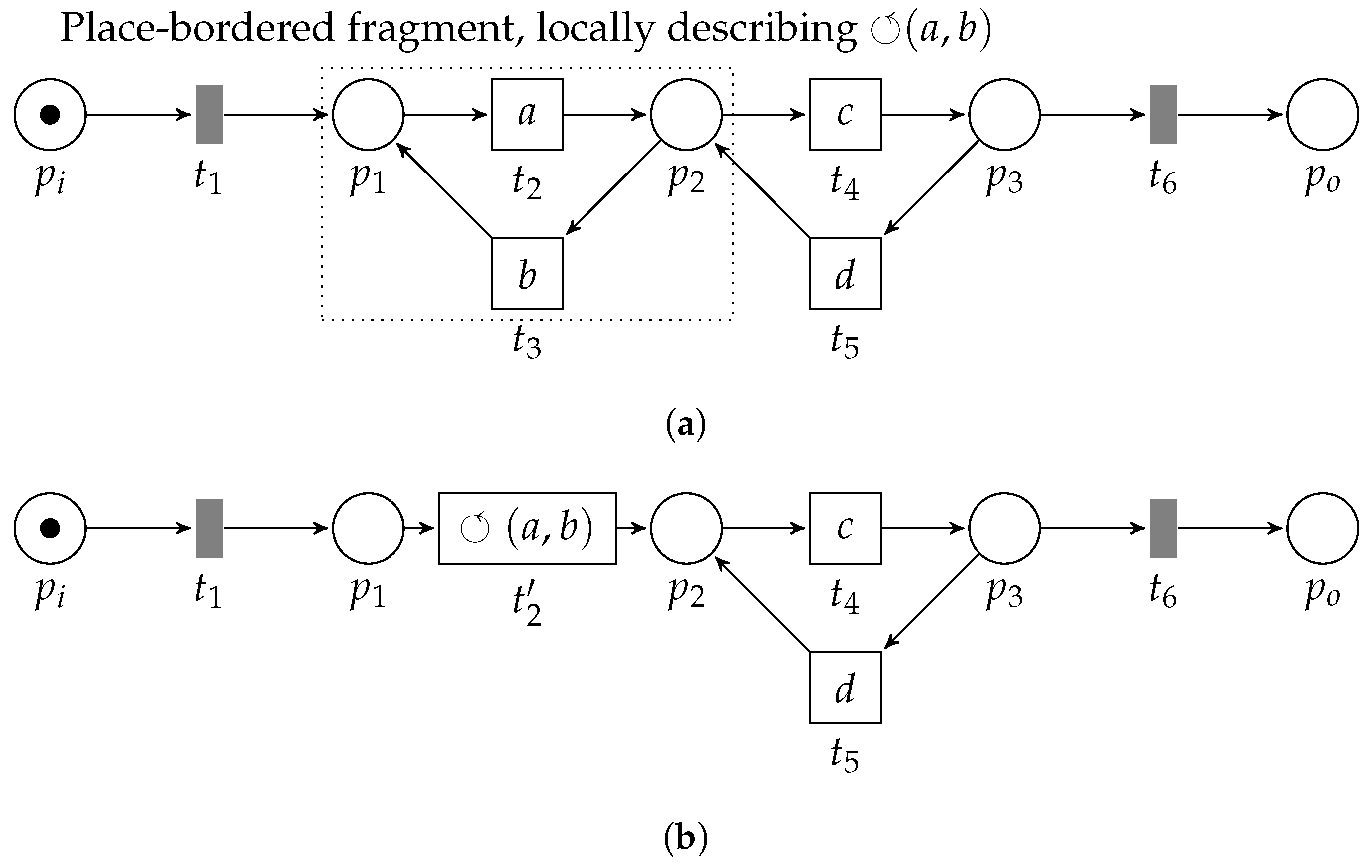
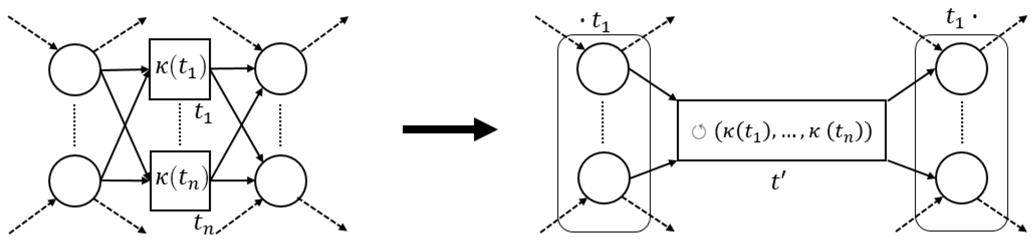
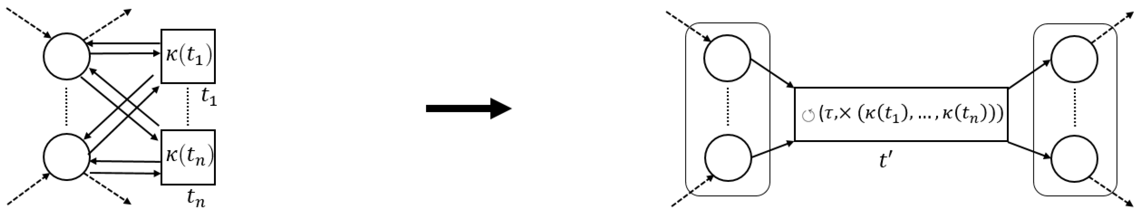
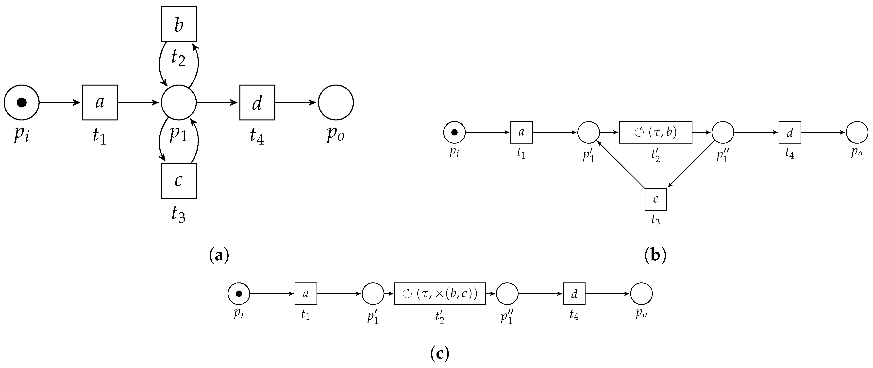
3.3.4. Loop Pattern
- 1.
- , pre-set ofis the post-set of;
- 2.
- , pre-set ofis the post-set of;
- 3.
- , is the only transition in the post-set of its pre-set;
- 4.
- ; , is the only transition in the pre-set of its post-set,
3.4. Algorithm
| Algorithm 1: WF-net reduction |
 |
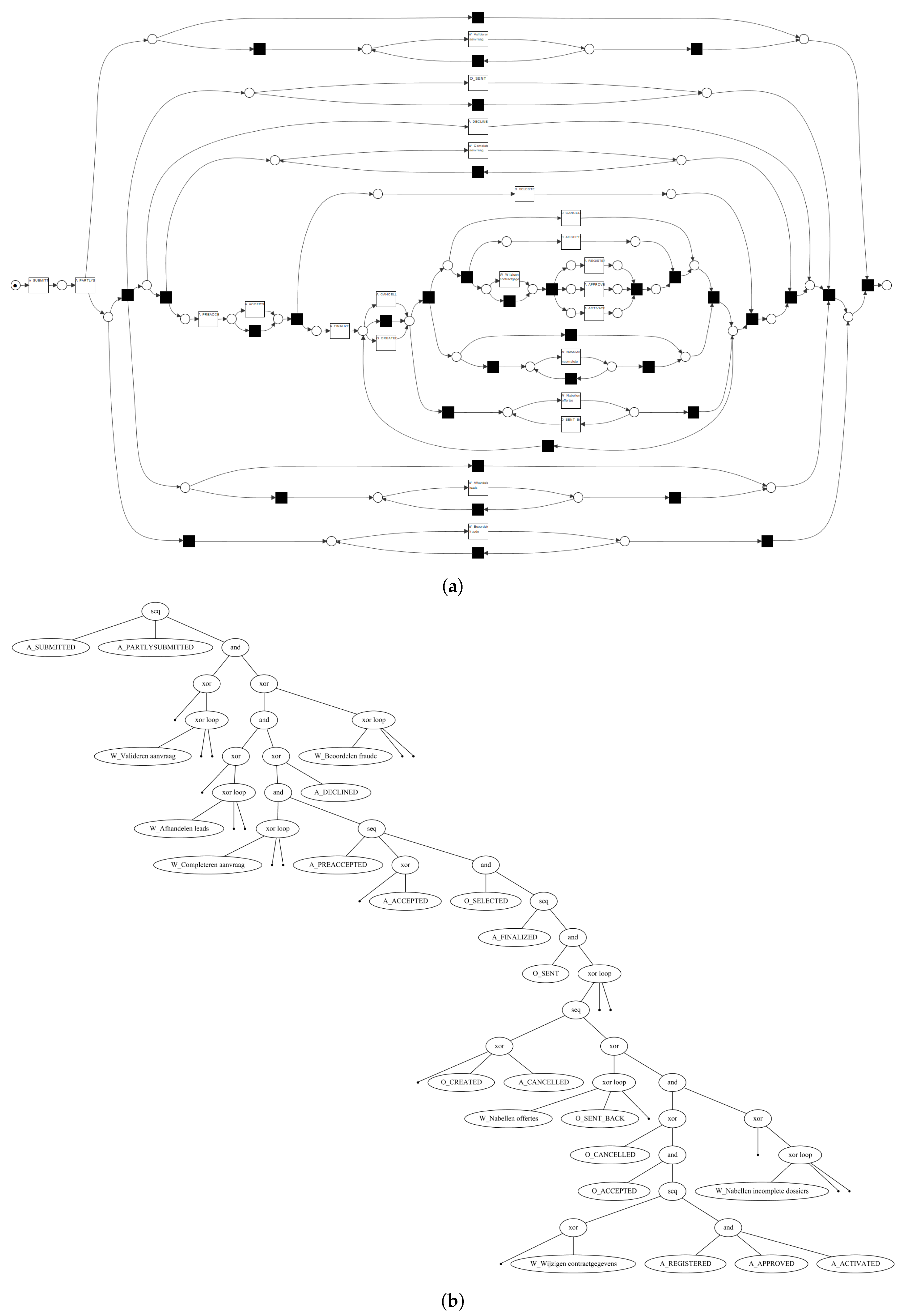
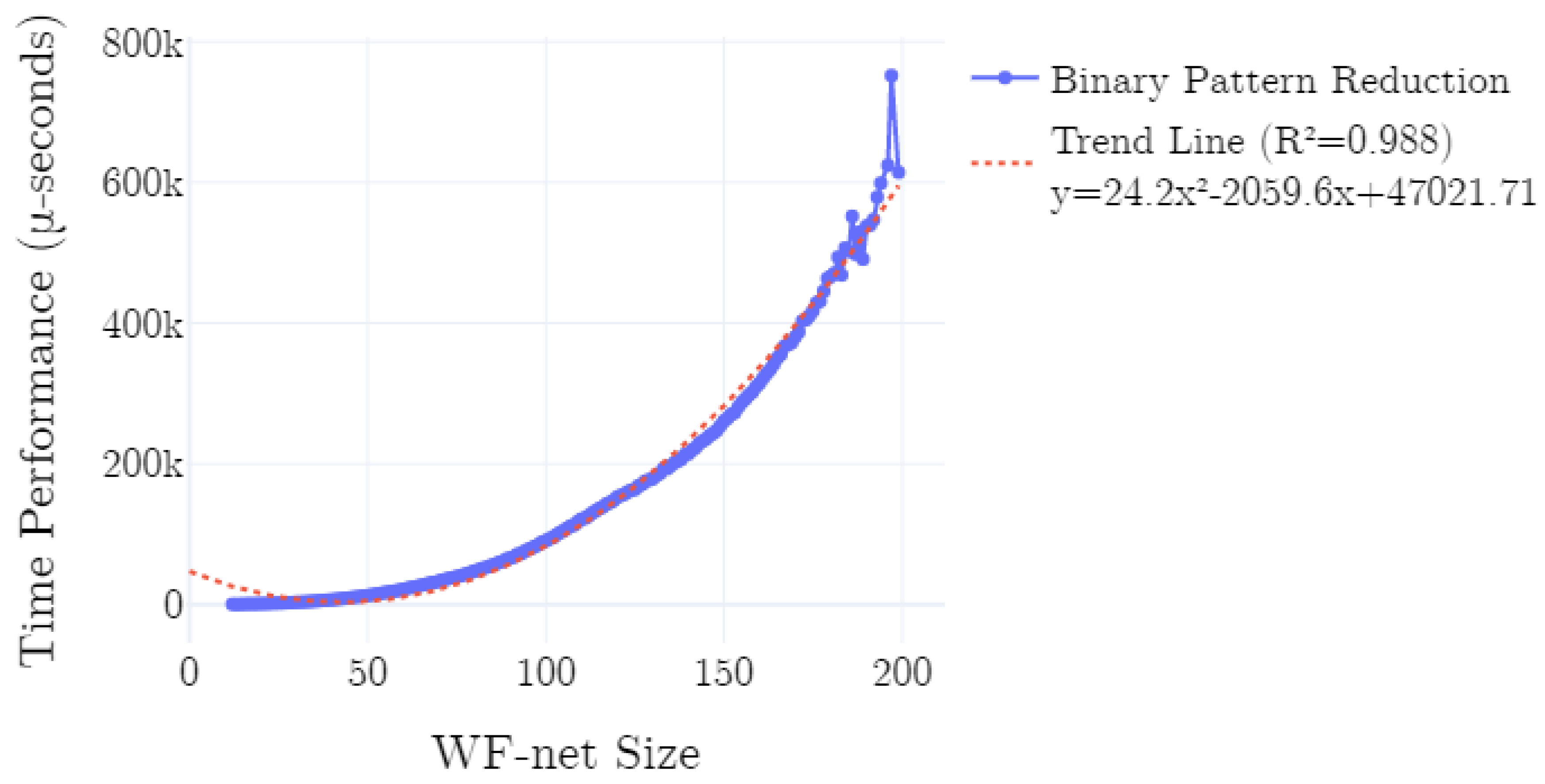
4. Evaluation
4.1. Implementation
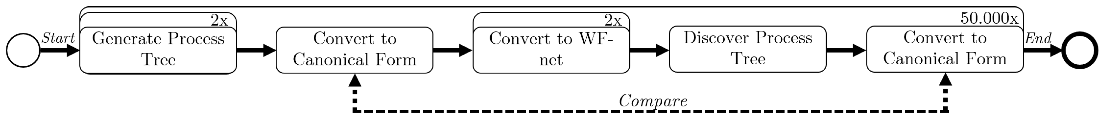
4.2. Experimental Setup
4.3. Results
5. Related Work
6. Discussion
6.1. Extensibility
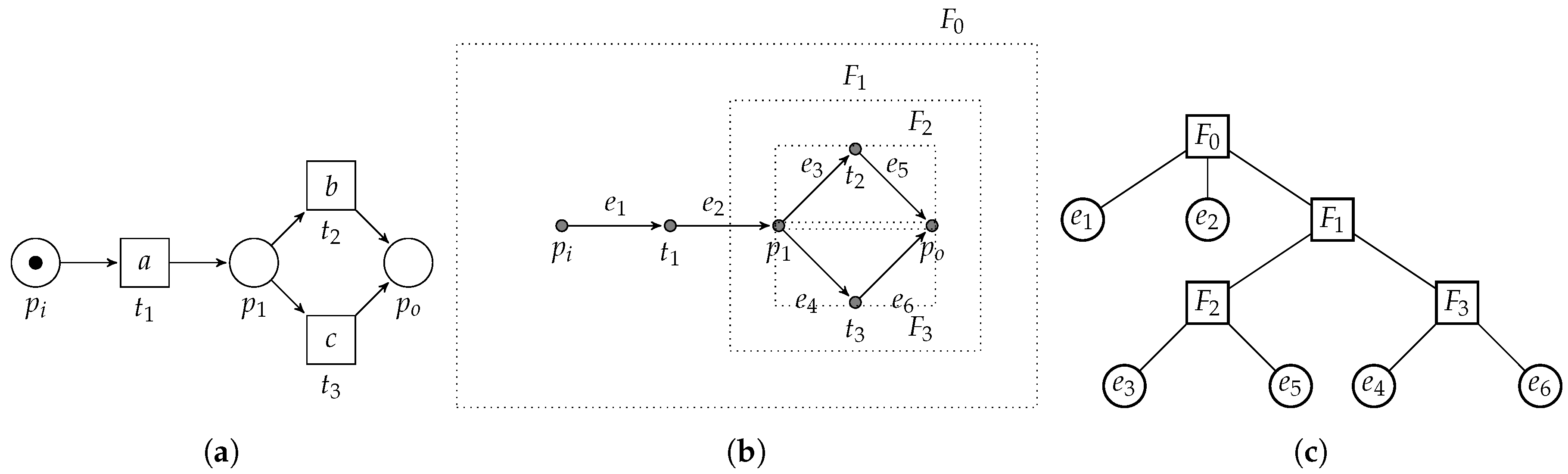
6.2. Relation to Refined Process Structure Tree
6.3. Reducibility of WF-Nets
7. Conclusions
Author Contributions
Funding
Conflicts of Interest
References
- van der Aalst, W.M.P. Process Mining—Data Science in Action, 2nd ed.; Springer: New York, NY, USA, 2016. [Google Scholar]
- Dijkman, R.M.; Dumas, M.; Ouyang, C. Semantics and analysis of business process models in BPMN. Inf. Softw. Technol. 2008, 50, 1281–1294. [Google Scholar] [CrossRef]
- van der Aalst, W.M.P. Formalization and verification of event-driven process chains. Inf. Softw. Technol. 1999, 41, 639–650. [Google Scholar] [CrossRef]
- van der Aalst, W.M.P.; Buijs, J.C.A.M.; van Dongen, B.F. Towards Improving the Representational Bias of Process Mining. In Proceedings of the SIMPDA, Campione d’Italia, Italy, 29 June–1 July 2011; pp. 39–54. [Google Scholar]
- Lee, W.L.J.; Verbeek, H.M.W.; Munoz-Gama, J.; van der Aalst, W.M.P.; Sepúlveda, M. Recomposing conformance: Closing the circle on decomposed alignment-based conformance checking in process mining. Inf. Sci. 2018, 466, 55–91. [Google Scholar] [CrossRef]
- van Zelst, S.J.; Bolt, A.; van Dongen, B.F. Computing Alignments of Event Data and Process Models. ToPNoC 2018, 13, 1–26. [Google Scholar]
- Schuster, D.; van Zelst, S.J.; van der Aalst, W.M.P. Alignment Approximation for Process Trees (forthcoming). In Proceedings of the 5th International Workshop on Process Querying, Manipulation, and Intelligence (PQMI 2020), Padua, Italy, 18 August 2020. [Google Scholar]
- van der Aalst, W.M.P.; de Medeiros, A.K.A.; Weijters, A.J.M.M. Process Equivalence: Comparing Two Process Models Based on Observed Behavior. In Proceedings of the Business Process Management, 4th International Conference, BPM 2006, Vienna, Austria, 5–7 September 2006; pp. 129–144. [Google Scholar]
- van Dongen, B.F.; Dijkman, R.M.; Mendling, J. Measuring Similarity between Business Process Models. In Seminal Contributions to Information Systems Engineering, 25 Years of CAiSE; Krogstie, J., Pastor, O., Pernici, B., Rolland, C., Sølvberg, A., Eds.; Springer: New York, NY, USA, 2013; pp. 405–419. [Google Scholar]
- Mendling, J.; Lassen, K.B.; Zdun, U. On the transformation of control flow between block-oriented and graph-oriented process modelling languages. IJBPIM 2008, 3, 96–108. [Google Scholar] [CrossRef]
- Berti, A.; van Zelst, S.J.; van der Aalst, W.M.P. Process Mining for Python (PM4Py): Bridging the Gap Between Process-and Data Science. In Proceedings of the ICPM Demo Track 2019, Aachen, Germany, 24–26 June 2019; pp. 13–16. [Google Scholar]
- Leemans, S.J.J.; Fahland, D.; van der Aalst, W.M.P. Discovering Block-Structured Process Models from Event Logs—A Constructive Approach. In Proceedings of the Application and Theory of Petri Nets and Concurrency—34th International Conference, Milan, Italy, 24–28 June 2013; pp. 311–329. [Google Scholar]
- Verbeek, E.; Buijs, J.C.A.M.; van Dongen, B.F.; van der Aalst, W.M.P. ProM 6: The Process Mining Toolkit. In Proceedings of the Business Process Management 2010 Demonstration Track, Hoboken, NJ, USA, 14–16 September 2010. [Google Scholar]
- van Dongen, B.F. BPI Challenge 2012; Eindhoven University of Technology: Eindhoven, The Netherlands, 2012. [Google Scholar] [CrossRef]
- van der Aalst, W.M.P. The Application of Petri Nets to Workflow Management. J. Circuits Syst. Comput. 1998, 8, 21–66. [Google Scholar] [CrossRef]
- Murata, T. Petri nets: Properties, analysis and applications. Proc. IEEE 1989, 77, 541–580. [Google Scholar] [CrossRef]
- van der Aalst, W.M.P. Workflow Verification: Finding Control-Flow Errors Using Petri-Net-Based Techniques. In Proceedings of the Business Process Management, Models, Techniques, and Empirical Studies, Berlin, Germany, 19 April 2000; pp. 161–183. [Google Scholar]
- Jouck, T.; Depaire, B. PTandLogGenerator: A Generator for Artificial Event Data. In Proceedings of the BPM Demo Track 2016, Rio de Janeiro, Brazil, 21 September 2016; pp. 23–27. [Google Scholar]
- Jouck, T.; Depaire, B. Generating Artificial Data for Empirical Analysis of Control-flow Discovery Algorithms—A Process Tree and Log Generator. Bus. Inf. Syst. Eng. 2019, 61, 695–712. [Google Scholar] [CrossRef]
- Leemans, S. Robust Process Mining with Guarantees. Ph.D. Thesis, Department of Mathematics and Computer Science, Eindhoven University of Technology, Eindhoven, The Netherlands, 2017. [Google Scholar]
- Augusto, A.; Conforti, R.; Dumas, M.; Rosa, M.L.; Maggi, F.M.; Marrella, A.; Mecella, M.; Soo, A. Automated Discovery of Process Models from Event Logs: Review and Benchmark. IEEE Trans. Knowl. Data Eng. 2019, 31, 686–705. [Google Scholar] [CrossRef]
- Carmona, J.; van Dongen, B.F.; Solti, A.; Weidlich, M. Conformance Checking—Relating Processes and Models; Springer: New York, NY, USA, 2018. [Google Scholar]
- van der Aalst, W.M.P.; Lassen, K.B. Translating unstructured workflow processes to readable BPEL: Theory and implementation. Inf. Softw. Technol. 2008, 50, 131–159. [Google Scholar] [CrossRef]
- Lassen, K.B.; van der Aalst, W.M.P. WorkflowNet2BPEL4WS: A Tool for Translating Unstructured Workflow Processes to Readable BPEL. In Proceedings of the CoopIS, DOA, GADA, and ODBASE, OTM Confederated International Conferences, Montpellier, France, 29 October–3 November 2006; pp. 127–144. [Google Scholar]
- Vanhatalo, J.; Völzer, H.; Koehler, J. The refined process structure tree. Data Knowl. Eng. 2009, 68, 793–818. [Google Scholar] [CrossRef]
- Polyvyanyy, A.; Vanhatalo, J.; Völzer, H. Simplified Computation and Generalization of the Refined Process Structure Tree. In Proceedings of the WS-FM 2010, Hoboken, NJ, USA, 16–17 September 2010; pp. 25–41. [Google Scholar]
- Polyvyanyy, A.; García-Bañuelos, L.; Dumas, M. Structuring Acyclic Process Models. In Proceedings of the Business Process Management—8th International Conference, Hoboken, NJ, USA, 13–16 September 2010; pp. 276–293. [Google Scholar]
- Polyvyanyy, A.; García-Bañuelos, L.; Dumas, M. Structuring acyclic process models. Inf. Syst. 2012, 37, 518–538. [Google Scholar] [CrossRef]
- Polyvyanyy, A.; García-Bañuelos, L.; Fahland, D.; Weske, M. Maximal Structuring of Acyclic Process Models. Comput. J. 2014, 57, 12–35. [Google Scholar] [CrossRef]
- Weidlich, M.; Polyvyanyy, A.; Mendling, J.; Weske, M. Causal Behavioural Profiles—Efficient Computation, Applications, and Evaluation. Fundam. Inform. 2011, 113, 399–435. [Google Scholar] [CrossRef]
- Polyvyanyy, A.; Weidlich, M.; Weske, M. The Biconnected Verification of Workflow Nets. In Proceedings of the On the Move to Meaningful Internet Systems: OTM 2010—Confederated International Conferences: CoopIS, IS, DOA and ODBASE, Hersonissos, Crete, Greece, 25–29 October 2010; pp. 410–418. [Google Scholar]
- Suzuki, I.; Murata, T. A Method for Stepwise Refinement and Abstraction of Petri Nets. J. Comput. Syst. Sci. 1983, 27, 51–76. [Google Scholar] [CrossRef]
- Esparza, J.; Hoffmann, P. Reduction Rules for Colored Workflow Nets. In Proceedings of the Fundamental Approaches to Software Engineering—19th International Conference, FASE 2016, Held as Part of the European Joint Conferences on Theory and Practice of Software, Eindhoven, The Netherlands, 2–8 April 2016; pp. 342–358. [Google Scholar]
- Esparza, J.; Hoffmann, P.; Saha, R. Polynomial analysis algorithms for free choice Probabilistic Workflow Nets. Perform. Evaluation 2017, 117, 104–129. [Google Scholar] [CrossRef]


Publisher’s Note: MDPI stays neutral with regard to jurisdictional claims in published maps and institutional affiliations. |
© 2020 by the authors. Licensee MDPI, Basel, Switzerland. This article is an open access article distributed under the terms and conditions of the Creative Commons Attribution (CC BY) license (http://creativecommons.org/licenses/by/4.0/).
Share and Cite
van Zelst, S.J.; Leemans, S.J.J. Translating Workflow Nets to Process Trees: An Algorithmic Approach. Algorithms 2020, 13, 279. https://doi.org/10.3390/a13110279
van Zelst SJ, Leemans SJJ. Translating Workflow Nets to Process Trees: An Algorithmic Approach. Algorithms. 2020; 13(11):279. https://doi.org/10.3390/a13110279
Chicago/Turabian Stylevan Zelst, Sebastiaan J., and Sander J. J. Leemans. 2020. "Translating Workflow Nets to Process Trees: An Algorithmic Approach" Algorithms 13, no. 11: 279. https://doi.org/10.3390/a13110279
APA Stylevan Zelst, S. J., & Leemans, S. J. J. (2020). Translating Workflow Nets to Process Trees: An Algorithmic Approach. Algorithms, 13(11), 279. https://doi.org/10.3390/a13110279