An EEG Feature Extraction Method Based on Sparse Dictionary Self-Organizing Map for Event-Related Potential Recognition

Abstract

In the application of the brain-computer interface, feature extraction is an important part of Electroencephalography (EEG) signal classification. Using sparse modeling to extract EEG signal features is a common approach. However, the features extracted by common sparse decomposition methods are only of analytical meaning, and cannot relate to actual EEG waveforms, especially event-related potential waveforms. In this article, we propose a feature extraction method based on a self-organizing map of sparse dictionary atoms, which can aggregate event-related potential waveforms scattered inside an over-complete sparse dictionary into the code book of neurons in the self-organizing map network. Then, the cosine similarity between the EEG signal sample and the code vector is used as the classification feature. Compared with traditional feature extraction methods based on sparse decomposition, the classification features obtained by this method have more intuitive electrophysiological meaning. The experiment conducted on a public auditory event-related potential (ERP) brain-computer interface dataset showed that, after the self-organized mapping of dictionary atoms, the neurons’ code vectors in the self-organized mapping network were remarkably similar to the ERP waveform obtained after superposition and averaging. The feature extracted by the proposed method used a smaller amount of data to obtain classification accuracy comparable to the traditional method.

1. Introduction

In the field of biomedical signal processing, accurately finding brain activity from electroencephalography (EEG) signals is the focus of much research. In the brain-computer interface (BCI) applications based on event-related potentials (ERP), fast and efficient feature extraction and classification of EEG signals to understand human intention are the current research hotspots in this field [1]. For the real-world brain-computer interface, it is necessary to extract the ERP waveform from the EEG signal obtained in a single trial [2]. This is not an easy task, since the ERP is usually submerged in noise. Although the commonly used superposition and averaging method can remove part of the random noise, it requires EEG data from multiple trials to be superimposed in order to obtain the results, so the response speed of the entire BCI system cannot be guaranteed, and it cannot be directly applied to real-world BCI. Therefore, it is necessary to use the feature extraction method to extract the classification features from the EEG signal to identify the ERP waveform [3].

1.1. Common EEG Feature Extraction Methods for ERP Classification

At present, one common category of methods is to use temporal characteristics to extract ERP features from EEG. In the year of 1988, Farwell and Donchin proposed stepwise discriminant analysis (SWDA) [4] to extract P300 ERP component from EEG. For multi-channel EEG data, the SWDA method simply combines it to a matrix, without analysis of spatial characteristics. Then, Independent Component Analysis (ICA) was proposed for ERP feature extraction, to overcome the disadvantages of SWDA. ICA can extract the distribution of EEG signals on the brain cortex, and then find the classification features related to ERP. Jung et al. first used ICA to perform spatial analysis on ERP, using the spatial locations to find independent components that can represent ERP, and using them to obtain a more obvious waveform from a single trial [5]; Gao Chang et al. used ICA and the Hilbert-Huang Transform (HHT) [6] combined method to filter artifacts such as the ocular electrogram from the single-channel EEG, and improved the signal-to-noise ratio of ERP [7]. Lee et al. used one-unit ICA with a reference, a variant of ICA for single-trial ERP extraction [8]. By analyzing the spatial distribution difference of each ERP waveform, a more significant difference between the deviation stimulus and the standard stimulus was obtained. Eilbeiigi et al. used global optimal constrained ICA to search for movement-related cortical potential in single-trial EEG data, and reached a higher accuracy rate in a motor-imaging classification experiment [9]. The major shortcoming of the ICA-based methods is that ICA requires separating components to be statistically independent. ICA also needs multi-channel EEG signals for accuracy, which also limits its application in BCI.

Another widely used category of method is based on the statistical characteristics of ERP waveform and noise. Among these methods, component estimation methods based on statistical principles, such as Kalman filtering and Bayesian estimation, can separate ERP waveforms from interference noise, and therefore are used to extract ERP classification features from EEG. Zhang et al. used ICA and Kalman in combination to reduce the interference of white noise on ICA [10] and improve the performance of ICA and ERP extraction; Fukami et al. used Particle Filter to extract P300 waveforms [11], and obtained more accurate delay estimation and P300 component amplitude estimation; Ting et al. used Kalman filter to extract ERP, by adding the EM algorithm to Kalman filter to achieve a more accurate amplitude estimation [12]; Delaney-Busch et al. used Bayesian estimation to study semantic understanding in the process of learning—the trial by trial change of the N400 component in the ERP waveform cannot be achieved by the superimposed average method [13]. Zeyl et al. used Bayesian ranks to analyze and calculate the Event related potential scores of each trial, and use event-related potential scores as the time domain features to improve the accuracy of the P300-based speller [14]. This kind of method can handle delay estimation and amplitude estimation on a single-signal frame and improve the classification accuracy. However, there is a main disadvantage that the non-stationary characteristics of the EEG signals have a negative impact on the performance, so that ERP waveform estimation error cannot be guaranteed.

The third category is feature extraction methods based on sparse modeling. Sparse modeling is an efficient representation method for high-dimensional data, especially for the EEG data [15]. The purpose is to approximate the input data with a linear combination of sparse dictionary atoms. On the other hand, atoms must have data adaptability—that is, atoms can describe certain essential characteristics of the data. At the same time, the linear combination coefficient, also called the sparse representation vector, can also be used as a classification feature. Dai et al. developed a personal identification system using a sparse-modeling-based EEG signal compression-sensing method [16]. Because of the application of sparse modeling and compressed sensing, the amount of data transmission during the operation of the system can be reduced, so that the system can use low-cost wearable EEG acquisition equipment and run on the World Wide Web, which is convenient for application. Wu et al. used Regularized Group Sparse Discriminant Analysis to identify the EEG signal in the brain-computer interface paradigm and identify the P300 waveform in the EEG [17]. Mo et al. directly used sparse representation coefficients as classification features to perform classification in Motor Imagery BCI [18]. Shin et al. added the incoherence measure to the sparse dictionary update process and used this dictionary to sparsely decompose the EEG signal to obtain better classification features [19]. Yuan et al. used kernel sparse representation to sparsely reconstruct EEG data and used sparse reconstruction coefficients as classification features to identify EEG data holding epileptic components [20]. Yu et al. use sparse representation to decompose EEG data for Visual Evoked Potential (VEP) extraction [21]. Shin et al. applied sparse representation to the BCI system of motion imagination and used the Gabor base to construct a dictionary to extract recognizable waveforms from EEG [22]. However, because the definite basis is used, the waveform components are difficult to make accurate and it is impossible to express the nature of the signal.

However, due to the over-completeness of the sparse dictionary, the ERP waveforms in the EEG signal will be distributed among multiple sparse dictionary atoms, which makes it difficult for the sparse reconstruction coefficients to become stable classification features. From the perspective of sparse decomposition theory, since these dictionary atoms are used to perform sparse reconstruction of EEG signals with low errors, these atoms must hold the information needed to identify ERP. Therefore, an extra approach is required to fully utilize ERP waveform information contained in the sparse dictionary atoms for classification features from EEG signals for ERP recognition.

Self-organizing mapping (SOM) is an appropriate approach to solving the problem of scattered ERP in atoms. SOM is a method to produce a typically two-dimensional representation of the input space of the training samples. When the training samples are sparse dictionary atoms, SOM can combine the scattered ERP information into code vectors of the SOM network. SOM was first proposed by Professor T. Kohonen of the University of Helsinki in Finland in 1981 [23,24]. Kohonen believes that when a neural network accepts external input patterns, it will be divided into different corresponding areas, with each area having different response characteristics to the input mode, and this process is completed automatically. SOM is already a common method in the field of biomedical signal analysis and is widely used in the analysis of neural activity data. Ngan et al. used SOM to analyze the time-domain activity waveform of each voxel in Functional magnetic resonance imaging (fMRI) and aggregated the neuron nodes in SOM according to the correlation to find a pattern of voxel activity [25]. Wei et al. used SOM to perform hierarchical cluster analysis of spatio-temporal features on fMRI image data to find fMRI classification features that can represent cognitive activities [26]. Kurth et al. used SOM to perform cluster analysis on EEG signals collected in the clinical scenarios and classify EEG fragments containing epileptic electrical activity and normal EEG fragments [27]. Hemanth et al. first extracted features from EEG signals, and then analyzed the features using SOM to recognize human emotions from EEG [28]. Diaz-Sotelo et al. used SOM to extract features from EEG for a BCI system that can recognize human cognitive states [29]. These studies showed that SOM can be effectively used in the analysis of biological signals, especially brain electrical signals.

1.2. The Proposed Method and Article Structure

In this paper, we propose a feature extraction method based on the self-organizing mapping (SOM) of dictionary atoms. In this method, we first use K-SVD dictionary learning algorithm to construct a sparse dictionary. Then, self-organizing mapping is performed on the dictionary atoms, and the code vector of the neuron is compared with the target ERP waveform as a time-domain waveform. The code vectors with the largest cosine similarity value to the target ERP waveform are found. For the EEG signal frame to be recognized, the cosine similarity between the to-be-recognized frame and the selected code vectors are calculated. These similarity values are the extracted classification features. Finally, the classifier is trained using these features to find the ERP waveform. In the testing phase, the SOM, sparse dictionary, and classifier of the training phase are reused, and the feature extraction operation is repeated for the EEG samples to be recognized. Compared to the three categories of methods mentioned previously, the proposed method has the following advantages: (1) It does not rely on multichannel data. (2) It can deal with non-stationary ERP waveforms. (3) It can make the most use of ERP fragments in sparse dictionary.

This article unfolds as follows: Section 2 provides a brief introduction to EEG sparse decomposition and the procedures of proposed method. In Section 3, the experiment material is explained, and we present the results produced by proposed method. In Section 4 and Section 5, we discussed the advantages of the proposed method and potential further improvements.

2. Methods

2.1. Brief Introduction of EEG Sparse Modeling

The sparse modeling of the signal is the process of representing the signal $\mathit{Y}=\left[{\mathit{y}}_1,{\mathit{y}}_2\dots ,{\mathit{y}}_N\right]\in {\mathbb{R}}_{M\times N}$ by linearly combining the atoms ${\mathit{d}}_k$ in the dictionary $\mathit{D}=\left[{\mathit{d}}_1,{\mathit{d}}_2\dots ,{\mathit{d}}_K\right]\in {\mathbb{R}}_{M\times K}$, as shown in Equation (1).

$$\mathit{Y}=\mathit{DA}+e$$

(1)

In Equation (1), e is the model approximation error, $\mathit{A}=\left[{\mathit{a}}_1,{\mathit{a}}_2\dots ,{\mathit{a}}_N\right]\in {\mathbb{R}}_{K\times N}$ is the sparse coefficient vector. The sparse modeling of the signal can be seen as solving the following optimization problem in Equation (2).

$$\left(P_{(0,\epsilon )}\right)\underset{{\mathbf{a}}_{\mathit{i}}}{min}{∥{\mathbf{a}}_{\mathit{i}}∥}_{0}s.t.{∥{\mathit{y}}_i-{\mathit{Da}}_i∥}_2\le \epsilon$$

(2)

In Equation (2), ${∥\mathit{A}∥}_0$ represents the $l_0$ norm of the sparse coefficient vector $\mathit{A}$. ${∥A∥}_0$ is much smaller than the dictionary dimension K. The process of dictionary learning is to train a dictionary D for a training set $Y={\mathit{y}}_i\mid i=1,2,3\dots ,P$, and solve the optimization problem in (2) through this dictionary, and to get the sparse reconstruction coefficients $\mathit{A}=\left[{\mathit{a}}_1,{\mathit{a}}_2\dots ,{\mathit{a}}_N\right]$ corresponding to each $y_i$. ${\mathit{A}}_i$ makes the linear reconstruction ${\mathit{y}}_i={\mathit{DA}}_i+e_i$ have the smallest error $e_i$. This is an optimization problem, and the objective function with the $l_0$ norm as a constraint condition can be expressed as Equation (3).

$$\mathbf{D}=arg\underset{\mathrm{D}}{min}\sum _{i=1}^N\underset{{\alpha }_i}{min}\left\{\left|\right|{\mathrm{Da}}_i-{\mathrm{y}}_i{\left|\right|}^2+\lambda \left|\right|a_i{\left|\right|}_1\right\}$$

(3)

D represents the sparse dictionary, and $a_i$, $y_i$ represent the reconstruction coefficient vector and the original ith training sample, respectively. $\lambda$ is the penalty function correction coefficient.

When performing sparse modeling of EEG signals containing ERP waveforms, due to the over-completeness of the dictionary, the ERP waveforms will be distributed in multiple atoms. The commonly used sparse decomposition methods with better effects have no additional constraints in this regard. Therefore, it is difficult for the coefficients corresponding to atoms to establish a stable and reliable relationship with ERP waveforms, which affects the accuracy of recognition, and it is also difficult to derive electrophysiological meanings from dictionary atoms. The proposed classification feature extraction method uses the following steps to solve this problem. First, the EEG signal is divided into frames, and the EEG signal after the frame is sparsely modeled using the K-SVD method to train the sparse dictionary. Then, perform self-organizing mapping analysis on the dictionary atoms to aggregate the ERP waveforms scattered in the atoms, calculate the cosine similarity between all EEG samples and the code vector of the SOM network neurons as the classification feature, and train the classification to identify whether there is a target ERP waveform in the sample to be recognized. Using SOM for feature extraction has two advantages. First, the architecture of the SOM network can be easily accelerated by parallel computing [30]. Second, the waveforms of each type of atoms can be well-preserved for analysis. Third, in the process of self-organizing mapping, by mapping dictionary atoms to a two-dimensional plane, the positional relationship on this plane can indicate the degree of similarity between atoms, which is helpful for subsequent analysis.

2.2. Preprocessing of EEG Signal

• Framing: When the sparse decomposition algorithm processes continuous data, the data should be framed first. For the research needs of the state of cognitive tasks, the cognitive task is generally carried out to the moment when the state transition may occur, which is used as the framing point. The length of time should match the brain-computer interface paradigm.
• Energy normalization: High-energy artifact signals will overwhelm low-energy EEG signals during training, and the energy difference between frames will cause dictionary training distortion. In order to avoid the influence of these factors on the results, before sparse decomposition modeling, we normalize the energy of each frame. For a discrete data frame $\mathbf{x}$ of length N, the energy is $E={\sum }_1^N{\left|x\left(t\right)\right|}^2$, the normalized frame data are $s\left(t\right)=\frac{x\left(t\right)}{E}$. The energy can be compensated for in the coefficients after the training.

2.3. K-SVD Dictionary Learning Algorithm for EEG Feature Extraction

After preprocessing, the next step in proposed method is to use the K-SVD dictionary-learning algorithm to construct a sparse dictionary of the preprocessed EEG signals during the training phase.

K-SVD is a sparse dictionary-learning method for sparse representation developed by Aharon et al. [31]. K-SVD is a generalization of the k-means clustering method. It alternates between sparsely coded input data based on the current dictionary and updating the atoms in the dictionary to better fit the data. The solution model of the K-SVD algorithm is based on the $l_1$ norm, and the sparse solution is achieved by restricting the sum of the absolute value of the reconstruction coefficient vector. In the context of EEG feature extraction, the constraint and objective function of the K-SVD algorithm are shown in (4), where $\mathbf{Y}$ is the EEG signal frames, $\mathbf{D}$ is the sparse dictionary, $\mathbf{X}$ is the sparse coefficients matrix and $T_0$ is the desired sparsity.

$$\begin{array}{c}\underset{\mathbf{D},\mathbf{X}}{min}\left\{{\parallel \mathbf{Y}-\mathbf{D}\mathbf{X}\parallel }_F^2\right\}\hfill \\ \mathrm{s}.t.\forall i,{∥x_i∥}_0\le T_0\hfill \end{array}$$

(4)

In the field of EEG signal analysis, the sparse dictionary obtained by the K-SVD method performs better than the traditional Gabor-based sparse dictionary in terms of reduction error and computational complexity. The process of using the K-SVD method to obtain a sparse dictionary representing EEG signals is shown in Algorithm 1.    

Algorithm 1 K-SVD Dictionary-Learning Algorithm.

Input: Single-Channel EEG Singal Frames $\mathbf{Y}$

Output: Sparse Dictionary $\mathbf{D}$

${\mathbf{D}}^{\left(0\right)}\in {\mathbf{R}}^{n\times k}$ as $l_2$ normalized. Sparse Coding Stage Use Orthogonal Matching Pursuit(OMP) to obtain the Sparse Representation Vector of EEG samples, as in the following equation. $T_0$ is the count of non zero elements in ${\mathbf{x}}_i$, also the desired sparsity. $i=1,2,\dots ,N,{min}_{x_i}\left\{|{\mathbf{y}}_i-\mathbf{D}{x}_i{|}_2^2\right\}\mathrm{subject}\mathrm{to}|x_i{|}_0\le T_0$ Dictionary Update Stage for$k=1,2,\dots ,K$do  $d_k$ is the $kth$ atom of ${\mathbf{D}}^{\left(J\right)}$  define ${\omega }_{\mathrm{k}}=\left\{\mathrm{i}\mid 1\le \mathrm{i}\le \mathrm{N},{\mathrm{x}}_{\mathrm{T}}^{\mathrm{k}}\left(\mathrm{i}\right)\ne 0\right\}$  Calculate Sparse Coding Error matrix ${\mathbf{E}}_k=\mathbf{Y}-{\sum }_{j\ne k}{d}_j{x}_T^j$  Select $E_K^R$ according to ${\omega }_k$  perform SVD decomposition on ${\mathbf{E}}_K^R$, and get ${\mathbf{E}}_K^R=\mathbf{U}▵{\mathbf{V}}^T$  update dictionary atom $d_k$: first column of $\mathbf{U}$  update $x_k^R$: first column of $\mathbf{V}$ multiplied by $▵\left(1,1\right)$  $J=J+1$ end for

Figure 1 illustrates the dictionary atom examples in the K-SVD algorithm. Those atoms have the highest cosine similarity (in abstract value) to the target ERP waveform. It can be seen that the top cosine similarity increased after iterations. This means that K-SVD algorithm extracted the ERP information into dictionary atoms.

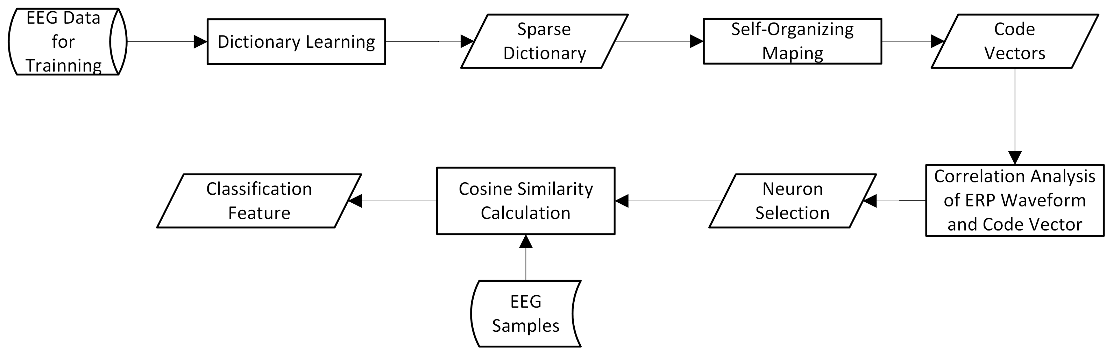
2.4. Feature Extraction Based on Sparse Dictionary Atoms

After obtaining the sparse dictionary, the next step of the proposed method is to perform self-organizing mapping analysis on dictionary atoms, then extract features based on the SOM results. The purpose of using self-organizing mapping analysis is to find the relationship between dictionary atoms and group similar atoms together, so that the waveforms with electrophysiological or cognitive meaning scattered in the over-complete dictionary will be recombined into the network in the code vector of the neuron. Finally, we calculate the cosine similarity between the sample to be recognized and code vectors as classification features.

The feature extraction method can be summarized into three procedures, listed as follows:

• Self-organizing mapping of dictionary atoms;
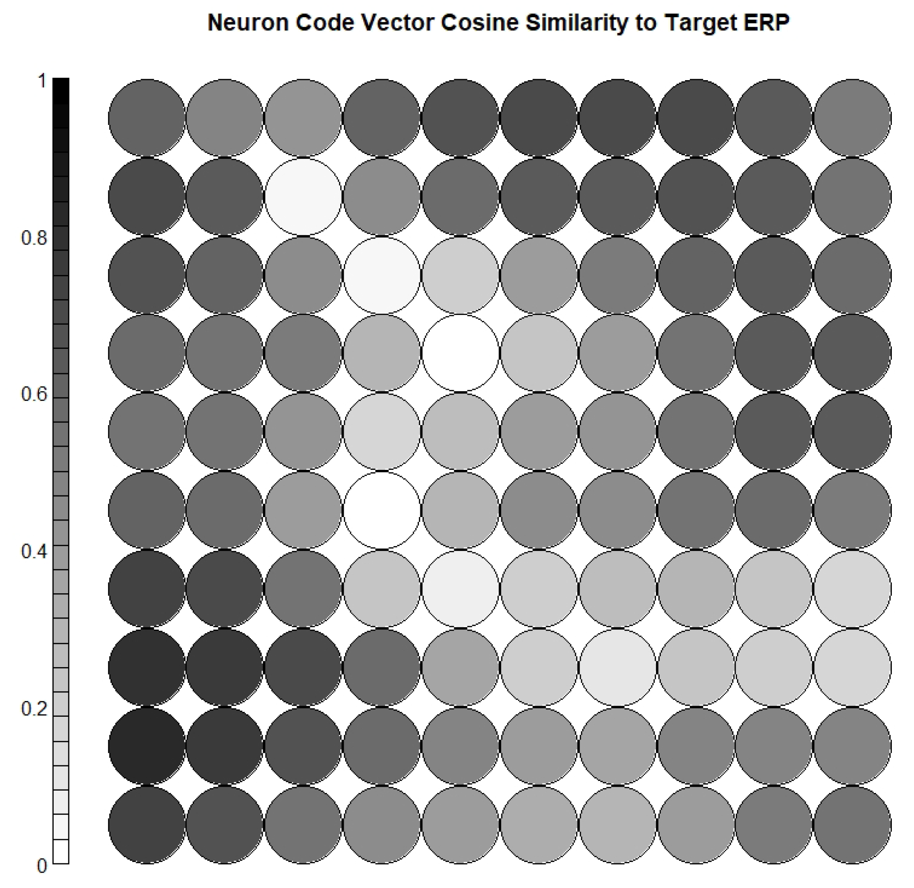
• Calculating the cosine similarity between the weight vector of each neuron and the target ERP waveform, and selecting the most relevant neurons;
• Calculating the cosine similarity between each sample and the selected neuron code vectors as a classification feature.

This method is illustrated in Figure 2.

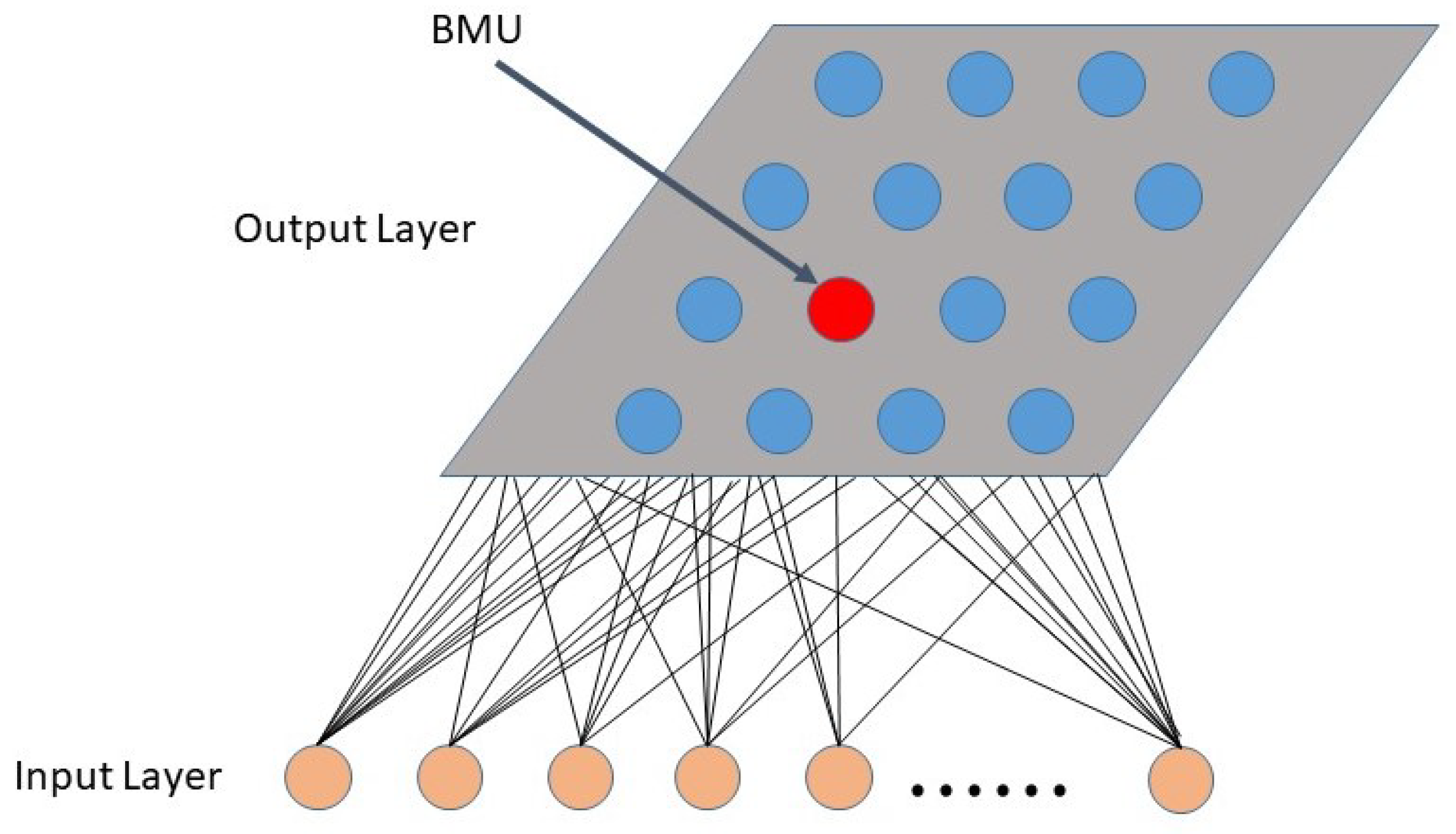
2.4.1. Dictionary Atom Self Organizing Mapping

In this step, we used the dictionary atoms as the SOM network input. When the waveform of a dictionary atom is sent to the network as input, a node in the output layer gets the maximum stimulation and wins, and the nodes around the winning node are also stimulated due to lateral effects. At this time, the network performs a learning operation, and the connection weight vector of the winning node and surrounding nodes is corrected in the direction of the waveform of the input atom. When the input changes, the winning node on the two-dimensional plane is also transferred from the original node to other nodes. In this way, the network uses the entire sparse dictionary to adjust its connection weights in a self-organizing manner and finally enables the network output layer to reflect the distribution of dictionary atoms. The connection weights, that is, the codebook of the entire network, will be a summarization of the entire dictionary. A typical SOM network structure is shown in Figure 3.

Network structure design: The SOM network has two layers, the input layer and the output layer. The length of the input layer is consistent with the length of the dictionary atom. In the output layer, the neurons are distributed in a 2D plane. We chose a square grid topology to arrange the neurons in the output layer. The number of neurons was selected according to the length of the dictionary. Here we chose the number $5\sqrt{N}$, where N is the number of dictionary atoms.

Network initialization: This method uses random data to initialize the the weight of the output layer. Although the use of linear initialization and other methods can achieve faster learning speed, in the scope of the proposed method, speed is not a major concern element. Since there may be a potential linear relationship between the dictionary atoms obtained by K-SVD, if linear initialization is used, the training result of the network will be affected. Random initialization can prevent the linear relationship between dictionary atoms from affecting the learning results of the network.

SOM learning method: We chose the online sequential-learning method for SOM learning, rather than the batch-learning algorithm. Although the number of dictionary atoms is determined, batch-learning seems to be a better choice. However, batch-learning has the following shortcomings [32]: 1. The arrangement of neurons is not as good as sequential learning algorithms. In the application of this article, we hope that the network can bring similar neurons closer in spatial distribution. 2. It is more sensitive to the selection of the initial value, and as mentioned above, we choose a random value as the initial value, and the uncertainty of the result of the combined learning increases. Therefore, in the scope of this article, the sequential-learning method that imitates online training is a better choice.

The process of dictionary atoms SOM analysis is as follows:

• Set the weight of each neuron to a random initial value; set a larger initial neighborhood, and set the number of cycles of the network t, set the number of neurons in the network to M;
• Input a dictionary atom Dk into the network $D_k$: $D_k=\{D_{1k},D_{2k},\dots ,D_{nk}\}$, input into the network; n is the length of the dictionary atom;
• Calculate the weight of $D_k$ and all output neurons, which is the Euclidean distance $d_{jk}$ between the code vector, and select the neuron c with the smallest distance from $D_k$, that is, $x_k-W_c=argmin\left(j\right)\left(d_{ij}\right)$, then c is the Winning neuron;
• Update the connection weight of node c and its domain node $w_{ij}\left(t+1\right)=w_{ij}\left(t\right)+\eta \left(t\right)\left(x_i-w_{ij}\left(t\right)\right)$ Among them, $0<\eta \left(t\right)<1$ is the learning rate, which gradually decreases with time;
• Select another dictionary atom to provide the input layer of the network, and return to step 3 until all the dictionary atoms are provided to the network;
• Let $t=t+l$, return to step (2), until $t=T$. In the learning of self-organizing mapping model, usually $500\le T\le$ 10,000. $N_c$ is the neighbor function, which gradually decreases with the increase in the number of learning. $\eta \left(t\right)$ is the learning rate of the network. Since the learning rate $\eta \left(t\right)$ gradually tends towards zero with the increase in time, it is guaranteed that the learning process must be convergent.

2.4.2. Neuron Selection and Feature Extraction

In this step, we need to find the neuron corresponding to the atom with electrophysiological meaning. Here, we use the cosine similarity between the code vector of the neuron and the target ERP waveform to represent the electrophysiological meaning.

After the network training is completed, each dictionary atom is mapped to the neuron in the SOM network. At this time, the code vector of each neuron can represent the average waveform of a class of dictionary atoms mapped to this neuron. Next, calculate the cosine similarity between the code vector of each neuron and the target ERP waveform, and find the neurons closest to the target ERP waveform. Here, the physical meaning of cosine similarity is the similarity between the waveform of the EEG signal sample to be recognized and the code vector of the neuron in the network. The higher the similarity, the more obvious the electrophysiological meaning contained in the code vector, and the more suitable it is for feature extraction. In this article, the definition of cosine similarity is listed in (5).

$$cos\left(\theta \right)=\frac{\mathrm{ERP}·\mathrm{W}}{\left|\mathrm{ERP}\right|\left|\mathrm{W}\right|}=\frac{{\sum }_{i=1}^n{\mathrm{ERP}}_{\mathrm{i}}{\mathrm{W}}_{\mathrm{i}}}{\sqrt{{\sum }_{\mathrm{i}=1}^{\mathrm{n}}{\mathrm{ERP}}_{\mathrm{i}}^2}\sqrt{{\sum }_{\mathrm{i}=1}^{\mathrm{n}}{\mathrm{W}}_{\mathrm{i}}^2}}$$

(5)

In (5), $\mathrm{ERP}$ is the target ERP waveform vector, n is the vector length, and W is the code vector of the neuron.

For the EEG sample to be recognized, the cosine similarity between the sample to be recognized and the code vector of the selected M neurons is calculated, and the classification feature is constructed according to the cosine similarity. The the feature is calculated by Equation (6)

$$\begin{array}{c}\mathrm{feature}\left(y_i\right)=\left[{cos}_1\left(\theta \right),{cos}_2\left(\theta \right),\cdots {cos}_M\left(\theta \right)\right]\hfill \\ {cos}_m\left(\theta \right)=\frac{{\sum }_{j=1}^n{y}_{ij}{W}_{mj}}{\sqrt{{\sum }_{j=1}^n{y}_{ij}^2}\sqrt{{\sum }_{j=1}^n{W}_{mj}^2}}\hfill \end{array}$$

(6)

In (6), $y_i$ is the i-th EEG sample, n is the sample length, and m is the m-th neuron.

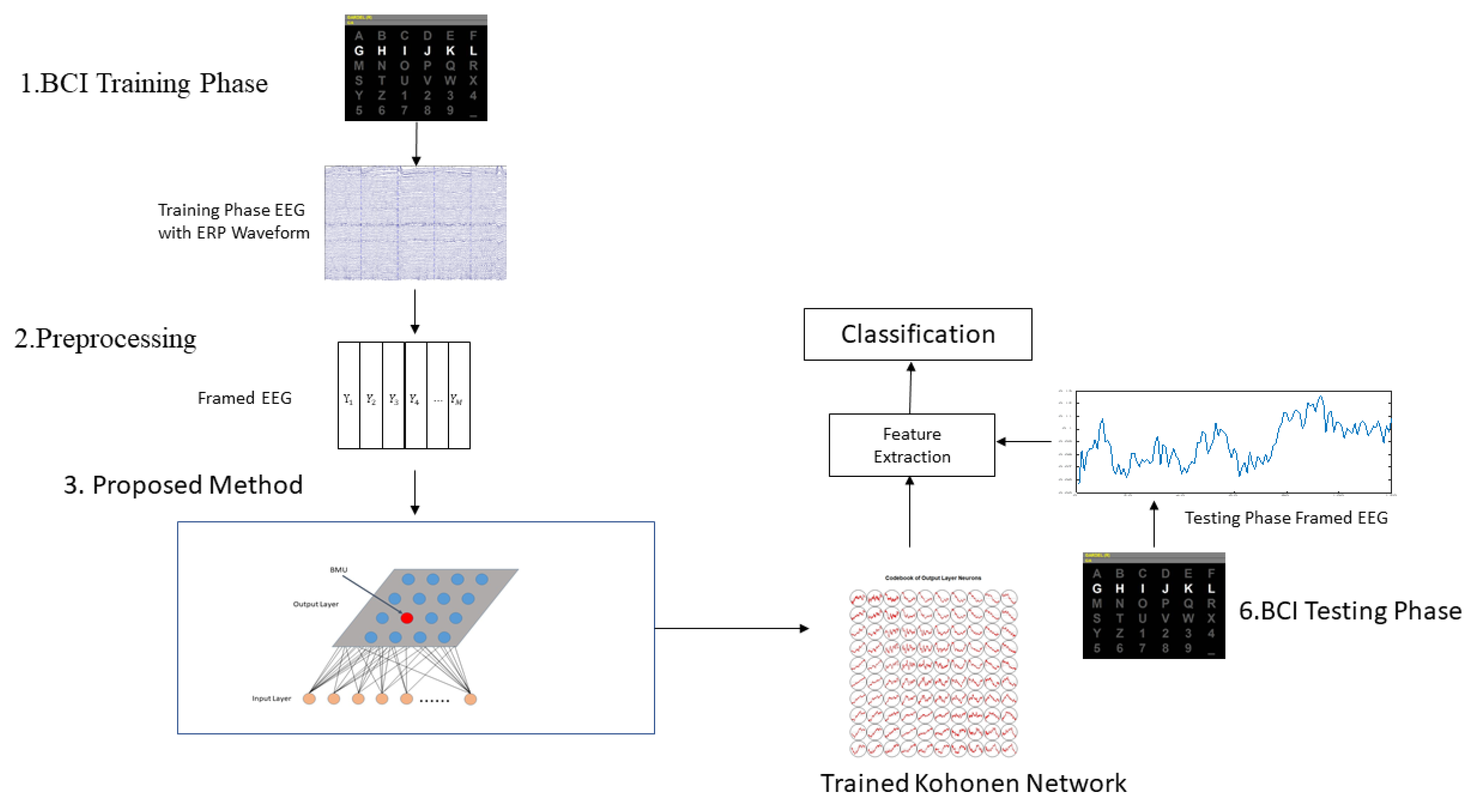
2.5. Application Procedures of Proposed Method in BCI

To apply the proposed method to real-world BCI, the procedures shown in Figure 4 must be followed.

First, obtain a sparse dictionary based on the training samples, and then use the SOM network to perform self-organizing mapping analysis on the sparse dictionary, extract the classification features of the training samples, and train the classifier. For the test samples, follow the same preprocessing method as the training samples, and then use the Kohonen net and classifier parameters obtained from the training samples for feature extraction and classification.

3. Results

3.1. Dataset Description

In this work, we selected a public EEG dataset as the experiment material. This dataset records the EEG data collected from an auditory-event-related potential based speller. The dataset was published by the Berlin University of Technology in 2010 [33]. The experiment data were composed of several trials, each trial included nine sound stimuli, and the interval between each stimulus was 120 ms. The experiment data contained two kinds of stimuli: target and nontarget stimuli. The ratio of the stimuli was 1:8.

EEG signals were recorded monopolarly from 63 wet Ag/AgCl electrodes placed according to the International 10–20 system [33]. EEG signals were amplified using two 32-channel amplifiers (Brain Products) and filtered by an analog bandpass filter between 0.1 and 250 Hz. All channels were referenced to the nose. The sample rate was 1 kHz. Epochs were marked as artifact-contaminated if their peak-to-peak voltage difference in any channel exceeded 100 $\mathsf{\mu }$V. Those epochs were rejected for further analysis.

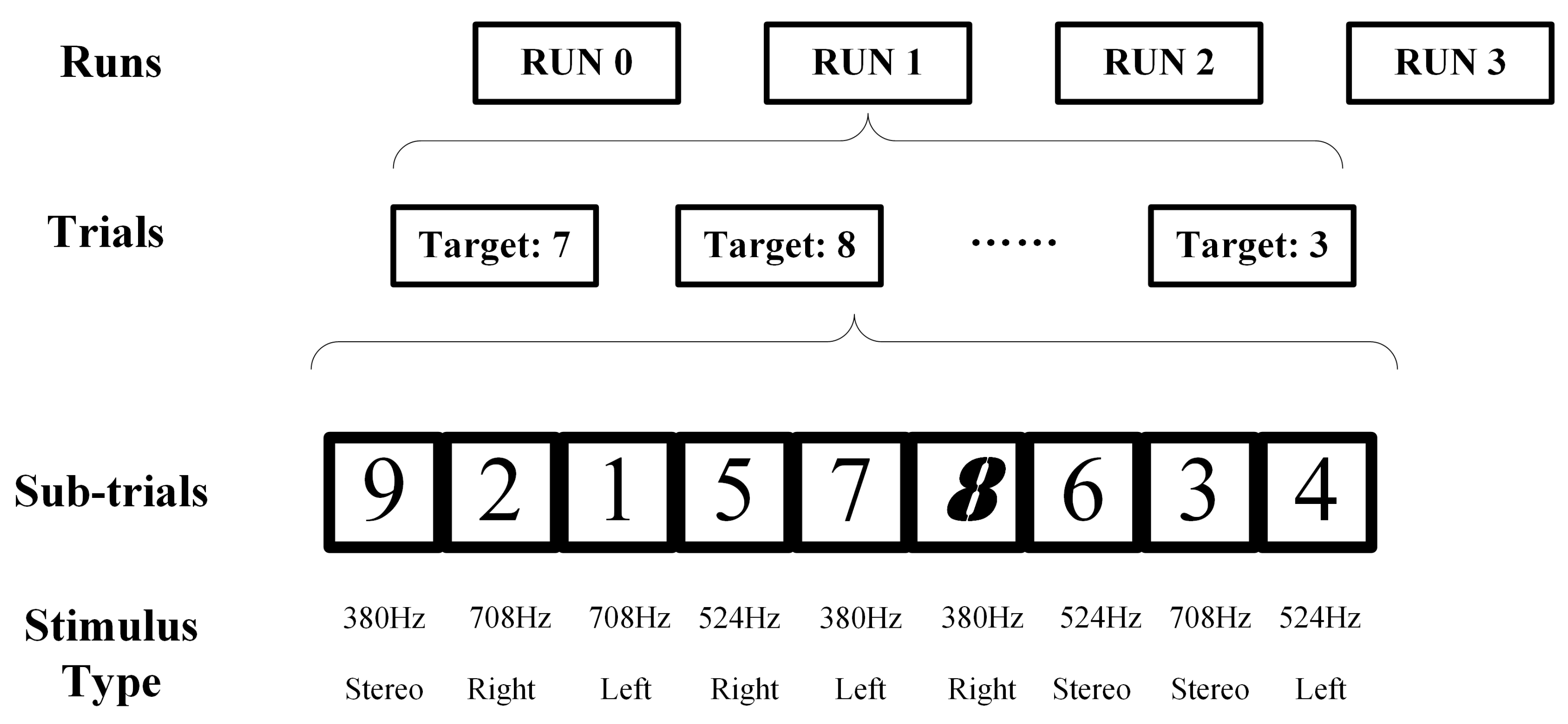
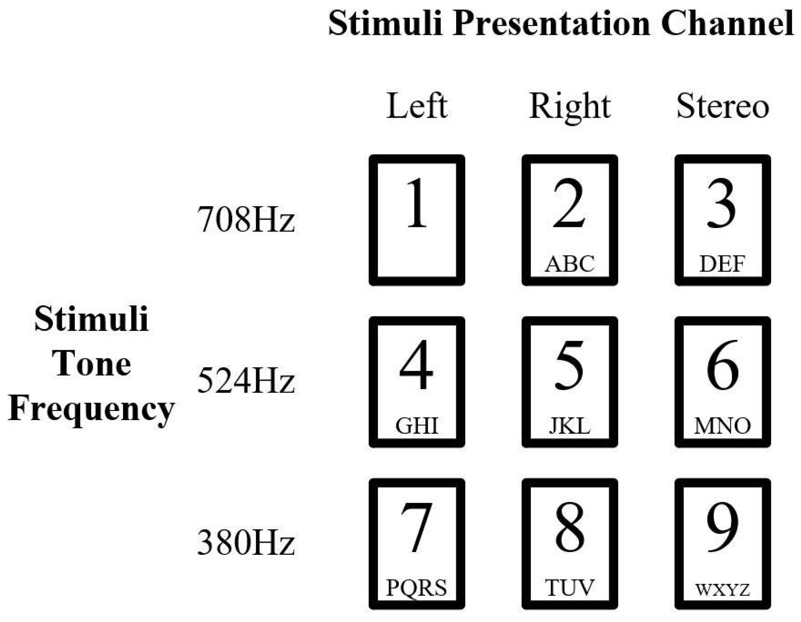
3.1.1. Auditory Stimuli in Experiment Dataset

The audio stimuli in this experiment are artificially generated, single-frequency audio with frequencies of 708 Hz (high), 524 Hz (medium) and 380 Hz (low). Each stimuli is played on the headset in three different channels: on the left channel only, on the right channel only, and on both channels. This constitutes a 3 by 3 combination. Figure 5 shows the design of audio stimuli. This two-dimensional $3\times 3$ design is very similar to the numeric keypad of a classical mobile phone before smartphone era. Each stimulus lasted 100 milliseconds, and the SOA was 225 milliseconds. The stimulus playback sequence is a pseudo-random stimulus sequence so that the subsequent two stimuli do not have the same audio frequency. In addition, the same stimulus is repeated only after at least the other three have appeared.

3.1.2. Experiment Paradigm Design in Dataset

Each subject took part in three calibration runs. In this paper, we used the calibration-run data to train and test the ability of proposed method for target and non-target sub-trials classification. Each calibration runs contained nine trials, and each of the nine types of sound was used as the target stimulus in one run, as shown in Figure 6. In addition, an exercise run without EEG data recording (run 0) was initially performed. Before the start of each trial, the current target number was presented to the subject three times, and the corresponding number on the $3\times 3$ grid was highlighted on the screen.

In the calibration phase, each test consists of 13 or 14 pseudo-random sequences of all nine auditory stimuli. No visual stimulation was given in these tests. When using the last 12 sequences to train the classifier, ignore the first or two sequences to ensure a balanced distribution of stimuli in the calibration data. A representation of a tonal stimulus and corresponding EEG data (time interval up to 800 milliseconds after the stimulus) is called a sub-trial. Therefore, a single experiment provides $9\times 12$ trial epochs (12 target trial epochs and $8\times 12$ non-target trial epochs) for classifier training. The combined training data for all runs include $108\times 27=2916$ trials per subject.

The subjects listened to a sequence of audio stimuli in different combination of tone and channel. One of the nine combinations would be the target. When the subject listened to the target stimulus, the EEG data recorded in this phase would be used to train the BCI classification system to detect the target ERP waveform. When the BCI system detected target ERP waveform from EEG signal, it would virtually trigger a press on the keypad in Figure 5, like typing a text message on traditional mobile phones, before the smartphone era. In the testing phase, the task would change to actually input a sentence. The subject would imagine the keypad key they want to press. Therefore, when a subject was presented the stimulus representing the target key, among other eight no-target stimuli, the trained system would detect the target waveform in EEG data and virtually press the target key. Like a real mobile phone, to type a word would require multiple presses on a keypad, so the trial would repeat multiple times as well.

3.2. Parameter Selection

We divided the continous EEG into frames according to the experimental design of the dataset. We took the time of occurrence of each sound-stimulation event as the starting point of the frames, and selected the next 800 ms as the frame length. At a sampling rate of 150 Hz, each frame contained 120 datapoints.

In this article, we used only one EEG data channel, Cz. The reason for this selection was that the ERP of this electrode was the most obvious in the article of the selected dataset. This article selected the training and testing phase data of the subjects VPnw in the dataset for the sparse performance experiment, and all other subjects except VPnv and VPmg for the classification experiment. Figure 7 shows the averaged target ERP on Cz.

For this specific dataset, the parameters of the proposed method are listed in

Table 1. Parameters in Feature Extraction.

Parameter	Value
K-SVD Sparsity	10
Number of Atoms in Dictionary	512
Atom Length	120
EEGFrame Length	120
EEG Sample Rate	150 Hz
Number of SOM Neurons	100
SOM Topology	$10\times 10$, Square Topology

.

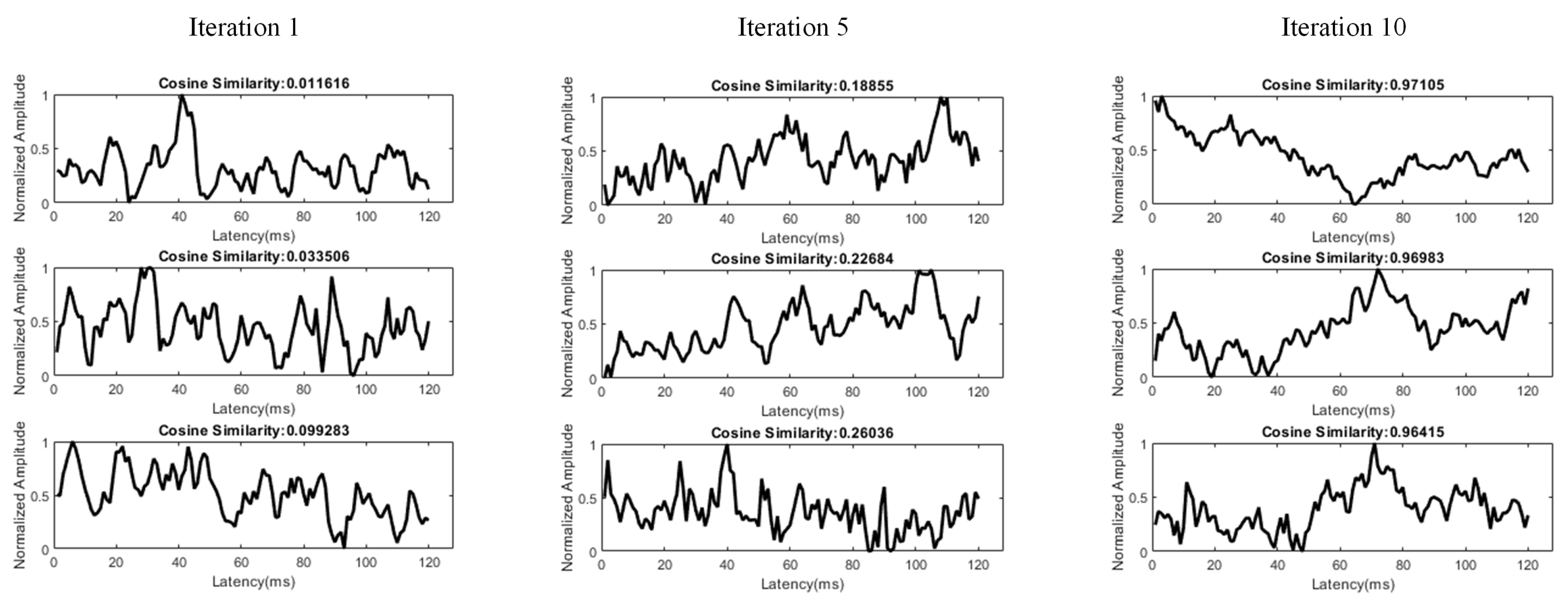
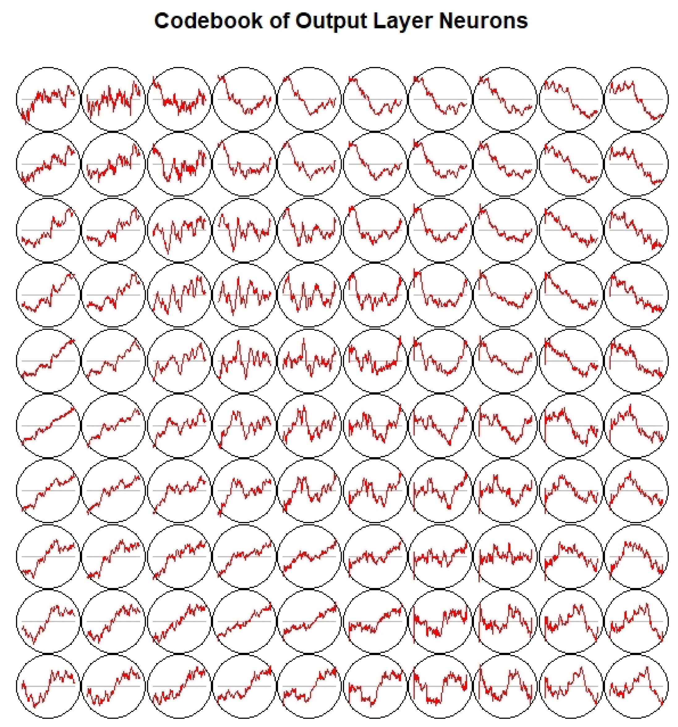
3.3. Dictionary Atom SOM Results

Figure 8 shows the number of hits each neuron won when the dictionary atom was mapped to the trained SOM network. Most of the atoms were concentrated on five neurons, and the distribution of neurons with similar winning times on the network is also closer.

The trained SOM network also placed neurons with similar code vectors nearby, as illustrated in Figure 9. Thanks to SOM, similar dictionary atoms were gathered into the code vectors of neurons, and the positions of neurons corresponding to similar code vectors on the network were placed adjacent to each other.

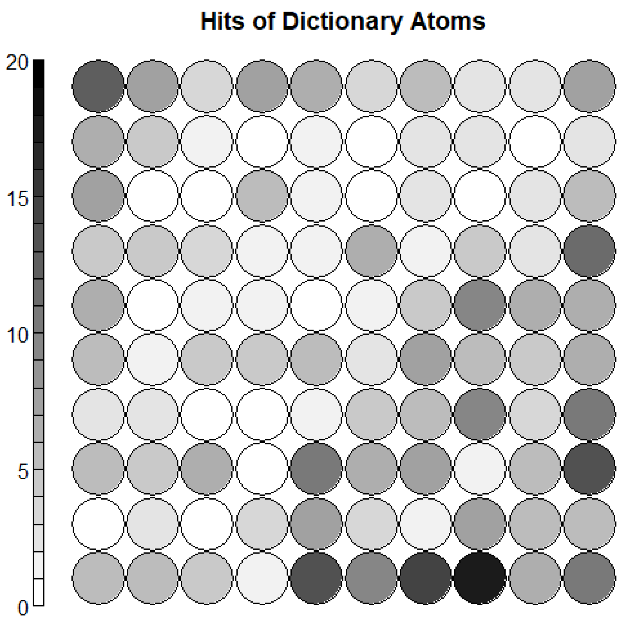
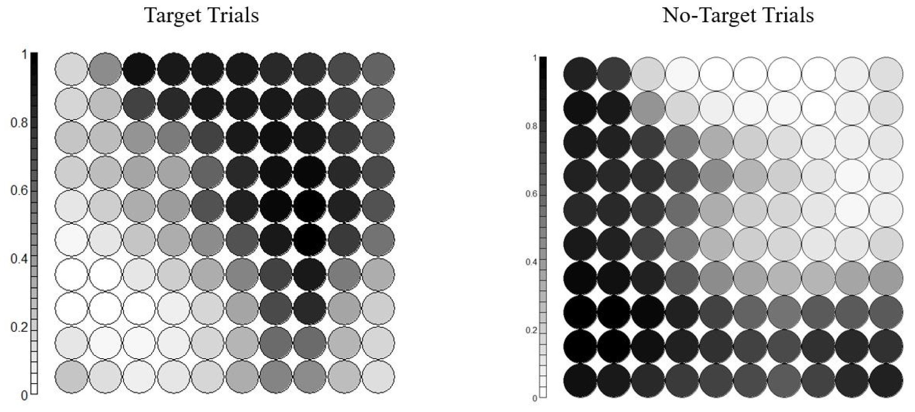
3.4. Neuron Selection and Feature Extraction Results

Figure 10 illustrated the cosine similarity value between the code vector of the neuron and the target ERP waveform obtained after superimposing and averaging. All values were projected to ($0,1$). The code vectors of some neurons had a high correlation with the target ERP. The result showed that the electrophysiological meaning of atoms was aggregated into the codebook of the SOM network.

For different types of EEG sample, the cosine similarity between the samples and the code vectors differs. Figure 11 showed the averaged abstract values of cosine similarity between the EEG data samples and the neuron code vectors. The data are projected to the range $\left[0,1\right]$ for display. It can be seen that for two types of EEG sample, the distribution of the cosine similarity values was significantly different, which proves that the cosine similarity value between the sample and the code vector can be used as a classification feature.

3.5. Classification Stage and Result Analysis

3.5.1. Classification Stage Design

We selected the training phase data of the subjects in the dataset for experiments. There are two classification classes: EEG data frame from target subtrials and EEG data frame from non-target sub-trials. Subject VPnw and subject Vpmg are excluded, which is consistent with the analysis of the original data set. In this paper, we only used one EEG data channel from Cz. The reason for this selection is that the ERP waveform is most obvious [33] in Cz. In this article, we used SVM to construct a classifier. The classification feature is the cosine similarity between the sample to be recognized and the code vector of the selected six neurons. Select the EEG samples of the subjects in the training phase and divide them into five parts for cross-validation: one is used for testing and four parts are used for training the sparse dictionary, SOM network and classifier. To balance the classes, we used classwise balanced accuracy, which is the average decision accuracy across classes (target vs. non-target).

3.5.2. Classification Result

Using the method described in this article, we obtained an average class-wise balanced accuracy of 76.4% for all nine subjects, as shown in

Table 2. Binary Classification Accuracy Comparision.

Method	Subjects
	VPnv	VPny	VPnz	VPoa	VPob	VPoc	VPod	VPja	VPoe	Avg
Proposed	78.00%	75.90%	75.10%	73.60%	79%	79.50%	71.20%	81.00%	74.50%	76.42%
Original	77.0%	75.0%	74.4%	72.2%	78.6%	79.6%	70.0%	82.0%	73.2%	75.78%

. Compared with the 75.8% accuracy reported in original paper, proposed method used only one channel of data and still obtained a similar result to the benchmark method using 64 channels of data for classification. We ran the whole classification experiment on a persoanl computer with Intel i5-4690 CPU and 16 GB RAM. The mean classification computation time for each subject was 20.2 s, including feature extraction and classification for 2915 samples.

3.5.3. Review and Comparison of Classification Result

Compared with studies based on other similar BCI experiments, the classification accuracy obtained by proposed method matches state-of-art methods, with advantages in the data amount used for training and required preprocessing procedures, as shown in

Table 3. State-of-art Study Comparision.

Category	Study	Accuracy	Data Amount Used	Preprocessing Procedures and Computation Required
Visual ERP	Saavedra et al. [35]	75%	Moderate (Multiple Channels)	Moderate for ERP research
	Bostanov [34]	77%	Moderate (Multiple Channels)	Moderate for ERP research
	Kabbara1 et al. [36]	80%	Moderate (Multiple Channels)	Moderate for ERP research
Auditory ERP	Ogino et al. [37]	79%	Moderate (Multiple Channels)	Moderate for ERP research
	Proposed Method	76.2%	Minimum (Single Channel)	Only simple procedures minimum computation
	Höhne et al. [33]	75.6%	Moderate (Multiple Channels)	Moderate for ERP research
Deep Learning	Kundu et al. [38]	90.5%	Large (Multi Channel) (Large Group of Subjects)	Only simple procedures. Huge computation effort.
	Lee et al. [39]	93%	Large (Multi Channel) (Large Group of Subjects)	Only simple procedures. Huge computation effort.

.

In the BCI Competition IIb dataset published in 2003, Bostanov used Continous Wavelet Transformation (CWT) for feature extraction and obtained 77% accuracy of binary classification [34]. In a similar brain-computer interface study of visual P300 ERP waveforms, Saavedra et al. proposed Wavelet-Based Semblance Methods to Enhance the Single-Trial ERP detection, and reported 75% classification accuracy [35]. Kabbara1 et al. proposed brain network connection as a classification feature; the accuracy rate obtained was about 80% [36]. Compared with these methods, the accuracy obtained by the proposed method is close to these methods, while they generally used ten or more channels. In these experimental paradigms of the visual P300 brain-computer interface, due to the long interval between visual stimuli, there is no overlap of ERP waveforms in the dataset used in this study, which had a negative impact on performance.

In the auditory ERP brain-computer interface research, Mikito Oino et al. used single-channel EEG data and the traditional Step-Wise Linear Discriminant Analysis(SWLDA) method to obtain 79% accuracy [37]. Fazel-Rezai et al. conducted in-depth analysis and believed that it is difficult to improve the accuracy of binary classifications in the auditory brain-computer interface [40]. Therefore, the significance of the proposed method lies in the fact that fewer data are needed for classification, which is very important in wearable brain-computer interface devices. When comparing with other methods, it should be noted that, in addition to accuracy, the proposed method does not require common preprocessing operations such as artifact removal and filtering. It only requires down-sampling and normalization operations. Compared with other methods, it reduces computation effort, since artifact rejection is often time-consuming and requires heavy computation. The main reason for this is that the KSVD modeling process will put the artifact interference into separate dictionary atoms.

In addition to traditional feature extraction and classification methods, deep learning methods, especially the convolutional neural network (CNN) [41], have already been applied to BCI applications. Kundu et al. introduced CNN to Visual ERP BCI and achieved higher accuracy [38]. Then, Lee found that with a large dataset, CNN can provide a comparable performance in P300 ERP-based BCI with zero training [39]. Compared with the method in this paper, a higher amount of data is still needed for training in the CNN-based method. Besides, Zhang et al. proposed that the deep-learning method has obvious vulnerabilities and can be attacked by adversarial examples [42]. This makes deep-learning methods unstable in practical applications.

To summary, compared to common methods, the proposed method obtained comparable classification results, with a smaller amount of data and calculation required.

4. Discussion

The current mainstream EEG feature extraction methods for ERP-based BCI usually require multi-channel data and have difficulties in processing non-stationary waveform. Sparse modelling-based methods provide certain improvements, but the sparse features are often unstable and challenging to interpret. Therefore, there is the question of how to extract better features to overcome those drawbacks. In order to answer this question, we proposed a novel EEG signal feature extraction method for event-related potential recognition. In this method, we first performed sparse dictionary-learning on the EEG signals of the training set to obtain the sparse dictionary, and then performed self-organize mapping on the dictionary atoms, and used the cosine similarity between the sample to be recognized and the code vectors of the SOM network as the classification feature.

The results in Figure 9 and Figure 10 showed that the code vectors in the SOM network trained by sparse dictionary atoms were highly similar to the ERP waveforms obtained by multiple superpositions. This means that the proposed method successfully processed non-stationary ERP waveform. As shown in Table 2, the proposed method could provide stable and useful classification features from single-channel data. The results proved that the proposed method is the answer to the question above. The classification result was comparable to other studies, as presented in Table 3. Compared with traditional and most state-of-art ERP extraction methods, this method achieved a similar classification accuracy result with fewer data required for it to work and less computation effort.

This method has three strengths. First, based on the results in Figure 9 and Figure 10, the features extracted by the method in this article use sparse dictionary atoms as a bridge to establish a connection between the EEG frames to be recognized and the target ERP waveform. This gives the extracted features a certain electrophysiological meaning. Second, proposed method only requires single-channel data, and ERP can be extracted in a single trial. Third, this method requires fewer preprocessing steps than traditional methods, especially as the artifact rejection is not required in the proposed method.

Based on the above strengths, the proposed method is most suitable for wearable brain-computer interface applications. In this application scenario, the energy efficiency of data transmission is low, and the data analysis and computation capabilities of the device itself are limited, so the data must be transmitted to the remote server for complex analysis. When using the method in this paper, since the SOM network has been trained, only a few cosine distances need to be calculated locally to perform classification. On the other hand, when the remote server and the wearable brain-computer interface device share a sparse dictionary, only sparse data need to be transmitted to recover the collected EEG waveforms on the remote server for further and more complex analysis tasks.

The proposed methods have limitations and can be further improved on in the future, mainly in the following aspects: First, in the proposed method, the Best Matching Unit (BMU) is selected by Euclidean distance. Other distance measurements may provide better results. Second, the cosine similarity in this article is used as a classification feature. If we use other calculation methods to determine the time series relationship, we may get features more adaptive to the nature of the samples.

In summary, in this article, we proposed an EEG feature-extraction method for BCI applications. The classification results on the public dataset show that this method requires fewer preprocessing steps and a smaller amount of data than traditional methods and other state-of-art studies. The features obtained by the proposed method were more readable. The above strengths give this method advantages in wearable brain-computer interface applications.

5. Conclusions

The sparse dictionary atoms contain the scattered information of samples. Our proposed method showed that SOM can effectively aggregate the scattered waveforms of ERP in dictionary atoms and be used to extract classification features. The test results on a public dataset showed that the features obtained by the proposed method in this article have better electrophysiological meaning, and only one channel of data is needed to achieve a comparable binary classification accuracy to the baseline method. Therefore, the proposed method achieved the goal of extracting features with electrophysiological meaning and use a smaller amount of data. In future work, we will continue to explore possible variants of SOM to fully exploit the sparse dictionary for feature extraction.

References

1. James, C.J.; Lowe, D. Extracting multisource brain activity from a single electromagnetic channel. Artif. Intell. Med. 2003, 28, 89–104. [Google Scholar] [CrossRef]
2. Hu, L.; Mouraux, A.; Hu, Y.; Iannetti, G.D. A novel approach for enhancing the signal-to-noise ratio and detecting automatically event-related potentials (ERPs) in single trials. Neuroimage 2010, 50, 99–111. [Google Scholar] [CrossRef]
3. Azlan, W.A.W.; Low, Y.F. Feature extraction of electroencephalogram (EEG) signal—A review. In Proceedings of the 2014 IEEE Conference on Biomedical Engineering and Sciences (IECBES), Sarawak, Malaysia, 8–10 December 2014; pp. 801–806. [Google Scholar]
4. Farwell, L.; Donchin, E. Talking off the top of your head: Toward a mental prosthesis utilizing event-related brain potentials. Electroencephalogr. Clin. Neurophysiol. 1988, 70, 510–523. [Google Scholar] [CrossRef]
5. Jung, T.; Makeig, S.; Westerfield, M.; Townsend, J.; Courchesne, E.; Sejnowski, T. Independent component analysis of single-trial event-related potentials. In Proceedings of the International workshop on Independent component analysis and blind signal separation, Aussois, France, 11–15 January 1999; pp. 173–179. [Google Scholar]
6. Huang, N.E.; Wu, Z. A review on Hilbert-Huang transform: Method and its applications to geophysical studies. Rev. Geophys. 2008, 46. [Google Scholar] [CrossRef] [Green Version]
7. Gao, C.; Ma, L.; Li, H. An ICA/HHT Hybrid Approach for Automatic Ocular Artifact Correction. Int. J. Pattern Recognit. Artif. Intell. 2015, 29, 1558001. [Google Scholar] [CrossRef]
8. Lee, W.L.; Tan, T.; Falkmer, T.; Leung, Y.H. Single-trial event-related potential extraction through one-unit ICA-with-reference. J. Neural Eng. 2016, 13, 066010. [Google Scholar] [CrossRef] [PubMed]
9. Eilbeigi, E.; Setarehdan, S.K. Detecting intention to execute the next movement while performing current movement from EEG using global optimal constrained ICA. Comput. Biol. Med. 2018, 99, 63–75. [Google Scholar] [CrossRef]
10. Zhang, J.; Bi, L.; Lian, J.; Guan, C. A Single-Trial Event-Related Potential Estimation Based on Independent Component Analysis and Kalman Smoother. In Proceedings of the 2018 IEEE/ASME International Conference on Advanced Intelligent Mechatronics (AIM), Auckland, New Zealand, 9–12 July 2018; IEEE: Piscataway, NY, USA, 2018; pp. 7–12. [Google Scholar] [CrossRef]
11. Fukami, T.; Watanabe, J.; Ishikawa, F. Robust estimation of event-related potentials via particle filter. Comput. Methods Programs Biomed. 2016, 125, 26–36. [Google Scholar] [CrossRef]
12. Ting, C.M.; Salleh, S.H.; Zainuddin, Z.M.; Bahar, A. Modeling and estimation of single-trial event-related potentials using partially observed diffusion processes. Digit. Signal Process. Rev. J. 2015, 36, 128–143. [Google Scholar] [CrossRef]
13. Delaney-Busch, N.; Morgan, E.; Lau, E.; Kuperberg, G.R. Neural evidence for Bayesian trial-by-trial adaptation on the N400 during semantic priming. Cognition 2019, 187, 10–20. [Google Scholar] [CrossRef]
14. Zeyl, T.; Yin, E.; Keightley, M.; Chau, T. Adding real-time Bayesian ranks to error-related potential scores improves error detection and auto-correction in a P300 speller. IEEE Trans. Neural Syst. Rehabil. Eng. 2016, 24, 46–56. [Google Scholar] [CrossRef] [PubMed]
15. Wen, D.; Jia, P.; Lian, Q.; Zhou, Y.; Lu, C. Review of sparse representation-based classification methods on EEG signal processing for epilepsy detection, brain-computer interface and cognitive impairment. Front. Aging Neurosci. 2016, 8, 172. [Google Scholar] [CrossRef] [PubMed]
16. Dai, Y.; Wang, X.; Li, X.; Tan, Y. Sparse EEG compressive sensing for web-enabled person identification. Meas. J. Int. Meas. Confed. 2015, 74, 11–20. [Google Scholar] [CrossRef]
17. Wu, Q.; Zhang, Y.; Liu, J.; Sun, J.; Cichocki, A.; Gao, F. Regularized Group Sparse Discriminant Analysis for P300-Based Brain-Computer Interface. Int. J. Neural Syst. 2019, 29. [Google Scholar] [CrossRef] [PubMed]
18. Mo, H.; Luo, C.; Jan, G.E. EEG classification based on sparse representation. In Proceedings of the International Joint Conference on Neural Networks, Anchorage, AK, USA, 14–19 May 2017; IEEE: Piscataway, NY, USA, 2017; Volume 2017, pp. 59–62. [Google Scholar] [CrossRef]
19. Shin, Y.; Lee, S.; Ahn, M.; Cho, H.; Jun, S.C.; Lee, H.N. Simple adaptive sparse representation based classification schemes for EEG based brain-computer interface applications. Comput. Biol. Med. 2015, 66, 29–38. [Google Scholar] [CrossRef]
20. Yuan, S.; Zhou, W.; Yuan, Q.; Li, X.; Wu, Q.; Zhao, X.; Wang, J. Kernel Collaborative Representation- Based Automatic Seizure Detection in Intracranial EEG. Int. J. Neural Syst. 2015, 25, 1550003. [Google Scholar] [CrossRef]
21. Yu, H.; Lu, H.; Ouyang, T.; Liu, H.; Lu, B.L. Vigilance detection based on sparse representation of EEG. In Proceedings of the 2010 Annual International Conference of the IEEE Engineering in Medicine and Biology, Buenos Aires, Argentina, 31 August–4 September 2010; pp. 2439–2442. [Google Scholar] [CrossRef]
22. Shin, Y.; Lee, H.N.; Balasingham, I. Fast L1-based sparse representation of EEG for motor imagery signal classification. In Proceedings of the 2016 38th Annual International Conference of the IEEE Engineering in Medicine and Biology Society (EMBC), Orlando, FL, USA, 16–20 August 2016; IEEE: Piscataway, NY, USA, 2016; Volume 2016, pp. 223–226. [Google Scholar] [CrossRef]
23. Ayesha, S.; Hanif, M.K.; Talib, R. Overview and comparative study of dimensionality reduction techniques for high dimensional data. Inf. Fusion 2020, 59, 44–58. [Google Scholar] [CrossRef]
24. Kohonen, T. Self-organized formation of topologically correct feature maps. Biol. Cybern. 1982, 43, 59–69. [Google Scholar] [CrossRef]
25. Ngan, S.C.; Yacoub, E.S.; Auffermann, W.F.; Hu, X. Node merging in Kohonen’s self-organizing mapping of fMRI data. Artif. Intell. Med. 2002, 25, 19–33. [Google Scholar] [CrossRef]
26. Liao, W.; Chen, H.; Yang, Q.; Lei, X. Analysis of fMRI data using improved self-organizing mapping and spatio-temporal metric hierarchical clustering. IEEE Trans. Med. Imaging 2008, 27, 1472–1483. [Google Scholar] [CrossRef]
27. Kurth, C.; Gilliam, F.; Steinhoff, B. EEG spike detection with a Kohonen feature map. Ann. Biomed. Eng. 2000, 28, 1362–1369. [Google Scholar] [CrossRef] [PubMed]
28. Hemanth, D.J.; Anitha, J.; Son, L.H. Brain signal based human emotion analysis by circular back propagation and Deep Kohonen Neural Networks. Comput. Electr. Eng. 2018, 68, 170–180. [Google Scholar] [CrossRef]
29. Diaz-Sotelo, W.J.; Roman-Gonzalez, A.; Vargas-Cuentas, N.I.; Meneses-Claudio, B.; Zimic, M. EEG Signals Processing Two State Discrimination Using Self-organizing Maps. In Proceedings of the 2018 IEEE International Conference on Automation/XXIII Congress of the Chilean Association of Automatic Control (ICA-ACCA), Concepcion, Chile, 17–19 October 2018; IEEE: Piscataway, NY, USA, 2018; pp. 1–4. [Google Scholar]
30. Hämäläinen, T.D. Parallel Implementation of Self-Organizing Maps. In Self-Organizing Neural Networks: Recent Advances and Applications; Springer: Berlin/Heidelberg, Germany, 2001; pp. 245–278. [Google Scholar]
31. Aharon, M.; Elad, M.; Bruckstein, A. K-SVD: An Algorithm for Designing Overcomplete Dictionaries for Sparse Representation. IEEE Trans. Signal Process. 2016, 54, 4311–4322. [Google Scholar] [CrossRef]
32. Fort, J.C.; Letrémy, P.; Cottrell, M. Advantages and drawbacks of the Batch Kohonen algorithm. In Proceedings of the ESANN 2002, 10th Eurorean Symposium on Artificial Neural Networks, Bruges, Belgium, 24–26 April 2002; pp. 223–230. [Google Scholar]
33. Höhne, J.; Schreuder, M.; Blankertz, B.; Tangermann, M. A Novel 9-Class Auditory ERP Paradigm Driving a Predictive Text Entry System. Front. Neurosci. 2011, 5, 99. [Google Scholar] [CrossRef] [PubMed] [Green Version]
34. Bostanov, V. BCI competition 2003-data sets Ib and IIb: Feature extraction from event-related brain potentials with the continuous wavelet transform and the t-value scalogram. IEEE Trans. Biomed. Eng. 2004, 51, 1057–1061. [Google Scholar] [CrossRef] [PubMed]
35. Saavedra, C.; Salas, R.; Bougrain, L. Wavelet-Based Semblance Methods to Enhance the Single-Trial Detection of Event-Related Potentials for a BCI Spelling System. Comput. Intell. Neurosci. 2019, 2019. [Google Scholar] [CrossRef] [PubMed] [Green Version]
36. Kabbara, A.; Khalil, M.; El-Falou, W.; Eid, H.; Hassan, M. Functional Brain Connectivity as a New Feature for P300 Speller. PLoS ONE 2016, 11, e0146282. [Google Scholar] [CrossRef]
37. Ogino, M.; Kanoga, S.; Muto, M.; Mitsukura, Y. Analysis of Prefrontal Single-Channel EEG Data for Portable Auditory ERP-Based Brain–Computer Interfaces. Front. Hum. Neurosci. 2019, 13, 250. [Google Scholar] [CrossRef]
38. Kundu, S.; Ari, S. Fusion of Convolutional Neural Networks for P300 Based Character Recognition. In Proceedings of the 2019 International Conference on Information Technology (ICIT), Bhubaneswar, India, 19–21 December 2019; IEEE: Piscataway, NY, USA; pp. 155–159. [Google Scholar]
39. Lee, J.; Won, K.; Kwon, M.; Jun, S.C.; Ahn, M. CNN with Large Data Achieves True Zero-Training in Online P300 Brain-Computer Interface. IEEE Access 2020, 8, 74385–74400. [Google Scholar] [CrossRef]
40. Fazel-Rezai, R.; Allison, B.; Guger, C.; Sellers, E.; Kleih, S.; Kübler, A. P300 brain computer interface: Current challenges and emerging trends. Front. Neuroeng. 2012, 5, 14. [Google Scholar] [CrossRef] [Green Version]
41. Lecun, Y.; Bottou, L.; Bengio, Y.; Haffner, P. Gradient-based learning applied to document recognition. Proc. IEEE 1998, 86, 2278–2324. [Google Scholar] [CrossRef] [Green Version]
42. Zhang, X.; Wu, D. On the Vulnerability of CNN Classifiers in EEG-Based BCIs. IEEE Trans. Neural Syst. Rehabil. Eng. 2019, 27, 814–825. [Google Scholar] [CrossRef] [PubMed] [Green Version]
Figure 1. Dictionary atom learning example in K-SVD algorithm after several iterations. The cosine similarity shows the similarity between the atom and the target ERP waveform.
Algorithms 13 00259 g001
Figure 2. Flowchart of Feature Extraction Method.
Algorithms 13 00259 g002
Figure 3. Self-organizing mapping network.
Algorithms 13 00259 g003
Figure 4. Application Procedures of Proposed Method in BCI.
Algorithms 13 00259 g004
Figure 5. The audio stimuli design.
Algorithms 13 00259 g005
Figure 6. The experiment paradigm.
Algorithms 13 00259 g006
Figure 7. Averaged Target ERP.
Algorithms 13 00259 g007
Figure 8. Hits of Dictionary Atoms for SOM neurons.
Algorithms 13 00259 g008
Figure 9. Codebook of SOM network.
Algorithms 13 00259 g009
Figure 10. Cosine similarity between averaged Target ERP and code vectors.
Algorithms 13 00259 g010
Figure 11. Cosine similarity between code vectors and two types of EEG sample.
Algorithms 13 00259 g011