A Solving Algorithm for Nonlinear Bilevel Programing Problems Based on Human Evolutionary Model

Abstract

An algorithm based on the human evolutionary model is proposed for solving nonlinear bilevel programing problems. In view of the hierarchical structure of this problem, the algorithm is designed through feeding back the optimal solution of the lower-level problem to the upper-level. Based on the quality of individuals at each iteration, this proposed algorithm can independently change the population size to achieve the balance between global and local searching ability during the progress of evolution, which can perform an exhaustive search in the whole landscape through creating an individual by using the tabu search method. Finally, we test four typical bilevel programing problems by using the proposed algorithm to verify its feasibility. The experimental results indicate the proposed algorithm can not only solve bilevel programing problems but also get the global optimal solution.

1. Introduction

According to the existing studies on the multi-level programming problem, the mathematical model for this kind of problem can play a vital role in addressing complicated problems involving multiple decision-makers [1,2]. We also find that the notable feature of these problems is of containing more than one decision maker, who has a major conflict due to the limitation of resources. For the bilevel programming problem, the upper and lower decision-makers have different anticipated goals described as the objective functions; resource limitation is shown as constraint conditions and the decision variables. Furthermore, referring to the basic game theory, the decision process of the problem can be essentially characterized as two decision makers with different goals successively making their own decisions in accordance with the leader–follower hierarchical relationship. In other words, the upper maker firstly made the decision, and then the lower decision maker made the decision within the allowable range in the light of the upper level decision results. Therefore, we can conclude that the final results of the upper level decision-maker were not only concerned with the decision variables of the upper level problem but also connected with the optimal solution to the lower level problem, and the lower level decision maker’s optimal solution was affected by the upper level decision variables similarly. In other words, both decisions were affected rather than completely determined by the input of the other.

The bilevel program problem can be used to describe many practical problems, such as engineering design, economic policy, traffic problems, etc. In consequence, many researchers have made an intensive studies on this kind of hierarchical problem, making not only great achievements in theoretical research on the bilevel program problem, but also with proposed abundant algorithms for solving the problem [3,4,5,6,7,8,9].

Nevertheless, the bilevel program problem is a non-convex problem, so it is very difficult for solving the problem [5]. Jeroslow [10] firstly indicated that the bilevel program problem is a non-deterministic polynomial hard problem(NP-hard problem). Subsequently, this conclusion was proven by Ben-Ayed and Blair [11] and Bard [12]. Vicente, Savard, and Judice [13] further pointed out that searching for the local optima to the linear bilevel program problem is also an NP-hard problem. Deng [14] elaborated the complexity of the problem in details.

The algorithms presented in the existing literatures are generally divided into two categories: the traditional approaches and the heuristic algorithms. The former assumes the function is differentiable and continuous and that they are constructed based on the feature and optimality condition of bilevel programming problem(BLPP). The algorithms in this category include K-best algorithm, peak searching method, exact penalty function, descent direction method, complementary pivoting algorithm, equilibrium point algorithm, etc. [8]. Those algorithms commonly depend on the search space of the specific problem. However, some problems cannot satisfy the assumptions, for example BLPP is not differentiable. Therefore, those algorithms restrict in their ability to solve many practical problems because most of them lack the required mathematical properties for these kind of algorithms.

For the second category, there are no limitations on the differentiability of the functions, so many researchers tend to develop heuristic algorithms for solving BLPP, including: the genetic algorithm (GA) [15,16,17,18], the state transition algorithm (STA) [9], particle swarm optimization (PSO) [19,20,21], tabu search (TS) [22], multi-sine cosine algorithm [23], artificial neural network (ANN) [16,24,25,26], homotopy method [27], evolutionary algorithm (EA) [28,29,30], simulated annealing (SA) [17], artificial bee colony algorithm (ABC) [31], ant colony algorithm (AC) [32], etc.

In order to get a better solution faster for BLPP, some scholars began to propose a hybrid intelligent algorithm. For instance, Watada et al. [16] combined a genetic algorithm and a dual recurrent neural network to present a hybrid algorithm, while Yi et al. [17] proposed a hybrid method through integrating the simulated annealing and genetic algorithms. Similarly, backpropagation artificial neural network integrated with particle swarm optimization was also proposed to deal with these problems [24,26]; another novel method was proposed by integrating particle swarm optimization and estimated distribution algorithm [33], etc. Unfortunately, there are plenty of parameters to adjust for both single and hybrid intelligent algorithms. As the same time, there are no common criteria for the approach to adapt the parameters to every specific problem. Although, it is practicable that the proper parameter combination was produced by trial, by itself, the fixed parameter is not fit for the dynamic feature of evolutionary algorithms [34].

The human evolutionary model proposed in Reference [34] is a novel self-adaptive algorithm that adjusts its parameters in accordance with algorithm performance, so we employ this model to construct a solving algorithm for nonlinear BLPP. Based on the decision process of the problems mentioned above, the basic process of this algorithm proposed in this paper is as follows: for the given upper level decision variable, the lower level problem is solved by GA and the corresponding optimal solution is delivered to the upper level, and then the upper level program is solved by the human evolutionary model (HEM). The algorithm instantaneously adjusts the population size in light of its performance to keep the local and goal search ability, and also takes advantage of the tabu search method for generating a new individual to avoid being trapped in a visited region for the sake of accelerating convergence. Therefore, the algorithm can control the searching process and conduct the evolutionary procedure for two level problems so that this proposed algorithm can efficiently overcome the difficulty of the bilevel problem and have a better performance.

This paper is organized as follows: Section 2 introduces the basic definitions and assumptions of BLPP. Section 3 introduces some vital concepts of HEM and proposes the algorithm for solving BLPP. The numerical experiments and results are given in Section 4. Section 5 concludes the paper.

2. The Basic Concepts of Bilevel Programing Problem

After the notion of multi-level programs was first proposed by Candler and Norton [35] in 1977, Candler and Townsley [36], Bialas and Karwan [37,38], Bard et al. [3,39] developed the mathematic model for multi-level programs and bilevel programs. In this paper, we consider the bilevel programming problem formulated as follows.

$$\begin{array}{l} \underset{x}{\min }F(x,y)\\ \left(\mathrm{BLPP}\right) \\ s.t. g(x,y)\le 0,\end{array}$$

where $y$ is the solution of the following problem:

$$\begin{array}{l}\underset{y}{\min }f(x,y)\\ s.t. h(x,y)\le 0,\end{array}$$

where $x\in R^{n_x}$, $y\in R^{n_y}$ are decision variables of the upper and lower program problem for the bilevel program, respectively. $F,f:R^{n_x+n_y}\to R$ are the objective functions of the upper and lower level decision-makers, respectively. $g:R^{n_x+n_y}\to R^{n_u},h:R^{n_x+n_y}\to R^{n_l}$ are the constraint functions of the upper and lower level problems, respectively.

According to the existing researches, the basic definitions of BLPP are provided as follows [8].

(1)

Constraint region of the BLPP: $\mathsf{\Omega }=\{(x,y)|g(x,y)\le 0,h(x,y)\le 0\};$

(2)

Projection of constraint region onto the upper level decision space: $\mathsf{\Omega }(X)=\{x\in R^{n_x}|\exists y\in R^{n_y},(x,y)\in \mathsf{\Omega }\};$

According to the decision variables given by the upper maker, i.e., $x\in \mathsf{\Omega }(X)$, the constraint region of the lower level problem is formulated as follows: $\mathsf{\Omega }(X)=\left\{y\right|h(x,y)\le 0\}$

(3)

For each fixed $x\in \mathsf{\Omega }(X)$, the lower level decision-maker’s rational reaction set: $M(x)=\left\{y\right|y\in argmin\{f(x,y),y\in \mathsf{\Omega }(X)\}\};$

(4)

Inducible region of BLPP: $IR=\{(x,y)|(x,y)\in \mathsf{\Omega },y\in M(x)\}.$

The inducible region is the feasible set of the BLPP, but it is non-convex. What is more, if the upper level constraints involve the lower level decision variables, it may be non-connected [5]. In order to guarantee the existence of the optimal solutions to BLPP, some assumptions are given as follows:

Hypothesis1.

$\mathsf{\Omega }$and$\mathsf{\Omega }(X)$are a non-empty bounded compact set.

For each fixed$x\in \mathsf{\Omega }(X)$, even though$IR$is non-empty, there are no optimal solution for the upper problem in case of the existence of the non-unique lower solutions. Therefore, in order to avoid this, the following further assumption is provided.

Hypothesis2.

For fixed$x\in \mathsf{\Omega }(X)$, there only exists a unique solution to the lower problem denoted by$y(x).$

That is to say, the bilevel program problem can be denoted as:$min\{F(x,y)|(x,y)\in IR\}$, where$F(x,y)$is the objective function value of the point$(x,y).$

Ultimately, the feasible solutions and the optimal solutions to the problem are defined as follows [8].

Definition1.

If$(x,y)\in IR$, $(x,y)$ is the feasible solution to the problem.

Definition2.

If$(x^{*},y^{*})\in IR$and$F(x^{*},y^{*})\le F(x,y) ,\forall (x,y)\in IR$, $(x^{*},y^{*})$is the optimal solution.

3. Design of the Proposed Algorithm

3.1. Brief Introduction to HEM

The human evolutionary model (HEM) is an adaptive evolutionary algorithm, firstly proposed by Montiel et al. [34]. HEM creates an adaptive intelligent/intuitive system (AIIS) and uses a novel approach called mediative fuzzy logic (MFL) to achieve its adaptation. HEM can infer the most suitable parameters to achieve the evolution and the avoidance of falling into local optimum (to prevent falling into local optimum and achieve the evolution) so that it yields an excellent global searching performance in complex and changing environments. In a word, HEM designs those necessary mechanisms which make it more accordant to the dynamic nature and independence of the evolutionary process of the algorithms.

3.1.1. The Rational of HEM

An individual in HEM includes three parts: genetic representation (gr), genetic effects (ge), and objective value (ov); gr represents decision variables, ge are the attributes of each individual, and ov is depending on the objective function value, i.e., the individual’s fitness. The essential feature of this model is trying to emulate the process that human experts use in view of the populations’ information to select parameters for achieving evolution. Obviously, there exist conflicts in reasoning due to experts’ cognition, but contradictory information is addressed by the use of MFL in HEM.

MFL presented by Montiel et al. [40,41] is based on the intuitive fuzzy logic system [42,43] which was conceived with the ability of dealing with new situations and solving conflicts in information [44], and that MFL can be regarded as a traditional or intuitionistic fuzzy logic system [34,45] in case of nonexistence of doubtful or contradictory information. For controlling the population size in HEM, the most significant operation is the artificial intelligent intuitive system (AIIS), which is constructed by using MFL [46,47].

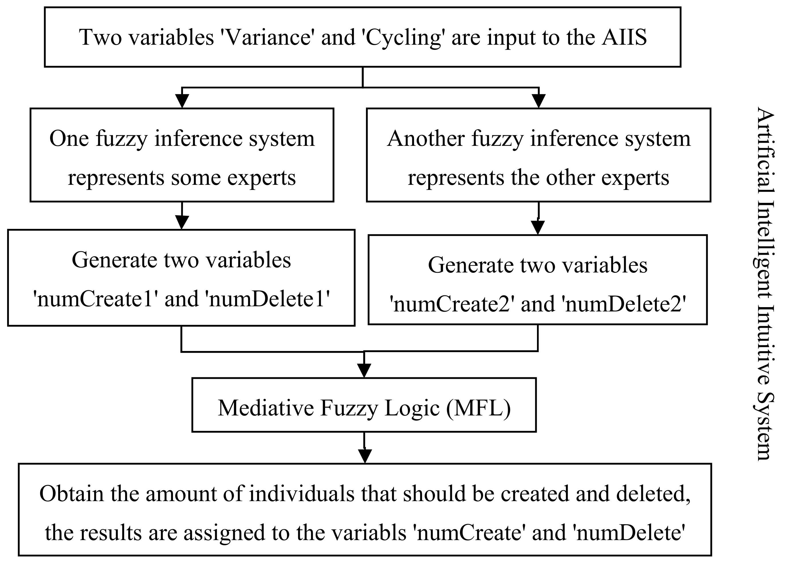
3.1.2. The Artificial Intelligent Intuitive System

AIIS is used to calculate the number of individuals that should be created or deleted in the actual population based in MFL so as to adjust the population size with the purpose of accelerating the convergence of HEM. The MFL uses two variables in AIIS named ‘variance’ and ‘cycling’ which are obtained by using the fitness value of the best individual of previous generations. Additionally, two variables named ‘numCreate’ and ‘numDelete’ are used to save the number of individuals that should be generated and eliminated. The process of AIIS is shown in Figure 1. See Reference [40,41] for more detailed information about AIIS.

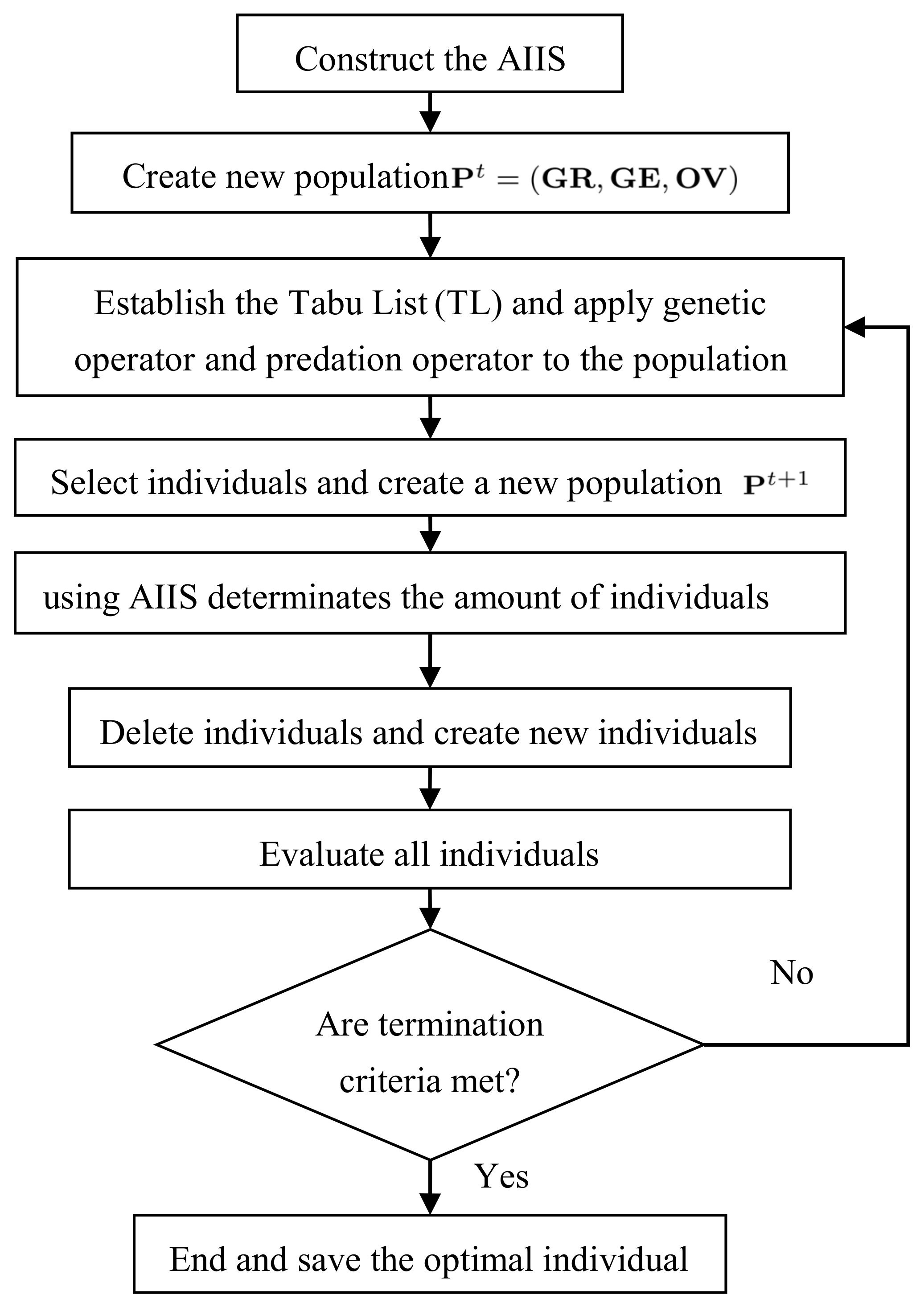
3.2. The Idea of the Proposed Algorithm

An algorithm was proposed for solving the BLPP based the HEM combined with the decision-making process of the BLPP. The genetic representation of each individual depends on the upper and lower solution rather than only one decision maker, so the lower maker passes on the relevant optimal solutions to the upper to construct the individual genetic representation. The lower level problem can be regarded as a common nonlinear programming problem under the circumstances that the upper level decision variable is given. Therefore, in the presented algorithm, the HEM focuses on the upper level problem and controls the evolution tendency for two level problems while the lower level problem is dealt with by GA.

To solve the BLPP using the HEM, we redefine how to generate the individuals. Firstly, let us define the following:

• $x={(x_1,x_2,\cdots ,x_{n_x})}^T$: upper level decision variable,
• $y={(y_1,y_2,\cdots ,y_{n_y})}^T$: lower level decision variable,
• $F$: upper level objective function,
• $f$: lower level objective function,
• $N$: quantity of new individuals.

As mentioned above, the exhaustive process of generating new individuals is elaborated as following.

Step 1: Randomly produce the upper decision variables of size $N$ denoted by $X=(x_1,x_2,\cdots ,x_N)$. In this part the individual genetic representation cannot be defined.

Step 2: For each upper variable viewed as the known variable, solve the lower problem using genetic algorithm and obtain the relevant solution noted by $Y=(y_1,y_2,\cdots ,y_N)$. And then all the lower optimal solutions are transmitted to the upper.

Step 3: Based on X and Y, we will obtain the genetic representation of each individual $g{r}_i=(x_i^T,y_i^T)=(x_{i1},x_{i2},\cdots ,x_{i{n}_x},y_{i1},y_{i2},\cdots ,y_{i{n}_y})$, where $i=1,2,\cdots ,N$. As of this stage, we get a new population of size $N$, where the genetic representation and effect are expressed as $GR=(g{r}_1;g{r}_2;\cdots ;g{r}_N)$ and $GE=(g{e}_1;g{e}_2;\cdots ;g{e}_N)$ respectively. Moreover, we must adjust the population so as to ensure each individual meet the constraints.

Step 4: Randomly generate the genetic effect for each individual denoted by $g{e}_i=(g{e}_{i1},g{e}_{i2},g{e}_{i3},g{e}_{i4})$. Where $g{r}_{i1}$,$g{r}_{i2}$,$g{r}_{i3}$,$g{r}_{i4}$ represent individual gender, actual age, maximum age and the pheromone levels, respectively.

Step 5: Calculate the upper objective function for each individual taken as the fitness, i.e., the objective value, $ov(i)=F(g{r}_i)$. Eventually, we get the intact population shown as $P=(GR,GE,OV)$.

Each new individual is constructed according to the above steps, which are noted as $NewP$. Furthermore, the steps of the proposed algorithm are listed in details as follows.

Step 1: Initialize the parameters. Population size is set $N$, the maximum size is $ub$, the minimum size is $lb$, and the maximum generation is $M\_Gen$. At this stage, the generation is set $t=0$.

Step 2: Create an initial population of size $N$ using $NewP$ noted by $P^t$.

Step 3: For the $t\mathrm{th}$ generation, the best individual $p^{Best}$ is saved in a Tabu List (TL) which is defined as $t{l}^t$. The same individual cannot be saved in the list repeatedly. Moreover, each individual in the list $TL={\left\{t{l}^t\right\}}_{t=1}^L$ has a radius $\rho$ to represent a subspace in the search space.

Step 4: Update the population $P^t$. Genetic operator and predation operator are respectively applied to the whole population so as to control the genetic effects and genetic representations.

Step 5: Select individuals. According to the pyramidal selection rule, we select the individuals satisfying the criteria to create a new population.

Step 6: The variance of the best individual for the last generations is calculated and saved as ‘Variance’, and the variable named ‘Cycling’ is obtained according to that value. After that, we will get the quantity of individuals that will be eliminated and create respectively named ‘Delete’ and ‘Create’ using AIIS based on the two variables.

Step 7: Eliminate the individuals with less fitness in accordance with the variable ‘Delete’, as well as create some new individuals in view of the variable ‘Create’ using TS.

Step 8: If the terminal condition is fulfilled, save the optimal individual. The genetic representation of this individual is the optimal solution and the objective value is optima of the upper. If not, go to Step 3.

According to the steps mentioned above, the flow chart of the proposed algorithm is shown in the following Figure 2.

4. Computational Experiments

In order to illustrate the feasibility and efficiency of the proposed algorithm, four examples from references are presented to carry out the numerical experiment.

Example 1 [3]:

$$\begin{array}{l}\underset{x,y}{\min } F(x,y)=-8x_1-4x_2+4y_1-40y_2-4y_3\hfill \\ s.t. x\ge 0,\hfill \\ \mathrm{where} y \mathrm{solves} :\hfill \\ \underset{y}{\min } f(x,y)=x_1+2x_2+y_1+y_2+2y_3\hfill \\ s.t. -y_1+y_2+y_3\le 1, \hfill \\ 2x_1-y_1+2y_2-0.5y_3\le 1,\hfill \\ 2x_2+2y_1-y_2-0.5y_3\le 1, y\ge 0.\hfill \end{array}$$

(1)

Example 2 [48]:

$$\begin{array}{l}\underset{x,y}{\min } F(x,y)=x^2+{(y-10)}^2\hfill \\ s.t. -x+y\le 0, 0\le x\le 15,\hfill \\ \mathrm{where} y \mathrm{sovles}:\hfill \\ \underset{y}{\min } f(x,y)={(x+2y-30)}^2\hfill \\ s.t. x+y\le 20, 0\le y\le 20.\hfill \end{array}$$

(2)

Example 3 [49]:

$$\begin{array}{l}\underset{x,y}{\min } F(x,y)=\left|2x_1+2x_2-3y_1-3y_2-60\right|\hfill \\ s.t. x_1+x_2+y_1-2y_2\le 40, 0\le x\le 50,\hfill \\ \mathrm{where} \mathrm{y} \mathrm{solves}:\hfill \\ \underset{y}{\min } f(x,y)={(y_1-x_1+20)}^2+{(y_2-x_2+20)}^2\hfill \\ s.t. 2y_1-x_1+10\le 0, 2y_1-x_2+10\le 0,\hfill \\ -10\le y\le 20\hfill \end{array}$$

(3)

Example 4 [30]:

$$\begin{array}{l}\underset{x,y}{\min } F(x,y)={\displaystyle \sum _{i=1}^{10}\left[\left|x_i-1\right|+\left|y_i\right|\right]}\\ \mathrm{where} \mathrm{y} \mathrm{solves}:\\ \underset{y}{\min }f(x,y)=\exp \left\{\left[1+{\displaystyle \sum _{i=1}^{10}(y_i^2/4000)}-{\displaystyle \prod _{i=1}^{10}cos(y_i/\sqrt{i})}\right]{\displaystyle \sum _{i=1}^{10}{x}_i^2}\right\}\\ s.t. -\pi \le y\le \pi \end{array}$$

(4)

We choose four typical examples (e.g., involving linear, quadratic and other nonlinear cases) to illustrate the feasibility of the proposed algorithm. Moreover, the objective functions of Example 3 and Example 4 are not convex and differentiable as well. Example 4 is a large-scale problem with 10 decision variables for both upper and lower problem, respectively. The general features of those examples are shown in

Table 1. The examples’ features.

No.	Type	Scale	Functions
Example 1	Linear	$n=2,m=3$	Convex and differentiable
Example 2	quadratic	$n=1,m=1$	Convex and differentiable
Example 3	nonlinear	$n=2,m=2$	Non-convex and non-differentiable
Example 4	nonlinear	$n=10,m=10$	Non-convex and non-differentiable

.

4.1. The Parameters of the Algorithm

The parameters setting process is divided into three parts. Firstly, the AIIS viewed as an essential step for the proposed algorithm to establish is established using the method presented by Montiel et al. in Reference [44]. Secondly, the parameters related to population are chosen such as the initial, max, and min population size, the max iterations and the max age for each individual. Thirdly, some parameters relevant to the genetic and predation operations in HEM are set referring to Reference [44]. The detailed values of these parameters are demonstrated in

Table 2. Parameters of the algorithm.

	Recombination	Mutation		Max Age	Population Size			Iteration
		K	λ		Initial	Min	Max	Max	Min
Example 1	0.25	16	0.1	10	50	20	150	100	30
Example 2			0.1	20	50	30	200	150	50
Example 3			0.5	5	80	50	150	100	30
Example 4			0.5	8	80	50	200	200	50

. For more specifications on these parameters, consult Reference [44]. Additionally, for the presented algorithm, the termination criteria is met if the iteration exceeded the maximal number of generation, the value of the fitness function did not change in 5 generations or magnitude of step is smaller than 10⁻⁵. For all experiments, the algorithm is executed in a personal computer with 4.0 GB RAM and Windows 7 operating system. For convenience, the GA is coded in virtue of GA toolbox in Matlab because the algorithm is implemented in MATLAB.

As for GA used in this algorithm for all experiments, the parameter setting is employed: Each individual is stochastically initialized utilizing real-number encoding; the maximal number of iterations is 200 and the initial population size is 50; roulette selection, scattered crossover, and uniform mutation are implemented and the crossover fraction and mutation fraction is 0.8 and 0.01, respectively. Each experiment is terminated either when the maximal number of iterations is exceeded or when the objective of each individual does not change in 50 iterations.

4.2. Experimental Results

We execute the proposed algorithm 20 independent runs on each problem in that the result could show its performance directly. Therefore, the optimal solutions obtained by the proposed algorithm are recorded, as well as the corresponding computing time taken by the algorithm are listed in

Table 3. Statistics of the iteration and computing time.

	Example 1		Example 2		Example 3		Example 4
	Iterations	Time (s)	Iterations	Time (s)	Iterations	Time (s)	Iterations	Time (s)
Min(best)	51	11.289	50	300.404	20	173.885	200	38,024.21
Max	60	32.534	64	2058.331	41	8082.929	200	39,149.43
Average	54.5	19.889	54.4	1125.779	27.9	1054.349	200	38,586.82

. Moreover, the comparison of the solutions by the proposed algorithm with those in related references is demonstrated in

Table 4. Comparison of the solutions by the proposed algorithm with those in related references.

		Our Proposed Algorithm	Reference: Wan et al.	Reference
Example 1	$F$	−29.199879	−29.200009	−29.2
	$f$	3.199977	3.200009	3.2
	$x$	(0,0.899997)	(2 × 10−6,0.899997)	(0,0.9)
	$y$	(1.92 × 10−12,0.599998,0.399992)	(4 × 10−6,0.6,0.400005)	(0,0.6,0.4)
Example 2	$F$	100	100.01	100.58
	$f$	5.72 × 10−16	2.5 × 10−7	0.01
	$x$	10	10.0005	10.03
	$y$	10	9.9995	9.969
Example 3	$F$	5.85 × 10−7	0	0
	$f$	100	100	100
	$x$	(0,29.999999)	(0,30)	(0,30)
	$y$	(−9.999999,9.999999)	(−10,10)	(−10,10)
Example 4	$F$	3.26 × 10−3	0	6.21 × 10−4
	$f$	1	1	1
	$x$	(1.000087,1.000387, 1.000230,1.000338, 1.000190,0.999098, 1.000254,0.999878, 1.000146,1.000592)	(1, 1, 1, 1, 1, 1, 1, 1, 1, 1)	(0.99999998, 0.99999999, 1.00000006,0.99999999, 1.00000000,1.00000001, 0.99999999,0.99999992, 0.99999998, 1.00000001)
	$y$	(3.56 × 10−6,−2.11 × 10−7,7.38 × 10−7, 5.02 × 10−7,−5.38 × 10−7,−1.26 × 10−6, −9.99 × 10−7,−2.30 × 10−6,−9.08 × 10−8, 1.71 × 10−6)	(0, 0, 0, 0, 0, 0, 0, 0, 0, 0)	1.0 × 10−3 (−0.04845,−0.03471, 0.11674,0.09264,0.2121, 0.09969,0.07125,0.05798,0.04344,0.03512)

.

As to the performance of the proposed algorithm, the computing time and iteration show the feasibility and stability of the algorithm to some extent. Obviously, it can be seen from Table 3 that the iteration and computing time with little change illustrate the presented algorithm is generally feasible and steady for all examples. In concrete terms, it is worth noticing that the computing time for Example 1 is less than others due to its small scale which at least shows the feasibility of the proposed algorithm. For Example 4, on the contrary, it is a large-scale problem, so it has the most computing time and iteration. However, it is notable that the computing times in Example 1 and 4 vary in a small interval, which also demonstrates the algorithm is steady during these numerical experiments. Furthermore, as to Example 2 and Example 3, it can be seen that the fluctuation in the iteration is tiny, but the corresponding computing time varies greatly. The reason is that the population is initialized randomly and the population size is adaptively adjusted; what is more, the range of the size is not strictly limited to a small interval so that the amount of the individuals may vary greatly for each run. Finally, as for the small-scale examples (Example 1, 2, and 3), the maximal iterations are much less than the maximum setting value of the corresponding parameter, which also illustrates the efficiency and feasibility of the constructed algorithm is acceptable. Meanwhile, it is undeniable that for Example 4, the iteration parameter is up to the maximum setting value of the related parameter indicating that the presented algorithm should be improved to efficiently solve larger-scale problems. Overall, these results indicate that the proposed algorithm is feasible and stable for all experiments. Next, the optima obtained by the novel algorithm is compared with the existing studies to show its performance in detail.

In Table 4, Column ‘Reference Wan et al.’ lists the results given by Wan et al. for all examples, and Column ‘Reference’ sequentially lists the results obtained by Bard for Example 1 [3], Oduguwa and Roy for Example 2 [48], Craenen and Eiben for Example 3 [49], Wang et al. for Example 4 [30]. According to the comparison of the results in Table 4, it can be observed that the solutions obtained by our algorithm for Example 2 is better than those produced by the compared algorithms in the references. For this situation, we can draw a primary conclusion that the presented algorithm is capable to improve the current algorithm. However, as for Example 1, the upper objective function in this paper are a little worse than these given by the compared algorithms while the results of the lower objective function are better than in the existing researches. This situation manifests that the conflicting goal among the upper and lower level indeed exist from another angle and also prove the presented algorithm is feasible.

Furthermore, for Example 4, our results are a little worse than those presented by Wan et al. [50], whilst it is very similar to those obtained by Wang et al. [30]. These situations again show that the presented algorithm can solve large scale problems but the calculation accuracy should be improved to get more precise results. Besides, as to Example 3, the results yielded by the proposed algorithm are almost equal to those in the current research excluding the accuracy difference in the lower objective function, which emphasizes the accuracy of our algorithm needs to be enhanced. Generally, it can be concluded that within the acceptable precision, the solutions for all examples by our algorithm are close enough to the global optimal solutions found in the references.

5. Conclusions

In this paper, we present an algorithm for solving bilevel programming problem based on the simplified human evolutionary model. Furthermore, we design the algorithm combined with the decision process of the BLPP. Consequently, the BLPP needs not to be transformed to another form in terms of the presented algorithm so that there is no restriction on the nature of the problem, so it can be widely used to solve more various actual problems.

Based on the numerical results compared with those in corresponding references, the following could be concluded:

(1)

The proposed algorithm is feasible for various bilevel programming problems such as linear, quadratic and nonlinear problems. Our method does not impose any restriction on the problems.

(2)

The evolution is basically stable in our method because of the consistent iterations in each run for all examples.

(3)

Although in some cases the solutions by our algorithm are not so good as the compared algorithms, within the acceptable precision, the algorithm can converge to the global optima and the solutions are completely acceptable.

Generally speaking, the precision of our method needs to be improved. In our future works, the following will be researched:

(1)

We still plan to do more research about the influence of the parameters on the performance so as to control more parameters adaptively using AIIIS and simply the HEM on the basis of the basic HEM.

(2)

Many more and larger-scale problems will be solved to demonstrate the efficiency of our proposed algorithm.

(3)

Comparison with other algorithms by solving more examples will also be our future work to illustrate the superiority of our algorithm.

References

1. Aghajani, S.; Kalantar, M. Operational scheduling of electric vehicles parking lot integrated with renewable generation based on bilevel programming approach. Energy 2017, 139, 422–432. [Google Scholar] [CrossRef]
2. Labbe, M.; Violin, A. Bilevel programming and price setting problems. Ann. Oper. Res. 2016, 240, 141–169. [Google Scholar] [CrossRef]
3. Bard, F. Practical Bilevel Optimization: Algorithms and Applications; Kluwer Academic Publishers: Dordrecht, The Netherlands, 1998. [Google Scholar]
4. Vicente, L.; Calamai, P.H. Bilevel and multibilevel programming: A bibliography review. Glob. Optim. 1994, 5, 291–306. [Google Scholar] [CrossRef]
5. Dempe, S. Foundations of Bilevel Programming; Kluwer Academic Publishers: Dordrecht, The Netherlands, 2002. [Google Scholar]
6. Dempe, S. Annotated bibliography on bilevel programming and mathematical programs with equilibrium constraints. Optimization 2003, 52, 333–359. [Google Scholar] [CrossRef]
7. Colson, B.; Marcotte, P.; Savard, G. An overview of bilevel optimization. Ann. Oper. Res. 2007, 153, 235–256. [Google Scholar] [CrossRef]
8. Wang, G.M.; Wang, Z.P.; Wang, X. An overview of two(bi)-level programming review. Adv. Math. 2007, 36, 513–529. [Google Scholar]
9. Huang, Z.; Yang, C.; Zhou, X.; Gui, W. A novel cognitively inspired state transition algorithm for solving the linear Bi-level programming problem. Cogn. Comput. 2018, 10, 816–826. [Google Scholar] [CrossRef]
10. Jeroslow, R.G. The polynomial hierarchy and a simple model for competitive analysis. Math. Program. 1985, 32, 146–164. [Google Scholar] [CrossRef]
11. Ben-Ayed, O.; Blair, C. Computational difficulties of bilevel linear programming. Oper. Res. 2012, 38, 556–560. [Google Scholar] [CrossRef] [Green Version]
12. Bard, F. Some properties of the bilevel linear programming problem. J. Optim. Theory Appl. 1991, 68, 146–164. [Google Scholar] [CrossRef]
13. Vicente, L.; Savard, G.; Judice, J. Descent approaches for quadratic bilevel programming. J. Optim. Theory Appl. 1994, 81, 379–399. [Google Scholar] [CrossRef]
14. Deng, X. Complexity issues in bilevel linear programming. In Multilevel Optimization: Algorithms and Applications; Migdalas, A., Pardalos, P.M., Varbrand, P., Eds.; Kluwer Academic Publishers: Dordrecht, The Netherlands, 1998; pp. 149–164. [Google Scholar]
15. Li, T.; Chen, C.Y.; Su, W.L. Plant growth simulation algorithm for solving bilevel programming. Oper. Res. Manag. Sci. 2012, 21, 123–128. [Google Scholar]
16. Watada Roy, A.; Li, R.; Wang, B.; Wang, S. A dual recurrent neural network-based hybrid approach for solving convex quadratic Bi-level programming problem. Neurocomputing 2020, 407, 136–154. [Google Scholar] [CrossRef]
17. Yi, Z.K.; Xu, Y.L.; Sun, H.B. Self-adaptive hybrid algorithm based bi-level approach for virtual power plant bidding in multiple retail markets. IET Gener. Transm. Distrib. 2020, 14, 3762–3773. [Google Scholar] [CrossRef]
18. Abo-Elnaga, Y.; Nasr, S. Modified evolutionary algorithm and chaotic search for bilevel programming problems. Symmetry 2020, 12, 767. [Google Scholar] [CrossRef]
19. Fateh, H.; Bahramara, S.; Safari, A. Modeling operation problem of active distribution networks with retailers and microgrids: A multi-objective bi-level approach. Appl. Soft Comput. 2020, 94, 106484. [Google Scholar] [CrossRef]
20. Luo, H.; Liu, L.; Yang, X. Bi-level programming problem in the supply chain and its solution algorithm. Soft Comput. 2020, 24, 2703–2714. [Google Scholar] [CrossRef]
21. Zhang, T.; Chen, Z.; Chen, W. A cooperative coevolution PSO technique for complex bilevel programming problems and application to watershed water trading decision making problems. J. Nonlinear Sci. Appl. 2017, 10, 2115–2132. [Google Scholar] [CrossRef] [Green Version]
22. Tang, Q.; Fu, Z.; Qiu, M. A bilevel programming model and algorithm for the static bike repositioning problem. J. Adv. Transp. 2019. [Google Scholar] [CrossRef] [Green Version]
23. Abo-Elsayed, Y.; El-Shorbagy, M.A. Multi-sine cosine algorithm for solving nonlinear bilevel programming problems. Int. J. Comput. Intell. Syst. 2020, 13, 421–432. [Google Scholar]
24. Zhang, T.; Liu, R.L.; Chen, F. The BP artificial neural network based on elite PSO algorithm for general bilevel programming problems. J. Nonlinear Convex Anal. 2020, 21, 885–898. [Google Scholar]
25. Feng, Q.; Qin, S.T.; Shi, F.L.; Zhao, S. A recurrent neural network with finite-time convergence for convex quadratic bilevel programming problems. Neural Comput. Appl. 2018, 30, 3399–3408. [Google Scholar] [CrossRef]
26. Zhang, T.; Li, X.F. The backpropagation artificial neural network based on elite particle swam optimization algorithm for stochastic linear bilevel programming problem. Math. Probl. Eng. 2018. [Google Scholar] [CrossRef] [Green Version]
27. Zhu, Z.C.; Yu, B. A modified homotopy method for solving the principal-agent bilevel programming problem. Comput. Appl. Math. 2018, 37, 541–566. [Google Scholar] [CrossRef]
28. Sinha, A.; Malo, P.; Deb, K. An improved bilevel evolutionary algorithm based on Quadratic Approximations. In Proceedings of the 2014 IEEE Congress on Evolutionary Computation (CEC), Beijing, China, 6–11 July 2014; pp. 1870–1877. [Google Scholar]
29. Lin, D.; Chou, Y.Z.; Li, M.Q. Multi-objective evolutionary algorithm for multi-objective bi-level programming problems. J. Syst. Eng. 2007, 22, 182–186. [Google Scholar]
30. Wang, Y.; Li, H.; Dang, C. A new evolutionary algorithm for a class of nonlinear bilevel programming problems and its global convergence. Inf. J. Comput. 2011, 23, 618–629. [Google Scholar] [CrossRef]
31. Rodriguez, F.; Lozano, M.; Garcia-Martinez, C.; García-Martínez, J.D. An artificial bee colony algorithm for the maximally diverse grouping problem. Inf. Sci. 2013, 320, 183–196. [Google Scholar] [CrossRef]
32. Calvete, H.I.; Gale, C.; Oliveros, M. Bilevel model for production-distribution planning solved by using ant colony optimization. Comput. Oper. Res. 2011, 38, 320–327. [Google Scholar] [CrossRef]
33. Wang, G.M.; Ma, L.M. The estimation of particle swarm distribution algorithm with sensitivity analysis for solving nonlinear bilevel programming problems. IEEE Access 2020, 8, 137133–137149. [Google Scholar] [CrossRef]
34. Montiel, O.; Castillo, O.; Rodríguez, A.; Melin, P.; Sepúlveda, R. Human evolutionary model: A new approach to optimization. Inf. Sci. 2007, 177, 2075–2098. [Google Scholar] [CrossRef]
35. Candler, W.; Norton, R. Multilevel Programming; Technical Report 20; World Bank Development Research Center: Washington, DC, USA, 1977. [Google Scholar]
36. Candler, W.; Townsley, R. A linear two-level programming problem. Comput. Oper. Res. 1982, 9, 59–76. [Google Scholar] [CrossRef]
37. Bialas, W.F.; Karwan, M.H. On two-level optimization. IEEE Trans. Autom. Control 1982, 7, 211–214. [Google Scholar] [CrossRef]
38. Bialas, W.F.; Karwan, M.H. Two-level linear programming. Manag. Sci. 1984, 30, 1004–1020. [Google Scholar] [CrossRef]
39. Bard, F. Geometric and algorithmic developments for a hierarchical planning problem. Eur. J. Oper. Res. 1985, 19, 372–383. [Google Scholar] [CrossRef]
40. Montiel, O.; Castillo, O. Mediative fuzzy logic: A novel approach for handling contradictory knowledge. In Hybrid Intelligent Systems; Springer: Berlin/Heidelberg, Germany, 2007; pp. 75–91. [Google Scholar]
41. Montiel, O.; Castillo, O.; Melin, P.; Sepulveda, R. Mediative fuzzy logic: A new approach for contradictory knowledge management. In Forging New Frontiers: Fuzzy Pioneers II; Springer: Berlin/Heidelberg, Germany, 2008; pp. 135–149. [Google Scholar]
42. Atanassov, K.T. Intuitionistic fuzzy sets: Past, present and future. In Proceedings of the 3rd Conference of the European Society for Fuzzy Logic and Technology, Zittau, Germany, 10–12 September 2003; pp. 12–19. [Google Scholar]
43. Li, D.F. Intuitionistic Fuzzy Set Theories Decision and Game Theory in Management with Intuitionistic Fuzzy Sets; Springer: Berlin/Heidelberg, Germany, 2014; pp. 1–12. [Google Scholar]
44. Montiel Ross, O.H.; Castillo, O.; Melin, P.; Sepúlveda, R. Mediative fuzzy logic: A novel approach for handling contradictory knowledge. In Proceedings of the International Conference on Fuzzy Systems, Neural Networks and Genetic Algorithms (FNG 2005), Tijuana, Mexico, 13–14 October 2005. [Google Scholar]
45. Montiel, O.; Castillo, O.; Melin, P.; Sepúlveda, R. Improving the human evolutionary model: An intelligent optimization method. Int. Math. Forum 2007, 2, 21–44. [Google Scholar] [CrossRef] [Green Version]
46. Montiel, O.; Castillo, O.; Melin, P.; Sepúlveda, R. Reducing the cycling problem in evolutionary algorithm. In Proceedings of the 2005 International Conference on Artificial Intelligence, Las Vegas, NV, USA, 27–30 June 2005; pp. 426–432. [Google Scholar]
47. Castillo, O.; Melin, P. A new method for fuzzy inference in intuitionistic fuzzy systems. In Proceedings of the International Conference NAFIPS 2003, Chicago, IL, USA, 24–26 July 2003; IEEE Press: Chicago, IL, USA, 2003; pp. 20–25. [Google Scholar]
48. Oduguwa, V.; Roy, R. Bi-level optimisation using genetic algorithm. In Proceedings of the 2002 IEEE International Conference on Artificial Intelligence Systems (ICAIS 2002), Divnomorskoe, Russia, 5–10 September 2002; pp. 322–327. [Google Scholar]
49. Wang, Y.; Iao, Y.; Li, H. An evolutionary algorithm for solving nonlinear bilevel programming based on a new constraint-handling scheme. IEEE Trans. Syst. Man Cybern. Part C Appl. Rev. 2005, 35, 221–232. [Google Scholar] [CrossRef]
50. Wan, Z.P.; Mao, L.; Wang, G.M. Estimation of distribution algorithm for a class of nonlinear bilevel programming problems. Inf. Sci. 2014, 256, 184–196. [Google Scholar] [CrossRef]
Figure 1. Process of adaptive intelligent/intuitive system (AIIS).
Algorithms 13 00260 g001
Figure 2. Flow chart of the proposed algorithm.
Algorithms 13 00260 g002