Simple Constructive, Insertion, and Improvement Heuristics Based on the Girding Polygon for the Euclidean Traveling Salesman Problem

 , ,
, , 
Abstract
1. Introduction
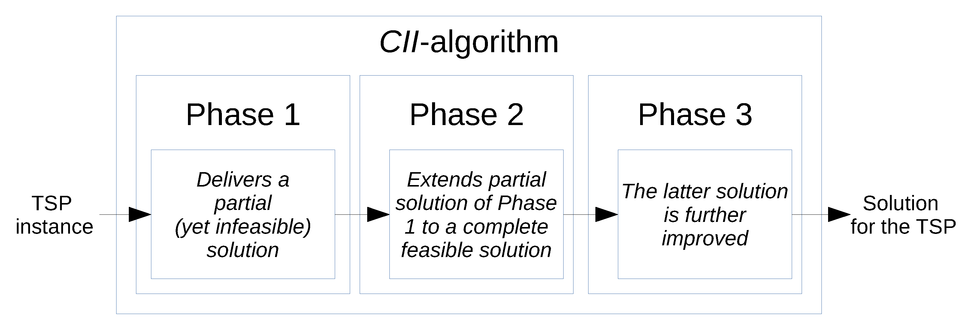
2. Methods
2.1. Phase 1
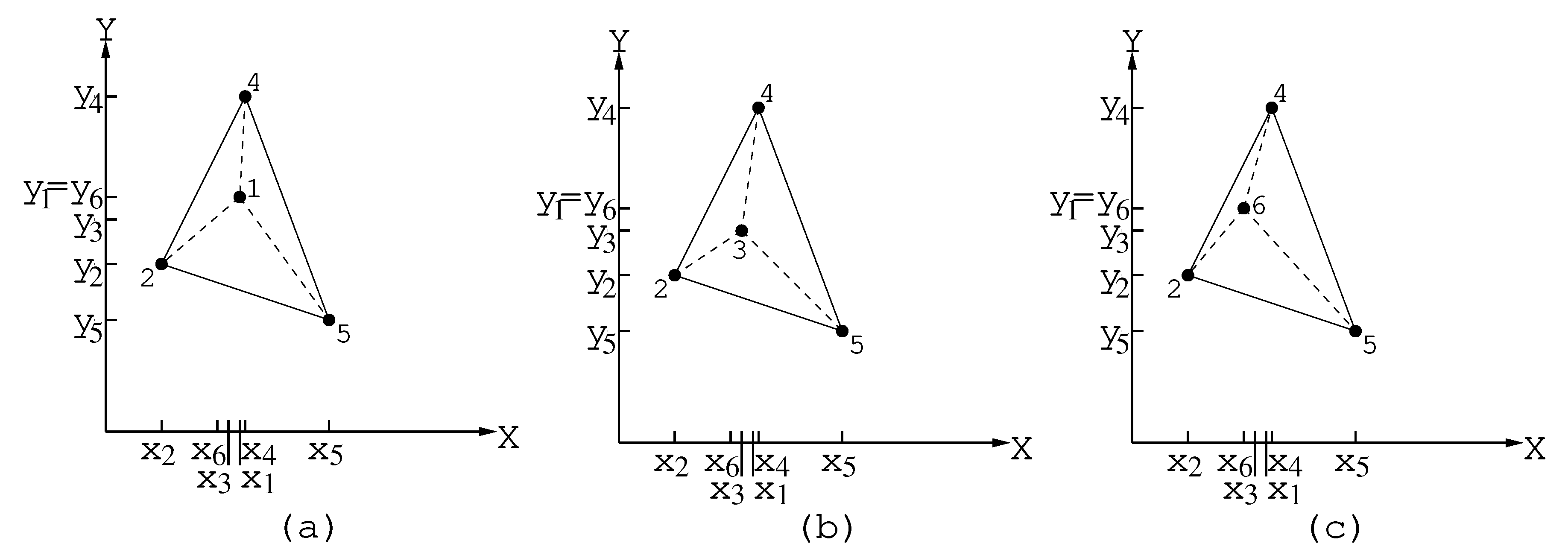
2.1.1. Procedure to Locate the Extreme Points
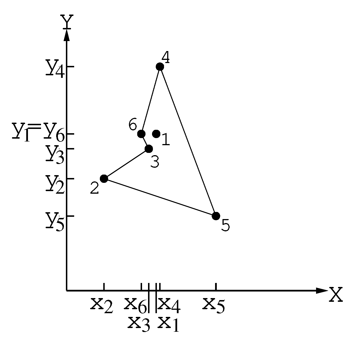
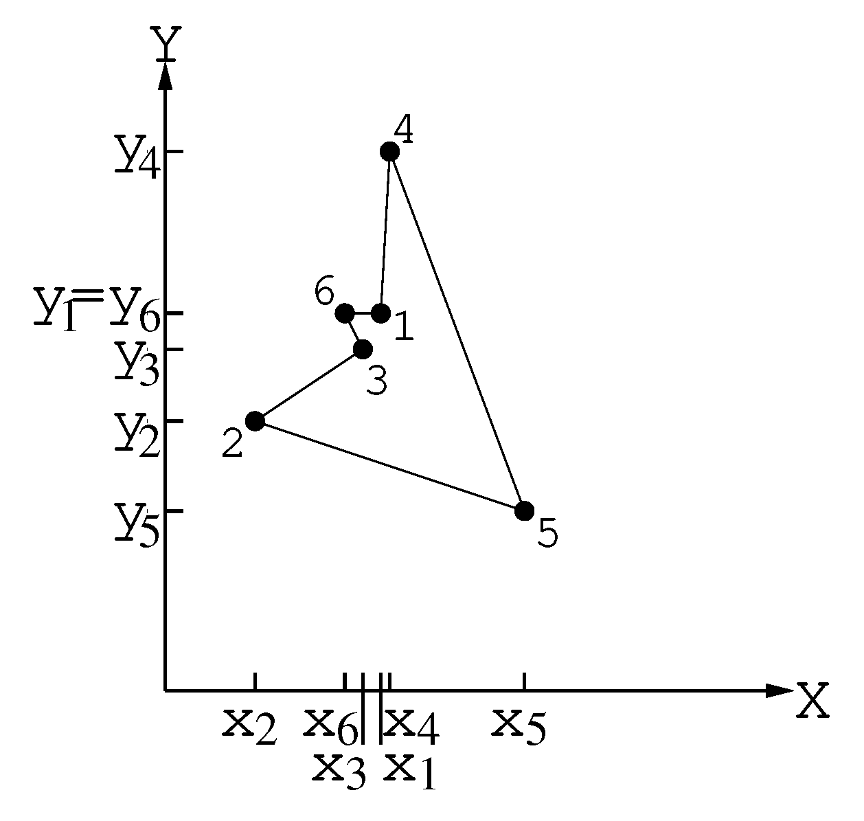
2.1.2. Procedure for the Construction of the Girding Polygon
2.2. Phase 2
Procedure Construc_tour
2.3. Phase 3
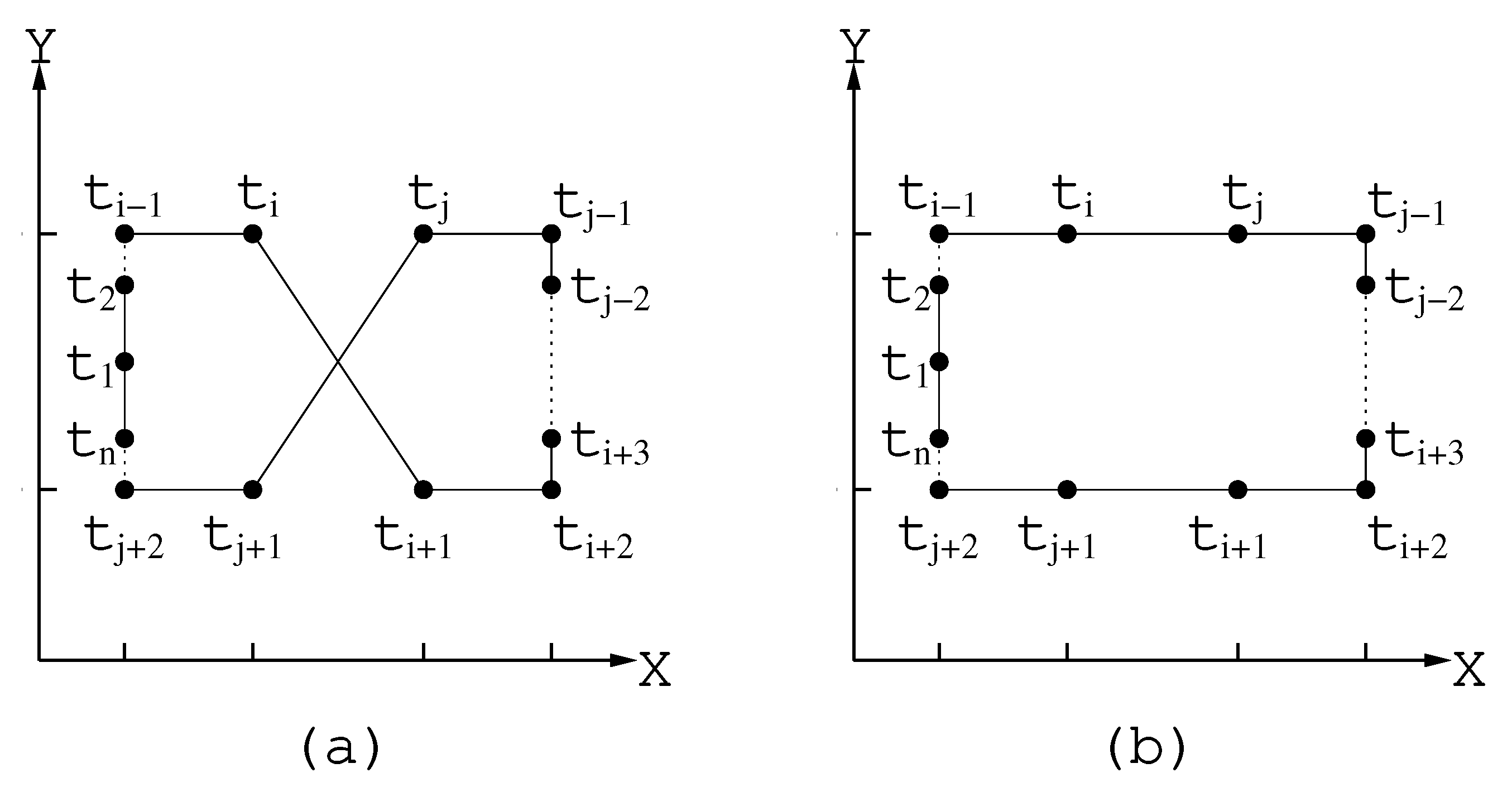
2.3.1. Procedure 2-Opt
2.3.2. Procedure improve_tour
3. Implementation and Results
4. Conclusions and Future Work
Author Contributions
Funding
Conflicts of Interest
Appendix A

| Heuristic Id | Heuristic Name | Number of Reported Instances | Runs |
|---|---|---|---|
| ACO-RPMM [9] | ACO - Restricted Pheromone Matrix Method | 6 Large | 10 |
| Partial ACO [6] | Partial ACO | 4 Large and 5 Small | 100 |
| DFACO [10] | Dynamic Flying ACO | 30 Small | 100 |
| ACO-3Opt [10] | ACO-3Opt | 30 Small | 100 |
| DPIO [12] | Discrete Pigeon-inspired optimization with Metropolis acceptance | 1 Large, 6 Medium and 28 Small | 25 |
| PACO-3Opt [8] | Parallel Cooperative Hybrid Algorithm ACO | 21 Small | 20 |
| ESACO [7] | Effective Strategies + ACO | 5 Medium and 17 Small | 20 |
| PRNN [11] | Parallel Repetitive Nearest Neighbor | 3 Medium and 9 Small | |
| NN | Nearest Neighbor Algorithm | 4 Large, 25 Medium and 61 Small | 1 |
| Header | Header Description |
|---|---|
| the number of vertices in the instance | |
| Opt? | “yes” if Best Known Solution (BKS) is optimal, “no” otherwise |
| the cost of BKS | |
| Cost of the solution constructed by CII heuristic | |
| RAM | RAM used by CII heuristics |
| # | the number of cycles at Phase 3 of CII heuristic |
| Error | as defined in Formula (13) |
| the average cost of the solution obtained by heuristic H | |
| Heuristic Id | nomenclature used in Table A1 |
| Time | the processing time of a heuristic |
| ms, s, m, h, d | time units for milliseconds, seconds, minutes, hours and days respectively. |
| Instance | CII Heuristic (Phase 2) | CII Heuristic (Phase 3) | Other Heuristics | ||||||||||||
|---|---|---|---|---|---|---|---|---|---|---|---|---|---|---|---|
| V | Opt? | Time | Time | RAM | # | Time | Heuristic Id | ||||||||
| eil51 | 51 | yes | 426 | 454 | 6.6% | 0.4 ms | 454 | 6.6% | 1.0 ms | 0.5 MiB | 1 | 426 | 0.0% | 1.0 s | DFACO |
| 426 | 0.0% | 1.0 s | ACO-3Opt | ||||||||||||
| 426 | 0.0% | 1.1 s | ESACO | ||||||||||||
| berlin52 | 52 | yes | 7542 | 8058 | 6.8% | 1.1 ms | 8058 | 6.8% | 4.5 ms | 0.6 MiB | 3 | 7542 | 0.0% | 1.0 s | DFACO |
| 7542 | 0.0% | 1.0 s | ACO-3Opt | ||||||||||||
| st70 | 70 | yes | 675 | 710 | 5.2% | 0.6 ms | 701 | 3.8% | 11.1 ms | 0.6 MiB | 3 | 826 | 22.3% | 0.4 ms | NN |
| eil76 | 76 | yes | 538 | 576 | 7.0% | 0.7 ms | 556 | 3.4% | 2.2 ms | 0.6 MiB | 3 | 538 | 0.0% | 3.0 s | DFACO |
| 538 | 0.0% | 3.0 s | ACO-3Opt | ||||||||||||
| 538 | 0.0% | 1.4 s | ESACO | ||||||||||||
| pr76 | 76 | yes | 108,159 | 114,808 | 6.1% | 0.7 ms | 112,911 | 4.4% | 3.0 ms | 0.6 MiB | 4 | 148,348 | 37.2% | 0.5 ms | NN |
| rat99 | 99 | yes | 1211 | 1294 | 6.9% | 1.0 ms | 1230 | 1.5% | 9.4 ms | 0.6 MiB | 3 | 1442 | 19.1% | 0.8 ms | NN |
| kroA100 | 100 | yes | 21,282 | 23,050 | 8.3% | 1.1 ms | 21,443 | 0.8% | 3.5 ms | 0.6 MiB | 3 | 21,282 | 0.0% | 2.0 s | DFACO |
| 21,282 | 0.0% | 2.0 s | ACO-3Opt | ||||||||||||
| 21,282 | 0.0% | 2.6 s | ESACO | ||||||||||||
| kroB100 | 100 | yes | 22,141 | 23,247 | 5.0% | 1.1 ms | 22,716 | 2.6% | 3.3 ms | 0.6 MiB | 3 | 22,141 | 0.0% | 2.0 s | DFACO |
| 22,141 | 0.0% | 2.0 s | ACO-3Opt | ||||||||||||
| kroC100 | 100 | yes | 20,749 | 21,632 | 4.3% | 1.1 ms | 20,922 | 0.8% | 3.8 ms | 0.6 MiB | 3 | 20,749 | 0.0% | 2.0 s | DFACO |
| 20,749 | 0.0% | 2.0 s | ACO-3Opt | ||||||||||||
| kroD100 | 100 | yes | 21,294 | 21,712 | 2.0% | 1.1 ms | 21,582 | 1.4% | 3.4 ms | 0.6 MiB | 3 | 21,294 | 0.0% | 3.0 s | DFACO |
| 21,294 | 0.0% | 3.0 s | ACO-3Opt | ||||||||||||
| kroE100 | 100 | yes | 22,068 | 22,870 | 3.6% | 1.0 ms | 22,528 | 2.1% | 8.3 ms | 0.6 MiB | 3 | 22,068 | 0.0% | 2.0 s | DFACO |
| 22,068 | 0.0% | 2.0 s | ACO-3Opt | ||||||||||||
| rd100 | 100 | yes | 7910 | 8465 | 7.0% | 1.2 ms | 8245 | 4.2% | 3.8 ms | 0.6 MiB | 3 | 7910 | 0.0% | 2.0 s | DFACO |
| 7910 | 0.0% | 2.0 s | ACO-3Opt | ||||||||||||
| eil101 | 101 | yes | 629 | 679 | 7.9% | 1.1 ms | 666 | 5.9% | 19.5 ms | 0.6 MiB | 3 | 629 | 0.0% | 12.0 s | DFACO |
| 629 | 0.0% | 10.0 s | ACO-3Opt | ||||||||||||
| lin105 | 105 | yes | 14,379 | 14,913 | 3.7% | 1.2 ms | 14,440 | 0.4% | 3.8 ms | 0.6 MiB | 3 | 14,379 | 0.0% | 2.0 s | DFACO |
| 14,379 | 0.0% | 2.0 s | ACO-3Opt | ||||||||||||
| 14,379 | 0.0% | 2.0 s | ESACO | ||||||||||||
| pr107 | 107 | yes | 44,303 | 45,730 | 3.2% | 1.1 ms | 45,262 | 2.2% | 18.1 ms | 0.6 MiB | 5 | 54,121 | 22.2% | 0.9 ms | NN |
| pr124 | 124 | yes | 59,030 | 62,193 | 5.4% | 1.4 ms | 60,055 | 1.7% | 5.3 ms | 0.6 MiB | 3 | 73,008 | 23.7% | 1.3 ms | NN |
| bier127 | 127 | yes | 118,282 | 121,544 | 2.8% | 5.4 ms | 121,544 | 2.8% | 5.6 ms | 0.6 MiB | 3 | 118,282 | 0.0% | 47.0 s | DFACO |
| 118,282 | 0.0% | 56.0 s | ACO-3Opt | ||||||||||||
| ch130 | 130 | yes | 6110 | 6676 | 9.3% | 1.7 ms | 6190 | 1.3% | 27.9 ms | 0.6 MiB | 9 | 6110 | 0.0% | 13.0 s | DFACO |
| 6110 | 0.0% | 16.0 s | ACO-3Opt | ||||||||||||
| pr136 | 136 | yes | 96,772 | 102,934 | 6.4% | 1.7 ms | 98,711 | 2.0% | 9.9 ms | 0.6 MiB | 5 | 125,458 | 29.6% | 1.2 ms | NN |
| pr144 | 144 | yes | 58,537 | 60,625 | 3.6% | 2.1 ms | 59,902 | 2.3% | 6.8 ms | 0.6 MiB | 3 | 64,886 | 10.8% | 1.4 ms | NN |
| ch150 | 150 | yes | 6528 | 7038 | 7.8% | 2.1 ms | 6746 | 3.3% | 11.5 ms | 0.6 MiB | 3 | 6,528 | 0.0% | 24.0 s | DFACO |
| 6528 | 0.0% | 17.0 s | ACO-3Opt | ||||||||||||
| kroA150 | 150 | yes | 26,524 | 28,814 | 8.6% | 2.2 ms | 27,230 | 2.7% | 10.2 ms | 0.6 MiB | 5 | 26,524 | 0.0% | 57.0 s | DFACO |
| 26,524 | 0.0% | 1.4 m | ACO-3Opt | ||||||||||||
| kroB150 | 150 | yes | 26,130 | 27,476 | 5.2% | 2.2 ms | 26,399 | 1.0% | 26.4 ms | 0.6 MiB | 5 | 26,130 | 0.0% | 7.0 s | DFACO |
| 26,130 | 0.0% | 9.0 s | ACO-3Opt | ||||||||||||
| pr152 | 152 | yes | 73,682 | 76,952 | 4.4% | 2.3 ms | 74,605 | 1.3% | 19.0 ms | 0.6 MiB | 5 | 86,906 | 17.9% | 1.4 ms | |
| u159 | 159 | yes | 42,080 | 47,591 | 13.1% | 2.6 ms | 46,875 | 11.4% | 15.7 ms | 0.6 MiB | 3 | 53,918 | 28.1% | 1.6 ms | NN |
| rat195 | 195 | yes | 2323 | 2569 | 10.6% | 3.7 ms | 2485 | 7.0% | 16.2 ms | 0.6 MiB | 4 | 2826 | 21.7% | 2.0 ms | NN |
| d198 | 198 | yes | 15,780 | 16,862 | 6.9% | 3.9 ms | 16,119 | 2.1% | 32.6 ms | 0.6 MiB | 4 | 15,780 | 0.0% | 6.5 s | ESACO |
| kroA200 | 200 | yes | 29,368 | 31,792 | 8.3% | 3.9 ms | 30,767 | 4.8% | 17.5 ms | 0.6 MiB | 5 | 29,368 | 0.0% | 2.8 m | DFACO |
| 29,379 | 0.04% | 3.5 m | ACO-3Opt | ||||||||||||
| 29,368 | 0.0% | 4.7 s | ESACO | ||||||||||||
| kroB200 | 200 | yes | 29,437 | 32,123 | 9.1% | 3.7 ms | 30,631 | 4.1% | 11.8 ms | 0.6 MiB | 3 | 29,442 | 0.02% | 3.1 m | DFACO |
| 29,443 | 0.02% | 2.3 m | ACO-3Opt | ||||||||||||
| ts225 | 225 | yes | 126,643 | 157,163 | 24.1% | 4.5 ms | 132,803 | 4.9% | 30.6 ms | 0.6 MiB | 7 | 151,685 | 19.8% | 2.5 ms | NN |
| tsp225 | 225 | yes | 3916 | 4442 | 13.4% | 4.9 ms | 4183 | 6.8% | 22.9 ms | 0.6 MiB | 5 | 4733 | 20.9% | 2.7 ms | NN |
| pr226 | 226 | yes | 80,369 | 83,637 | 4.1% | 4.8 ms | 82,151 | 2.2% | 18.2 ms | 0.6 MiB | 3 | 94,258 | 17.3% | 2.5 ms | |
| gil262 | 262 | yes | 2378 | 2681 | 12.8% | 6.5 ms | 2539 | 6.8% | 45.4 ms | 0.6 MiB | 6 | 3102 | 30.5% | 3.4 ms | NN |
| pr264 | 264 | yes | 49,135 | 53,416 | 8.7% | 6.4 ms | 50,402 | 2.6% | 41.4 ms | 0.6 MiB | 5 | 58,615 | 19.3% | 3.6 ms | NN |
| a280 | 280 | yes | 2579 | 2686 | 4.1% | 33.6 | ms 2686 | 4.1% | 52.9 ms | 0.6 MiB | 5 | 2579 | 0.0% | 4.5 s | ESACO |
| pr299 | 299 | yes | 48,191 | 52,912 | 9.8% | 8.1 ms | 50,225 | 4.2% | 43.6 ms | 0.6 MiB | 5 | 63,254 | 31.3% | 4.3 ms | NN |
| lin318 | 318 | yes | 42,029 | 46,904 | 11.6% | 9.4 ms | 45,063 | 7.2% | 38.8 ms | 0.6 MiB | 4 | 42,228 | 0.5% | 6.4 m | DFACO |
| 42,244 | 0.5% | 5.8 m | ACO-3Opt | ||||||||||||
| 42,054 | 0.06% | 10.2 s | ESACO | ||||||||||||
| linhp318 | 318 | yes | 41,345 | 46,904 | 13.4% | 9.4 ms | 45,063 | 9.0% | 37.3 ms | 0.6 MiB | 4 | 50,299 | 21.7% | 5.1 ms | NN |
| rd400 | 400 | yes | 15,281 | 17,146 | 12.2% | 14.7 ms | 16,158 | 5.7% | 92.8 ms | 0.6 MiB | 6 | 15,384 | 0.7% | 2.2 m | PACO-3Opt |
| 15,614 | 2.2% | 24.9 m | DFACO | ||||||||||||
| fl417 | 417 | yes | 11,861 | 12,680 | 6.9% | 14.6 ms | 12,295 | 3.7% | 119 ms | 0.6 MiB | 8 | 11,880 | 0.2% | 1.6 m | PACO-3Opt |
| 11,987 | 1.1% | 34.1 m | DFACO | ||||||||||||
| pr439 | 439 | yes | 107,217 | 120,679 | 12.6% | 17.8 ms | 112,531 | 5.0% | 66.7 ms | 0.6 MiB | 3 | 107,516 | 0.3% | 2.4 m | PACO-3Opt |
| 108,702 | 1.4% | 35.5 m | DFACO | ||||||||||||
| pcb442 | 442 | yes | 50,778 | 58,746 | 15.7% | 17.7 ms | 53,275 | 4.9% | 126 ms | 0.7 MiB | 7 | 51,047 | 0.5% | 2.2 m | PACO-3Opt |
| 52,202 | 2.8% | 34.8 m | DFACO | ||||||||||||
| 50,804 | 0.05% | 11.5 s | ESACO | ||||||||||||
| d493 | 493 | yes | 35,002 | 39,050 | 11.6% | 21.8 ms | 37,045 | 5.8% | 129 ms | 0.6 MiB | 5 | 35,266 | 0.8% | 2.3 m | PACO-3Opt |
| 35,841 | 2.4% | 52.9 m | DFACO | ||||||||||||
| u574 | 574 | yes | 36,905 | 42,435 | 15.0% | 29.7 ms | 39,355 | 6.6% | 247 ms | 0.6 MiB | 9 | 37,367 | 1.3% | 1.9 m | PACO-3Opt |
| 38,031 | 3.0% | 1.5 h | DFACO | ||||||||||||
| rat575 | 575 | yes | 6773 | 7692 | 13.6% | 29.4 ms | 7215 | 6.5% | 231 ms | 0.7 MiB | 8 | 7012 | 3.5% | 1.4 h | PACO-3Opt |
| p654 | 654 | yes | 34,643 | 37,542 | 8.4% | 37.6 ms | 36,441 | 5.2% | 179 ms | 0.6 MiB | 5 | 34,741 | 0.3% | 1.7 m | DFACO |
| 35,075 | 1.2% | 2.5 h | PACO-3Opt | ||||||||||||
| d657 | 657 | yes | 48,912 | 56,268 | 15.0% | 36.7 ms | 51,553 | 5.4% | 265 ms | 0.6 MiB | 7 | 49,463 | 1.1% | 2.3 m | DFACO |
| 50,277 | 2.8% | 2.4 h | PACO-3Opt | ||||||||||||
| u724 | 724 | yes | 41,910 | 48,198 | 15.0% | 60.9 ms | 44,748 | 6.8% | 264 ms | 0.7 MiB | 6 | 42,438 | 1.3% | 2.3 m | DFACO |
| 43,122 | 2.9% | 3.2 h | PACO-3Opt | ||||||||||||
| rat783 | 783 | yes | 8806 | 10,218 | 16.0% | 54.1 ms | 9454 | 7.4% | 332 ms | 0.7 MiB | 6 | 10,492 | 19.1% | 2.5 m | DFACO |
| 10,525 | 19.5% | 15.4 m | ACO-3Opt | ||||||||||||
| 9127 | 3.6% | 4.0 h | PACO-3Opt | ||||||||||||
| 8810 | 0.04% | 22.6 s | ESACO | ||||||||||||
| dsj1000 | 1000 | yes | 18,659,688 | 21,836,514 | 17.0% | 83.6 ms | 20,225,584 | 8.4% | 460 ms | 0.7 MiB | 5 | 18,732,088 | 0.4% | 16.6 s | DPIO |
| dsj1000ceil | 1000 | yes | 18,660,188 | 21,836,514 | 17.0% | 83.5 ms | 20,225,584 | 8.4% | 452 ms | 0.6 MiB | 5 | 23,813,050 | 27.6% | 39 ms | NN |
| pr1002 | 1002 | yes | 259,045 | 295,879 | 14.2% | 87.7 ms | 276,122 | 6.6% | 744 ms | 0.7 MiB | 5 | 260,426 | 0.5% | 14.3 s | DPIO |
| 259,509 | 0.2% | 35.8 s | ESACO | ||||||||||||
| 260,366 | 0.5% | 14.1 s | DPIO | ||||||||||||
| u1060 | 1060 | yes | 224,094 | 261,093 | 16.5% | 99.5 ms | 239,705 | 7.0% | 1.0 s | 0.7 MiB | 11 | 224,932 | 0.4% | 15.3 s | DPIO |
| vm1084 | 1084 | yes | 239,297 | 275,989 | 15.3% | 104 ms | 257,399 | 7.6% | 901 ms | 0.6 MiB | 9 | 240,079 | 0.3% | 17.4 s | DPIO |
| pcb1173 | 1173 | yes | 56,892 | 67,497 | 18.6% | 124 ms | 60,792 | 6.9% | 775 ms | 0.7 MiB | 7 | 57,243 | 0.6% | 17.8 s | DPIO |
| d1291 | 1291 | yes | 50,801 | 58,230 | 14.6% | 136 ms | 54,285 | 6.9% | 927 ms | 0.7 MiB | 7 | 51,459 | 1.3% | 19.4 s | DPIO |
| rl1304 | 1304 | yes | 252,948 | 302,661 | 19.7% | 148 ms | 277,193 | 9.6% | 1.2 s | 0.7 MiB | 9 | 253,740 | 0.3% | 21.5 s | DPIO |
| rl1323 | 1323 | yes | 270,199 | 322,964 | 19.5% | 157 ms | 288,501 | 6.8% | 1.3 s | 0.7 MiB | 9 | 273,368 | 1.2% | 38.1 m | DFACO |
| 273,970 | 1.4% | 37.8 m | ACO-3Opt | ||||||||||||
| 271,245 | 0.4% | 22.2 s | ACO-3Opt | ||||||||||||
| 271,301 | 0.4% | 22.0 s | DPIO | ||||||||||||
| nrw1379 | 1379 | yes | 56,638 | 64,925 | 14.6% | 168 ms | 59,905 | 5.8% | 1.2 s | 0.7 MiB | 8 | 56,932 | 0.5% | 23.2 s | DPIO |
| fl1400 | 1400 | yes | 20,127 | 21,800 | 8.3% | 162 ms | 21,071 | 4.7% | 1.8 s | 0.7 MiB | 10 | 20,301 | 0.9% | 40.9 m | DFACO |
| 20,292 | 0.8% | 41.2 m | ACO-3Opt | ||||||||||||
| 20,342 | 1.1% | 24.6 s | ACO-3Opt | ||||||||||||
| 20,211 | 0.4% | 24.5 s | DPIO | ||||||||||||
| u1432 | 1432 | yes | 152,970 | 171,179 | 11.9% | 181 ms | 160,260 | 4.8% | 1.1 s | 0.7 MiB | 7 | 153,564 | 0.4% | 23.9 s | DPIO |
| fl1577 | 1577 | yes | 22,249 | 25,513 | 14.7% | 210 ms | 24,518 | 10.2% | 1.4 s | 0.7 MiB | 7 | 22,289 | 0.2% | 25.3 s | DPIO |
| 22,293 | 0.2% | 46.4 s | ESACO | ||||||||||||
| d1655 | 1655 | yes | 62,128 | 70,779 | 13.9% | 225 ms | 65,520 | 5.5% | 1.5 s | 0.7 MiB | 7 | 63,708 | 2.5% | 25.4 m | DFACO |
| 63,722 | 2.6% | 29.2 m | ACO-3Opt | ||||||||||||
| 62,769 | 1.0% | 27.5 s | ACO-3Opt | ||||||||||||
| 62,357 | 0.4% | 27.2 s | DPIO | ||||||||||||
| vm1748 | 1748 | yes | 336,556 | 394,389 | 17.2% | 267 ms | 365,608 | 8.6% | 2.0 s | 0.7 MiB | 7 | 338,118 | 0.5% | 34.3 s | DPIO |
| u1817 | 1817 | yes | 57,201 | 65,783 | 15.0% | 395 ms | 61,453 | 7.4% | 1.8 s | 0.7 MiB | 7 | 57,522 | 0.6% | 30.3 s | DPIO |
| rl1889 | 1889 | yes | 316,536 | 376,715 | 19.0% | 319 ms | 344,514 | 8.8% | 2.1 s | 0.8 MiB | 7 | 318,714 | 0.7% | 36.6 s | DPIO |
| d2103 | 2103 | yes | 80,450 | 86,286 | 7.3% | 373 ms | 82,856 | 3.0% | 2.5 s | 0.7 MiB | 7 | 80,567 | 0.1% | 23.8 s | DPIO |
| u2152 | 2152 | yes | 64,253 | 75,216 | 17.1% | 516 ms | 68,766 | 7.0% | 2.7 s | 0.7 MiB | 7 | 64,791 | 0.8% | 25.9 s | DPIO |
| u2319 | 2319 | yes | 234,256 | 254,420 | 8.6% | 501 ms | 238,785 | 1.9% | 3.1 s | 0.7 MiB | 7 | 236,158 | 0.8% | 34.2 s | DPIO |
| pr2392 | 2392 | yes | 378,032 | 443,372 | 17.3% | 495 ms | 408,237 | 8.0% | 3.0 s | 0.7 MiB | 6 | 380,346 | 0.6% | 29.7 s | DPIO |
| pcb3038 | 3038 | yes | 137,694 | 160,909 | 16.9% | 807 ms | 146,378 | 6.3% | 6.2 s | 0.8 MiB | 9 | 138,684 | 0.7% | 43.5 s | DPIO |
| fl3795 | 3795 | yes | 28,772 | 33,002 | 14.7% | 1.2 s | 29,882 | 3.9% | 35.6 s | 0.9 MiB | 34 | 29,209 | 1.5% | 1.1 m | DPIO |
| 28,883 | 0.4% | 2.0 m | ESACO | ||||||||||||
| fnl4461 | 4461 | yes | 182,566 | 211,064 | 15.6% | 1.9 s | 195,786 | 7.2% | 11.1 s | 0.9 MiB | 7 | 184,560 | 1.1% | 44.2 s | DPIO |
| 183,446 | 0.5% | 3.2 m | ESACO | ||||||||||||
| rl5915 | 5915 | yes | 565,530 | 664,788 | 17.6% | 3.1 s | 605,687 | 7.1% | 31.2 s | 1.0 MiB | 11 | 571,214 | 1.0% | 1.1 m | DPIO |
| 568,935 | 0.6% | 3.6 m | ESACO | ||||||||||||
| rl5934 | 5934 | yes | 556,045 | 666,295 | 19.8% | 3.2 s | 599,066 | 7.7% | 25.8 s | 1.0 MiB | 9 | 561,878 | 1.0% | 48.7 s | DPIO |
| pla7397 | 7397 | yes | 23,260,728 | 27,709,175 | 19.1% | 4.4 s | 25,075,678 | 7.8% | 45.3 s | 1.1 MiB | 11 | 23,605,219 | 1.5% | 1.8 m | DPIO |
| 23,389,341 | 0.6% | 3.6 m | ESACO | ||||||||||||
| rl11849 | 11,849 | yes | 923,288 | 1,103,854 | 19.6% | 12.4 s | 994,606 | 7.7% | 2.3 m | 1.4 MiB | 11 | 933,093 | 1.1% | 5.0 m | DPIO |
| 930,338 | 0.8% | 9.6 m | ESACO | ||||||||||||
| usa13509 | 13,509 | yes | 19,982,859 | 24,125,443 | 20.7% | 16.2 s | 21,907,190 | 9.6% | 2.8 m | 1.5 MiB | 10 | 20,217,458 | 1.2% | 4.5 m | DPIO |
| 20,195,089 | 1.1% | 15.2 m | ESACO | ||||||||||||
| brd14051 | 14,051 | yes | 469,385 | 552,658 | 17.7% | 15.9 s | 506,668 | 7.9% | 3.1 m | 1.5 MiB | 11 | 474,788 | 1.1% | 5.1 m | DPIO |
| 474,087 | 1.0% | 11.4 m | ESACO | ||||||||||||
| d15112 | 15,112 | yes | 1,573,084 | 1,847,377 | 17.4% | 19.2 s | 1,705,664 | 8.4% | 3.6 m | 1.6 MiB | 11 | 1,588,563 | 1.0% | 8.7 m | DPIO |
| 1,589,288 | 1.0% | 12.9 m | ESACO | ||||||||||||
| d18512 | 18,512 | yes | 645,238 | 756,668 | 17.3% | 28.1 s | 696,542 | 8.0% | 5.8 m | 1.9 MiB | 12 | 652,613 | 1.1% | 8.3 m | DPIO |
| 653,154 | 1.2% | 11.4 m | ESACO | ||||||||||||
| pla33810 | 33,810 | yes | 66,048,945 | 76,625,752 | 16.0% | 1.6 m | 69,626,380 | 5.4% | 25.7 m | 2.9 MiB | 17 | 67,185,647 | 1.7% | 21.0 m | DPIO |
| pla85900 | 85,900 | yes | 142,382,641 | 167,355,049 | 17.5% | 10.5 m | 149,546,776 | 5.0% | 4.1 h | 6.5 MiB | 27 | 144,334,707 | 1.4% | 1.4 h | DPIO |
| Instance | CII Heuristic (Phase 2) | CII Heuristic (Phase 3) | Other Heuristics | ||||||||||||
|---|---|---|---|---|---|---|---|---|---|---|---|---|---|---|---|
| V | Opt? | Time | Time | RAM | # | Time | Heuristic Id | ||||||||
| mona-lisa | 100,000 | no | 5,757,191 | 6,123,262 | 6.4% | 14.4 m | 5,951,462 | 3.4% | 2.3 h | 7.5 MiB | 9 | 5,855,063 | 1.7% | 1.4 h | ACO-RPMM |
| 100K | 6,070,958 | 5.5% | 1.1 h | Partial ACO | |||||||||||
| vangogh | 120,000 | no | 6,543,610 | 6,971,470 | 6.5% | 20.8 m | 6,773,421 | 3.5% | 4.6 h | 8.8 MiB | 12 | 6,661,395 | 1.8% | 1.9 h | ACO-RPMM |
| 120K | 6,924,448 | 5.8% | 1.5 h | Partial ACO | |||||||||||
| venus | 140,000 | no | 6,810,665 | 7,245,012 | 6.4% | 28.0 m | 7,043,702 | 3.4% | 4.8 h | 10.2 MiB | 9 | 6,933,257 | 1.8% | 2.6 h | ACO-RPMM |
| 140K | 7,206,365 | 5.8% | 2.1 h | Partial ACO | |||||||||||
| pareja 160K | 160,000 | no | 7,619,953 | 8,113,501 | 6.5% | 37.3 m | 7,888,641 | 3.5% | 7.7 h | 11.6 MiB | 11 | 7,760,922 | 1.9% | 3.5 h | ACO-RPMM |
| courbet 180K | 180,000 | no | 7,888,733 | 8,439,701 | 7.0% | 48.2 m | 8,179,440 | 3.7% | 10.1 h | 13.0 MiB | 11 | 8,038,619 | 1.9% | 4.5 h | ACO-RPMM |
| earring | 200,000 | no | 8,171,677 | 8,781,766 | 7.5% | 58.7 m | 8,493,724 | 3.9% | 15.1 h | 14.3 MiB | 12 | 8,335,111 | 2.0% | 6.0 h | ACO-RPMM |
| 200K | 8,760,038 | 7.2% | 5.1 h | Partial ACO | |||||||||||
| Instance | CII Heuristic (Phase 2) | CII Heuristic (Phase 3) | Other Heuristics | ||||||||||||
|---|---|---|---|---|---|---|---|---|---|---|---|---|---|---|---|
| V | Opt? | Time | Time | RAM | # | Time | Heuristic Id | ||||||||
| wi29 | 29 | yes | 27,603 | 27,739 | 0.5% | 0.3 ms | 27,601 | 0.0% | 28.0 ms | 0.6 MiB | 3 | 35,474 | 28.5% | 0.2 ms | NN |
| dj38 | 38 | yes | 6656 | 6863 | 3.1% | 0.3 ms | 6659 | 0.1% | 11.2 ms | 0.6 MiB | 5 | 8165 | 22.7% | 0.3 ms | NN |
| qa194 | 194 | yes | 9352 | 10,505 | 12.3% | 3.8 ms | 9886 | 5.7% | 37.1 ms | 0.6 MiB | 7 | 12,481 | 33.5% | 2.6 ms | NN |
| zi929 | 929 | yes | 95,345 | 110,187 | 15.6% | 73.5 ms | 100,842 | 5.8% | 630 ms | 0.7 MiB | 8 | 119,685 | 25.5% | 36.7 ms | NN |
| lu980 | 980 | yes | 11,340 | 12,834 | 13.2% | 86.4 ms | 12,077 | 6.5% | 404 ms | 0.6 MiB | 5 | 14,284 | 26.0% | 29.4 ms | NN |
| rw1621 | 1621 | yes | 26,051 | 30,315 | 16.4% | 233 ms | 28,771 | 10.4% | 1.6 s | 0.7 MiB | 8 | 33,493 | 28.6% | 71.5 ms | NN |
| mu1979 | 1979 | yes | 86,891 | 99,356 | 14.3% | 350 ms | 91,684 | 5.5% | 3.8 s | 0.8 MiB | 10 | 113,362 | 30.5% | 112 ms | NN |
| nu3496 | 3496 | yes | 96,132 | 111,981 | 16.5% | 1.1 s | 103,717 | 7.9% | 9.2 s | 0.8 MiB | 10 | 121,713 | 26.6% | 327 ms | NN |
| ca4663 | 4663 | yes | 1290319 | 1,557,923 | 20.7% | 1.9 s | 1,407,891 | 9.1% | 18.2 s | 0.9 MiB | 10 | 1,637,468 | 26.9% | 564 ms | NN |
| tz6117 | 6117 | no | 394,718 | 477,869 | 21.1% | 3.5 s | 433,784 | 9.9% | 40.0 s | 1 MiB | 14 | 494,624 | 25.3% | 843 ms | NN |
| eg7146 | 7146 | no | 172,386 | 198,566 | 15.2% | 4.5 s | 182,979 | 6.1% | 57.9 s | 1.1 MiB | 14 | 219,365 | 27.3% | 1.1 s | NN |
| ym7663 | 7663 | yes | 238,314 | 285,881 | 20.0% | 5.0 s | 259,780 | 9.0% | 1.4 m | 1.1 MiB | 18 | 308,219 | 29.3% | 1.1 s | NN |
| pm8079 | 8079 | no | 114,855 | 137,182 | 19.4% | 5.7 s | 126,746 | 10.4% | 55.6 s | 1.2 MiB | 10 | 148,936 | 29.7% | 1.2 s | NN |
| ei8246 | 8246 | yes | 206,171 | 248,695 | 20.6% | 6.0 s | 225,178 | 9.2% | 1.0 m | 1.1 MiB | 11 | 254,553 | 23.5% | 1.2 s | NN |
| ar9152 | 9152 | no | 837,479 | 1,014,041 | 21.1% | 8.4 s | 927,348 | 10.7% | 1.2 m | 1.2 MiB | 10 | 1,063,376 | 27.0% | 1.5 s | NN |
| ja9847 | 9847 | yes | 491,924 | 611,959 | 24.4% | 8.7 s | 544,411 | 10.7% | 2.0 m | 1.2 MiB | 16 | 630,169 | 28.1% | 1.9 s | NN |
| gr9882 | 9882 | yes | 300,899 | 356,753 | 18.6% | 8.5 s | 325,599 | 8.2% | 1.8 m | 1.3 MiB | 14 | 395,267 | 31.4% | 2.3 s | NN |
| kz9976 | 9976 | no | 1,061,881 | 1,298,405 | 22.3% | 8.9 s | 1,168,843 | 10.1% | 1.6 m | 1.3 MiB | 12 | 1,344,845 | 26.6% | 1.8 s | NN |
| fi10639 | 10639 | yes | 520,527 | 633,623 | 21.7% | 9.8 s | 574,001 | 10.3% | 2.1 m | 1.3 MiB | 14 | 659,800 | 26.8% | 2.0 s | NN |
| mo14185 | 14185 | no | 427,377 | 516,028 | 20.7% | 17.3 s | 465,202 | 8.9% | 3.8 m | 1.6 MiB | 14 | 529,396 | 23.9% | 4.6 s | NN |
| ho14473 | 14473 | no | 177,092 | 207,322 | 17.1% | 18.5 s | 193,672 | 9.4% | 3.0 m | 1.6 MiB | 10 | 216,776 | 22.4% | 4.0 s | NN |
| it16862 | 16862 | yes | 557315 | 670,706 | 20.3% | 24.8 s | 613,132 | 10.0% | 4.8 m | 1.7 MiB | 12 | 706,420 | 26.8% | 6.2 s | NN |
| vm22775 | 22775 | yes | 569,288 | 688,981 | 21.0% | 44.3 s | 617,703 | 8.5% | 11.0 m | 2.1 MiB | 16 | 720,288 | 26.5% | 9.9 s | NN |
| sw24978 | 24978 | yes | 855,597 | 1,042,499 | 21.8% | 53.5 s | 944,536 | 10.4% | 10.2 m | 2.3 MiB | 12 | 1,073,993 | 25.5% | 12.2 s | NN |
| bm33708 | 33708 | no | 959,289 | 1,151,420 | 20.0% | 1.6 m | 1,046,776 | 9.1% | 22.1 m | 2.9 MiB | 14 | 1,209,682 | 26.1% | 21.5 s | NN |
| ch71009 | 71009 | no | 4,566,506 | 5,475,575 | 19.9% | 7.4 m | 4,986,973 | 9.2% | 1.7 h | 5.5 MiB | 14 | 5,629,331 | 23.3% | 1.6 m | NN |
| usa115475 | 115475 | no | 6,204,999 | 7,492,272 | 20.7% | 19.0 m | 6,779,417 | 9.3% | 4.3 h | 8.5 MiB | 13 | 7,691,402 | 24.0% | 4.1 m | NN |
| Instance | CII Heuristic (Phase 2) | CII Heuristic (Phase 3) | Other Heuristics | ||||||||||||
|---|---|---|---|---|---|---|---|---|---|---|---|---|---|---|---|
| V | Opt? | Time | Time | RAM | # | Time | Heuristic Id | ||||||||
| xqf131 | 131 | yes | 564 | 624 | 10.6% | 1.8 ms | 600 | 6.3% | 16.4 ms | 0.6 MiB | 3 | 712 | 26.3% | 1.0 ms | NN |
| xqg237 | 237 | yes | 1019 | 1166 | 14.4% | 5.0 ms | 1064 | 4.4% | 31.9 ms | 0.6 MiB | 7 | 1325 | 30.0% | 3.0 ms | NN |
| pma343 | 343 | yes | 1368 | 1490 | 8.9% | 10.0 ms | 1425 | 4.2% | 58.9 ms | 0.6 MiB | 5 | 1846 | 35.5% | 7.4 ms | NN |
| pka379 | 379 | yes | 1332 | 1422 | 6.8% | 12.1 ms | 1391 | 4.4% | 66.4 ms | 0.6 MiB | 4 | 1606 | 20.6% | 7.5 ms | NN |
| bcl380 | 380 | yes | 1621 | 1894 | 16.9% | 12.4 ms | 1781 | 9.9% | 97.0 ms | 0.6 MiB | 6 | 2055 | 26.8% | 6.6 ms | NN |
| pbl395 | 395 | yes | 1281 | 1432 | 11.8% | 13.6 ms | 1349 | 5.3% | 95.9 ms | 0.6 MiB | 7 | 1581 | 23.5% | 7.9 ms | NN |
| pbk411 | 411 | yes | 1343 | 1505 | 12.1% | 14.4 ms | 1431 | 6.6% | 111 ms | 0.6 MiB | 7 | 1789 | 33.2% | 7.7 ms | NN |
| pbn423 | 423 | yes | 1365 | 1573 | 15.2% | 15.1 ms | 1460 | 7.0% | 77.1 ms | 0.6 MiB | 5 | 1811 | 32.6% | 9.2 ms | NN |
| pbm436 | 436 | yes | 1443 | 1638 | 13.5% | 16.4 ms | 1565 | 8.4% | 93.5 ms | 0.6 MiB | 5 | 1783 | 23.6% | 9.0 ms | NN |
| xql662 | 662 | yes | 2513 | 2995 | 19.2% | 36.4 ms | 2742 | 9.1% | 269 ms | 0.6 MiB | 8 | 3147 | 25.2% | 19 ms | NN |
| rbx711 | 711 | yes | 3115 | 3612 | 16.0% | 42.8 ms | 3348 | 7.5% | 312 ms | 0.6 MiB | 8 | 3748 | 20.3% | 22 ms | NN |
| rbu737 | 737 | yes | 3314 | 3899 | 17.6% | 45.0 ms | 3557 | 7.3% | 230 ms | 0.6 MiB | 5 | 4090 | 23.4% | 24 ms | NN |
| dkg813 | 813 | yes | 3199 | 3763 | 17.6% | 53.7 ms | 3470 | 8.5% | 369 ms | 0.6 MiB | 5 | 4126 | 29.0% | 26 ms | NN |
| lim963 | 963 | yes | 2789 | 3199 | 14.7% | 78.8 ms | 2974 | 6.6% | 929 ms | 0.6 MiB | 10 | 3583 | 28.5% | 37 ms | NN |
| pbd984 | 984 | yes | 2797 | 3189 | 14.0% | 80.8 ms | 2950 | 5.5% | 641 ms | 0.6 MiB | 9 | 3521 | 25.9% | 36 ms | NN |
| xit1083 | 1083 | yes | 3558 | 4082 | 14.7% | 98.8 ms | 3800 | 6.8% | 763 ms | 0.7 MiB | 8 | 4781 | 34.4% | 42 ms | NN |
| dka1376 | 1376 | yes | 4666 | 5546 | 18.8% | 167 ms | 5082 | 8.9% | 1.0 s | 0.7 MiB | 7 | 5924 | 27.0% | 65 ms | NN |
| dca1389 | 1389 | yes | 5085 | 6045 | 18.9% | 156 ms | 5471 | 7.6% | 1.0 s | 0.7 MiB | 7 | 6080 | 19.6% | ‘NR’ | PRNN |
| dja1436 | 1436 | yes | 5257 | 6236 | 18.6% | 168 ms | 5628 | 7.1% | 1.3 s | 0.7 MiB | 8 | 6656 | 26.6% | 72 ms | NN |
| icw1483 | 1483 | yes | 4416 | 5124 | 16.0% | 180 ms | 4761 | 7.8% | 1.1 s | 0.7 MiB | 5 | 5572 | 26.2% | 75 ms | NN |
| fra1488 | 1488 | yes | 4264 | 4728 | 10.9% | 179 ms | 4479 | 5.1% | 1.6 s | 0.6 MiB | 8 | 5578 | 30.8% | 76 ms | NN |
| rbv1583 | 1583 | yes | 5387 | 6207 | 15.2% | 205 ms | 5777 | 7.2% | 2.2 s | 0.7 MiB | 11 | 6876 | 27.6% | 80 ms | NN |
| rby1599 | 1599 | yes | 5533 | 6345 | 14.7% | 215 ms | 5999 | 8.4% | 1.9 s | 0.7 MiB | 10 | 6809 | 23.1% | 83 ms | NN |
| fnb1615 | 1615 | yes | 4956 | 5675 | 14.5% | 213 ms | 5259 | 6.1% | 1.6 s | 0.7 MiB | 8 | 6377 | 28.7% | 83 ms | NN |
| djc1785 | 1785 | yes | 6115 | 7225 | 18.2% | 261 ms | 6656 | 8.9% | 2.1 s | 0.7 MiB | 9 | 7719 | 26.2% | 103 ms | NN |
| dcc1911 | 1911 | yes | 6396 | 7484 | 17.0% | 296 ms | 6872 | 7.4% | 2.0 s | 0.7 MiB | 7 | 8045 | 25.8% | 116 ms | NN |
| dkd1973 | 1973 | yes | 6421 | 7280 | 13.4% | 302 ms | 6892 | 7.3% | 2.1 s | 0.7 MiB | 7 | 8502 | 32.4% | 119 ms | NN |
| djb2036 | 2036 | yes | 6197 | 7495 | 20.9% | 337 ms | 6819 | 10.0% | 2.2 s | 0.7 MiB | 7 | 7645 | 23.4% | ‘NR’ | PRNN |
| dcb2086 | 2086 | yes | 6600 | 8066 | 22.2% | 354 ms | 7307 | 10.7% | 2.9 s | 0.7 MiB | 9 | 8335 | 26.3% | 124 ms | NN |
| bva2144 | 2144 | yes | 6304 | 7494 | 18.9% | 362 ms | 6870 | 9.0% | 2.6 s | 0.7 MiB | 7 | 8264 | 31.1% | 129 ms | NN |
| xqc2175 | 2175 | yes | 6830 | 8167 | 19.6% | 386 ms | 7453 | 9.1% | 5.2 s | 0.7 MiB | 13 | 8291 | 21.4% | ‘NR’ | PRNN |
| bck2217 | 2217 | yes | 6764 | 8153 | 20.5% | 398 ms | 7408 | 9.5% | 3.3 s | 0.7 MiB | 9 | 8515 | 25.9% | 141 ms | NN |
| xpr2308 | 2308 | yes | 7219 | 8663 | 20.0% | 434 ms | 7837 | 8.6% | 3.3 s | 0.7 MiB | 8 | 9130 | 26.5% | 155 ms | NN |
| ley2323 | 2323 | yes | 8352 | 10,146 | 21.5% | 439 ms | 9014 | 7.9% | 4.9 s | 0.7 MiB | 11 | 10,330 | 23.7% | 148 ms | NN |
| dea2382 | 2382 | yes | 8017 | 9782 | 22.0% | 455 ms | 8726 | 8.8% | 4.4 s | 0.7 MiB | 9 | 9962 | 24.3% | 157 ms | NN |
| rbw2481 | 2481 | yes | 7724 | 9548 | 23.6% | 495 ms | 8511 | 10.2% | 4.1 s | 0.7 MiB | 9 | 9867 | 27.7% | 169 ms | NN |
| pds2566 | 2566 | yes | 7643 | 9100 | 19.1% | 523 ms | 8310 | 8.7% | 4.2 s | 0.8 MiB | 8 | 9867 | 29.1% | 190 ms | NN |
| mlt2597 | 2597 | yes | 8071 | 9850 | 22.0% | 547 ms | 8889 | 10.1% | 5.0 s | 0.8 MiB | 10 | 10,295 | 27.6% | 183 ms | NN |
| bch2762 | 2762 | yes | 8234 | 10,020 | 21.7% | 614 ms | 8934 | 8.5% | 5.0 s | 0.7 MiB | 9 | 10,394 | 26.2% | 205 ms | NN |
| irw2802 | 2802 | yes | 8423 | 10,044 | 19.2% | 625 ms | 9131 | 8.4% | 5.9 s | 0.7 MiB | 9 | 11,087 | 31.6% | 210 ms | NN |
| lsm2854 | 2854 | yes | 8014 | 9445 | 17.9% | 658 ms | 8753 | 9.2% | 5.6 s | 0.7 MiB | 9 | 10,105 | 26.1% | 218 ms | NN |
| dbj2924 | 2924 | yes | 10,128 | 12,069 | 19.2% | 676 ms | 10,922 | 7.8% | 4.6 s | 0.7 MiB | 7 | 12,935 | 27.7% | 229 ms | NN |
| xva2993 | 2993 | yes | 8492 | 9936 | 17.0% | 719 ms | 9226 | 8.6% | 5.9 s | 0.8 MiB | 9 | 10,821 | 27.4% | 237 ms | NN |
| pia3056 | 3056 | yes | 8258 | 9749 | 18.1% | 757 ms | 8918 | 8.0% | 8.2 s | 0.8 MiB | 11 | 10,585 | 28.2% | 245 ms | NN |
| dke3097 | 3097 | yes | 10,539 | 12,767 | 21.1% | 766 ms | 11,481 | 8.9% | 5.1 s | 0.8 MiB | 7 | 3249 | 25.7% | 247 ms | NN |
| lsn3119 | 3119 | yes | 9114 | 10,784 | 18.3% | 803 ms | 9895 | 8.6% | 8.0 s | 0.8 MiB | 11 | 11,467 | 25.8% | 260 ms | NN |
| lta3140 | 3140 | yes | 9517 | 11,160 | 17.3% | 805 ms | 10,330 | 8.5% | 7.5 s | 0.8 MiB | 10 | 12,455 | 30.9% | 260 ms | NN |
| fdp3256 | 3256 | yes | 10,008 | 11,661 | 16.5% | 908 ms | 10,749 | 7.4% | 7.1 s | 0.8 MiB | 8 | 12,677 | 26.7% | 276 ms | NN |
| beg3293 | 3293 | yes | 9772 | 11,693 | 19.7% | 877 ms | 10,598 | 8.5% | 10.2 s | 0.7 MiB | 13 | 12,636 | 29.3% | 283 ms | NN |
| dhb3386 | 3386 | yes | 11,137 | 13,349 | 19.9% | 932 ms | 12,082 | 8.5% | 8.0 s | 0.7 MiB | 9 | 13,894 | 24.8% | 302 ms | NN |
| fjs3649 | 3649 | yes | 9272 | 10,345 | 11.6% | 1.1 s | 9812 | 5.8% | 7.3 s | 0.7 MiB | 7 | 12,786 | 37.9% | 326 ms | NN |
| fjr3672 | 3672 | yes | 9601 | 10,854 | 13.1% | 1.1 s | 10,181 | 6.0% | 8.7 s | 0.7 MiB | 8 | 12,840 | 33.7% | 331 ms | NN |
| dlb3694 | 3694 | yes | 10,959 | 12,818 | 17.0% | 1.2 s | 11,763 | 7.3% | 10.4 s | 0.7 MiB | 10 | 13,986 | 27.6% | 344 ms | NN |
| ltb3729 | 3729 | yes | 11,821 | 13,874 | 17.4% | 1.1 s | 12,948 | 9.5% | 10.3 s | 0.7 MiB | 9 | 15,259 | 29.1% | 361 ms | NN |
| xqe3891 | 3891 | yes | 11,995 | 14,672 | 22.3% | 1.3 s | 13,153 | 9.7% | 10.0 s | 0.8 MiB | 9 | 14,592 | 21.7% | ‘NR’ | PRNN |
| xua3937 | 3937 | yes | 11,239 | 13,412 | 19.3% | 1.2 s | 12,285 | 9.3% | 13.3 s | 0.8 MiB | 11 | 14,520 | 29.2% | 373 ms | NN |
| dkc3938 | 3938 | yes | 12,503 | 14,817 | 18.5% | 1.3 s | 13,619 | 8.9% | 10.5 s | 0.7 MiB | 9 | 15,932 | 27.4% | 396 ms | NN |
| dkf3954 | 3954 | yes | 12,538 | 14,939 | 19.1% | 1.3 s | 13,728 | 9.5% | 11.6 s | 0.8 MiB | 10 | 15,679 | 25.1% | 412 ms | NN |
| bgb4355 | 4355 | yes | 12,723 | 14,948 | 17.5% | 1.5 s | 13,789 | 8.4% | 14.0 s | 0.9 MiB | 10 | 15,623 | 22.8% | ‘NR’ | PRNN |
| bgd4396 | 4396 | yes | 13,009 | 16,239 | 24.8% | 1.6 s | 14,385 | 10.6% | 15.7 s | 0.8 MiB | 11 | 16,726 | 28.6% | 472 ms | NN |
| frv4410 | 4410 | yes | 10,711 | 12,440 | 16.1% | 1.5 s | 11,587 | 8.2% | 10.3 s | 0.8 MiB | 7 | 13,756 | 28.4% | 518 ms | NN |
| bgf4475 | 4475 | yes | 13,221 | 15,989 | 20.9% | 1.6 s | 14,562 | 10.1% | 22.6 s | 0.8 MiB | 15 | 16,439 | 24.3% | 487 ms | NN |
| xqd4966 | 4966 | yes | 15,316 | 17,630 | 15.1% | 2.0 s | 16,545 | 8.0% | 19.8 s | 0.8 MiB | 10 | 19,807 | 29.3% | 571 ms | NN |
| fqm5087 | 5087 | yes | 13,029 | 14,877 | 14.2% | 2.1 s | 14,041 | 7.8% | 18.1 s | 0.8 MiB | 9 | 17,554 | 34.7% | 586 ms | NN |
| fea5557 | 5557 | yes | 15,445 | 18,171 | 17.6% | 2.4 s | 16,629 | 7.7% | 30.4 s | 0.9 MiB | 13 | 19,738 | 27.8% | 688 ms | NN |
| xsc6880 | 6880 | yes | 21,535 | 26,404 | 22.6% | 3.9 s | 23,704 | 10.1% | 36.0 s | 1.1 MiB | 10 | 26,243 | 21.9% | ‘NR’ | PRNN |
| bnd7168 | 7168 | yes | 21,834 | 25,963 | 18.9% | 4.1 s | 23,848 | 9.2% | 50.3 s | 1.1 MiB | 13 | 26,574 | 21.7% | ‘NR’ | PRNN |
| lap7454 | 7454 | yes | 19,535 | 23,107 | 18.3% | 4.5 s | 21,345 | 9.3% | 50.7 s | 1 MiB | 12 | 24,184 | 23.8% | 1.1 s | NN |
| ida8197 | 8197 | yes | 22,338 | 26,152 | 17.1% | 5.4 s | 23,954 | 7.2% | 1.1 m | 1.2 MiB | 13 | 27,513 | 23.2% | ‘NR’ | PRNN |
| dga9698 | 9698 | yes | 27,724 | 33,533 | 21.0% | 7.9 s | 30,374 | 9.6% | 1.4 m | 1.3 MiB | 12 | 33,564 | 21.1% | ‘NR’ | PRNN |
| xmc10150 | 10,150 | yes | 28,387 | 34,071 | 20.0% | 8.8 s | 31,124 | 9.6% | 1.1 m | 1.3 MiB | 8 | 34,147 | 20.3% | ‘NR’ | PRNN |
| xvb13584 | 13,584 | yes | 37,083 | 44,129 | 19.0% | 15.8 s | 40,591 | 9.5% | 2.6 m | 1.5 MiB | 11 | 45,835 | 23.6% | ‘NR’ | PRNN |
| xrb14233 | 14,233 | no | 45,462 | 54,786 | 20.5% | 17.1 s | 49,593 | 9.1% | 3.2 m | 1.4 MiB | 12 | 57,034 | 25.5% | 3.6 s | NN |
| xia16928 | 16,928 | no | 52,850 | 62,195 | 17.7% | 24.0 s | 57,220 | 8.3% | 3.4 m | 1.6 MiB | 9 | 66,398 | 25.6% | 5.3 s | NN |
| pjh17845 | 17,845 | no | 48,092 | 56,892 | 18.3% | 27.5 s | 51,934 | 8.0% | 5.3 m | 1.7 MiB | 13 | 60,797 | 26.4% | 5.4 s | NN |
| frh19289 | 19,289 | no | 55,798 | 67,243 | 20.5% | 32.3 s | 61,007 | 9.3% | 5.3 m | 1.9 MiB | 11 | 68,360 | 22.5% | ‘NR’ | PRNN |
| fnc19402 | 19,402 | no | 59,287 | 69,912 | 17.9% | 32.0 s | 64,170 | 8.2% | 5.3 m | 1.8 MiB | 11 | 74,447 | 25.6% | 6.5 s | NN |
| ido21215 | 21,215 | no | 63,517 | 75,879 | 19.5% | 38.4 s | 69,205 | 9.0% | 8.0 m | 1.9 MiB | 14 | 79,469 | 25.1% | 7.6 s | NN |
| fma21553 | 21,553 | no | 66,527 | 77,951 | 17.2% | 41.0 s | 71,929 | 8.1% | 6.6 m | 2.0 MiB | 11 | 83,449 | 25.4% | 8.3 s | NN |
| lsb22777 | 22,777 | no | 60,977 | 71,997 | 18.1% | 44.6 s | 66,298 | 8.7% | 7.3 m | 2.0 MiB | 11 | 76,551 | 25.5% | 8.8 s | NN |
| xrh24104 | 24,104 | no | 69,294 | 83,300 | 20.2% | 49.1 s | 75,766 | 9.3% | 6.8 m | 2.1 MiB | 9 | 87,747 | 25.2% | 10.2 s | NN |
| bbz25234 | 25,234 | no | 69,335 | 82,214 | 18.6% | 55.6 s | 75,492 | 8.9% | 10.5 m | 2.2 MiB | 13 | 87,345 | 26.0% | 11.1 s | NN |
| irx28268 | 28,268 | no | 72,607 | 85,130 | 17.2% | 1.2 m | 78,250 | 7.8% | 15.2 m | 2.4 MiB | 15 | 90,936 | 25.2% | 13.3 s | NN |
| fyg28534 | 28,534 | no | 78,562 | 95,525 | 21.6% | 1.2 m | 85,843 | 9.3% | 13.4 m | 2.4 MiB | 13 | 97,260 | 23.8% | 14.0 s | NN |
| icx28698 | 28,698 | no | 78,087 | 93,828 | 20.2% | 1.2 m | 85,562 | 9.6% | 11.8 m | 2.4 MiB | 11 | 96,987 | 24.2% | 13.6 s | NN |
| boa28924 | 28,924 | no | 79,622 | 95,729 | 20.2% | 1.2 m | 86,834 | 9.1% | 13.9 m | 2.5 MiB | 13 | 99,881 | 25.4% | 14.4 s | NN |
| ird29514 | 29,514 | no | 80,353 | 96,206 | 19.7% | 1.4 m | 87,565 | 9.0% | 14.6 m | 2.5 MiB | 13 | 100,617 | 25.2% | 15.4 s | NN |
| pbh30440 | 30,440 | no | 88,313 | 104,985 | 18.9% | 1.3 m | 95,949 | 8.6% | 13.5 m | 2.6 MiB | 11 | 110,335 | 24.9% | 16.6 s | NN |
| xib32892 | 32,892 | no | 96,757 | 113,361 | 17.2% | 1.6 m | 104,523 | 8.0% | 15.4 m | 2.7 MiB | 11 | 120,736 | 24.8% | 19.2 s | NN |
| fry33203 | 33,203 | no | 97,240 | 116,014 | 19.3% | 1.6 m | 105,745 | 8.7% | 20.8 m | 2.8 MiB | 15 | 120,664 | 24.1% | 19.4 s | NN |
| bby34656 | 34,656 | no | 99,159 | 118,792 | 19.8% | 1.7 m | 108,423 | 9.3% | 17.0 m | 2.9 MiB | 11 | 124,834 | 25.9% | 22.3 s | NN |
| pba38478 | 38,478 | no | 108,318 | 128,315 | 18.5% | 2.1 m | 117,712 | 8.7% | 24.4 m | 3.1 MiB | 13 | 134,770 | 24.4% | 25.4 s | NN |
| ics39603 | 39,603 | no | 106,819 | 130,049 | 21.7% | 2.2 m | 117,804 | 10.3% | 26.2 m | 3.2 MiB | 13 | 133,660 | 25.1% | 26.9 s | NN |
| rbz43748 | 43,748 | no | 125,183 | 152,817 | 22.1% | 2.6 m | 138,235 | 10.4% | 29.4 m | 3.5 MiB | 11 | 157,173 | 25.6% | 33.2 s | NN |
| fht47608 | 47,608 | no | 125,104 | 148,051 | 18.3% | 3.2 m | 135,216 | 8.1% | 39.4 m | 3.7 MiB | 13 | 155,972 | 24.7% | 39.2 s | NN |
| fna52057 | 52,057 | no | 147,789 | 174,317 | 18.0% | 3.8 m | 160,231 | 8.4% | 46.9 m | 4.1 MiB | 13 | 187,336 | 26.8% | 51.6 s | NN |
| bna56769 | 56,769 | no | 158,078 | 189,521 | 19.9% | 4.6 m | 173,074 | 9.5% | 1.0 h | 4.4 MiB | 14 | 200,198 | 26.6% | 56.8 s | NN |
| dan59296 | 59,296 | no | 165,371 | 199,175 | 20.4% | 5.0 m | 180,850 | 9.4% | 1.2 h | 4.5 MiB | 15 | 206,775 | 25.0% | 1.0 m | NN |
| sra104815 | 104,815 | no | 251,761 | 326,561 | 29.7% | 15.6 m | 295,092 | 17.2% | 3.7 h | 7.7 MiB | 14 | 329,120 | 30.7% | 3.2 m | NN |
| ara238025 | 238,025 | no | 578,761 | 747,619 | 29.2% | 1.4 h | 674,559 | 16.6% | 1.5 d | 16.8 MiB | 22 | 759,882 | 31.3% | 16.5 m | NN |
| lra498378 | 498,378 | no | 2,168,039 | 2,710,116 | 25.0% | 5.8 h | 2,438,410 | 12.5% | 15.0 d | 34.7 MiB | 49 | 2,688,804 | 24.0% | 1.2 h | NN |
| lrb744710 | 744,710 | no | 1,611,232 | 2,076,966 | 28.9% | 13.7 h | 1,867,273 | 15.9% | 15.0 d | 51.6 MiB | 18 | 2,104,585 | 30.6% | 2.7 h | NN |
References
- Papadimitriou, C.H. The Euclidean travelling salesman problem is NP-complete. Theor. Comput. Sci. 1977, 4, 237–244. [Google Scholar] [CrossRef]
- Garey, M.R.; Graham, R.L.; Jhonson, D.S. Some NP-Complete geometric problems. In Proceedings of the Eight Annual ACM Symposium on Theory of Computing, Hershey, PA, USA, 3–5 May 1976; ACM: New York, NY, USA, 1976; pp. 10–22. [Google Scholar]
- Lawler, E.L.; Lenstra, J.K.; Rinnooy Kan, A.H.; Shmoys, D.B. (Eds.) The Traveling Salesman Problem: A Guided Tour of Combinatorial Optimization; Wiley: Chichester, UK, 1985. [Google Scholar]
- Jünger, M.; Reinelt, G.; Rinaldi, G. The traveling salesman problem. In Handbooks in Operations Research and Management Science; Elsevier Science B.V.: Amsterdam, The Netherlands, 1995; Volume 7, pp. 225–330. [Google Scholar]
- Lin, S.; Kernighan, B.W. An effective heuristic algorithm for the traveling-salesman problem. Oper. Res. 1973, 21, 498–516. [Google Scholar] [CrossRef]
- Chitty, D.M. Applying ACO to large scale TSP instances. In UK Workshop on Computational Intelligence; Springer: Cham, Switzerland, 2017; pp. 104–118. [Google Scholar]
- Ismkhan, H. Effective heuristics for ant colony optimization to handle large-scale problems. Swarm Evol. Comput. 2017, 32, 140–149. [Google Scholar] [CrossRef]
- Gülcü, Ş.; Mahi, M.; Baykan, Ö.K.; Kodaz, H. A parallel cooperative hybrid method based on ant colony optimization and 3-Opt algorithm for solving traveling salesman problem. Soft Comput. 2018, 22, 1669–1685. [Google Scholar]
- Peake, J.; Amos, M.; Yiapanis, P.; Lloyd, H. Scaling Techniques for Parallel Ant Colony Optimization on Large Problem Instances. In Proceedings of the Gecco’19—The Genetic and Evolutionary Computation Conference 2019, Prague, Czech Republic, 13–17 July 2019. [Google Scholar]
- Dahan, F.; El Hindi, K.; Mathkour, H.; AlSalman, H. Dynamic Flying Ant Colony Optimization (DFACO) for Solving the Traveling Salesman Problem. Sensors 2019, 19, 1837. [Google Scholar] [CrossRef] [PubMed]
- Al-Adwan, A.; Mahafzah, B.A.; Sharieh, A. Solving traveling salesman problem using parallel repetitive nearest neighbor algorithm on OTIS-Hypercube and OTIS-Mesh optoelectronic architectures. J. Supercomput. 2008, 74, 1–36. [Google Scholar] [CrossRef]
- Zhong, Y.; Wang, L.; Lin, M.; Zhang, H. Discrete pigeon-inspired optimization algorithm with Metropolis acceptance criterion for large-scale traveling salesman problem. Swarm Evol. Comput. 2019, 48, 134–144. [Google Scholar] [CrossRef]
- Croes, G.A. A method for solving traveling-salesman problems. Oper. Res. 1958, 6, 791–812. [Google Scholar] [CrossRef]
- Vakhania, N.; Hernandez, J.A.; Alonso-Pecina, F.; Zavala, C. A Simple Heuristic for Basic Vehicle Routing Problem. J. Comput. Sci. 2016, 3, 39. [Google Scholar] [CrossRef]
- Sahni, S.; Horowitz, E. Fundamentals of Computer Algorithms; Computer Science Press, Inc.: Rockville, MD, USA, 1978; pp. 174–179. [Google Scholar]
- Universität Heidelberg, Institut für Informatik; Reinelt, G. Symmetric Traveling Salesman Problem (TSP). Available online: https://www.iwr.uni-heidelberg.de/groups/comopt/software/TSPLIB95/ (accessed on 8 June 2019).
- Natural Sciences and Engineering Research Council of Canada (NSERC) and Department of Combinatorics and Optimization at the University of Waterloo. TSP Test Data. Available online: http://www.math.uwaterloo.ca/tsp/data/index.html (accessed on 8 June 2019).


| PROCEDURE extreme_points (}) | |
|---|---|
| 1 | //Initializing variables |
| 2 | |
| 3 | |
| 4 | |
| 5 | FORTOnDO |
| 6 | IF THEN |
| 7 | IF THEN |
| 8 | IF THEN |
| 9 | IF THEN |
| 10 | |
| 11 | FORTOnDO |
| 12 | IF THEN |
| 13 | IF THEN |
| 14 | IF THEN |
| 15 | IF THEN |
| 16 | //, |
| 17 | //, |
| 18 | //, |
| 19 | //, |
| 20 | FORTODO |
| 21 | IF THEN |
| 22 | FORTODO |
| 23 | IF THEN |
| 24 | FORTODO |
| 25 | IF THEN |
| 26 | FORTODO |
| 27 | IF THEN |
| 28 | RETURN, , , |
| PROCEDURE polygon(V, ) | |
|---|---|
| 1 | //Initializing variables |
| 2 | |
| 3 | WHILEDO //Step 1 |
| 4 | form a subset of vertices // |
| 5 | form a subset of edges // |
| 6 | form a set of angles |
| 7 | get the minimum angle from |
| 8 | append the vertex l to P and update k equal to l. |
| 9 | |
| 10 | WHILEDO //Step 2 |
| 11 | form a subset of vertices |
| 12 | form a subset of edges |
| 13 | form a set of angles |
| 14 | get the minimum angle from |
| 15 | append the vertex l to P and update k equal to l. |
| 16 | |
| 17 | WHILEDO //Step 3 |
| 18 | form a subset of vertices |
| 19 | form a subset of edges |
| 20 | form a set of angles |
| 21 | get the minimum angle from |
| 22 | append the vertex l to P and update k equal to l. |
| 23 | |
| 24 | WHILEDO //Step 4 |
| 25 | form a subset of vertices |
| 26 | form a subset of edges |
| 27 | form a set of angles |
| 28 | get the minimum angle from |
| 29 | append the vertex l to P and update k equal to l. |
| PROCEDURE insert_point_in_tour() | |
|---|---|
| 1 | |
| 2 | IFTHEN |
| 3 | |
| 4 | WHILE DO |
| 5 | |
| 6 | |
| 7 | |
| 8 | RETURNT |
| PROCEDURE construct_tour(V, ) | |
|---|---|
| 1 | |
| 2 | FOR each point DO |
| 3 | |
| 4 | WHILE exists a vertex DO |
| 5 | get |
| 6 | insert_point_in_tour () |
| 7 | FOR each point DO |
| 8 | |
| 9 | |
| PROCEDURE 2-Opt(V,T) | |
|---|---|
| 1 | |
| 2 | |
| 3 | WHILEDO |
| 4 | ; |
| 5 | WHILE DO |
| 6 | IF THEN |
| 7 | |
| 8 | |
| 9 | WHILE DO |
| 10 | |
| 11 | |
| 12 | |
| 13 | |
| 14 | |
| 15 | |
| 16 | |
| 17 | RETURNT |
| PROCEDURE improve_tour(V,T) | |
|---|---|
| 1 | |
| 2 | WHILEDO |
| 3 | |
| 4 | remove from the tour T //now T is infeasible |
| 5 | construct_tour(V, ) //T is feasible again |
| 6 | IF THEN |
| 7 | |
| 8 | RETURNT |
| Description | TSPLIB | NATIONAL | ART GALLERY | VLSI | All |
|---|---|---|---|---|---|
| Number of instances | 83 | 27 | 6 | 102 | 218 |
| Average error percentage of the solutions at Phase 2 | 11.8% | 17.7% | 6.7% | 18.4% | 15.4% |
| Average number of cycles performed at Phase 3 | 7 | 11 | 11 | 10 | 9 |
| Average decrease in error at Phase 3 | 6.5% | 9.6% | 3.1% | 9.8% | 8.3% |
| Final average error percentage | 5.3% | 8.2% | 3.6% | 8.6% | 7.2% |
| Average memory usage | 0.8 MiB | 1.6 MiB | 10.9 MiB | 2.3 MiB | 1.88 MiB |
| Description | TSPLIB | NATIONAL | ART GALLERY | VLSI | All |
|---|---|---|---|---|---|
| Number of instances | 83 | 27 | 6 | 102 | 218 |
| Number of the known results from other heuristics | 142 | 0 | 10 | 12 | 164 |
| Number of time CII gave a better error than other heuristics | 2 | 0 | 4 | 12 | 18 |
| Number of times CII has improved the earlier known best execution time | 140 | 0 | 0 | 140 |
| Description | ||
|---|---|---|
| TSPLIB/rat783 | 7.4% | 19.1% and 19.5% (DFACO [10] and ACO-3Opt [10]) |
| ART/Mona-lisa100K | 3.4% | 5.5% (Partial ACO [6]) |
| ART/Vangogh120K | 3.5% | 5.8% (Partial ACO [6]) |
| ART/Venus140K | 3.4% | 5.8% (Partial ACO [6]) |
| ART/Earring200K | 3.9% | 7.2% (Partial ACO [6]) |
| VLSI/dca1376 | 7.6% | 19.6% (PRNN [11]) |
| VLSI/djb2036 | 10.0% | 23.4% (PRNN [11]) |
| VLSI/xqc2175 | 9.1% | 21.4% (PRNN [11]) |
| VLSI/xqe3891 | 9.7% | 21.7% (PRNN [11]) |
| VLSI/bgb4355 | 8.4% | 22.8% (PRNN [11]) |
| VLSI/xsc6880 | 10.1% | 21.9% (PRNN [11]) |
| VLSI/bnd7168 | 9.2% | 21.7% (PRNN [11]) |
| VLSI/ida8197 | 7.2% | 23.2% (PRNN [11]) |
| VLSI/dga9698 | 9.6% | 21.1% (PRNN [11]) |
| VLSI/xmc10150 | 9.6% | 20.3% (PRNN [11]) |
| VLSI/xvb13584 | 9.5% | 23.6% (PRNN [11]) |
| VLSI/frh19289 | 9.3% | 22.5% (PRNN [11]) |
| Description | ||
|---|---|---|
| TSPLIB/pla33810 | 25.7 m | 21.0 m (DPIO [12]) |
| TSPLIB/pla85900 | 4.1 h | 1.4 h (DPIO [12]) |
| Art Gallery/mona-lisa100K | 2.3 h | 1.4 h and 1.1 h (ACO-RPMM [9] and Partial ACO [6]) |
| Art Gallery/vangogh120K | 4.6 h | 1.9 h and 1.5 h (ACO-RPMM [9] and Partial ACO [6]) |
| Art Gallery/venus140K | 4.8 h | 2.6 h and 2.1 h (ACO-RPMM [9] and Partial ACO [6]) |
| Art Gallery/pareja160K | 7.7 h | 3.5 h (ACO-RPMM [9]) |
| Art Gallery/coubert180K | 10.1 h | 4.5 h (ACO-RPMM [9]) |
| Art Gallery/earring200K | 15.1 h | 6.0 h and 5.1 h (ACO-RPMM [9] and Partial ACO [6]) |
© 2019 by the authors. Licensee MDPI, Basel, Switzerland. This article is an open access article distributed under the terms and conditions of the Creative Commons Attribution (CC BY) license (http://creativecommons.org/licenses/by/4.0/).
Share and Cite
Pacheco-Valencia, V.; Hernández, J.A.; Sigarreta, J.M.; Vakhania, N. Simple Constructive, Insertion, and Improvement Heuristics Based on the Girding Polygon for the Euclidean Traveling Salesman Problem. Algorithms 2020, 13, 5. https://doi.org/10.3390/a13010005
Pacheco-Valencia V, Hernández JA, Sigarreta JM, Vakhania N. Simple Constructive, Insertion, and Improvement Heuristics Based on the Girding Polygon for the Euclidean Traveling Salesman Problem. Algorithms. 2020; 13(1):5. https://doi.org/10.3390/a13010005
Chicago/Turabian StylePacheco-Valencia, Víctor, José Alberto Hernández, José María Sigarreta, and Nodari Vakhania. 2020. "Simple Constructive, Insertion, and Improvement Heuristics Based on the Girding Polygon for the Euclidean Traveling Salesman Problem" Algorithms 13, no. 1: 5. https://doi.org/10.3390/a13010005
APA StylePacheco-Valencia, V., Hernández, J. A., Sigarreta, J. M., & Vakhania, N. (2020). Simple Constructive, Insertion, and Improvement Heuristics Based on the Girding Polygon for the Euclidean Traveling Salesman Problem. Algorithms, 13(1), 5. https://doi.org/10.3390/a13010005