Two-Machine Job-Shop Scheduling Problem to Minimize the Makespan with Uncertain Job Durations

Abstract

We study two-machine shop-scheduling problems provided that lower and upper bounds on durations of n jobs are given before scheduling. An exact value of the job duration remains unknown until completing the job. The objective is to minimize the makespan (schedule length). We address the issue of how to best execute a schedule if the job duration may take any real value from the given segment. Scheduling decisions may consist of two phases: an off-line phase and an on-line phase. Using information on the lower and upper bounds for each job duration available at the off-line phase, a scheduler can determine a minimal dominant set of schedules (DS) based on sufficient conditions for schedule domination. The DS optimally covers all possible realizations (scenarios) of the uncertain job durations in the sense that, for each possible scenario, there exists at least one schedule in the DS which is optimal. The DS enables a scheduler to quickly make an on-line scheduling decision whenever additional information on completing jobs is available. A scheduler can choose a schedule which is optimal for the most possible scenarios. We developed algorithms for testing a set of conditions for a schedule dominance. These algorithms are polynomial in the number of jobs. Their time complexity does not exceed $O\left(n^2\right)$. Computational experiments have shown the effectiveness of the developed algorithms. If there were no more than 600 jobs, then all 1000 instances in each tested series were solved in one second at most. An instance with 10,000 jobs was solved in 0.4 s on average. The most instances from nine tested classes were optimally solved. If the maximum relative error of the job duration was not greater than $20\%$, then more than $80\%$ of the tested instances were optimally solved. If the maximum relative error was equal to $50\%$, then $45\%$ of the tested instances from the nine classes were optimally solved.

1. Introduction

A lot of real-life scheduling problems involve different forms of uncertainties. For dealing with uncertain scheduling problems, several approaches have been developed in the literature. A stochastic approach assumes that durations of the jobs are random variables with specific probability distributions known before scheduling. There are two types of stochastic scheduling problems [1], where one is on stochastic jobs and another is on stochastic machines. In the stochastic job problem, each job duration is assumed to be a random variable following a certain probability distribution. With an objective of minimizing the expected makespan, the flow-shop problem was considered in References [2,3,4]. In the stochastic machine problem, each job duration is a constant, while each completion time of the job is a random variable due to the machine breakdown or nonavailability. In References [5,6,7], flow-shop problems to stochastically minimize the makespan or total completion time have been considered.

If there is no information to determine a probability distribution for each random duration of the job, other approaches have to be used [8,9,10]. In the approach of seeking a robust schedule [8,11,12,13], a decision maker prefers a schedule that hedges against the worst-case scenario. A fuzzy approach [14,15,16] allows a scheduler to find best schedules with respect to fuzzy durations of the jobs. A stability approach [17,18,19,20] is based on the stability analysis of optimal schedules to possible variations of the durations. In this paper, we apply the stability approach to the two-machine job-shop scheduling problem with given segments of job durations. We have to emphasize that uncertainties of the job durations considered in this paper are due to external forces in contrast to scheduling problems with controllable durations [21,22,23], where the objective is to determine optimal durations (which are under the control of a decision maker) and to find an optimal schedule for the jobs with optimal durations.

2. Contributions and New Results

We study the two-machine job-shop scheduling problem with uncertain job durations and address the issue of how to best execute a schedule if each duration may take any value from the given segment. The main aim is to determine a minimal dominant set of schedules (DS) that would contain at least one optimal schedule for each feasible scenario of the distribution of durations of the jobs.

It is shown how an uncertain two-machine job-shop problem may be decomposed into two uncertain two-machine flow-shop problems. We prove several sufficient conditions for the existence of a small dominant set of schedules. In particular, the sufficient and necessary conditions are proven for the existence of a single pair of job permutations, which is optimal for the two-machine job-shop problem with any possible scenario. We investigated properties of the optimal pairs of job permutations for the uncertain two-machine job-shop problem.

In the stability approach, scheduling decisions may consist of two phases: an off-line phase and an on-line phase. Using information on the lower and upper bounds on each job duration available at the off-line phase, a scheduler can determine a small (or minimal) dominant set of schedules based on sufficient conditions for schedule dominance. The DS optimally covers all scenarios in the sense that, for each possible scenario, there exists at least one schedule in the DS that is optimal. The DS enables a scheduler to quickly make an on-line scheduling decision whenever additional information on completing some jobs becomes available. The stability approach enables a scheduler to choose a schedule, which is optimal for the most possible scenarios.

In this paper, we develop algorithms for testing a set of conditions for a schedule dominance. The developed algorithms are polynomial in the number of jobs. Their asymptotic complexities do not exceed $O\left(n^2\right)$, where n is a number of the jobs. Computational experiments have shown effectiveness of the developed algorithms: if there were no more than 600 jobs, then all 1000 instances in each tested series were solved in no more than one second. For the tested series of instances with 10,000 jobs, all 1000 instances of a series were solved in 344 seconds at most (on average, 0.4 s per one instance).

The paper is organized as follows. In Section 3, we present settings of the uncertain scheduling problems. The related literature and closed results are discussed in Section 4. In Section 4.2, we describe in detail the results published for the uncertain two-machine flow-shop problem. These results are used in Section 5, where we investigate properties of the optimal job permutations used for processing a set of the given jobs. Some proofs of the claims are given in Appendix A. In Section 6, we develop algorithms for constructing optimal schedules if the proven dominance conditions hold. In Section 7, we report on the wide computational experiments for solving a lot of randomly generated instances. Tables with the obtained computational results are presented in Appendix B. The paper is concluded in Section 8, where several directions for further researches are outlined.

3. Problem Settings and Notations

Using the notation $\alpha \left|\beta \right|\gamma$ [24], the two-machine job-shop scheduling problem with minimizing the makespan is denoted as $J2|n_i\le 2|C_{max}$, where $\alpha =J2$ denotes a job-shop system with two available machines, $n_i$ is the number of stages for processing a job, and $\gamma =C_{max}$ denotes the criterion of minimizing the makespan. In the problem $J2|n_i\le 2|C_{max}$, the set $\mathcal{J}=\{J_1,J_2,\dots ,J_n\}$ of the given jobs have to be processed on machines from the set $\mathcal{M}=\{M_1,M_2\}$. All jobs are available for processing from the initial time $t=0$. Let $O_{ij}$ denote an operation of the job $J_i\in \mathcal{J}$ processed on machine $M_j\in \mathcal{M}$. Each machine can process a job $J_i\in \mathcal{J}$ no more than once provided that preemption of each operation $O_{ij}$ is not allowed. Each job $J_i\in \mathcal{J}$ has its own processing order (machine route) on the machines in $\mathcal{M}$.

Let ${\mathcal{J}}_{1,2}$ denote a subset of the set $\mathcal{J}$ of the jobs with the same machine route ($M_1,M_2$), i.e., each job $J_i\in {\mathcal{J}}_{1,2}$ has to be processed first on machine $M_1$ and then on machine $M_2$. Let ${\mathcal{J}}_{2,1}\subseteq \mathcal{J}$ denote a subset of the jobs with the opposite machine route ($M_2,M_1$). Let ${\mathcal{J}}_k\subseteq \mathcal{J}$ denote a set of the jobs, which has to be processed only on machine $M_k\in \mathcal{M}$. The partition $\mathcal{J}={\mathcal{J}}_1\bigcup {\mathcal{J}}_2\bigcup {\mathcal{J}}_{1,2}\bigcup {\mathcal{J}}_{2,1}$ holds. We denote $m_h=\left|{\mathcal{J}}_h\right|$, where $h\in \{1;2;1,2;2,1\}$.

We first assume that the duration $p_{ij}$ of each operation $O_{ij}$ is fixed before scheduling. The considered criterion $C_{max}$ is the minimization of the makespan (schedule length) as follows:

$$C_{max}:=\underset{s\in S}{min}{C}_{max}\left(s\right)=\underset{s\in S}{min}\{max\{C_i\left(s\right):J_i\in \mathcal{J}\}\},$$

where $C_i\left(s\right)$ denotes a completion time of the job $J_i\in \mathcal{J}$ in the schedule s and S denotes a set of semi-active schedules existing for the problem $J2|n_i\le 2|C_{max}$. A schedule is called semi-active if no job (operation) can be processed earlier without changing the processing order or violating some given constraints [1,25,26].

Jackson [27] proved that the problem $J2|n_i\le 2|C_{max}$ is polynomially solvable and that the optimal schedule for this problem may be determined as a pair $({\pi }^{\prime },{\pi }^{″})$ of the job permutations (calling it a Jackson’s pair of permutations) such that ${\pi }^{\prime }=({\pi }_{1,2},{\pi }_1,{\pi }_{2,1})$ is a sequence of all jobs from the set ${\mathcal{J}}_1\bigcup {\mathcal{J}}_{1,2}\bigcup {\mathcal{J}}_{2,1}$ processed on machine $M_1$ and ${\pi }^{″}=({\pi }_{2,1},{\pi }_2,{\pi }_{1,2})$ is a sequence of all jobs from the set ${\mathcal{J}}_2\bigcup {\mathcal{J}}_{1,2}\bigcup {\mathcal{J}}_{2,1}$ processed on machine $M_2$. Job $J_j$ belongs to the permutation ${\pi }_h$ if $J_j\in {\mathcal{J}}_h$.

In a Jackson’s pair $({\pi }^{\prime },{\pi }^{″})$ of the job permutations, the order for processing jobs from set ${\mathcal{J}}_1$ (from set ${\mathcal{J}}_2$, respectively) may be arbitrary, while for the permutation ${\pi }_{1,2}$, the following inequality holds for all indexes k and m, $1\le k<m\le m_{1,2}$:

$$min\{p_{i_{k}1},p_{i_{m}2}\}\le min\{p_{i_{m}1},p_{i_{k}2}\}$$

(1)

(for the permutation ${\pi }_{2,1}$, the following inequality holds for all indexes k and m, $1\le k<m\le m_{2,1}$) [28]:

$$min\{p_{j_{k}2},p_{j_{m}1}\}\le min\left\{p_{j_{m}2}{p}_{j_{k}1}\right\}$$

(2)

The aim of this paper is to investigate the uncertain two-machine job-shop scheduling problem. Therefore, we next assume that duration $p_{ij}$ of each operation $O_{ij}$ is unknown before scheduling; namely, in the realization of a schedule, a value of $p_{ij}$ may be equal to any real number no less than the given lower bound $l_{ij}$ and no greater than the given upper bound $u_{ij}$. Furthermore, it is assumed that probability distributions of random durations of the jobs are unknown before scheduling. Such a job-shop scheduling problem is denoted as $J2|l_{ij}\le p_{ij}\le u_{ij},n_i\le 2|C_{max}$. The problem $J2|l_{ij}\le p_{ij}\le u_{ij},n_i\le 2|C_{max}$ is called an uncertain scheduling problem in contrast to the deterministic scheduling problem $J2|n_i\le 2|C_{max}$. Let a set of all possible vectors $p=(p_{1,1},p_{1,2},\dots ,$$p_{n1},p_{n2})$ of the job durations be determined as follows: $T=\{p:l_{ij}\le p_{ij}\le u_{ij},J_i\in \mathcal{J},M_j\in \mathcal{M}\}.$ Such a vector $p=(p_{1,1},p_{1,2},\dots ,$$p_{n1},p_{n2})\in T$ of the possible durations of the jobs is called a scenario.

It should be noted that the problem $J2|l_{ij}\le p_{ij}\le u_{ij},n_i\le 2|C_{max}$ is mathematically incorrect. Indeed, in most cases, a single pair of job permutations which is optimal for all possible scenarios $p\in T$ for the uncertain problem $J2|l_{ij}\le p_{ij}\le u_{ij},n_i\le 2|C_{max}$ does not exist. Therefore, in the general case, one cannot find an optimal solution for this uncertain scheduling problem.

For a fixed scenario $p\in T$, the uncertain problem $J2|l_{ij}\le p_{ij}\le u_{ij},n_i\le 2|C_{max}$ turns into the deterministic problem $J2|n_i\le 2|C_{max}$ associated with scenario p. The latter deterministic problem is an individual one and we denote it as $J2|p,n_i\le 2|C_{max}$. For any fixed scenario $p\in T$, there exists a Jackson’s pair of the job permutations that is optimal for the individual deterministic problem $J2|p,n_i\le 2|C_{max}$ associated with scenario p.

Let $S_{1,2}$ denote a set of all permutations of $m_{1,2}$ jobs from the set ${\mathcal{J}}_{1,2}$, where $|S_{1,2}|=m_{1,2}!$. Let $S_{2,1}$ denote a set of all permutations of $m_{2,1}$ jobs from the set ${\mathcal{J}}_{2,1}$, where $|S_{2,1}|=m_{2,1}!.$ Let $S=<S_{1,2},S_{2,1}>$ be a subset of the Cartesian product $(S_{1,2},{\pi }_1,S_{2,1})\times (S_{2,1},{\pi }_2,S_{1,2})$ such that each element of the set S is a pair of job permutations $({\pi }^{\prime },{\pi }^{″})\in S$, where ${\pi }^{\prime }=({\pi }_{1,2}^i,{\pi }_1,{\pi }_{2,1}^j)$ and ${\pi }^{″}=({\pi }_{2,1}^j,{\pi }_2,{\pi }_{1,2}^i)$, $1\le i\le m_{1,2}!$, $1\le j\le m_{2,1}!$. The set S determines all semi-active schedules and vice versa.

Remark 1.

As an order for processing jobs from set ${\mathcal{J}}_1$ (from set ${\mathcal{J}}_2$) may be arbitrary in the Jackson’s pair of job permutations $({\pi }^{\prime },{\pi }^{″})$, in what follows, we fix both permutations ${\pi }_1$ and ${\pi }_2$ in the increasing order of the indexes of their jobs. Thus, both permutations ${\pi }_1$ and ${\pi }_2$ are now fixed, and so their upper indexes are omitted in each permutation from the pair $({\pi }^{\prime },{\pi }^{″})=(({\pi }_{1,2}^i,{\pi }_1,{\pi }_{2,1}^j),({\pi }_{2,1}^j,{\pi }_2,{\pi }_{1,2}^i))$.

Due to Remark 1, the equality $\left|S\right|=m_{1,2}!·m_{2,1}!$ holds. The following definition is used for a J-solution for the uncertain problem $J2|l_{ij}\le p_{ij}\le u_{ij},n_i\le 2|C_{max}$.

Definition 1.

A minimal (with respect to the inclusion) set of pairs of job permutations $S\left(T\right)\subseteq S$ is called a J-solution for the problem $J2|l_{ij}\le p_{ij}\le u_{ij},n_i\le 2|C_{max}$ with set $\mathcal{J}$ of the given jobs if, for each scenario $p\in T$, the set $S\left(T\right)$ contains at least one pair $({\pi }^{\prime },{\pi }^{″})\in S$ of the job permutations, which is optimal for the individual deterministic problem $J2|p,n_i\le 2|C_{max}$ associated with scenario p.

From Definition 1, it follows that, for any proper subset $S^{\prime }$ of the set $S\left(T\right)$$S^{\prime }\subset S\left(T\right)$, there exists at least one scenario $p^{\prime }\in T$ such that set $S^{\prime }$ does not contain an optimal pair of job permutations for the individual deterministic problem $J2|p^{\prime },n_i\le 2|C_{max}$ associated with scenario $p^{\prime }$, i.e., set $S\left(T\right)$ is a minimal (with respect to the inclusion) set possessing the property indicated in Definition 1.

The uncertain job-shop problem $J2|l_{ij}\le p_{ij}\le u_{ij},n_i\le 2|C_{max}$ is a generalization of the uncertain flow-shop problem $F2|l_{ij}\le p_{ij}\le u_{ij}|C_{max}$, where all jobs from the set $\mathcal{J}$ have the same machine route. Two flow-shop problems are associated with the individual job-shop problem $J2|l_{ij}\le p_{ij}\le u_{ij},n_i\le 2|C_{max}$. In one of these flow-shop problems, an optimal schedule for processing jobs ${\mathcal{J}}_{1,2}$ has to be determined, i.e., ${\mathcal{J}}_{2,1}={\mathcal{J}}_1={\mathcal{J}}_2=\varnothing$. In another flow-shop problem, an optimal schedule for processing jobs ${\mathcal{J}}_{2,1}$ has to be determined, i.e., ${\mathcal{J}}_{1,2}={\mathcal{J}}_1={\mathcal{J}}_2=\varnothing$. Thus, a solution of the problem $J2|l_{ij}\le p_{ij}\le u_{ij},n_i\le 2|C_{max}$ may be based on solutions of the two associated problems $F2|l_{ij}\le p_{ij}\le u_{ij}|C_{max}$ with job set ${\mathcal{J}}_{1,2}$ and with job set ${\mathcal{J}}_{2,1}$.

The permutation ${\pi }_{1,2}$ of all jobs from set ${\mathcal{J}}_{1,2}$ (the permutation ${\pi }_{2,1}$ of all jobs from set ${\mathcal{J}}_{2,1}$, respectively) is called a Johnson’s permutation, if the inequality in Equation (1) holds for the permutation ${\pi }_{1,2}$ (the inequality in Equation (2) holds for the permutation ${\pi }_{2,1}$, respectively). As it is proven in Reference [28], a Johnson’s permutation is optimal for the deterministic problem $F2\left|\right|C_{max}$.

4. A Literature Review and Closed Results

In this section, we address uncertain shop-scheduling problems if it is impossible to obtain probability distributions for random durations of the given jobs. In particular, we consider the uncertain two-machine flow-shop problem with the objective of minimizing the makespan. This problem is well studied and there are a lot of results published in the literature, unlike the uncertain job-shop problem.

4.1. Uncertain Shop-Scheduling Problems

The stability approach was proposed in Reference [17] and developed in Reference [18,29,30,31] for the $C_{max}$ criterion, and in References [19,32,33,34,35] for the total completion time criterion $\sum C_i:={min}_{s\in S}{\sum }_{J_i\in \mathcal{J}}{C}_i\left(s\right)$. The stability approach combines a stability analysis of the optimal schedules, a multi-stage decision framework, and the solution concept of a minimal dominant set $S\left(T\right)$ of schedules, which optimally covers all possible scenarios. The main aim of the stability approach is to construct a schedule which remains optimal for most scenarios of the set T. The minimality of the dominant set $S\left(T\right)$ is useful for the two-phase scheduling described in Reference [36].

At the off-line phase, one can construct set $S\left(T\right)$, which enables a scheduler to make a quick scheduling decision at the on-line phase whenever additional local information becomes available. The knowledge of the minimal dominant set $S\left(T\right)$ enables a scheduler to execute best a schedule and may end up executing a schedule optimally in many cases of the problem $F2|l_{ij}\le p_{ij}\le u_{ij}|C_{max}$ [36]. In Reference [17], a formula for calculating the stability radius of an optimal schedule is proven, i.e., the largest value of independent variations of the job durations in a schedule such that this schedule remains optimal. In Reference [19], a stability analysis of a schedule minimizing the total completion time was exploited in the branch-and-bound method for solving the job-shop problem $Jm|l_{ij}\le p_{ij}\le u_{ij}|\sum C_i$ with m machines. In Reference [29], for the two-machine flow-shop problem $F2|l_{ij}\le p_{ij}\le u_{ij}|C_{max}$, sufficient conditions have been identified when the transposition of two jobs minimizes the makespan.

Reference [37] addresses the total completion time objective in the flow-shop problem with uncertain durations of the jobs. A geometrical algorithm has been developed for solving the flow-shop problem $Fm|l_{ij}\le p_{ij}\le u_{ij},n=2|\sum C_i$ with m machines and two jobs. For this problem with two or three machines, sufficient conditions are determined such that the transposition of two jobs minimizes $\sum C_i$. Reference [38] is devoted to the case of separate setup times with the criterion of minimizing the makespan or total completion time. The job durations are fixed while each setup time is relaxed to be a distribution-free random variable within the given lower and upper bounds. Local and global dominance relations have been determined for the flow-shop problem with two machines.

Since, for the problem $F2|l_{ij}\le p_{ij}\le u_{ij}|C_{max}$ there often does not exist a single permutation of n jobs $\mathcal{J}={\mathcal{J}}_{1,2}$ which remains optimal for all possible scenarios, an additional criterion may be introduced for dealing with uncertain scheduling problems. In Reference [39], a robust solution minimizing the worst-case deviation from optimality was proposed to hedge against uncertainties. While the deterministic problem $F2\left|\right|C_{max}$ is polynomially solvable (the optimal Johnson’s permutation may be constructed for the problem $F2\left|\right|C_{max}$ in $O(nlogn)$ time), finding a job permutation minimizing the worst-case regret for the uncertain counterpart with a finite set of possible scenarios is NP hard.

In Reference [40], a binary NP hardness has been proven for finding a pair $({\pi }_k,{\pi }_k)\in S$ of identical job permutations that minimizes the worst-case absolute regret for the uncertain two-machine flow-shop problem with the criterion $C_{max}$ even for two possible scenarios. Minimizing the worst-case regret implies a time-consuming search over the set of $n!$ job permutations. In order to overcome this computational complexity in some cases, it is useful to consider a minimal dominant set of schedules $S\left(T\right)$ instead of the whole set S. To solve the flow-shop problem $F2|l_{ij}\le p_{ij}\le u_{ij}|C_{max}$ with job set $\mathcal{J}$, one can restrict a search within the set $S\left(T\right)$.

We next describe in detail the results published for the flow-shop problem $F2|l_{ij}\le p_{ij}\le u_{ij}|C_{max}$ since we use them for solving the job-shop problem $J2|l_{ij}\le p_{ij}\le u_{ij},n_i\le 2|C_{max}$ in Section 5, Section 6 and Section 7.

4.2. Closed Results

Since each permutation ${\pi }^{\prime }$ uniquely determines a set of the earliest completion times $C_i\left({\pi }^{\prime }\right)$ of the jobs $J_i\in \mathcal{J}$ for the problem $F2\left|\right|C_{max}$, one can identify the permutation ${\pi }^{\prime }$, ($({\pi }^{\prime },{\pi }^{\prime })\in S$), with the semi-active schedule [1,25,26] determined by the permutation ${\pi }^{\prime }$. Thus, the set S becomes a set of $n!$ pairs $({\pi }^{\prime },{\pi }^{\prime })$ of identical permutations of $n=m_{1,2}$ jobs from the set $\mathcal{J}={\mathcal{J}}_{1,2}$ since the order for processing jobs ${\mathcal{J}}_{1,2}$ on both machines may be the same in the optimal schedule [28]. Therefore, the above Definition 1 is supplemented by the following remark.

Remark 2.

For the problem $F2|l_{ij}\le p_{ij}\le u_{ij}|C_{max}$ considered in this section, it is assumed that a J-solution $S\left(T\right)$ is a minimal dominant set of Johnson’s permutations of all jobs from the set ${\mathcal{J}}_{1,2}$, i.e., for each scenario $p\in T$, the set $S\left(T\right)$ contains at least one optimal pair $({\pi }_k,{\pi }_k)$ of identical Johnson’s permutations ${\pi }_k$ such that the inequality in Equation (1) holds.

In Reference [36], it is shown how to delete redundant pairs of (identical) permutations from the set S for constructing a J-solution for the problem $F2|l_{ij}\le p_{ij}\le u_{ij}|C_{max}$ with job set $\mathcal{J}={\mathcal{J}}_{1,2}$. The order of jobs $J_v\in {\mathcal{J}}_{1,2}$ and $J_w\in {\mathcal{J}}_{1,2}$ is fixed in the J-solution if there exists at least one Johnson’s permutation of the form ${\pi }_k=(s_1,J_v,s_2,J_w,s_3)$ for any scenario $p\in T$. In Reference [29], the sufficient conditions are proven for fixing the order of two jobs from set $\mathcal{J}={\mathcal{J}}_{1,2}$. If one of the following conditions holds, then for each scenario $p\in T$, there exists a permutation ${\pi }_k=(s_1,J_v,s_2,J_w,s_3)$ that is a Johnson’s one for the problem $F2\left|p\right|C_{max}$ associated with scenario p:

$$u_{v1}\le l_{v2}\mathrm{and}{u}_{w2}\le l_{w1},$$

(3)

$$u_{v1}\le l_{v2}\mathrm{and}{u}_{v1}\le l_{w1},$$

(4)

$$u_{w2}\le l_{w1}\mathrm{and}{u}_{w2}\le l_{v2}.$$

(5)

If at least one condition in Inequalities (3)–(5) holds, then there exists a J-solution $S\left(T\right)$ for the problem $F2|l_{ij}\le p_{ij}\le u_{ij}|C_{max}$ with fixed order $J_v\to J_w$ of jobs, i.e., job $J_v$ has to be located before job $J_w$ in any permutation ${\pi }_i$, $({\pi }_i,{\pi }_i)\in S\left(T\right)$. If both conditions in Inequalities (4) and (5) do not hold, then there is no J-solution $S\left(T\right)$ with fixed order $J_v\to J_w$ in all permutations ${\pi }_i$, $({\pi }_i,{\pi }_i)\in S\left(T\right)$. If no analogous condition holds for the opposite order $J_w\to J_v$, then at least one permutation with job $J_v$ located before job $J_w$ or that with job $J_w$ located before job $J_v$ have to be included in any J-solution $S\left(T\right)$ for the problem $F2|l_{ij}\le p_{ij}\le u_{ij}|C_{max}$. Theorem 1 is proven in Reference [41].

Theorem 1.

There exists a J-solution $S\left(T\right)$ for the problem $F2|l_{ij}\le p_{ij}\le u_{ij}|C_{max}$ with fixed order $J_v\to J_w$ of the jobs $J_v$ and $J_w$ in all permutations ${\pi }_k$, $({\pi }_k,{\pi }_k)\in S\left(T\right)$ if and only if at least one condition of Inequalities (4) or (5) holds.

In Reference [41], the necessary and sufficient conditions have been proven for the case when a single-element J-solution $S\left(T\right)=\left\{({\pi }_k,{\pi }_k)\right\}$ exists for the problem $F2|l_{jm}\le p_{jm}\le u_{jm}|C_{max}$. The partition $\mathcal{J}={\mathcal{J}}^0\cup {\mathcal{J}}^1\cup {\mathcal{J}}^2\cup {\mathcal{J}}^{*}$ of the set $\mathcal{J}={\mathcal{J}}_{1,2}$ is considered, where

${\mathcal{J}}^0=\{J_i\in \mathcal{J}:u_{i1}\le l_{i2},u_{i2}\le l_{i1}\},$

${\mathcal{J}}^1=\{J_i\in \mathcal{J}:u_{i1}\le l_{i2},u_{i2}>l_{i1}\}=\{J_i\in \mathcal{J}\backslash {\mathcal{J}}^0:u_{i1}\le l_{i2}\},$

${\mathcal{J}}^2=\{J_i\in \mathcal{J}:u_{i1}>l_{i2},u_{i2}\le l_{i1}\}=\{J_i\in \mathcal{J}\backslash {\mathcal{J}}^0:u_{i2}\le l_{i1}\},$

${\mathcal{J}}^{*}=\{J_i\in \mathcal{J}:u_{i1}>l_{i2},u_{i2}>l_{i1}\}.$

For each job $J_k\in {\mathcal{J}}^0$, inequalities $u_{k1}\le l_{k2}$ and $u_{k2}\le l_{k1}$ imply inequalities $l_{k1}=u_{k1}=l_{k2}=u_{k2}$. Since both segments of the possible durations of the job $J_k$ on machines $M_1$ and $M_2$ become a point, the durations $p_{k1}$ and $p_{k2}$ are fixed and equal for both machines $M_1$ and $M_2$: $p_{k1}=p_{k2}=:p_k$. In Reference [41], Theorems 2 and 3 have been proven.

Theorem 2.

There exists a single-element J-solution $S\left(T\right)\subset S$, $\left|S\right(T\left)\right|$$=1,$ for the problem $F2|l_{ij}\le p_{ij}\le u_{ij}|C_{max}$ if and only if

(a) for any pair of jobs $J_i$ and $J_j$ from the set ${\mathcal{J}}^1$ (from the set ${\mathcal{J}}^2$, respectively), either $u_{i1}\le l_{j1}$ or $u_{j1}\le l_{i1}$ (either $u_{i2}\le l_{j2}$ or $u_{j2}\le l_{i2}$),

(b) $|{\mathcal{J}}^{*}|\le 1$; for job $J_{i^{*}}\in {\mathcal{J}}^{*}$, the inequalities $l_{i^{*}1}\ge max\{u_{i1}:J_i\in {\mathcal{J}}^1\},$$l_{i^{*}2}\ge max\{u_{j2}:J_j\in {\mathcal{J}}^2\}$ hold; and $max\{l_{i^{*}1},l_{i^{*}2}\}\ge p_k$ for each job $J_k\in {\mathcal{J}}^0$.

Theorem 2 characterizes the simplest case of the problem $F2|l_{ij}\le p_{ij}\le u_{ij}|C_{max}$ when one permutation ${\pi }_k$ of the jobs $\mathcal{J}={\mathcal{J}}_{1,2}$ dominates all other job permutations. The hardest case of this problem is characterized by the following theorem.

Theorem 3.

If $max\{l_{ik}:J_i\in \mathcal{J},M_k\in \mathcal{M}\}<min\{u_{ik}:J_i\in \mathcal{J},M_k\in \mathcal{M}\}$, then $S\left(T\right)=S$.

The J-solution $S\left(T\right)$ may be represented in a compact form using the dominance digraph which may be constructed in $O\left(n^2\right)$ time. Let $\mathcal{J}\times \mathcal{J}$ denote the Cartesian product of two sets $\mathcal{J}$. One can construct the following binary relation ${\mathcal{A}}_{⪯}\subseteq \mathcal{J}\times \mathcal{J}$ over set $\mathcal{J}={\mathcal{J}}_{1,2}$.

Definition 2.

For the two jobs $J_v\in \mathcal{J}$ and $J_w\in \mathcal{J}$, the inclusion $(J_v,J_w)\in {\mathcal{A}}_{⪯}$ holds if and only if there exists a J-solution $S\left(T\right)$ for the problem $F2|l_{ij}\le p_{ij}\le u_{ij}|C_{max}$ such that job $J_v\in \mathcal{J}$ is located before job $J_w\in \mathcal{J}$, $v\ne w$, in all permutations ${\pi }_k$, where $({\pi }_k,{\pi }_k)\in S\left(T\right)$.

The binary relation $(J_v,J_w)\in {\mathcal{A}}_{⪯}$ is represented as follows: $J_v⪯J_w$. Due to Theorem 1, if for the jobs $J_v\in \mathcal{J}$ and $J_w\in \mathcal{J}$ the relation $J_v⪯J_w$, $v\ne w$, holds, then for the jobs $J_v$ and $J_w$, at least one of conditions in Inequalities (4) and (5) holds. To construct the binary relation ${\mathcal{A}}_{⪯}$ of the jobs on the set $\mathcal{J}$, it is sufficient to check Inequalities (4) and (5) for each pair of jobs $J_v$ and $J_w$. The binary relation ${\mathcal{A}}_{⪯}$ determines the digraph $(\mathcal{J},{\mathcal{A}}_{⪯})$ with vertex set $\mathcal{J}$ and arc set ${\mathcal{A}}_{⪯}$. It takes $O\left(n^2\right)$ time to construct the digraph $(\mathcal{J},{\mathcal{A}}_{⪯})$. In the general case, the binary relation ${\mathcal{A}}_{⪯}$ may be not transitive. In Reference [42], it is proven that, if the binary relation ${\mathcal{A}}_{⪯}$ is not transitive, then ${\mathcal{J}}^0\ne \varnothing$. We next consider the case with the equality ${\mathcal{J}}^0=\varnothing$, i.e., $\mathcal{J}={\mathcal{J}}^{*}\cup {\mathcal{J}}^1\cup {\mathcal{J}}^2$ (the case with ${\mathcal{J}}^0\ne \varnothing$ has been considered in Reference [41]). For a pair of jobs $J_v\in {\mathcal{J}}^1$ and $J_w\in {\mathcal{J}}^1$ (for a pair of jobs $J_v\in {\mathcal{J}}^2$ and $J_w\in {\mathcal{J}}^2$, respectively), it may happen that there exist both J-solution $S\left(T\right)$ with job $J_v$ located before job $J_w$ in all permutations ${\pi }_k$, $({\pi }_k,{\pi }_k)\in S\left(T\right)$ and J-solution $S^{\prime }\left(T\right)$ with job $J_w$ located before job $J_v$ in all permutations ${\pi }_l$, $({\pi }_l,{\pi }_l)\in S^{\prime }\left(T\right)$.

In Reference [42], the following claim has been proven.

Theorem 4.

The digraph $(\mathcal{J},{\mathcal{A}}_{⪯})$ has no circuits if and only if the set $\mathcal{J}={\mathcal{J}}^{*}\cup {\mathcal{J}}^1\cup {\mathcal{J}}^2$ includes no pair of jobs $J_i\in {\mathcal{J}}^k$ and $J_j\in {\mathcal{J}}^k$ with $k\in \{1,2\}$ such that $l_{ik}=u_{ik}=l_{jk}=u_{jk}.$

The binary relation ${\mathcal{A}}_{\prec }\subset {\mathcal{A}}_{⪯}\subseteq \mathcal{J}\times \mathcal{J}$ is defined as follows.

Definition 3.

For the jobs $J_v\in \mathcal{J}$ and $J_w\in \mathcal{J}$, the inclusion $(J_v,J_w)\in {\mathcal{A}}_{\prec }$ holds if and only if $J_v⪯J_w$ and $J_w\cancel{⪯}{J}_v$, or $J_v⪯J_w$ and $J_w⪯J_v$ with $v<w$.

The relation $(J_v,J_w)\in {\mathcal{A}}_{\prec }$ is represented as follows: $J_v\prec J_w$. As it is shown in Reference [42], the relation $J_v\prec J_w$ implies that $J_v⪯J_w$ and that at least one condition in Inequalities (4) or (5) must hold. The relation $J_v⪯J_w$ implies exactly one of the relations $J_v\prec J_w$ or $J_w\prec J_v$.

Since it is assumed that set ${\mathcal{J}}^0$ is empty, the binary relation ${\mathcal{A}}_{\prec }$ is an antireflective, antisymmetric, and transitive relation, i.e., the binary relation ${\mathcal{A}}_{\prec }$ is a strict order. The strict order ${\mathcal{A}}_{\prec }$ determines the digraph $\mathcal{G}=(\mathcal{J},{\mathcal{A}}_{\prec })$ with arc set ${\mathcal{A}}_{\prec }$. The digraph $\mathcal{G}=(\mathcal{J},{\mathcal{A}}_{\prec })$ has neither a circuit nor a loop. Properties of the dominance digraph $\mathcal{G}$ were studied in Reference [42]. The permutation ${\pi }_k=(J_{k_1},J_{k_2},\dots ,J_{k_n})$, $({\pi }_k,{\pi }_k)\in S,$ may be considered as a total strict order of all jobs of the set $\mathcal{J}$. The total strict order determined by permutation ${\pi }_k$ is a linear extension of the partial strict order ${\mathcal{A}}_{\prec }$ if each inclusion $(J_{k_v},J_{k_w})\in {\mathcal{A}}_{\prec }$ implies inequality $v<w$. Let $\mathsf{\Pi }\left(\mathcal{G}\right)$ denote a set of permutations ${\pi }_k\in S_{1,2}$ defining all linear extensions of the partial strict order ${\mathcal{A}}_{\prec }$. The cases when $\mathsf{\Pi }\left(\mathcal{G}\right)=S_{1,2}$ and $\mathsf{\Pi }\left(\mathcal{G}\right)=\left\{{\pi }_k\right\}$ are characterized in Theorems 2 and 3. In the latter case, the strict order ${\mathcal{A}}_{\prec }$ over set $\mathcal{J}$ can be represented as follows: $J_{k_1}\prec \dots \prec J_{k_i}\prec J_{k_{i+1}}\prec \dots \prec J_{k_{n_{1,2}}}.$ In Reference [42], the following claims have been proven.

Theorem 5.

Let $\mathcal{J}={\mathcal{J}}^{*}\cup {\mathcal{J}}^1\cup {\mathcal{J}}^2$. For any scenario $p\in T$, the set $\mathsf{\Pi }\left(\mathcal{G}\right)$ contains a Johnson’s permutation for the problem $F2\left|p\right|C_{max}$.

Corollary 1.

If $\mathcal{J}={\mathcal{J}}^{*}\cup {\mathcal{J}}^1\cup {\mathcal{J}}^2$, then there exists a J-solution $S\left(T\right)$ for the problem $F2|l_{ij}\le p_{ij}\le u_{ij}|C_{max}$ such that ${\pi }^{\prime }\in \mathsf{\Pi }\left(\mathcal{G}\right)$ for all pairs of job permutations, $\left\{({\pi }^{\prime },{\pi }^{\prime })\right\}\in S\left(T\right)$.

In Reference [42], it was studied how to construct a minimal dominant set $S\left(T\right)=\left\{({\pi }^{\prime },{\pi }^{\prime })\right\}$, ${\pi }^{\prime }\in \mathsf{\Pi }\left(\mathcal{G}\right)$. Two types of redundant permutations were examined, and the following claim was proven.

Lemma 1.

Let $\mathcal{J}={\mathcal{J}}^{*}\cup {\mathcal{J}}_1\cup {\mathcal{J}}_2$. If permutation ${\pi }_t\in \mathsf{\Pi }\left(\mathcal{G}\right)$ is redundant in the set $\mathsf{\Pi }\left(\mathcal{G}\right)$, then ${\pi }_t$ is a redundant permutation either of type 1 or type 2.

Testing whether set $\mathsf{\Pi }\left(\mathcal{G}\right)$ contains a redundant permutation of type 1 takes $O\left(n^2\right)$ time, and testing whether permutation ${\pi }_g\in \mathsf{\Pi }\left(\mathcal{G}\right)$ is a redundant permutation of type 2 takes $O\left(n\right)$ time. In Reference [42], it is shown how to delete all redundant permutations from the set $\mathsf{\Pi }\left(\mathcal{G}\right)$. Let ${\mathsf{\Pi }}^{*}\left(\mathcal{G}\right)$ denote a set of permutations remaining in the set $\mathsf{\Pi }\left(\mathcal{G}\right)$ after deleting all redundant permutations of type 1 and type 2.

Theorem 6.

Assume the following condition:

$$max\{l_{i,3-k},l_{j,3-k}\}<l_{ik}=u_{ik}=l_{jk}=u_{jk}<min\{u_{i,3-k},u_{j,3-k}\}.$$

(6)

If set $\mathcal{J}={\mathcal{J}}^{*}\cup {\mathcal{J}}^1\cup {\mathcal{J}}^2$ does not contain a pair of jobs $J_i\in {\mathcal{J}}^k$ and $J_j\in {\mathcal{J}}^k$, $k\in \{1,2\}$, such that the above condition holds, then $S\left(T\right)=<{\mathsf{\Pi }}^{*}\left(\mathcal{G}\right),{\mathsf{\Pi }}^{*}\left(\mathcal{G}\right)>$.

To test conditions of Theorem 6 takes $O\left(n\right)$ time. Due to Theorem 6 and Lemma 1, if there are no jobs such that condition (6) holds, then a J-solution can be constructed via deleting redundant permutations from set $\mathsf{\Pi }\left(\mathcal{G}\right)$. Since the set ${\mathsf{\Pi }}^{*}\left(\mathcal{G}\right)$ is uniquely determined [42], we obtain Corollary 2.

Corollary 2

([42]). If set $\mathcal{J}={\mathcal{J}}^{*}\cup {\mathcal{J}}^1\cup {\mathcal{J}}^2$ does not contain a pair of jobs $J_i$ and $J_j$ such that condition (6) holds, then the binary relation ${\mathcal{A}}_{\prec }$ determines a unique J-solution $S\left(T\right)=<{\mathsf{\Pi }}^{*}\left(\mathcal{G}\right),{\mathsf{\Pi }}^{*}\left(\mathcal{G}\right)>$ for the problem $F2|l_{ij}\le p_{ij}\le u_{ij}|C_{max}$.

The condition of Theorem 6 is sufficient for the uniqueness of a J-solution ${\mathsf{\Pi }}^{*}\left(\mathcal{G}\right)=S\left(T\right)$ for the problem $F2|l_{ij}\le p_{ij}\le u_{ij}|C_{max}$. Due to Theorem 1, one can construct a digraph $\mathcal{G}=(\mathcal{J},{\mathcal{A}}_{\prec })$ in $O\left(n^2\right)$ time. The digraph $\mathcal{G}=(\mathcal{J},{\mathcal{A}}_{\prec })$ determines a set $S\left(T\right)$ and may be considered a condensed form of a J-solution for the problem $F2|l_{ij}\le p_{ij}\le u_{ij}|C_{max}$. The results presented in this section are used in Section 5 for constructing precedence digraphs for the problem $J2|l_{ij}\le p_{ij}\le u_{ij},n_i\le 2|C_{max}$.

5. Properties of the Optimal Pairs of Job Permutations

We consider the uncertain job-shop problem $J2|l_{ij}\le p_{ij}\le u_{ij},n_i\le 2|C_{max}$ and prove sufficient conditions for determining a small dominant set of schedules for this problem. In what follows, we use Definition 4 of the dominant set $DS\left(T\right)\subseteq S$ along with Definition 1 of the J-solution $S\left(T\right)\subseteq S$.

Definition 4.

A set of the pairs of job permutations $DS\left(T\right)\subseteq S$ is called a dominant set (of schedules) for the uncertain problem $J2|l_{ij}\le p_{ij}\le u_{ij},n_i\le 2|C_{max}$ if, for each scenario $p\in T$, the set $DS\left(T\right)$ contains at least one optimal pair of job permutations for the individual deterministic problem $J2|p,n_i\le 2|C_{max}$ with scenario p.

Every J-solution (Definition 1) is a dominant set for the problem $J2|l_{ij}\le p_{ij}\le u_{ij},n_i\le 2|C_{max}$. Before processing jobs of the set $\mathcal{J}$ (before the realization of a schedule $s\in S$), a scheduler does not know exact values of the job durations. Nevertheless, it is needed to choose a pair of permutations of the jobs $\mathcal{J}$, i.e., it is needed to determine orders of jobs for processing them on machine $M_1$ and machine $M_2$. When all jobs will be processed on machines $\mathcal{M}$ (a schedule will be realized) and the job durations will take on exact values $p_{ij}^{*}$, $l_{ij}\le p_{ij}^{*}\le u_{ij}$, and so a factual scenario $p^{*}\in T$ will be determined. A schedule s chosen for the realization should be optimal for the obtained factual scenario $p^{*}$. In the stability approach, one can use two phases of scheduling for solving an uncertain scheduling problem: the off-line phase and the on-line phase. The off-line phase of scheduling is finished before starting the realization of a schedule. At this phase, a scheduler knows only given segments of the job durations and the aim is to find a pair of job permutations $({\pi }^{\prime },{\pi }^{″})$ which is optimal for the most scenarios $p\in T$. After constructing a small dominant set of schedules $DS\left(T\right)$, a scheduler can choose a pair of job permutations in the set $DS\left(T\right)$, which dominates the most pairs of job permutations $({\pi }^{\prime },{\pi }^{″})\in S$ for the given scenarios T. Note that making a decision at the off-line phase may be time-consuming since the realization of a schedule is not started.

The on-line phase of scheduling can begin once the earliest job in the schedule $({\pi }^{\prime },{\pi }^{″})$ starts. At this phase, a scheduler can use additional on-line information on the job duration since, for each operation $O_{ij}$, the exact value $p_{ij}^{*}$ becomes known at the time of the completion of this operation. At the on-line phase, the selection of a next job for processing should be quick.

In Section 5.1, we investigate sufficient conditions for a pair of job permutations $({\pi }^{\prime },{\pi }^{″})$ such that equality $DS\left(T\right)=\left\{({\pi }^{\prime },{\pi }^{″})\right\}$ holds. In Section 5.2, the sufficient conditions allowing to construct a single optimal schedule dominating all other schedules in the set S are proven. If a single-element dominant set $DS\left(T\right)$ does not exist, then one should construct two partial strict orders $A_{\prec }^{1,2}$ and $A_{\prec }^{2,1}$ on the set ${\mathcal{J}}_{1,2}$ and on the set ${\mathcal{J}}_{2,1}$ of jobs as it is described in Section 4.2. These orders may be constructed in the form of the two precedence digraphs allowing a scheduler to reduce a size of the dominant set $DS\left(T\right)$. Section 5.4 presents Algorithm 1 for constructing a semi-active schedule, which is optimal for the problem $F2|l_{ij}\le p_{ij}\le u_{ij}|C_{max}$ for all possible scenarios T provided that such a schedule exists. Otherwise, Algorithm 1 constructs the precedence digraphs determining a minimal dominant set of schedules for the problem $F2|l_{ij}\le p_{ij}\le u_{ij}|C_{max}$.

5.1. Sufficient Conditions for an Optimal Pair of Job Permutations

In the proofs of several claims, we use a notion of the main machine, which is introduced within the proof of the following theorem.

Theorem 7.

Consider the following conditions in Inequalities (7) or (8):

$$\sum _{J_i\in {\mathcal{J}}_{1,2}}{u}_{i1}\le \sum _{J_i\in {\mathcal{J}}_{2,1}\cup {\mathcal{J}}_2}{l}_{i2} and \sum _{J_i\in {\mathcal{J}}_{1,2}}{l}_{i2}\ge \sum _{J_i\in {\mathcal{J}}_{2,1}\cup {\mathcal{J}}_1}{u}_{i1}$$

(7)

$$\sum _{J_i\in {\mathcal{J}}_{2,1}}{u}_{i2}\le \sum _{J_i\in {\mathcal{J}}_{1,2}\cup {\mathcal{J}}_1}{l}_{i1} and \sum _{J_i\in {\mathcal{J}}_{2,1}}{l}_{i1}\ge \sum _{J_i\in {\mathcal{J}}_{1,2}\cup {\mathcal{J}}_2}{u}_{i2}$$

(8)

If one of the above conditions holds, then any pair of job permutations $({\pi }^{\prime },{\pi }^{″})\in S$ is a single-element dominant set $DS\left(T\right)=\left\{({\pi }^{\prime },{\pi }^{″})\right\}$ for the problem $J2|l_{ij}\le p_{ij}\le u_{ij},n_i\le 2|C_{max}$ with set $\mathcal{J}={\mathcal{J}}_1\cup {\mathcal{J}}_2\cup {\mathcal{J}}_{1,2}\cup {\mathcal{J}}_{2,1}$ of the given jobs.

Proof. 

Let the condition in Inequalities (7) hold. Then, we consider an arbitrary pair of job permutations $({\pi }^{\prime },{\pi }^{″})\in S$ with any fixed scenario $p\in T$ and show that this pair of job permutations $({\pi }^{\prime },{\pi }^{″})$ is optimal for the individual deterministic problem $J2|p,n_i\le 2|C_{max}$ with scenario p, i.e., $C_{max}({\pi }^{\prime },{\pi }^{″})=C_{max}$.

Let $c_1\left({\pi }^{\prime }\right)$ ($c_2\left({\pi }^{″}\right)$) denote a completion time of all jobs ${\mathcal{J}}_1\cup {\mathcal{J}}_{1,2}\cup {\mathcal{J}}_{2,1}$ (jobs ${\mathcal{J}}_2\cup {\mathcal{J}}_{1,2}\cup {\mathcal{J}}_{2,1}$) on machine $M_1$ (machine $M_2$) in the schedule $({\pi }^{\prime },{\pi }^{″})$, where ${\pi }^{\prime }=({\pi }_{1,2},{\pi }_1,{\pi }_{2,1})$ and ${\pi }^{″}=({\pi }_{2,1},{\pi }_2,{\pi }_{1,2})$. For the problem $J2|p,n_i\le 2|C_{max}$, the maximal completion time of the jobs in schedule $({\pi }^{\prime },{\pi }^{″})$ may be calculated as follows: $C_{max}({\pi }^{\prime },{\pi }^{″})=max\{c_1\left({\pi }^{\prime }\right),c_2\left({\pi }^{″}\right)\}$.

Machine $M_1$ (machine $M_2$) is called a main machine for the schedule $({\pi }^{\prime },{\pi }^{″})$ if equality $C_{max}({\pi }^{\prime },{\pi }^{″})=c_1\left({\pi }^{\prime }\right)$ holds (equality $C_{max}({\pi }^{\prime },{\pi }^{″})=c_2\left({\pi }^{″}\right)$ holds, respectively).

For schedule $({\pi }^{\prime },{\pi }^{″})\in S$, the following equality holds:

$$c_1\left({\pi }^{\prime }\right)=\sum _{J_i\in {\mathcal{J}}_{1,2}\cup {\mathcal{J}}_{2,1}\cup {\mathcal{J}}_1}{p}_{i1}+I_1;c_2\left({\pi }^{″}\right)=\sum _{J_i\in {\mathcal{J}}_{1,2}\cup {\mathcal{J}}_{2,1}\cup {\mathcal{J}}_2}{p}_{i2}+I_2,$$

where $I_1$ and $I_2$ denote total idle times of machine $M_1$ and machine $M_2$ in the schedule $({\pi }^{\prime },{\pi }^{″})$, respectively. We next show that, if the condition in Inequalities (7) holds, then machine $M_2$ is a main machine for schedule $({\pi }^{\prime },{\pi }^{″})$ and machine $M_2$ has no idle time, i.e., machine $M_2$ is completely filled in the segment $[0,c_2\left({\pi }^{″}\right)]$ for processing jobs from the set ${\mathcal{J}}_{1,2}\cup {\mathcal{J}}_{2,1}\cup {\mathcal{J}}_2$. At the initial time $t=0$, machine $M_2$ begins to process jobs from the set ${\mathcal{J}}_{2,1}\cup {\mathcal{J}}_2$ without idle times until the time moment $t_1={\sum }_{J_i\in {\mathcal{J}}_{2,1}\cup {\mathcal{J}}_2}{p}_{i2}.$

From the first inequality in (7), we obtain the following relations:

$$\sum _{J_i\in {\mathcal{J}}_{1,2}}{p}_{i1}\le \sum _{J_i\in {\mathcal{J}}_{1,2}}{u}_{i1}\le \sum _{J_i\in {\mathcal{J}}_{2,1}\cup {\mathcal{J}}_2}{l}_{i2}\le \sum _{J_i\in {\mathcal{J}}_{2,1}\cup {\mathcal{J}}_2}{p}_{i2}=t_1.$$

Therefore, at the time moment $t_1$, machine $M_2$ begins to process jobs from the set ${\mathcal{J}}_{1,2}$ without idle times and we obtain the following equality: $c_2\left({\pi }^{″}\right)={\sum }_{J_i\in {\mathcal{J}}_{1,2}\cup {\mathcal{J}}_{2,1}\cup {\mathcal{J}}_2}{p}_{i2},$ where $I_2=0$ and machine $M_2$ has no idle time. We next show that machine $M_2$ is a main machine for the schedule $({\pi }^{\prime },{\pi }^{″})$. To this end, we consider the following two possible cases.

(a) Let machine $M_1$ have no idle time.

By summing Inequalities (7), we obtain the following inequality:

$$\sum _{J_i\in {\mathcal{J}}_{1,2}\cup {\mathcal{J}}_{2,1}\cup {\mathcal{J}}_1}{u}_{i1}\le \sum _{J_i\in {\mathcal{J}}_{1,2}\cup {\mathcal{J}}_{2,1}\cup {\mathcal{J}}_2}{l}_{i2}.$$

Thus, the following relations hold:

$$c_1\left({\pi }^{\prime }\right)=\sum _{J_i\in {\mathcal{J}}_{1,2}\cup {\mathcal{J}}_{2,1}\cup {\mathcal{J}}_1}{p}_{i1}\le \sum _{J_i\in {\mathcal{J}}_{1,2}\cup {\mathcal{J}}_{2,1}\cup {\mathcal{J}}_1}{u}_{i1}\le \sum _{J_i\in {\mathcal{J}}_{1,2}\cup {\mathcal{J}}_{2,1}\cup {\mathcal{J}}_2}{l}_{i2}\le \sum _{J_i\in {\mathcal{J}}_{1,2}\cup {\mathcal{J}}_{2,1}\cup {\mathcal{J}}_2}{p}_{i2}=c_2\left({\pi }^{″}\right).$$

Hence, machine $M_2$ is a main machine for the schedule $({\pi }^{\prime },{\pi }^{″})$.

(b) Let machine $M_1$ have an idle time.

An idle time of machine $M_1$ is only possible if some job $J_j$ from set ${\mathcal{J}}_{2,1}$ is processed on machine $M_2$ at the time moment $t_2$ when this job $J_j$ could be processed on machine $M_1$.

Obviously, after the time moment ${\sum }_{J_i\in {\mathcal{J}}_{2,1}}{p}_{i2}$ when machine $M_2$ completes all jobs from set ${\mathcal{J}}_{2,1}$, machine $M_1$ can process some jobs from set ${\mathcal{J}}_{2,1}$ without an idle time. Therefore, the inequality $t_2+I_1\le {\sum }_{J_i\in {\mathcal{J}}_{2,1}}{p}_{i2}$ holds and we obtain the following relations:

$$c_1\left({\pi }^{\prime }\right)\le t_2+I_1+\sum _{J_i\in {\mathcal{J}}_{2,1}}{p}_{i1}\le \sum _{J_i\in {\mathcal{J}}_{2,1}}{p}_{i2}+\sum _{J_i\in {\mathcal{J}}_{2,1}\cup {\mathcal{J}}_1}{p}_{i1}\le \sum _{J_i\in {\mathcal{J}}_{2,1}}{p}_{i2}+\sum _{J_i\in {\mathcal{J}}_{2,1}\cup {\mathcal{J}}_1}{u}_{i1}$$

$$\le \sum _{J_i\in {\mathcal{J}}_{2,1}}{p}_{i2}+\sum _{J_i\in {\mathcal{J}}_{1,2}}{l}_{i2}\le \sum _{J_i\in {\mathcal{J}}_{2,1}}{p}_{i2}+\sum _{J_i\in {\mathcal{J}}_{1,2}}{p}_{i2}\le \sum _{J_i\in {\mathcal{J}}_{2,1}\cup {\mathcal{J}}_2\cup {\mathcal{J}}_{1,2}}{p}_{i2}=c_2\left({\pi }^{″}\right).$$

We conclude that, in case (b), machine $M_2$ is a main machine for the schedule $({\pi }^{\prime },{\pi }^{″})$. Thus, if the condition in Inequalities (7) holds, then machine $M_2$ is a main machine for the schedule $({\pi }^{\prime },{\pi }^{″})$ and machine $M_2$ has no idle time, i.e., equality $C_{max}({\pi }^{\prime },{\pi }^{″})=c_2\left({\pi }^{″}\right)$ holds and machine $M_2$ is completely filled in the segment $[0,c_2\left({\pi }^{″}\right)]$ with processing jobs from the set ${\mathcal{J}}_{1,2}\cup {\mathcal{J}}_{2,1}\cup {\mathcal{J}}_2$.

Thus, the pair of permutations $({\pi }^{\prime },{\pi }^{″})$ is optimal for scenario $p\in T$. Since scenario p was chosen arbitrarily in the set T, we conclude that the pair of job permutations $({\pi }^{\prime },{\pi }^{″})$ is a singleton $DS\left(T\right)=\left\{({\pi }^{\prime },{\pi }^{″})\right\}$ for the problem $J2|l_{ij}\le p_{ij}\le u_{ij},n_i\le 2|C_{max}$ with set $\mathcal{J}={\mathcal{J}}_1\cup {\mathcal{J}}_2\cup {\mathcal{J}}_{1,2}\cup {\mathcal{J}}_{2,1}$ of the given jobs. As a pair of permutations $({\pi }^{\prime },{\pi }^{″})$ is an arbitrary pair of job permutations in the set S, any pair of job permutations $({\pi }^{\prime },{\pi }^{″})\in S$ is a singleton $DS\left(T\right)=\left\{({\pi }^{\prime },{\pi }^{″})\right\}$ for the problem $J2|l_{ij}\le p_{ij}\le u_{ij},n_i\le 2|C_{max}$ with job set $\mathcal{J}={\mathcal{J}}_1\cup {\mathcal{J}}_2\cup {\mathcal{J}}_{1,2}\cup {\mathcal{J}}_{2,1}$.

The case when the condition in Inequalities (8) holds may be analyzed similarly via replacing machine $M_1$ by machine $M_2$ and vice versa. □

If conditions of Theorem 7 hold, then in the optimal pair of job permutations $({\pi }^{\prime },{\pi }^{″})$ existing for the problem $J2|l_{ij}\le p_{ij}\le u_{ij},n_i\le 2|C_{max}$, the orders of jobs from sets ${\mathcal{J}}_{1,2}\subseteq \mathcal{J}$ and ${\mathcal{J}}_{2,1}\subseteq \mathcal{J}$ may be chosen arbitrarily. Theorem 7 implies the following two corollaries.

Corollary 3.

If the following inequality holds:

$$\sum _{J_j\in {\mathcal{J}}_{1,2}}{u}_{i1}\le \sum _{J_j\in {\mathcal{J}}_{2,1}\cup {\mathcal{J}}_2}{l}_{i2},$$

(9)

then set $<\left\{{\pi }_{1,2}\right\},S_{2,1}>\subseteq S$, where ${\pi }_{1,2}$ is an arbitrary permutation in set $S_{1,2}$, is a dominant set of schedules for the problem $J2|l_{ij}\le p_{ij}\le u_{ij},n_i\le 2|C_{max}$ with set $\mathcal{J}={\mathcal{J}}_1\cup {\mathcal{J}}_2\cup {\mathcal{J}}_{1,2}\cup {\mathcal{J}}_{2,1}$ of the given jobs.

Proof. 

We consider an arbitrary vector $p\in T$ of the job durations and an arbitrary permutation ${\pi }_{1,2}$ in the set $S_{1,2}$. The set $S_{2,1}$ contains at least one Johnson’s permutation ${\pi }_{2,1}^{*}$ for the deterministic problem $F2|p_{2,1}|C_{max}$ with job set ${\mathcal{J}}_{2,1}$ and scenario $p_{2,1}$ (the components of vector $p_{2,1}$ are equal to the corresponding components of vector p). We consider a pair of job permutations $({\pi }^{\prime },{\pi }^{″})$$=(({\pi }_{1,2},{\pi }_1,{\pi }_{2,1}^{*}),({\pi }_{2,1}^{*},{\pi }_2,{\pi }_{1,2}))\in <\left\{{\pi }_{1,2}\right\},S_{2,1}>\subseteq S$ and show that it is an optimal pair of job permutations for the problem $J2|p,n_i\le 2|C_{max}$ with job set $\mathcal{J}$ and scenario p. Without loss of generality, both permutations ${\pi }_1$ and ${\pi }_2$ are ordered in increasing order of the indexes of their jobs.

Similar to the proof of Theorem 7, one can show that, if the condition in Inequalities (9) holds, then machine $M_2$ processes jobs without idle times and equality $c_2\left({\pi }^{″}\right)={\sum }_{J_i\in {\mathcal{J}}_{1,2}\cup {\mathcal{J}}_{2,1}\cup {\mathcal{J}}_2}{p}_{i2}$ holds, where the value of $c_2\left({\pi }^{″}\right)$ cannot be reduced. If machine $M_1$ has no idle time, we obtain equalities

$$C_{max}({\pi }^{\prime },{\pi }^{″})=max\{c_1\left({\pi }^{\prime }\right),c_2\left({\pi }^{″}\right)\}=max\{\sum _{J_i\in {\mathcal{J}}_{1,2}\cup {\mathcal{J}}_{2,1}\cup {\mathcal{J}}_1}{p}_{i1},\sum _{J_i\in {\mathcal{J}}_{1,2}\cup {\mathcal{J}}_{2,1}\cup {\mathcal{J}}_2}{p}_{i2}\}=C_{max}.$$

On the other hand, an idle time of machine $M_1$ is only possible if some job $J_j$ from set ${\mathcal{J}}_{2,1}$ is processed on machine $M_2$ at the time moment $t_2$ when job $J_j$ could be processed on machine $M_1$. In such a case, the value of $c_1\left({\pi }^{\prime }\right)$ is equal to the makespan $C_{max}\left({\pi }_{2,1}^{*}\right)$ for the problem $F2|p_{2,1}|C_{max}$ with job set ${\mathcal{J}}_{2,1}$ and scenario $p_{2,1}$. As the permutation ${\pi }_{2,1}^{*}$ is a Johnson’s permutation, the value of $C_{max}\left({\pi }_{2,1}^{*}\right)$ cannot be reduced and we obtain the following equalities:

$$C_{max}({\pi }^{\prime },{\pi }^{″})=max\{c_1\left({\pi }^{\prime }\right),c_2\left({\pi }^{″}\right)\}=max\{C_{max}\left({\pi }_{2,1}^{*}\right),\sum _{J_i\in {\mathcal{J}}_{1,2}\cup {\mathcal{J}}_{2,1}\cup {\mathcal{J}}_2}{p}_{i2}\}=C_{max}.$$

Thus, the pair of job permutation $({\pi }^{\prime },{\pi }^{″})=(({\pi }_{1,2},{\pi }_1,{\pi }_{2,1}^{*}),({\pi }_{2,1}^{*},{\pi }_2,{\pi }_{1,2}))\in$$<\left\{{\pi }_{1,2}\right\},S_{2,1}>\subseteq S$ is optimal for the problem $J2|p,n_i\le 2|C_{max}$ with scenario $p\in T$. The optimal pair of job permutations for the problem $J2|p,n_i\le 2|C_{max}$ with scenario $p\in T$ belongs to the set $<\left\{{\pi }_{1,2}\right\},S_{2,1}>$. As vector p is an arbitrary vector in the set T, the set $<\left\{{\pi }_{1,2}\right\},S_{2,1}>$ contains an optimal pair of job permutations for all scenarios from set T. Due to Definition 4, the set $<\left\{{\pi }_{1,2}\right\},S_{2,1}>\subseteq S$ is a dominant set of schedules for the problem $J2|l_{ij}\le p_{ij}\le u_{ij},n_i\le 2|C_{max}$ with job set $\mathcal{J}$. □

Corollary 4.

Consider the following inequality:

$$\sum _{J_j\in {\mathcal{J}}_{2,1}}{u}_{i2}\le \sum _{J_j\in {\mathcal{J}}_{1,2}\cup {\mathcal{J}}_1}{l}_{i1}.$$

If the above inequality holds, then set $<S_{1,2},\left\{{\pi }_{2,1}\right\}>$, where ${\pi }_{2,1}$ is an arbitrary permutation in set $S_{2,1}$, is a dominant set of schedules for the problem $J2|l_{ij}\le p_{ij}\le u_{ij},n_i\le 2|C_{max}$ with set $\mathcal{J}={\mathcal{J}}_1\cup {\mathcal{J}}_2\cup {\mathcal{J}}_{1,2}\cup {\mathcal{J}}_{2,1}$ of the given jobs.

This claim may be proven similar to Corollary 3. If the conditions of Corollary 3 (Corollary 4) hold, then the order for processing jobs from set ${\mathcal{J}}_{1,2}\subseteq \mathcal{J}$ (set ${\mathcal{J}}_{2,1}\subseteq \mathcal{J}$, respectively) in the optimal schedule $({\pi }^{\prime },{\pi }^{″})=\left(\right({\pi }_{1,2},{\pi }_1,$${\pi }_{2,1}),({\pi }_{2,1},{\pi }_2,{\pi }_{1,2}))$ for the problem $J2|l_{ij}\le p_{ij}\le u_{ij},n_i\le 2|C_{max}$ may be arbitrary. Since the orders of jobs from the sets ${\mathcal{J}}_1$ and ${\mathcal{J}}_2$ are fixed in the optimal schedule (Remark 1), we need to determine only orders for processing jobs from set ${\mathcal{J}}_{2,1}$ (set ${\mathcal{J}}_{1,2}$, respectively). To do this, we will consider two uncertain problems $F2|l_{ij}\le p_{ij}\le u_{ij}|C_{max}$ with job set ${\mathcal{J}}_{1,2}\subseteq \mathcal{J}$ and with the machine route $(M_1,M_2)$ and that with job set ${\mathcal{J}}_{2,1}\subseteq \mathcal{J}$ and with the opposite machine route $(M_2,M_1)$.

Lemma 2.

If $S_{1,2}^{\prime }\subseteq S_{1,2}$ is a set of permutations from the dominant set for the problem $F2|l_{ij}\le p_{ij}\le u_{ij}|C_{max}$ with job set ${\mathcal{J}}_{1,2}$, then $<S_{1,2}^{\prime },S_{2,1}>\subseteq S$ is a dominant set for the problem $J2|l_{ij}\le p_{ij}\le u_{ij},n_i\le 2|C_{max}$ with job set $\mathcal{J}={\mathcal{J}}_1\cup {\mathcal{J}}_2\cup {\mathcal{J}}_{1,2}\cup {\mathcal{J}}_{2,1}$.

The proof of Lemma 2 and those for other statements in this section are given in Appendix A.

Lemma 3.

Let $S_{2,1}^{\prime }\subseteq S_{2,1}$ be a set of permutations from the dominant set for the problem $F2|l_{ij}\le p_{ij}\le u_{ij}|C_{max}$ with job set ${\mathcal{J}}_{2,1}$, $S_{2,1}^{\prime }\subseteq S_{2,1}$. Then, $<S_{1,2},S_{2,1}^{\prime }>$ is a dominant set for the problem $J2|l_{ij}\le p_{ij}\le u_{ij},n_i\le 2|C_{max}$ with job set $\mathcal{J}$.

The proof of this claim is similar to that for Lemma 2 (see Appendix A).

Theorem 8.

Let $S_{1,2}^{\prime }\subseteq S_{1,2}$ be a set of permutations from the dominant set for the problem $F2|l_{ij}\le p_{ij}\le u_{ij}|C_{max}$ with job set ${\mathcal{J}}_{1,2}$, and let $S_{2,1}^{\prime }\subseteq S_{2,1}$ be a set of permutations from the dominant set for the problem $F2|l_{ij}\le p_{ij}\le u_{ij}|C_{max}$ with job set ${\mathcal{J}}_{2,1}$. Then, $<S_{1,2}^{\prime },S_{2,1}^{\prime }>\subseteq S$ is a dominant set for the problem $J2|l_{ij}\le p_{ij}\le u_{ij},n_i\le 2|C_{max}$ with job set $\mathcal{J}={\mathcal{J}}_1\cup {\mathcal{J}}_2\cup {\mathcal{J}}_{1,2}\cup {\mathcal{J}}_{2,1}$.

Theorem 9.

Let a pair of identical permutations $({\pi }_{1,2},{\pi }_{1,2})$ determine a single-element J-solution for the problem $F2|l_{ij}\le p_{ij}\le u_{ij}|C_{max}$ with job set ${\mathcal{J}}_{1,2}$, and let a pair of identical permutations $({\pi }_{2,1},{\pi }_{2,1})$ determine a single-element J-solution for the problem $F2|l_{ij}\le p_{ij}\le u_{ij}|C_{max}$ with job set ${\mathcal{J}}_{2,1}$. Then, the pairs of permutations $\left\{({\pi }_{1,2},{\pi }_1,{\pi }_{2,1})and({\pi }_{1,2},{\pi }_2,{\pi }_{2,1})\right\}$ are a single-element dominant set $DS\left(T\right)$ for the problem $J2|l_{ij}\le p_{ij}\le u_{ij},n_i\le 2|C_{max}$ with job set $\mathcal{J}={\mathcal{J}}_1\cup {\mathcal{J}}_2\cup {\mathcal{J}}_{1,2}\cup {\mathcal{J}}_{2,1}$.

The following claim follows directly from Theorem 9.

Corollary 5.

If the conditions of Theorem 9 hold, then there exists a single pair of job permutations, which is an optimal pair of job permutations for the problem $J2|p,n_i\le 2|C_{max}$ with job set $\mathcal{J}$ and any scenario $p\in T$.

Theorem 9 implies also the following corollary proven in Appendix A.

Corollary 6.

If the conditions of Theorem 9 hold, then there exists a single pair of job permutations which is a J-solution for the problem $J2|l_{ij}\le p_{ij}\le u_{ij},n_i\le 2|C_{max}$ with job set $\mathcal{J}={\mathcal{J}}_1\cup {\mathcal{J}}_2\cup {\mathcal{J}}_{1,2}\cup {\mathcal{J}}_{2,1}$.

Note that the criterion for a single-element J-solution for the problem $F2|l_{ij}\le p_{ij}\le u_{ij}|C_{max}$ is given in Theorem 2.

5.2. Precedence Digraphs Determining a Minimal Dominant Set of Schedules

In Section 4.2, it is assumed that ${\mathcal{J}}_{1,2}={\mathcal{J}}_{1,2}^1\cup {\mathcal{J}}_{1,2}^2\cup {\mathcal{J}}_{1,2}^{*}$ and ${\mathcal{J}}_{2,1}={\mathcal{J}}_{2,1}^1\cup {\mathcal{J}}_{2,1}^2\cup {\mathcal{J}}_{2,1}^{*}$, i.e., ${\mathcal{J}}_{1,2}^0={\mathcal{J}}_{2,1}^0=\varnothing$. Based on the results presented in Section 4.2, we can determine a binary relation $A_{\prec }^{1,2}$ for the problem $F2|l_{ij}\le p_{ij}\le u_{ij}|C_{max}$ with job set ${\mathcal{J}}_{1,2}$ and a binary relation $A_{\prec }^{2,1}$ for this problem with job set ${\mathcal{J}}_{2,1}$. For job set ${\mathcal{J}}_{1,2}$, the binary relation $A_{\prec }^{1,2}$ determines the digraph $G_{1,2}=({\mathcal{J}}_{1,2},A_{\prec }^{1,2})$ with the vertex set ${\mathcal{J}}_{1,2}$ and the arc set $A_{\prec }^{1,2}$. For job set ${\mathcal{J}}_{2,1}$, the binary relation $A_{\prec }^{2,1}$ determines the digraph $G_{2,1}=({\mathcal{J}}_{2,1},A_{\prec }^{2,1})$ with the vertex set ${\mathcal{J}}_{2,1}$ and the arc set $A_{\prec }^{2,1}$.

Let us consider the problem $F2|l_{ij}\le p_{ij}\le u_{ij}|C_{max}$ with job set ${\mathcal{J}}_{1,2}$ and the corresponding digraph $G_{1,2}=({\mathcal{J}}_{1,2},A_{\prec }^{1,2})$ (the same results for the problem $F2|l_{ij}\le p_{ij}\le u_{ij}|C_{max}$ with job set ${\mathcal{J}}_{2,1}$ can be derived in a similar way).

Definition 5.

Two jobs, $J_x\in {\mathcal{J}}_{1,2}$ and $J_y\in {\mathcal{J}}_{1,2}$, $x\ne y$, are called conflict jobs if they are not in the relation $A_{\prec }^{1,2}$, i.e., $(J_x,J_y)\notin A_{\prec }^{1,2}$ and $(J_y,J_x)\notin A_{\prec }^{1,2}$.

Due to Definitions 2 and 3, for the conflict jobs $J_x\in {\mathcal{J}}_{1,2}$ and $J_y\in {\mathcal{J}}_{1,2}$, $x\ne y$, Inequalities (4) and (5) do not hold either for the case $v=x$ with $w=y$ or for the case $v=y$ with $w=x$.

Definition 6.

The subset ${\mathcal{J}}_x\subseteq {\mathcal{J}}_{1,2}$ is called a conflict set of jobs if, for any job $J_y\in {\mathcal{J}}_{1,2}\backslash {\mathcal{J}}_x$, either relation $(J_x,J_y)\in A_{\prec }^{1,2}$ or relation $(J_y,J_x)\in A_{\prec }^{1,2}$ holds for each job $J_x\in {\mathcal{J}}_x$ (provided that any proper subset of the set ${\mathcal{J}}_x$ does not possess such a property).

From Definition 6, it follows that the conflict set ${\mathcal{J}}_x$ is a minimal set (with respect to the inclusion). Obviously, there may exist several conflict sets in the set ${\mathcal{J}}_{1,2}$. (A conflict set of the jobs ${\mathcal{J}}_x\subseteq {\mathcal{J}}_{2,1}$ can be determined similarly.) Let the strict order $A_{\prec }^{1,2}$ for the problem $F2|l_{ij}\le p_{ij}\le u_{ij}|C_{max}$ with job set ${\mathcal{J}}_{1,2}$ be represented as follows:

$$J_1\prec J_2\prec \dots \prec J_k\prec \{J_{k+1},J_{k+2},\dots ,J_{k+r}\}\prec J_{k+r+1}\prec J_{k+r+2}\prec \dots \prec J_{m_{1,2}},$$

(10)

where all jobs between braces are conflict ones and each of these jobs is in relation $A_{\prec }^{1,2}$ with any job located outside the brackets in Relation (10). In such a case, an optimal order for processing jobs from the set $\{J_1,J_2,\dots ,J_k\}$ is determined as follows: $(J_1,J_2,\dots ,J_k)$.

Due to Theorem 5, we obtain that set $\mathsf{\Pi }\left(G_{1,2}\right)$ of the permutations generated by the digraph $G_{1,2}$ contains an optimal Johnson’s permutation for each vector $p_{1,2}$ of the durations of jobs from the set ${\mathcal{J}}_{1,2}$. Thus, due to Definition 1, the singleton $\left\{({\pi }_{1,2},{\pi }_{1,2})\right\}$, where ${\pi }_{1,2}\in \mathsf{\Pi }\left(G_{1,2}\right)$, is a J-solution for the problem $F2|l_{ij}\le p_{ij}\le u_{ij}|C_{max}$ with job set ${\mathcal{J}}_{1,2}$. Analogously, the singleton $\left\{({\pi }_{2,1},{\pi }_{2,1})\right\}$, where ${\pi }_{2,1}\in \mathsf{\Pi }\left(G_{2,1}\right)$, is a J-solution for the problem $F2|l_{ij}\le p_{ij}\le u_{ij}|C_{max}$ with job set ${\mathcal{J}}_{2,1}$. We can determine a dominant set of schedules for the problem $J2|l_{ij}\le p_{ij}\le u_{ij},n_i\le 2|C_{max}$ with job set $\mathcal{J}$ as follows: $<\mathsf{\Pi }\left(G_{1,2}\right),\mathsf{\Pi }\left(G_{2,1}\right)>\subseteq S$. The following theorems allow us to reduce a dominant set for the problem $J2|l_{ij}\le p_{ij}\le u_{ij},n_i\le 2|C_{max}$. We use the following notation: $L_2={\sum }_{J_i\in {\mathcal{J}}_{2,1}\cup {\mathcal{J}}_2}{l}_{i2}.$

Theorem 10.

Let the strict order $A_{\prec }^{1,2}$ over set ${\mathcal{J}}_{1,2}={\mathcal{J}}_{1,2}^{*}\cup {\mathcal{J}}_{1,2}^1\cup {\mathcal{J}}_{1,2}^2$ be determined as follows: $J_1\prec \dots \prec J_k\prec \{J_{k+1},J_{k+2},\dots ,J_{k+r}\}\prec J_{k+r+1}\prec \dots \prec J_{m_{1,2}}$. Consider the following inequality:

$$\sum _{i=1}^{k+r}{u}_{i1}\le L_2+\sum _{i=1}^k{l}_{i2},$$

(11)

If the above inequality holds, then set $S^{\prime }=<\left\{\pi \right\},\mathsf{\Pi }\left(G_{2,1}\right)>\subset S$ with $\pi \in \mathsf{\Pi }\left(G_{1,2}\right)$ is a dominant set of schedules for the problem $J2|l_{ij}\le p_{ij}\le u_{ij},n_i\le 2|C_{max}$ with job set $\mathcal{J}$.

Proof. 

We consider an arbitrary vector $p\in T$ of the job durations and an arbitrary permutation $\pi$ from the set $\mathsf{\Pi }\left(G_{1,2}\right)$. The set $\mathsf{\Pi }\left(G_{2,1}\right)$ contains at least one optimal Johnson’s permutation ${\pi }_{2,1}^{*}$ for the problem $F2|p_{2,1}|C_{max}$ with job set ${\mathcal{J}}_{2,1}$ and vector $p_{2,1}$ of the job durations (components of this vector are equal to the corresponding components of the vector p).

We consider a pair of job permutations $({\pi }^{\prime },{\pi }^{″})=((\pi ,{\pi }_1,{\pi }_{2,1}^{*}),$$({\pi }_{2,1}^{*},{\pi }_2,\pi ))\in S^{\prime }$ and show that it is an optimal pair of job permutations for the problem $J2|p,n_i\le 2|C_{max}$ with set $\mathcal{J}$ of the jobs and scenario p. To this end, we show that the value of $C_{max}({\pi }^{\prime },{\pi }^{″})=max\{c_1\left({\pi }^{\prime }\right),c_2\left({\pi }^{″}\right)\}$ cannot be reduced. Indeed, an idle time for machine $M_1$ is only possible if some job $J_j$ from the set ${\mathcal{J}}_{2,1}$ is processed on machine $M_2$ at the same time when job $J_j$ could be processed on machine $M_1$. In such a case, $c_1\left({\pi }^{\prime }\right)$ is equal to the makespan $C_{max}\left({\pi }_{2,1}^{*}\right)$ for the problem $F2|p_{2,1}|C_{max}$ with job set ${\mathcal{J}}_{2,1}$ and vector $p_{2,1}$ of the job durations. As permutation ${\pi }_{2,1}^{*}$ is a Johnson’s permutation, the value of

$$c_1\left({\pi }^{\prime }\right)=max\{\sum _{J_i\in {\mathcal{J}}_{1,2}\cup {\mathcal{J}}_{2,1}\cup {\mathcal{J}}_1}{p}_{i1},C_{max}\left({\pi }_{2,1}^{*}\right)\}$$

cannot be reduced. In the beginning of the permutation $\pi$, the jobs of set $\{J_1,J_2,\dots ,J_k\}$ are arranged in the Johnson’s order. Thus, if machine $M_2$ has an idle time while processing these jobs, this idle time cannot be reduced. From Inequality (11), it follows that machine $M_2$ has no idle time while processing jobs from the conflict set.

In the end of the permutation $\pi$, jobs of set $\{J_{k+r+1},\dots ,J_{m_{1,2}}\}$ are arranged in Johnson’s order. Therefore, if machine $M_2$ has an idle time while processing these jobs, this idle time cannot be reduced. Thus, the value of $c_2\left({\pi }^{″}\right)$ cannot be reduced by changing the order of jobs in the conflict set.

We obtain the qualities $C_{max}({\pi }^{\prime },{\pi }^{″})=max\{c_1\left({\pi }^{\prime }\right),c_2\left({\pi }^{″}\right)\}=C_{max}.$ The pair of job permutations $({\pi }^{\prime },{\pi }^{″})=((\pi ,{\pi }_1,{\pi }_{2,1}^{*}),({\pi }_{2,1}^{*},{\pi }_2,\pi ))$ is optimal for the problem $J2|p,n_i\le 2|C_{max}$ with scenario $p\in T$. Thus, set $S^{\prime }=<\left\{\pi \right\},\mathsf{\Pi }\left(G_{2,1}\right)>$ contains an optimal pair of job permutations for the problem $J2|p,n_i\le 2|C_{max}$ with scenario $p\in T$. As vector p is an arbitrary vector in set T, set $S^{\prime }$ contains an optimal pair of job permutations for each vector from set T. Due to Definition 4, set $S^{\prime }$ is a dominant set of schedules for the problem $J2|l_{ij}\le p_{ij}\le u_{ij},n_i\le 2|C_{max}$ with job set $\mathcal{J}$. □

Theorem 11.

Let the partial strict order $A_{\prec }^{1,2}$ over set ${\mathcal{J}}_{1,2}={\mathcal{J}}_{1,2}^{*}\cup {\mathcal{J}}_{1,2}^1\cup {\mathcal{J}}_{1,2}^2$ be determined as follows: $J_1\prec \dots \prec J_k\prec \{J_{k+1},J_{k+2},\dots ,J_{k+r}\}\prec J_{k+r+1}\prec \dots \prec J_{m_{1,2}}$. Consider the following inequality:

$$u_{k+s,1}\le L_2+\sum _{i=1}^{k+s-1}(l_{i2}-u_{i1})$$

(12)

If the above inequality holds for all $s\in \{1,2,\dots ,r\},$ then the set $S^{\prime }=<\left\{\pi \right\},S_{2,1}>$, where $\pi =(J_1,\dots ,J_{k-1},J_k,J_{k+1},J_{k+2},\dots ,J_{k+r},$$J_{k+r+1},\dots ,J_{m_{1,2}})\in \mathsf{\Pi }\left(G_{1,2}\right)$, is a dominant set for the problem $J2|l_{ij}\le p_{ij}\le u_{ij},n_i\le 2|C_{max}$ with job set $\mathcal{J}$.

Proof. 

We consider an arbitrary scenario $p\in T$ and a pair of job permutations $({\pi }^{\prime },{\pi }^{″})=((\pi ,{\pi }_1,{\pi }_{2,1}^{*}),$ $({\pi }_{2,1}^{*},{\pi }_2,\pi ))\in S^{\prime }$, where ${\pi }_{2,1}^{*}\in S_{2,1}$ is a Johnson’s permutation of the jobs from the set ${\mathcal{J}}_{2,1}$ with vector $p_{2,1}$ of the job durations (components of this vector are equal to the corresponding components of vector p). We next show that this pair of job permutations $({\pi }^{\prime },{\pi }^{″})$ is optimal for the individual deterministic problem $J2|p,n_i\le 2|C_{max}$ with scenario p, i.e., $C_{max}({\pi }^{\prime },{\pi }^{″})=C_{max}$.

If conditions of Theorem 11 hold, then machine $M_2$ processes jobs from the conflict set $\{J_{k+1},J_{k+2},\dots ,J_{k+r}\}$ without idle times. At the initial time $t=0$, machine $M_1$ begins to process jobs from the permutation $\pi$ without idle times. Let a time moment $t_1$ be as follows: $t_1={\sum }_{i=1}^{k+1}{p}_{i1}.$ At the time moment $t_1$, job $J_{k+1}$ is ready for processing on machine $M_2$.

On the other hand, at the time $t=0$, machine $M_2$ begins to process jobs from the set ${\mathcal{J}}_{2,1}\cup {\mathcal{J}}_2$ without idle times and then jobs from the permutation $(J_1,J_2,\dots ,J_{k+1})$. Let $t_2$ denote the first time moment when machine $M_2$ is ready for processing job $J_{k+1}$. Obviously, the following inequality holds: $t_2\ge L_2+{\sum }_{i=1}^{k+1}{p}_{i2}.$ From the condition in Inequality (12) with $s=1$, we obtain inequality ${\sum }_{i=1}^{k+1}{u}_{i1}\le L_2+{\sum }_{i=1}^k{l}_{i2}.$

Therefore, the following relations hold:

$$t_1=\sum _{i=1}^{k+1}{p}_{i1}\le \sum _{i=1}^{k+1}{u}_{i1}\le L_2+\sum _{i=1}^k{l}_{i2}\le L_2+\sum _{i=1}^{k+1}{p}_{i2}=t_2.$$

Machine $M_2$ processes job $J_{k+1}$ without an idle time between job $J_k$ and job $J_{k+1}$.

Analogously, using $s\in \{2,3,\dots ,r\}$, one can show that machine $M_2$ processes jobs from the conflict set $\{J_{k+1},J_{k+2},\dots ,J_{k+r}\}$ without idle times between jobs $J_{k+1}$ and $J_{k+2}$, between jobs $J_{k+2}$ and $J_{k+3}$, and so on to between jobs $J_{k+r-1}$ and $J_{k+r}$. To end this proof, we have to show that the value of $C_{max}({\pi }^{\prime },{\pi }^{″})=max\{c_1\left({\pi }^{\prime }\right),c_2\left({\pi }^{″}\right)\}$ cannot be reduced.

An idle time for machine $M_1$ is only possible between some jobs from the set ${\mathcal{J}}_{2,1}$. However, the permutation ${\pi }_{2,1}^{*}$ is a Johnson’s permutation of the jobs from the set ${\mathcal{J}}_{2,1}$ for the vector $p_{2,1}$ of the job durations. Therefore, the value of $c_1\left({\pi }^{\prime }\right)$ cannot be reduced. On the other hand, in the permutation $\pi$, all jobs $J_1,J_2,\dots ,J_k$ and all jobs $J_{k+r+1},\dots ,J_{m_{1,2}}$ are arranged in Johnson’s orders. Therefore, if machine $M_2$ has an idle time while processing these jobs, this idle time cannot be reduced. It is clear that machine $M_2$ has no idle time while processing jobs from the conflict set. Thus, the value of $c_2\left({\pi }^{″}\right)$ cannot be reduced by changing the order of jobs from the conflict set. We obtain the equalities $C_{max}({\pi }^{\prime },{\pi }^{″})=max\{c_1\left({\pi }^{\prime }\right),c_2\left({\pi }^{″}\right)\}=C_{max}.$

It is shown that the pair of job permutations $({\pi }^{\prime },{\pi }^{″})=((\pi ,{\pi }_1,{\pi }_{2,1}^{*}),({\pi }_{2,1}^{*},{\pi }_2,\pi ))\in S^{\prime }$ is optimal for the problem $J2|p,n_i\le 2|C_{max}$ with vector $p\in T$ of job durations. As vector p is an arbitrary one in set T, the set $S^{\prime }$ contains an optimal pair of job permutations for each scenario from set T. Due to Definition 4, the set $S^{\prime }$ is a dominant set of schedules for the problem $J2|l_{ij}\le p_{ij}\le u_{ij},n_i\le 2|C_{max}$ with job set $\mathcal{J}$. □

The proof of the following theorem is given in Appendix A.

Theorem 12.

Let the partial strict order $A_{\prec }^{1,2}$ over set ${\mathcal{J}}_{1,2}={\mathcal{J}}_{1,2}^{*}\cup {\mathcal{J}}_{1,2}^1\cup {\mathcal{J}}_{1,2}^2$ have the form $J_1\prec \dots \prec J_k\prec \{J_{k+1},J_{k+2},\dots ,J_{k+r}\}\prec J_{k+r+1}\prec \dots \prec J_{m_{1,2}}$. If inequalities

$$\sum _{i=r-s+2}^{r+1}{l}_{k+i,1}\ge \sum _{j=r-s+1}^r{u}_{k+j,2}$$

(13)

hold for all indexes $s\in \{1,2,\dots ,r\}$, then the set $S^{\prime }=<\left\{\pi \right\},S_{2,1}>$, where $\pi =(J_1,\dots ,J_{k-1},J_k,$$J_{k+1},J_{k+2},\dots ,J_{k+r},J_{k+r+1},\dots ,J_{m_{1,2}})\in \mathsf{\Pi }\left(G_{1,2}\right)$, is a dominant set of pairs of permutations for the problem $J2|l_{ij}\le p_{ij}\le u_{ij},n_i\le 2|C_{max}$ with job set $\mathcal{J}$.

Similarly, one can prove sufficient conditions for the existence of an optimal job permutation for the problem $F2|l_{ij}\le p_{ij}\le u_{ij}|C_{max}$ with job set ${\mathcal{J}}_{2,1}$, when the partial strict order $A_{\prec }^{2,1}$ on the set ${\mathcal{J}}_{2,1}={\mathcal{J}}_{2,1}^{*}\cup {\mathcal{J}}_{2,1}^1\cup {\mathcal{J}}_{2,1}^2$ has the following form: $J_1\prec \dots \prec J_k\prec \{J_{k+1},J_{k+2},\dots ,J_{k+r}\}\prec J_{k+r+1}\prec \dots \prec J_{m_{2,1}}$.

To apply Theorems 11 and 12, one can construct a job permutation that satisfies the strict order $A_{\prec }^{1,2}$. Then, one can check the conditions of Theorems 11 and 12 for the constructed permutation. If the set of jobs $\{J_1,J_2,\dots ,J_k\}$ is empty in the constructed permutation, one needs to check conditions of Theorem 12. If the set of jobs $\{J_{k+r+1},\dots ,J_{m_{1,2}}\}$ is empty, one needs to check the conditions of Theorem 11. It is needed to construct only one permutation to check Theorem 11 and only one permutation to check Theorem 12.

5.3. Two Illustrative Examples

Example 1.

We consider the uncertain job-shop scheduling problem $J2|l_{ij}\le p_{ij}\le u_{ij},n_i\le 2|C_{max}$ with lower and upper bounds of the job durations given in Table 1.

Table 1. Input data for Example 1.

${\mathit{J}}_{\mathit{i}}$	${\mathit{l}}_{\mathit{i}1}$	${\mathit{u}}_{\mathit{i}1}$	${\mathit{l}}_{\mathit{i}2}$	${\mathit{u}}_{\mathit{i}2}$
$J_1$	6	7	6	7
$J_2$	8	9	5	6
$J_3$	7	9	5	6
$J_4$	2	3	-	-
$J_5$	-	-	16	20
$J_6$	1	3	3	4
$J_7$	1	3	3	4
$J_8$	1	3	3	4

These bounds determine the set T of possible scenarios. In Example 1, jobs $J_1$, $J_2$, and $J_3$ have the machine route $(M_1,M_2)$; jobs $J_6$, $J_7$, and $J_8$ have the machine route $(M_2,M_1)$; and job $J_4$ (job $J_5$, respectively) has to be processed only on machine $M_1$ (on machine $M_2$, respectively). Thus, ${\mathcal{J}}_{1,2}=\{J_1,J_2,J_3\}$, ${\mathcal{J}}_{2,1}=\{J_6,J_7,J_8\}$, ${\mathcal{J}}_1=\left\{J_4\right\}$, ${\mathcal{J}}_2=\left\{J_5\right\}$.

We check the conditions of Theorem 7 for a single pair of job permutations, which is optimal for all scenarios T. For the given jobs, the condition in Inequalities (7) of Theorem 7 holds due to the following relations:

${\sum }_{J_i\in {\mathcal{J}}_{1,2}}{u}_{i1}=u_{1,1}+u_{2,1}+u_{3,1}=7+9+9=25\le {\sum }_{J_i\in {\mathcal{J}}_{2,1}\cup {\mathcal{J}}_2}{l}_{i2}=l_{6,2}+l_{7,2}+l_{8,2}+l_{5,2}=3+3+3+16=25;$

${\sum }_{J_i\in {\mathcal{J}}_{1,2}}{l}_{i2}=l_{1,2}+l_{2,2}+l_{3,2}=6+5+5=16\ge {\sum }_{J_i\in {\mathcal{J}}_{2,1}\cup {\mathcal{J}}_1}{u}_{i1}=u_{6,1}+u_{7,1}+u_{8,1}+u_{4,1}=3+3+3+3=12.$

Due to Theorem 7, the order of jobs from the set ${\mathcal{J}}_{1,2}=\{J_1,J_2,J_3\}$ and the order of jobs from the set ${\mathcal{J}}_{2,1}=\{J_6,J_7,J_8\}$ may be arbitrary in the optimal pair of job permutations for the problem $J2|l_{ij}\le p_{ij}\le u_{ij},n_i\le 2|C_{max}$ under consideration. Thus, any pair of job permutations $({\pi }^{\prime },{\pi }^{″})\in S$ is a single-element dominant set $DS\left(T\right)=\left\{({\pi }^{\prime },{\pi }^{″})\right\}$ for Example 1.

Example 2.

Let us now consider the problem $J2|l_{ij}\le p_{ij}\le u_{ij},n_i\le 2|C_{max}$ with numerical input data given in Table 1 with the following two exceptions: $l_{5,2}=2$ and $u_{5,2}=3$.

We check the condition in Inequalities (7) of Theorem 7 and obtain

$$\begin{array}{c}\sum _{J_i\in {\mathcal{J}}_{1,2}}{u}_{i1}=u_{1,1}+u_{2,1}+u_{3,1}=7+9+9=25\nleqq \sum _{J_i\in {\mathcal{J}}_{2,1}\cup {\mathcal{J}}_2}{l}_{i2}=l_{6,2}+l_{7,2}+l_{8,2}+l_{5,2}=3+3+3+2=11.\end{array}$$

(14)

Thus, the condition of Inequalities (7) does not hold for Example 2. We check the condition of Inequalities (8) of Theorem 7 and obtain

$$\begin{array}{c}\sum _{J_i\in {\mathcal{J}}_{2,1}}{u}_{i2}=u_{6,2}+u_{7,2}+u_{8,2}=4+4+4=12\le \sum _{J_i\in {\mathcal{J}}_{1,2}\cup {\mathcal{J}}_1}{l}_{i1}=l_{1,1}+l_{2,1}+l_{3,1}+l_{4,1}=6+8+7+2=23.\end{array}$$

(15)

However, we see that the condition of Equation (8) does not hold:

${\sum }_{J_i\in {\mathcal{J}}_{2,1}}{l}_{i1}=l_{6,1}+l_{7,1}+l_{8,1}=1+1+1=3\ngeqq {\sum }_{J_i\in {\mathcal{J}}_{1,2}\cup {\mathcal{J}}_2}{u}_{i2}=u_{1,2}+u_{2,2}+u_{3,2}+u_{5,2}=7+6+6+3=22.$

From Equation (14), it follows that the condition of Inequalities (9) of Corollary 3 does not hold. On the other hand, due to Equation (15), conditions of Corollary 4 hold. Thus, the order for processing jobs from set ${\mathcal{J}}_{2,1}\subseteq \mathcal{J}$ in the optimal schedule $({\pi }^{\prime },{\pi }^{″})=\left(\right({\pi }_{1,2},{\pi }_1,$${\pi }_{2,1}),({\pi }_{2,1},{\pi }_2,{\pi }_{1,2}))$ for the problem $J2|l_{ij}\le p_{ij}\le u_{ij},n_i\le 2|C_{max}$ may be arbitrary. One can fix permutation ${\pi }_{2,1}$ with the increasing order of the indexes of their jobs: ${\pi }_{2,1}=(J_6,J_7,J_8)$. Since the orders of jobs from the sets ${\mathcal{J}}_1$ and ${\mathcal{J}}_2$ are fixed in the optimal schedule (Remark 1), i.e., ${\pi }_1=\left(J_4\right)$ and ${\pi }_2=\left(J_5\right)$, we need to determine the order for processing jobs in set ${\mathcal{J}}_{1,2}$. To this end, we consider the problem $F2|l_{ij}\le p_{ij}\le u_{ij}|C_{max}$ with job set ${\mathcal{J}}_{1,2}$. We see that conditions of Theorem 2 do not hold for the jobs in set ${\mathcal{J}}_{1,2}$ since $J_1\in {\mathcal{J}}_{1,2}^{*}$, $J_2\in {\mathcal{J}}_{1,2}^2$, and $J_3\in {\mathcal{J}}_{1,2}^2$; however the following inequalities hold: $u_{2,2}>l_{3,2}$ and $u_{3,2}>l_{2,2}$.

We next construct the binary relation $A_{\prec }^{1,2}$ over set ${\mathcal{J}}_{1,2}$ based on Definition 3 and Theorem 1. Due to checking Inequalities (4) and (5), we conclude that the inequality in Equation (5) holds for the pair of jobs $J_1$ and $J_2$. We obtain the relation $J_1\prec J_2$. Analogously, we obtain the relation $J_1\prec J_3$. For the pair of jobs $J_2$ and $J_3$, neither Inequality (4) nor Inequality (5) hold. Therefore, the partial strict order $A_{\prec }^{1,2}$ over set ${\mathcal{J}}_{1,2}$ has the following form: $J_1\prec \{J_2,J_3\}$. The job set $\{J_2,J_3\}$ is a conflict set of these jobs (Definition 6).

Let us check whether the sufficient conditions given in Section 5.2 hold.

We check the conditions of Theorem 10 for the jobs from set ${\mathcal{J}}_{1,2}$. For $k=1$ and $r=2$, we obtain the following equalities: $L_2={\sum }_{J_i\in {\mathcal{J}}_{2,1}\cup {\mathcal{J}}_2}{l}_{i2}=l_{6,2}+l_{7,2}+l_{8,2}+l_{5,2}=3+3+3+2=11.$ The condition of Theorem 10 does not hold since the following relations hold:

$$\sum _{i=1}^{k+r}{u}_{i1}=u_{1,1}+u_{2,1}+u_{3,1}=7+9+9=25\nleqq L_2+\sum _{i=1}^k{l}_{i2}=L_2+l_{1,2}=11+6=17.$$

For checking the conditions of Theorem 11, we need to check both permutations of the jobs from set ${\mathcal{J}}_{1,2}$, which satisfy the partial strict order $A_{\prec }^{1,2}$: $\mathsf{\Pi }\left({\mathcal{G}}_{1,2}\right)=\{{\pi }_{1,2}^1,{\pi }_{1,2}^2\}$, where ${\pi }_{1,2}^1=\{J_1,J_2,J_3\}$ and ${\pi }_{1,2}^2=\{J_1,J_3,J_2\}$.

We consider permutation ${\pi }_{1,2}^1$. As in the previous case, $L_2=11$, $k=1$, $r=2$, and we must consider two inequalities in the condition in Equaiton (12) with $s=1$ and $s=2$. For $s=1$, we obtain the following:

$$u_{1+1,1}=u_{2,1}=9\le L_2+\sum _{i=1}^{1+1-1}(l_{i2}-u_{i1})=L_2+\sum _{i=1}^1(l_{i2}-u_{i1})=11+(l_{1,2}-u_{1,1})=11+(6-7)=10.$$

However, for $s=2$, we obtain

$$u_{1+2,1}=u_{3,1}=9\nleqq L_2+\sum _{i=1}^{1+2-1}(l_{i2}-u_{i1})=L_2+\sum _{i=1}^2(l_{i2}-u_{i1})$$

$$=11+(l_{1,2}-u_{1,1})+(l_{2,2}-u_{2,1})=11+(6-7)+(5-9)=6.$$

Thus, the conditions of Theorem 11 do not hold for permutation ${\pi }_{1,2}^1$.

We consider permutation ${\pi }_{1,2}^2$, where $J_{k+1}=J_3$ and $J_{k+2}=J_2$. Again, we must test the two inequalities in Equation (12), where either $s=1$ or $s=2$. For $s=1$, we obtain

$$u_{k+1,1}=u_{3,1}=9\le L_2+\sum _{i=1}^{k+1-1}(l_{i2}-u_{i1})=L_2+\sum _{i=1}^1(l_{i2}-u_{i1})=11+(l_{1,2}-u_{1,1})=11+(6-7)=10.$$

However, for $s=2$, we obtain

$$u_{k+2,1}=u_{2,1}=9\nleqq L_2+\sum _{i=1}^{k+2-1}(l_{i2}-u_{i1})=L_2+\sum _{i=1}^{k+1}(l_{i2}-u_{i1})=11+(l_{1,2}-u_{1,1})+(l_{3,2}-u_{3,1})$$

$$=11+(6-7)+(5-9)=6.$$

Thus, the conditions of Theorem 11 do not hold for permutation ${\pi }_{1,2}^2$.

Note that we do not check the conditions of Theorem 12 since the conflict set of jobs $\{J_2,J_3\}$ is located at the end of the partial strict order $A_{\prec }^{1,2}$. We conclude that none of the proven sufficient conditions are satisfied for a schedule optimality. Thus, there does not exist a pair of permutations of the jobs in set $\mathcal{J}={\mathcal{J}}_{1,2}\cup {\mathcal{J}}_{2,1}\cup {\mathcal{J}}_1\cup {\mathcal{J}}_2$ which is optimal for any scenario $p\in T$. The J-solution $S\left(T\right)$ for Example 2 consists of the following two pairs of job permutations: $\{({\pi }_1^{\prime },{\pi }_1^{″}),({\pi }_2^{\prime },{\pi }_2^{″})\}=S\left(T\right)$, where

$${\pi }_1^{\prime }=({\pi }_{1,2}^1,{\pi }_1,{\pi }_{2,1})=(J_1,J_2,J_3,J_4,J_6,J_7,J_8),{\pi }_1^{″}=({\pi }_{2,1},{\pi }_2,{\pi }_{1,2}^1)=(J_6,J_7,J_8,J_5,J_1,J_2,J_3),$$

$${\pi }_2^{\prime }=({\pi }_{1,2}^2,{\pi }_1,{\pi }_{2,1})=(J_1,J_3,J_2,J_4,J_6,J_7,J_8),{\pi }_2^{″}=({\pi }_{2,1},{\pi }_2,{\pi }_{1,2}^2)=(J_6,J_7,J_8,J_5,J_1,J_3,J_2).$$

We next show that none of these two pairs of job permutations is optimal for all scenarios $p\in T$ using the following two scenarios: $p^{\prime }=(7,6,9,5,9,6,2,0,0,2,1,3,1,3,1,3)\in T$ and $p^{″}=(7,6,9,6,9,5,2,0,0,2,1,3,1,3,1,3)\in T.$ For scenario $p^{\prime }$, only pair of permutations $({\pi }_2^{\prime },{\pi }_2^{″})$ is optimal with $C_{max}({\pi }_2^{\prime },{\pi }_2^{″})=30$ since $C_{max}({\pi }_1^{\prime },{\pi }_1^{″})=31>30$. On the other hand, for scenario $p^{″}$, only the pair of permutations $({\pi }_1^{\prime },{\pi }_1^{″})$ is optimal with $C_{max}({\pi }_1^{\prime },{\pi }_1^{″})=30$ since $C_{max}({\pi }_2^{\prime },{\pi }_2^{″})=31>30$.

Note that the whole set S of the semi-active schedules has the cardinality $\left|S\right|=m_{1,2}!·m_{2,1}!=3!·3!=6·6=36$. Thus, for solving Example 2, one needs to consider only two pairs of job permutations $\{({\pi }_1^{\prime },{\pi }_1^{″}),({\pi }_2^{\prime },{\pi }_2^{″})\}=S\left(T\right)\subset S$ instead of 36 semi-active schedules.

5.4. An Algorithm for Checking Conditions for the Existence of a Single-Element Dominant Set

We describe Algorithm 1 for checking the existence of an optimal permutation for the problem $F2|l_{ij}\le p_{ij}\le u_{ij}|C_{max}$ with job set ${\mathcal{J}}_{1,2}$ if the partial strict order $A_{\prec }^{1,2}$ on the set ${\mathcal{J}}_{1,2}$ has the following form: $J_1\prec \dots \prec J_k\prec \{J_{k+1},J_{k+2},\dots ,J_{k+r}\}\prec J_{k+r+1}\prec \dots \prec J_{m_{1,2}}$. Algorithm 1 considers a set of conflict jobs and checks whether the sufficient conditions given in Section 5.2 hold. For a conflict set of jobs, it is needed to construct two permutations and to check the condition in Inequality (12) for the first permutation and the condition in Inequality (13) for the second one. If at least one of these conditions holds, Algorithm 1 constructs a permutation which is optimal for the problem $F2|l_{ij}\le p_{ij}\le u_{ij}|C_{max}$ with any scenario $p\in T$.

Obviously, testing the conditions of Theorems 11 and 12 takes $O\left(r\right)$, where the conflict set contains r jobs. The construction of the permutation of r jobs takes $O(rlogr)$. Therefore, the total complexity of Algorithm 1 is $O(rlogr)$.

Remark 3.

If Algorithm 1 is completed at Step 7 (STOP 1), we suggest to consider a set of conflict jobs $\{J_{k+1},J_{k+2},\dots ,J_{k+r}\}$ and construct a Johnson’s permutation for the deterministic problem $F2|p^{\prime }|C_{max}$ with job set ${\mathcal{J}}^{\prime }=\{J_{k+1},J_{k+2},\dots J_{k+r}\}$, where vector $p^{\prime }=(p_{k+1,1}^{\prime },p_{k+1,2}^{\prime },\dots p_{k+r,1}^{\prime },p_{k+r,2}^{\prime })$ of the durations of conflict jobs $\{J_{k+1},J_{k+2},\dots J_{k+r}\}$ is calculated for each operation $O_{ij}$ of the conflict job $J_i\in \{J_{k+1},J_{k+2},\dots J_{k+r}\}$ on the corresponding machine $M_j\in \mathcal{M}$ as folows:

$$p_{ij}^{\prime }=(u_{ij}+l_{ij})/2$$

(16)

Theorem 11 and Theorem 12 imply the following claim.

Corollary 7.

Algorithm 1 constructs a permutation ${\pi }^{*}$ either satisfying conditions of Theorem 11 or Theorem 12 (such permutation ${\pi }^{*}$ is optimal for the problem $F2|l_{ij}\le p_{ij}\le u_{ij}|C_{max}$ with job set ${\mathcal{J}}_{1,2}$ and any scenario $p\in T$) or establishes that an optimal job permutation for the problem $F2|l_{ij}\le p_{ij}\le u_{ij}|C_{max}$ with any scenario $p\in T$ does not exist.

The set of jobs ${\mathcal{J}}_{2,1}$ for the problem $F2|l_{ij}\le p_{ij}\le u_{ij}|C_{max}$ with job set $\mathcal{J}={\mathcal{J}}_{2,1}$ can be tested similarly to the set of jobs ${\mathcal{J}}_{1,2}$.

Algorithm 1: Checking conditions for the existence of a single-element dominant set of schedules for the problem $F2|l_{ij}\le p_{ij}\le u_{ij}|C_{max}$

Input:  Segments $[l_{ij},u_{ij}]$ for all jobs $J_i\in \mathcal{J}$ and machines $M_j\in \mathcal{M}$, a partial strict order $A_{\prec }^{1,2}$ on the set ${\mathcal{J}}_{1,2}={\mathcal{J}}_{1,2}^{*}\cup {\mathcal{J}}_{1,2}^1\cup {\mathcal{J}}_{1,2}^2$ in the form $J_1\prec \dots \prec J_k\prec$$\{J_{k+1},J_{k+2},\dots ,$$J_{k+r}\}\prec$$J_{k+r+1}\prec \dots \prec J_{m_{1,2}}$. Output:  EITHER an optimal job permutation for the problem    $F2|l_{ij}\le p_{ij}\le u_{ij}|C_{max}$ with job set ${\mathcal{J}}_{1,2}$ and any scenario $p\in T$, (see STOP 0) OR there no permutation ${\pi }_{1,2}$ of jobs from set ${\mathcal{J}}_{1,2}$, which is optimal    for all scenarios $p\in T$, (see STOP 1). Step 1: Set ${\delta }_s=l_{k+s,2}-u_{k+s,1}$ for all $s\in \{1,2,\dots ,r\}$   construct a partition of the set of conflicting jobs into two subsets $X_1$ and $X_2$,   where $J_{k+s}\in X_1$ if ${\delta }_s\ge 0$, and $J_{k+s}\in X_2$, otherwise. Step 2: Construct a permutation ${\pi }^1=(J_1,J_2,\dots ,J_k,{\pi }_1,{\pi }_2,J_{k+r+1},\dots ,J_{m_{1,2}})$, where the permutation   ${\pi }_1$ contains jobs from the set $X_1$ in the non-decreasing order of the values $u_{k+i,1}$ and the   permutation ${\pi }_2$ contains jobs from the set $X_2$ in the non-increasing order of the values   $l_{k+i,2}$, renumber jobs in the permutations ${\pi }_1$ and ${\pi }_2$ based on their orders. Step 3: IF for the permutation ${\pi }^1$ conditions of Theorem 11 hold THEN GOTO step 8. Step 4: Set ${\delta }_s=l_{k+s,1}-u_{k+s,2}$ for all $s\in \{1,2,\dots ,r\}$   construct a partition of the set of conflicting jobs into two subsets   $Y_1$ and $Y_2$, where $J_{k+s}\in Y_1$ if ${\delta }_s\ge$ 0, and $J_{k+s}\in Y_2$, otherwise. Step 5: Construct a permutation ${\pi }^2=(J_1,J_2,\dots ,J_k,{\pi }_2,{\pi }_1,J_{k+r+1},\dots ,J_{m_{1,2}})$, where the permutation   ${\pi }_1$ contains jobs from the set $Y_1$ in the non-increasing order of the values $u_{k+i,2}$, and the   permutation ${\pi }_2$ contains jobs from the set $Y_2$ in the non-decreasing order of the   values $l_{k+i,1}$, renumber jobs in the permutations ${\pi }_1$ and ${\pi }_2$ based on their orders. Step 6: IF for the permutation ${\pi }^2$ conditions of Theorem 12 hold THEN GOTO step 9. Step 7: ELSE there is no a single dominant permutation for problem   $F2|l_{ij}\le p_{ij}\le u_{ij}|C_{max}$ with job set ${\mathcal{J}}_{1,2}$ and any scenario $p\in T$ STOP 1. Step 8: RETURN permutation ${\pi }^1,$ which is a single dominant permutation   for the problem $F2|l_{ij}\le p_{ij}\le u_{ij}|C_{max}$ with job set ${\mathcal{J}}_{1,2}$ STOP 0. Step 9: RETURN permutation ${\pi }^2,$ which is a single dominant permutation   for the problem $F2|l_{ij}\le p_{ij}\le u_{ij}|C_{max}$ with job set ${\mathcal{J}}_{1,2}$ STOP 0.

6. Algorithms for Constructing a Small Dominant Set of Schedules for the Problem $\mathit{J}\mathbf{2}|{\mathit{l}}_{\mathit{i}\mathit{j}}\le {\mathit{p}}_{\mathit{i}\mathit{j}}\le {\mathit{u}}_{\mathit{i}\mathit{j}},{\mathit{n}}_{\mathit{i}}\le \mathbf{2}|{\mathit{C}}_{\mathit{m}\mathit{a}\mathit{x}}$

In this section, we describe Algorithm 2 for constructing a small dominant set $DS\left(T\right)$ of schedules for the problem $J2|l_{ij}\le p_{ij}\le u_{ij},n_i\le 2|C_{max}$. Algorithm 2 is developed for use at the off-line phase of scheduling (before processing any job from the set $\mathcal{J}$). Based on the initial data, Algorithm 2 checks the conditions of Theorem 7 for a single optimal pair of job permutations for the uncertain problem $J2|l_{ij}\le p_{ij}\le u_{ij},n_i\le 2|C_{max}$. If the sufficient conditions of Theorem 7 do not hold, Algorithm 2 proceeds to consider the problem $F2|l_{ij}\le p_{ij}\le u_{ij}|C_{max}$ with job set ${\mathcal{J}}_{1,2}$ and the problem $F2|l_{ij}\le p_{ij}\le u_{ij}|C_{max}$ with job set ${\mathcal{J}}_{2,1}$. For each of these problems, the conditions of Theorem 2 are checked. If these conditions do not hold, then strict orders of the jobs $\mathcal{J}$ based on Inequalities (4) and (5) are constructed. In this general case, Algorithm 2 constructs a partial strict order $A_{\prec }^{1,2}$ of the jobs from set ${\mathcal{J}}_{1,2}$ and a partial strict order $A_{\prec }^{2,1}$ of the jobs from set ${\mathcal{J}}_{2,1}$. Each of these partial orders may contain one or several conflict sets of jobs. For each such conflict set of jobs, Algorithm 2 checks whether the sufficient conditions given in Section 5.2 hold. Thus, if some sufficient conditions for a schedule optimality presented in Section 4 and Section 5 are satisfied, then there exists a pair of permutations of jobs from set $\mathcal{J}$ which is optimal for any scenario $p\in T$. Algorithm 2 constructs such a pair of job permutations $\left\{({\pi }^{\prime },{\pi }^{″})\right\}=DS\left(T\right)$. Otherwise, the precedence digraphs determining a minimal dominant set $DS\left(T\right)$ of schedules is constructed by Algorithm 2. The more job pairs are involved in the binary relations $A_{\prec }^{1,2}$ and $A_{\prec }^{2,1}$, the more job permutations will be deleted from set S while constructing a J-solution $S\left(T\right)\subseteq S$ for the problems $F2|l_{ij}\le p_{ij}\le u_{ij}|C_{max}$ with job sets ${\mathcal{J}}_{1,2}$ and ${\mathcal{J}}_{2,1}$.

Algorithm 2: Construction of a small dominant set of schedules for the problem $J2|l_{ij}\le p_{ij}\le u_{ij},n_i\le 2|C_{max}$

Input:  Lower bounds $l_{ij}$ and upper bounds $u_{ij}$, $0<l_{ij}\le u_{ij}$, of the durations of all operations $O_{ij}$ of jobs $J_i\in \mathcal{J}$ processed on machines $M_j\in \mathcal{M}=\{M_1,M_2\}$. Output:  EITHER pair of permutations $({\pi }^{\prime },{\pi }^{″})=(({\pi }_{1,2},{\pi }_1,{\pi }_{2,1}),({\pi }_{2,1},{\pi }_2,{\pi }_{1,2}))$,    where ${\pi }^{\prime }$ is a permutation of jobs from set ${\mathcal{J}}_{1,2}\cup {\mathcal{J}}_1\cup {\mathcal{J}}_{2,1}$ on machine    $M_1$, ${\pi }^{″}$ is a permutation of jobs from set ${\mathcal{J}}_{1,2}\cup {\mathcal{J}}_2\cup {\mathcal{J}}_{2,1}$ on machine $M_2$,    such that $\left\{({\pi }^{\prime },{\pi }^{\prime \prime })\right\}=DS\left(T\right)$, (see STOP 0), OR permutation ${\pi }_{2,1}$ of jobs from set ${\mathcal{J}}_{2,1}$ on machines $M_1$ and $M_2$ and    a partial strict order $A_{\prec }^{1,2}$ of jobs from set ${\mathcal{J}}_{1,2}$, OR permutation ${\pi }_{1,2}$ of jobs from set ${\mathcal{J}}_{1,2}$ on machines $M_1$ and $M_2$ and    a partial strict order $A_{\prec }^{2,1}$ of jobs from set ${\mathcal{J}}_{2,1}$, OR a partial strict order $A_{\prec }^{1,2}$ of jobs from set ${\mathcal{J}}_{1,2}$ and    a partial strict order $A_{\prec }^{2,1}$ of jobs from set ${\mathcal{J}}_{2,1}$, (see STOP 1). Step 1: Determine a partition $\mathcal{J}={\mathcal{J}}_1\cup {\mathcal{J}}_2\cup {\mathcal{J}}_{1,2}\cup {\mathcal{J}}_{2,1}$ of the job set $\mathcal{J}$,   permutation ${\pi }_1$ of jobs from set ${\mathcal{J}}_1$ and permutation ${\pi }_2$ of jobs from   set ${\mathcal{J}}_2$, arrange the jobs in the increasing order of their indexes. Step 2: IF the first inequality in condition (7) of Theorem 7 holds THEN BEGIN   Construct a permutation ${\pi }_{1,2}$ of jobs from set ${\mathcal{J}}_{1,2}$,     arrange them in the increasing order of their indexes;   IF the second inequality in condition (7) of Theorem 7 holds     THEN construct a permutation ${\pi }_{2,1}$ of jobs from set ${\mathcal{J}}_{2,1}$,     arrange them in the increasing order of their indexes GOTO Step 10 END Step 3: IF the first inequality in condition (8) of Theorem 7 holds THEN BEGIN   Construct a permutation ${\pi }_{2,1}$ of jobs from set ${\mathcal{J}}_{2,1}$,     arrange them in the increasing order of their indexes;   IF the second inequality in condition (8) of Theorem 7 holds THEN     construct a permutation ${\pi }_{1,2}$ of jobs from set ${\mathcal{J}}_{1,2}$,     arrange the jobs in the increasing order of their indexes END Step 4: IF both permutations ${\pi }_{1,2}$ and ${\pi }_{2,1}$ are constructed THEN GOTO Step 10. Step 5: IF permutation ${\pi }_{1,2}$ is not constructed THEN fulfill Algorithm 3. Step 6: IF permutation ${\pi }_{2,1}$ is not constructed THEN fulfill Algorithm 4. Step 7: IF both permutations ${\pi }_{1,2}$ and ${\pi }_{2,1}$ are constructed THEN GOTO Step 10. Step 8: IF permutation ${\pi }_{2,1}$ is constructed THEN GOTO Step 11. Step 9: IF permutation ${\pi }_{1,2}$ is constructed THEN GOTO Step 12 ELSE GOTO Step 13. Step 10: RETURN pair of permutations $({\pi }^{\prime },{\pi }^{″})$, where ${\pi }^{\prime }$ is the permutation   of jobs from set ${\mathcal{J}}_{1,2}\cup {\mathcal{J}}_1\cup {\mathcal{J}}_{2,1}$ processed on machine $M_1$ and ${\pi }^{″}$ is   the permutation of jobs from set ${\mathcal{J}}_{1,2}\cup {\mathcal{J}}_2\cup {\mathcal{J}}_{2,1}$ processed   on machine $M_2$ such that $\left\{({\pi }^{\prime },{\pi }^{\prime \prime })\right\}=DS\left(T\right)$ STOP 0. Step 11: RETURN the permutation ${\pi }_{2,1}$ of jobs from set ${\mathcal{J}}_{2,1}$ processed on machines $M_1$ and $M_2$,   the partial strict order $A_{\prec }^{1,2}$ of jobs from set ${\mathcal{J}}_{1,2}$ GOTO Step 14. Step 12: RETURN the permutation ${\pi }_{1,2}$ of jobs from set ${\mathcal{J}}_{1,2}$ processed on machines $M_1$ and $M_2$,   the partial strict order $A_{\prec }^{2,1}$ of jobs from set ${\mathcal{J}}_{2,1}$ GOTO Step 14. Step 13: RETURN the partial strict order $A_{\prec }^{1,2}$ of jobs from set ${\mathcal{J}}_{1,2}$   and the partial strict order $A_{\prec }^{2,1}$ of jobs from set ${\mathcal{J}}_{2,1}$ Step 14: STOP 1.

Algorithm 2 may be applied for solving the problem $J2|l_{ij}\le p_{ij}\le u_{ij},n_i\le 2|C_{max}$ exactly or approximately as follows. If at least one of the sufficient conditions proven in Section 5.1 hold, then Algorithm 2 constructs a pair of job permutations $({\pi }^{\prime },{\pi }^{″})=(({\pi }_{1,2},{\pi }_1,{\pi }_{2,1}),({\pi }_{2,1},{\pi }_2,{\pi }_{1,2}))$, which is optimal for any scenario $p\in T$ (Step 10).

It may happen that the constructed strict order on the set ${\mathcal{J}}_{1,2}$ or on the set ${\mathcal{J}}_{2,1}$ is not a linear strict order. If for at least one of the sets ${\mathcal{J}}_{1,2}$ or ${\mathcal{J}}_{2,1}$, the constructed partial strict order is not a linear one, a heuristic solution for the problem $J2|l_{ij}\le p_{ij}\le u_{ij},n_i\le 2|C_{max}$ is constructed similar to that for the problem $F2|l_{ij}\le p_{ij}\le u_{ij}|C_{max}$ solved by Algorithm 1 (see Section 5.4). If Algorithm 2 is completed at Steps 11-13 (STOP 1), we consider a set of conflict jobs $\{J_{k+1},J_{k+2},\dots ,J_{k+r}\}$ and construct a Jackson’s pair of job permutation for the deterministic problem $J2|p^{\prime },n_i\le 2|C_{max}$ with job set $\mathcal{J}=\{J_{k+1},J_{k+2},\dots J_{k+r}\}$, where the vector $p^{\prime }=(p_{k+1,1}^{\prime },p_{k+1,2}^{\prime },\dots p_{k+r,1}^{\prime },p_{k+r,2}^{\prime })$ of the durations of conflict jobs $\{J_{k+1},J_{k+2},\dots J_{k+r}\}$ is calculated using the equality of Equation (16) for each operation $O_{ij}$ of the conflict job $J_i\in \{J_{k+1},J_{k+2},\dots J_{k+r}\}$ on the corresponding machine $M_j\in \mathcal{M}$ (Remark 3).

Algorithm 3: Construction of a strict order $A_{\prec }^{1,2}$ on the set ${\mathcal{J}}_{1,2}$

Input:  Lower bounds $l_{ij}$ and upper bounds $u_{ij}$, $0<l_{ij}\le u_{ij}$, of the durations of all operations $O_{ij}$ of jobs $J_i\in \mathcal{J}$ on machines $M_j\in \mathcal{M}=\{M_1,M_2\}$. Output:  EITHER permutation ${\pi }_{1,2}$, which is optimal for the problem   $F2|l_{ij}\le p_{ij}\le u_{ij}|C_{max}$ with any scenario $p\in T$ for the jobs ${\mathcal{J}}_{1,2}$, OR partial strict order $A_{\prec }^{1,2}$ on the set ${\mathcal{J}}_{1,2}$. Step 1: Construct a partition ${\mathcal{J}}_{1,2}={\mathcal{J}}_{1,2}^1\cup {\mathcal{J}}_{1,2}^2\cup {\mathcal{J}}_{1,2}^{*}$ of the set ${\mathcal{J}}_{1,2}$ of the jobs. Step 2: IF conditions of Theorem 2 hold THEN Step 3: Construct permutation ${\pi }_{1,2}=({\pi }_{1,2}^1,J_{1,2}^{*},{\pi }_{1,2}^2)$, where ${\pi }_{1,2}^1$ is a permutation for     processing jobs from the set ${\mathcal{J}}_{1,2}^1$ in the non-decreasing order of the values $u_{i1}$,     ${\pi }_{1,2}^2$ is a permutation for processing jobs from the set ${\mathcal{J}}_{1,2}^2$     in the non-increasing order of the values $u_{i2}$GOTO Step 7 ELSE Step 4: FOR each pair of jobs $J_v\in {\mathcal{J}}_{1,2}$ and $J_w\in {\mathcal{J}}_{1,2}$, $v\ne w$, DO     IF at least one of two conditions (4) and (5) holds THEN     determine the relation $J_v\prec J_w$ END FOR Step 5: Renumber jobs in the set ${\mathcal{J}}_{1,2}$ such that relation $v<w$ holds if $J_v\prec J_w$. Step 6: FOR each conflict set of jobs DO     IF condition of Theorem 10 holds THEN     Order jobs in the conflict set in the increasing order of their indexes GOTO Step 7     ELSE fulfill Algorithm 1 END FOR Step 7: IF the partial strict order $A_{\prec }^{1,2}$ is linear THEN     construct a permutation ${\pi }_{1,2}$ generated by the linear order $A_{\prec }^{1,2}$ STOP.

Algorithm 4 is obtained from the above Algorithm 3 by replacing the set ${\mathcal{J}}_{1,2}$ of jobs by the set ${\mathcal{J}}_{2,1}$ of jobs, machine $M_1$ by machine $M_2$, and vice versa. Obviously, testing the conditions of Theorems 11 and 12 takes $O\left(r\right)$, where conflict set contains r jobs. Construction of permutation of r jobs takes $O(rlogr)$. Therefore, the total complexity of Algorithm 1 is $O(rlogr)$.

Testing the conditions of Theorem 2 takes $O(m_{1,2}log{m}_{1,2})$ time. A strict order $A_{\prec }^{1,2}$ on the set ${\mathcal{J}}_{1,2}$ is constructed by comparing no more than $m_{1,2}(m_{1,2}-1)$ pairs of jobs in the set ${\mathcal{J}}_{1,2}$. Thus, it takes $O\left(m_{1,2}(m_{1,2}-1)\right)$ time. The complexity of Algorithm 1 is $O(rlogr)$ time provided that the conflict set contains r jobs, where $r\le m_{1,2}$. Since a strict order $A_{\prec }^{1,2}$ is constructed once in Algorithm 3, we conclude that a total complexity of Algorithm 3 (and Algorithm 4) is $O\left(n^2\right)$ time.

In Algorithm 2, testing the condition of Theorem 7 takes $O(max\{m_{1,2},m_{2,1}\})$ time. Every Algorithm 3 or Algorithm 4 is fulfilled at most once. Therefore, the complexity of Algorithm 2 is $O\left(n^2\right)$ time.

7. Computational Experiments

We describe the conducted computational experiments and discuss the results obtained for randomly generated instances of the problem $J2|l_{ij}\le p_{ij}\le u_{ij},n_i\le 2|C_{max}$. In the computational experiments, each tested series consisted of 1000 randomly generated instances with the same numbers $n\in \{10,20,\dots ,100,200,\dots ,1000,2000,\dots ,10.000\}$ of jobs in the set $\mathcal{J}$ provided that a maximum relative length $\delta$ of the given segment of the possible durations of the operations $O_{ij}$ takes the following values: $\{5\%,10\%,$$15\%,20\%,30\%,40\%,$ and $50\%\}$. The lower bounds $l_{ij}$ and upper bounds $u_{ij}$ for possible values of the durations $p_{ij}$ of the operations $O_{ij}$, $p_{ij}\in [l_{ij},u_{ij}]$ using the value $\delta$ have been determined as follows. First, a value of the lower bound $l_{ij}$ is randomly chosen from the segment $[10,1000]$ using a uniform distribution. Then, the upper bound $u_{ij}$ is calculated using the following equality:

$$u_{ij}=l_{ij}\left(1+\frac{\delta }{100}\right)$$

(17)

For example, we assume that $\delta =5\%$. Then, for the lower bounds $l_{ij}=50$ and $l_{ij}=500$, the upper bounds $u_{ij}=52.5$ and $u_{ij}=525$ are calculated using Reference (17). If $\delta =50\%$, then based on the lower bounds $l_{ij}=50$ and $l_{ij}=500$ and on Reference (17), we obtain the upper bounds $u_{ij}=75$ and $u_{ij}=750$. Thus, rather wide ranges for the tested durations of the jobs $\mathcal{J}$ were considered.

In the experiments, the bounds $l_{ij}$ and $u_{ij}$ were decimal fractions with the maximum possible number of digits after the decimal point. For all tested instances of the problem $J2|l_{ij}\le p_{ij}\le u_{ij},n_i\le 2|C_{max}$, a strict inequality $l_{ij}<u_{ij}$ was guarantied for each job $J_i\in \mathcal{J}$ and each machine $M_j\in \mathcal{M}$.

We used Algorithms 1 – 4 described in Section 5.4 and Section 6 for solving the problem $J2|l_{ij}\le p_{ij}\le u_{ij},n_i\le 2|C_{max}$. These algorithms were coded in C# and tested on a PC with Intel Core i7-7700 (TM) 4 Quad, 3.6 GHz, and 32.00 GB RAM. Since Algorithms 1 – 4 are polynomial in number n jobs in set $\mathcal{J}$, the calculations were carried out quickly. In the experiments, we tested 15 classes of randomly generated instances of the problem $J2|l_{ij}\le p_{ij}\le u_{ij},n_i\le 2|C_{max}$ with different ratios between numbers $m_1$, $m_2$, $m_{1,2}$, and $m_{2,1}$ of the jobs in subsets ${\mathcal{J}}_1$, ${\mathcal{J}}_2$, ${\mathcal{J}}_{1,2}$, and ${\mathcal{J}}_{2,1}$ of the set $\mathcal{J}$. The obtained computational results are presented in Table A1, Table A2, Table A3, Table A4, Table A5, Table A6, Table A7, Table A8, Table A9, Table A10, Table A11, Table A12, Table A13, Table A14 and Table A15 for 15 classes of the solved instances. Each tested class of the instances of the problem $J2|l_{ij}\le p_{ij}\le u_{ij},n_i\le 2|C_{max}$ is characterized by the following ratio of the percentages of the number of jobs in the subsets ${\mathcal{J}}_1$, ${\mathcal{J}}_2$, ${\mathcal{J}}_{1,2}$, and ${\mathcal{J}}_{2,1}$ of the set $\mathcal{J}$:

$$\frac{m_1}{n}·100\%:\frac{m_2}{n}·100\%:\frac{m_{1,2}}{n}·100\%:\frac{m_{2,1}}{n}·100\%$$

(18)

Table A1, Table A2, Table A3, Table A4, Table A5, Table A6, Table A7, Table A8 and Table A9 present the computational results obtained for classes 1–9 of the tested instances characterized by the following ratios (Equation (18)):

$25\%:25\%:25\%:25\%$ (Table A1); $10\%:10\%:40\%:40\%$ (Table A2);

$10\%:40\%:10\%:40\%$ (Table A3); $10\%:30\%:10\%:50\%$ (Table A4);

$10\%:20\%:10\%:60\%$ (Table A5); $10\%:10\%:10\%:70\%$ (Table A6);

$5\%:20\%:5\%:70\%$ (Table A7); $5\%:15\%:5\%:75\%$ (Table A8);

$5\%:5\%:5\%:85\%$ (Table A9).

Note that all instances from class 1 of the instances with the ratio from Equation (18), $25\%:25\%:25\%:25\%$, were optimally solved by Algorithms 1–4 for all values of $\delta \in \{5\%,10\%,$$15\%,20\%,30\%,40\%,$ and $50\%\}$. We also tested classes 10–15 of the hard instances of the problem $J2|l_{ij}\le p_{ij}\le u_{ij},n_i\le 2|C_{max}$ characterized by the following ratios (Equation (18)):

$3\%:2\%:5\%:90\%$ (Table A10); $2\%:3\%:5\%:90\%$ (Table A11);

$2\%:2\%:1\%:95\%$ (Table A12); $1\%:2\%:2\%:95\%$ (Table A13);

$1\%:1\%:3\%:95\%$ (Table A14); $1\%:1\%:1\%:97\%$ (Table A15).

All Table A1, Table A2, Table A3, Table A4, Table A5, Table A6, Table A7, Table A8, Table A9, Table A10, Table A11, Table A12, Table A13, Table A14 and Table A15 are organized as follows. Number n of given jobs $\mathcal{J}$ in the instances of the problem $J2|l_{ij}\le p_{ij}\le u_{ij},n_i\le 2|C_{max}$ are presented in column 1. The values of $\delta$ (a maximum relative length of the given segment of the job durations) in percentages are presented in the first line of each table. For the fixed value of $\delta$, the obtained computational results are presented in four columns called $Opt$, $NC$, $SC$, and t. The column $Opt$ determines the percentage of instances from the series of 1000 randomly generated instances which were optimally solved using Algorithms 1–4. For each such instance, an optimal pair $({\pi }^{\prime },{\pi }^{″})$ of the job permutations was constructed in spite of the uncertain durations of the given jobs $\mathcal{J}$. In other words, the equality $C_{max}({\pi }^{\prime },{\pi }^{″})=C_{max}({\pi }^{*},{\pi }^{**})$ holds, where $({\pi }^{*},{\pi }^{**})\in S$ is a pair of job permutations which is optimal for the deterministic problem $J2|p^{*},n_i\le 2|C_{max}$ associated with the factual scenario $p^{*}\in T$. The factual scenario $p^{*}\in T$ for the instance of the uncertain problem $J2|l_{ij}\le p_{ij}\le u_{ij},n_i\le 2|C_{max}$ is assumed to be unknown until completing the jobs $\mathcal{J}$.

Column $NC$ presents total number of conflict sets of the jobs in the partial strict orders $A_{\prec }^{1,2}$ on the job sets ${\mathcal{J}}_{1,2}$ and partial strict orders $A_{\prec }^{2,1}$ on the job sets ${\mathcal{J}}_{2,1}$ constructed by Algorithm 2. The value of $NC$ is equal to the total number of decision points, where Algorithm 2 has to select an order for processing jobs from the corresponding conflict set. To make a correct decision for such an order means to construct a permutation of all jobs from the conflict set, which is optimal for the factual scenario (which is unknown before scheduling). In particular, if all conflict sets have received correct decisions in Algorithm 2, then the constructed pair of job permutations will be optimal for the problem $J2|p^{*},n_i\le 2|C_{max}$, where $p^{*}\in T$ is the factual scenario.

Column $SC$ presents a percentage of the correct decisions made for determining optimal orders of the conflict jobs by Algorithm 2 with Algorithms 3 and 4. Column t presents a total CPU time (in seconds) for solving all 1000 instances of the corresponding series.

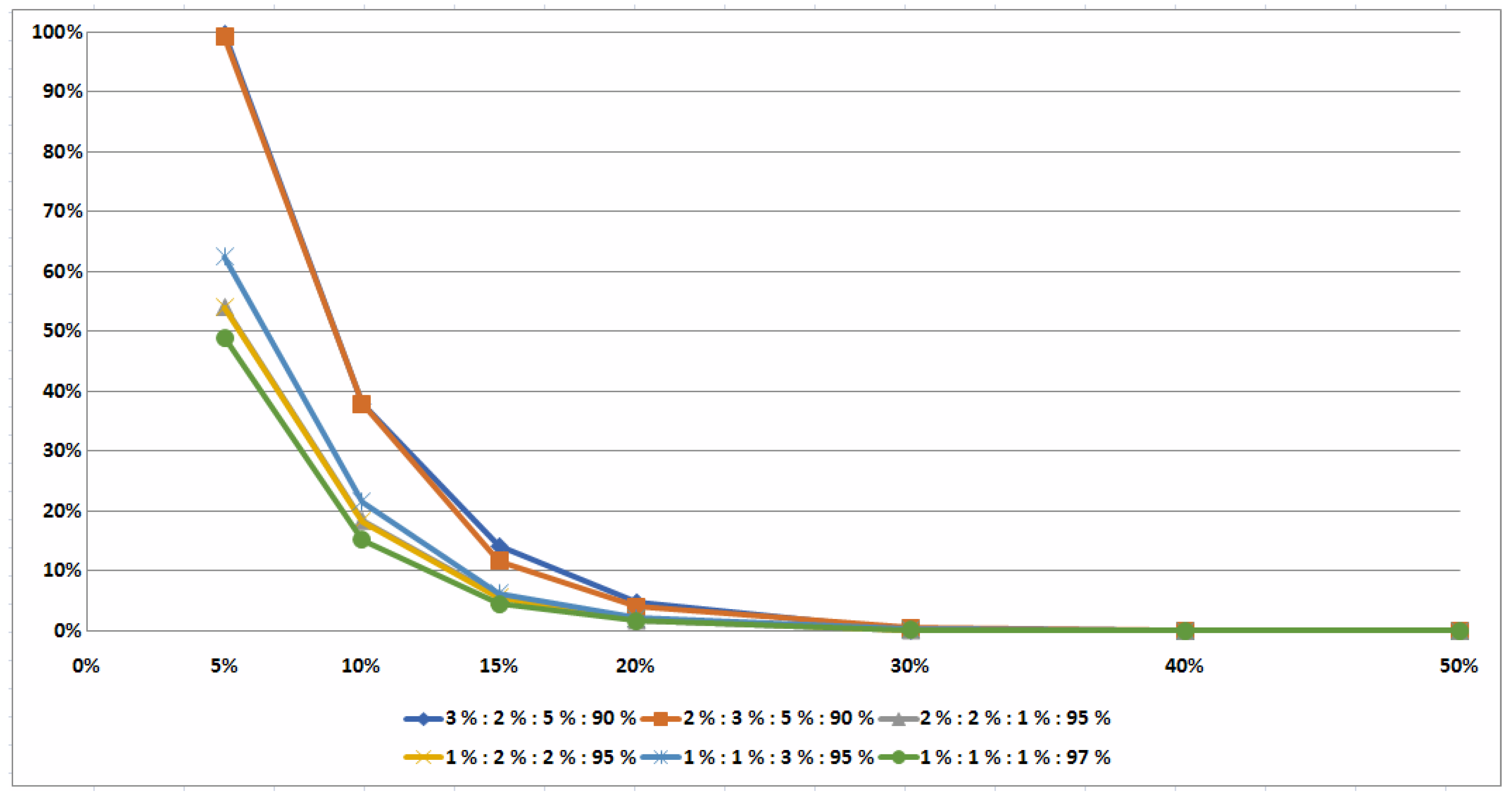
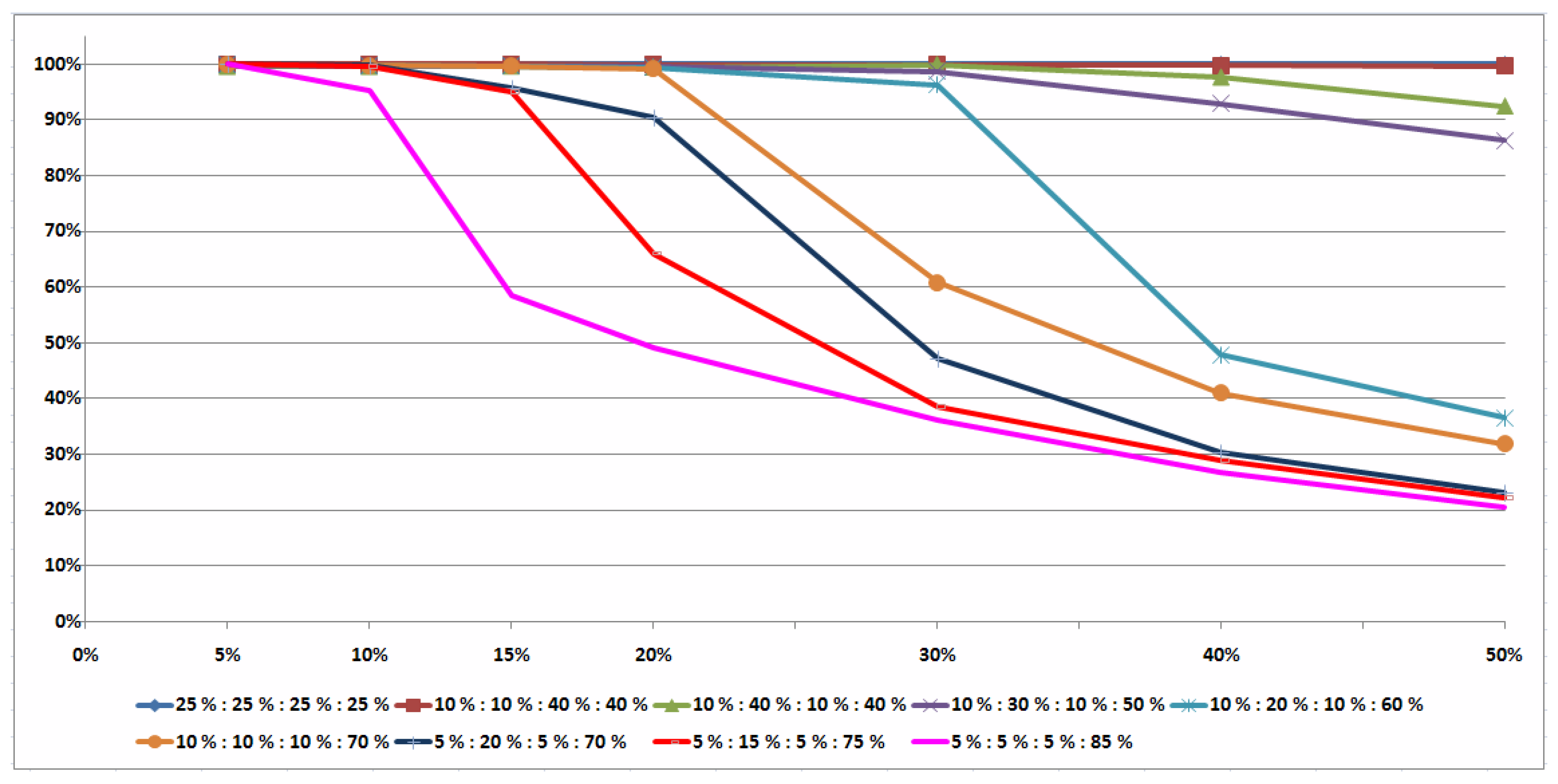
Average percentages of the instances which were optimally solved ($Opt$) are presented in Figure 1 for classes 1–9 of the tested instances and in Figure 2 for classes 10–15 of the hard-tested instances.

Figure 1. Average percentages of the instances presented in Table A1, Table A2, Table A3, Table A4, Table A5, Table A6, Table A7, Table A8 and Table A9, which were optimally solved at the off-line phase of scheduling.

Figure 2. Average percentages of the instances presented in Table A10, Table A11, Table A12, Table A13, Table A14 and Table A15, which were optimally solved at the off-line phase of scheduling.

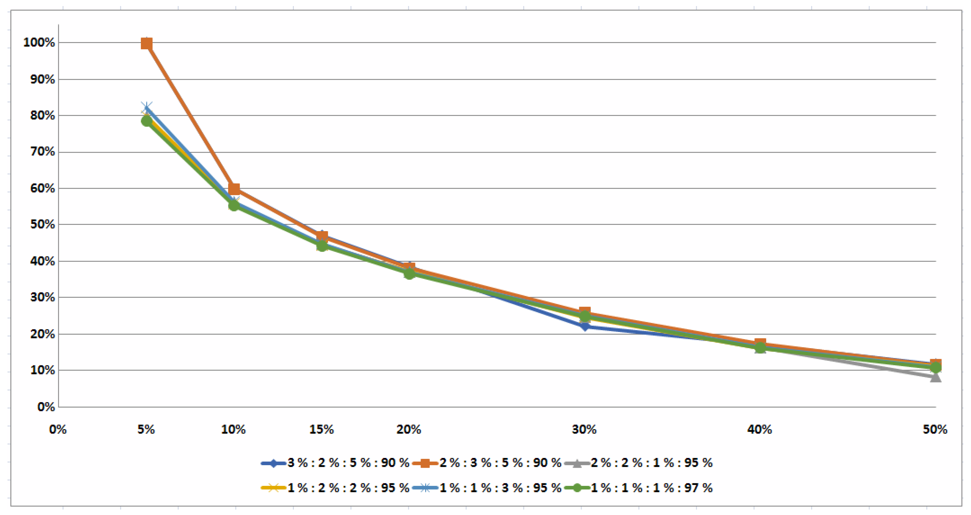
Percentages of the average values of the correct decisions ($SC$) made for determining optimal orders of the conflict jobs for classes 1–9 are presented in Figure 3. Most instances from these nine classes were optimally solved (Table 2). If the values of $\delta$ were no greater than $20\%$, i.e., $\delta \in \{5\%,10\%,15\%,20\%\}$, then more than $80\%$ of the tested instances were optimally solved in spite of the data uncertainty. If the value $\delta$ is increased, the percentage of the optimally solved instances decreased. If the value $\delta$ was equal to $50\%$, then $45\%$ of the tested instances was optimally solved.

Figure 3. Average percentages of the correct decisions made for constructing permutations of the conflict jobs for the instances presented in Table A1, Table A2, Table A3, Table A4, Table A5, Table A6, Table A7, Table A8, Table A9.

Table 2. Average percentage of the instances which were optimally solved.

$\mathit{\delta }\%$	5%	10%	15%	20%	30%	40%	50%	Average
Instances from Table A1, Table A2, Table A3, Table A4, Table A5, Table A6, Table A7, Table A8 and Table A9	99.93	98.48	88.93	80.66	63.97	50.18	44.10	75.18
Instances from Table A10, Table A11, Table A12, Table A13, Table A14 and Table A15	69.78	24.89	7.96	2.73	0.20	0.03	0.00	15.08

For all series of the hard instances presented in Table A10, Table A11, Table A12, Table A13, Table A14 and Table A15 (see the third line in Table 2), only a few instances were optimally solved. If $\delta =5\%$, then $70\%$ of the tested instances was optimally solved. If value $\delta$ belongs to the set $\{20\%,30\%,40\%,50\%\}$, then only $1\%$ of the tested instances was optimally solved. There were no hard-tested instances optimally solved for the value of $\delta =50\%$.

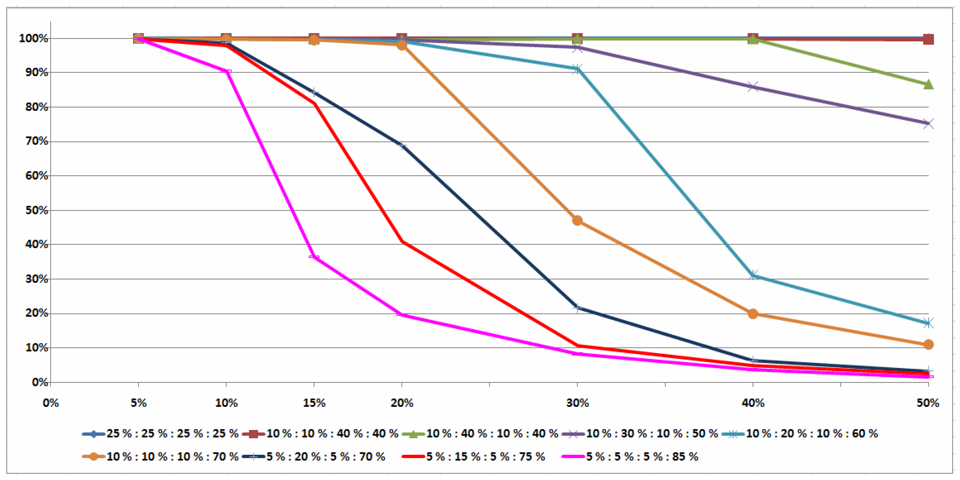
Percentages of the average values of the correct decisions made for determining optimal orders of the conflict jobs by Algorithm 2, Algorithm 3 and Algorithm 4 for the hard classes 10–15 of the tested instances are presented in Figure 4. Note that there is a correlation between values of $Opt$ and $SC$ presented in Figure 1 and Figure 3 for classes 1–9 of the tested instances and those presented in Figure 2 and Figure 4 for classes 10–15 of the hard-tested instances.

Figure 4. Average percentages of the correct decisions made for constructing permutations of the conflict jobs for the hard instances presented in Table A10, Table A11, Table A12, Table A13, Table A14 and Table A15.

8. Concluding Remarks and Future Works

The uncertain flow-shop scheduling problem $F2|l_{ij}\le p_{ij}\le u_{ij}|C_{max}$ and its generalization the job-shop problem $J2|l_{ij}\le p_{ij}\le u_{ij},n_i\le 2|C_{max}$ attract the attention of researchers since these problems are applicable in many real-life scheduling systems. The optimal scheduling decisions for these problems allow the plant to reduce the costs of productions due to a better utilization of the available machines and other resources. In Section 5, we proved several properties of the optimal pairs $({\pi }^{\prime },{\pi }^{″})$ of job permutations (Theorems 7–12). Using these properties, we derived Algorithms 1–4 for constructing optimal pairs $({\pi }^{\prime },{\pi }^{″})$ of job permutations or a small dominant set of schedules for the problem $J2|l_{ij}\le p_{ij}\le u_{ij},n_i\le 2|C_{max}$. If it is impossible to construct a single pair $({\pi }^{\prime },{\pi }^{″})$ of job permutations, which dominates all other pairs of job permutations for all possible scenarios T, then Algorithm 2 determines the partial strict order $A_{\prec }^{1,2}$ on the job set ${\mathcal{J}}_{1,2}$ (Algorithm 3) and the partial strict order $A_{\prec }^{2,1}$ on the job set ${\mathcal{J}}_{2,1}$ (Algorithm 4). The precedence digraphs $({\mathcal{J}}_{1,2},A_{\prec }^{1,2})$ and $({\mathcal{J}}_{2,1},A_{\prec }^{2,1})$ determine a minimal dominant set of schedules for the problem $J2|l_{ij}\le p_{ij}\le u_{ij},n_i\le 2|C_{max}$.

From the conducted extensive computational experiments, it follows that pairs of job permutations constructed using Algorithm 2 are close to the optimal pairs of job permutations, which may be determined after completing all jobs $\mathcal{J}$ when factual operation durations become known. We tested 15 classes of the randomly generated instances $J2|l_{ij}\le p_{ij}\le u_{ij},n_i\le 2|C_{max}$. Most instances from tested classes 1–9 were optimally solved at the off-line phase of scheduling. If the values of $\delta$ were no greater than $20\%$, i.e., $\delta \in \{5\%,10\%,15\%,20\%\}$, then more than $80\%$ of the tested instances was optimally solved in spite of the uncertainty of the input data. If $\delta =50\%$, then $45\%$ of the tested instances was optimally solved. However, less than $5\%$ of the instances with $\delta \ge 20\%$ from hard classes 10–15 were optimally solved at the off-line phase of scheduling (Figure 2). There were no tested hard instances optimally solved for the value $\delta =50\%$.

In future research, the on-line phase of scheduling will be studied for the problem $J2|l_{ij}\le p_{ij}\le u_{ij},n_i\le 2|C_{max}$. To this end, it will be useful to find sufficient conditions for existing a dominant pair of job permutations at the on-line phase of scheduling. The additional information on the factual value of the job duration becomes available once the processing of the job on the corresponding machine is completed. Using this additional information, a scheduler can determine a smaller dominant set DS of schedules, which is based on sufficient conditions for schedule dominance. The smaller DS enables a scheduler to quickly make an on-line scheduling decision whenever additional information on processing the job becomes available. To solve the problem $J2|l_{ij}\le p_{ij}\le u_{ij},n_i\le 2|C_{max}$ at the on-line phase, a scheduler needs to use fast (better polynomial) algorithms. The investigation of the on-line phase of scheduling for the uncertain job-shop problem is under development.

We suggest to investigate properties of the optimality box and optimality region for a pair $({\pi }^{\prime },{\pi }^{″})$ of the job permutations and to develop algorithms for constructing a pair $({\pi }^{\prime },{\pi }^{″})$ of the job permutations that have the largest optimality box (or the largest optimality region). We also suggest to apply the stability approach for solving the uncertain flow-shop and job-shop scheduling problems with $\left|\mathcal{M}\right|>2$ available machines.

Appendix A.1. Proof of Lemma 2

We choose an arbitrary vector p in the set T, $p\in T$, and show that set $<S_{1,2}^{\prime },S_{2,1}>$ contains at least one optimal pair of job permutations for the problem $J2|p,n_i\le 2|C_{max}$ with scenario $p\in T$.

Let $({\pi }^{*},{\pi }^{**})=(({\pi }_{1,2}^{*},{\pi }_1,{\pi }_{2,1}^{*}),({\pi }_{2,1}^{*},{\pi }_2,{\pi }_{1,2}^{*}))$ be a Jackson’s pair of job permutations for the problem $J2|p,n_i\le 2|C_{max}$ with scenario $p\in T$, i.e., $C_{max}({\pi }^{*},{\pi }^{**})=C_{max}$. Without loss of generality, one can assume that jobs in both permutations ${\pi }_1$ and ${\pi }_2$ are ordered in increasing order of their indexes. It is clear that ${\pi }_{2,1}^{*}\in S_{2,1}$. If inclusion ${\pi }_{1,2}^{*}\in S_{1,2}^{\prime }$ holds as well, then $({\pi }^{*},{\pi }^{**})\in <S_{1,2}^{\prime },S_{2,1}>$ and set $<S_{1,2}^{\prime },S_{2,1}>$ contains an optimal pair of job permutations for the problem $J2|p,n_i\le 2|C_{max}$ with scenario $p\in T$. We now assume that ${\pi }_{1,2}^{*}\notin S_{1,2}^{\prime }$. The set $S_{1,2}^{\prime }$ contains at least one optimal permutation for the problem $F2|p_{1,2}|C_{max}$ with job set ${\mathcal{J}}_{1,2}$ and scenario $p_{1,2}$ (the components of vector $p_{1,2}$ are equal to the corresponding components of vector p). We denote this permutation as ${\pi }_{1,2}^{\prime }$. Remember that permutation ${\pi }_{1,2}^{\prime }$ may be not a Johnson’s permutation for the problem $F2|p_{1,2}|C_{max}$ with job set ${\mathcal{J}}_{1,2}$ and scenario $p_{1,2}$. We consider a pair of job permutations $({\pi }^{\prime },{\pi }^{**})=(({\pi }_{1,2}^{\prime },{\pi }_1,{\pi }_{2,1}^{*}),$$({\pi }_{2,1}^{*},{\pi }_2,{\pi }_{1,2}^{\prime }))\in <S_{1,2}^{\prime },S_{2,1}>$ and show that equality $C_{max}({\pi }^{\prime },{\pi }^{**})=C_{max}$ holds. We consider the following two possible cases.

(j)$C_{max}({\pi }^{\prime },{\pi }^{**})=c_1\left({\pi }^{\prime }\right)$.

If equality $c_1\left({\pi }^{\prime }\right)={\sum }_{J_i\in {\mathcal{J}}_{1,2}\cup {\mathcal{J}}_{2,1}\cup {\mathcal{J}}_1}{p}_{i1}$ holds, then $c_1\left({\pi }^{\prime }\right)\le c_1\left({\pi }^{*}\right)$.

We now assume that inequality $c_1\left({\pi }^{\prime }\right)>{\sum }_{J_i\in {\mathcal{J}}_{1,2}\cup {\mathcal{J}}_{2,1}\cup {\mathcal{J}}_1}{p}_{i1}$ holds. Then, machine $M_1$ has an idle time. As it is mentioned in the proof of Theorem 7, an idle time for machine $M_1$ is only possible if some job $J_j$ from the set ${\mathcal{J}}_{2,1}$ is processed on machine $M_2$ at the time moment $t_2$ when job $J_j$ could be processed on machine $M_1$. Thus, the value of $c_1\left({\pi }^{\prime }\right)$ is equal to the makespan $C_{max}\left({\pi }_{2,1}^{*}\right)$ for the problem $F2|p_{2,1}|C_{max}$ with job set ${\mathcal{J}}_{2,1}$ and scenario $p_{2,1}$ (the components of vector $p_{2,1}$ are equal to the corresponding components of vector p). As jobs from the set ${\mathcal{J}}_{2,1}$ are processed as in the permutation ${\pi }_{2,1}^{*}$, which is a Johnson’s permutation, the value of $c_1\left({\pi }^{\prime }\right)$ cannot be reduced and so $c_1\left({\pi }^{\prime }\right)\le c_1\left({\pi }^{*}\right)$. We obtain the following relations: $C_{max}({\pi }^{\prime },{\pi }^{**})=c_1\left({\pi }^{\prime }\right)\le c_1\left({\pi }^{*}\right)\le max\{c_1\left({\pi }^{*}\right),c_2\left({\pi }^{**}\right)\}=C_{max}({\pi }^{*},{\pi }^{**})=C_{max}.$ Thus, equality $C_{max}({\pi }^{\prime },{\pi }^{**})=C_{max}$ holds.

(jj)$C_{max}({\pi }^{\prime },{\pi }^{**})=c_2\left({\pi }^{**}\right)$.

Similarly to case (j), we obtain the following equality:

$$c_2\left({\pi }^{**}\right)=max\{\sum _{J_i\in {\mathcal{J}}_{1,2}\cup {\mathcal{J}}_{2,1}\cup {\mathcal{J}}_2}{p}_{i2},C_{max}\left({\pi }_{1,2}^{\prime }\right)\},$$

where $C_{max}\left({\pi }_{1,2}^{\prime }\right)$ is the makespan for the problem $F2|p_{1,2}|C_{max}$ with job set ${\mathcal{J}}_{1,2}$ and vector $p_{1,2}$ of the job durations (it is assumed that ${\pi }_{1,2}^{\prime }$ is an optimal permutation for this problem). Thus, the value of $c_2\left({\pi }^{**}\right)$ cannot be reduced and equality $C_{max}({\pi }^{\prime },{\pi }^{**})=C_{max}$ holds.

In both considered cases, the pair of job permutations $({\pi }^{\prime },{\pi }^{**})$ is an optimal schedule for the problem $J2|p,n_i\le 2|C_{max}$ with scenario $p\in T$. Therefore, an optimal pair of job permutations for the problem $J2|p,n_i\le 2|C_{max}$ with scenario $p\in T$ belongs to the set $<S_{1,2}^{\prime },S_{2,1}>$. As vector p is an arbitrary vector in set T, the set $<S_{1,2}^{\prime },S_{2,1}>$ contains an optimal pair of job permutations for each scenario from set T. Due to Definition 4, the set $<S_{1,2}^{\prime },S_{2,1}>$ is a dominant set of schedules for the problem $J2|l_{ij}\le p_{ij}\le u_{ij},n_i\le 2|C_{max}$ with job set $\mathcal{J}$.

Appendix A.2. Proof of Theorem 8

We consider an arbitrary vector $p\in T$ of the job durations from set T and relevant vectors $p_{1,2}$ and $p_{2,1}$ of the durations of jobs from set ${\mathcal{J}}_{1,2}$ and set ${\mathcal{J}}_{2,1}$, respectively. Set $S_{1,2}^{\prime }$ contains an optimal permutation ${\pi }_{1,2}^{\prime }$ for the problem $F2|p_{1,2}|C_{max}$ with job set ${\mathcal{J}}_{1,2}$ and with vector $p_{1,2}$ of the job durations. Set $S_{2,1}^{\prime }$ contains an optimal permutation ${\pi }_{2,1}^{\prime }$ for the problem $F2|p_{2,1}|C_{max}$ with job set ${\mathcal{J}}_{2,1}$ and with vector $p_{2,1}$ of the job durations. We next show that the pair of job permutations $({\pi }^{\prime },{\pi }^{″})=(({\pi }_{1,2}^{\prime },{\pi }_1,{\pi }_{2,1}^{\prime }),$$({\pi }_{2,1}^{\prime },{\pi }_2,{\pi }_{1,2}^{\prime }))$ is an optimal pair of job permutations for the problem $J2|p,n_i\le 2|C_{max}$ with scenario $p\in T$ (the jobs in permutations ${\pi }_1$ and ${\pi }_2$ are ordered in increasing order of their indexes). From the proofs of Lemmas 2 and 3, we obtain the value of $C_{max}({\pi }^{\prime },{\pi }^{″})=max\{c_1\left({\pi }^{\prime }\right),c_2\left({\pi }^{″}\right)\}$

$$=max\{max\{\sum _{J_i\in {\mathcal{J}}_{1,2}\cup {\mathcal{J}}_{2,1}\cup {\mathcal{J}}_1}{p}_{i1},C_{max}({\pi }_{2,1}^{\prime })\},max\{\sum _{J_i\in {\mathcal{J}}_{1,2}\cup {\mathcal{J}}_{2,1}\cup {\mathcal{J}}_2}{p}_{i2},C_{max}({\pi }_{1,2}^{\prime })\}\},$$

which cannot be reduced. Therefore, $C_{max}({\pi }^{\prime },{\pi }^{″})=C_{max}$. An optimal pair of job permutations for the problem $J2|p,n_i\le 2|C_{max}$ with vector $p\in T$ of the job durations belongs to the set $<S_{1,2}^{\prime },S_{2,1}^{\prime }>$. As vector p is arbitrary in set T, the set $<S_{1,2}^{\prime },S_{2,1}^{\prime }>$ contains an optimal pair of job permutations for all vectors from set T. Due to Definition 4, the set $<S_{1,2}^{\prime },S_{2,1}^{\prime }>\subseteq S$ is a dominant set of schedules for the problem $J2|l_{ij}\le p_{ij}\le u_{ij},n_i\le 2|C_{max}$ with job set $\mathcal{J}$.

Appendix A.3. Proof of Theorem 9

We consider an arbitrary scenario $p\in T$. Due to Definition 1, the permutation ${\pi }_{1,2}$ is a Johnson’s permutation for the problem $F2|p_{1,2}|C_{max}$ with job set ${\mathcal{J}}_{1,2}$ and scenario $p_{1,2}$ (the components of this vector are equal to the corresponding components of vector p). Due to Definition 4, the singleton $\left\{({\pi }_{1,2},{\pi }_{1,2})\right\}$ is a minimal dominant set of schedules for the problem $F2|l_{ij}\le p_{ij}\le u_{ij}|C_{max}$ with job set ${\mathcal{J}}_{1,2}$.

Similarly, the singleton $\left\{({\pi }_{2,1},{\pi }_{2,1})\right\}$ is a minimal dominant set of schedules for the problem $F2|l_{ij}\le p_{ij}\le u_{ij}|C_{max}$ with job set ${\mathcal{J}}_{2,1}$. We consider permutations ${\pi }_1$ and ${\pi }_2$ of the jobs ${\mathcal{J}}_1$ and ${\mathcal{J}}_2$, respectively (due to Remark 1, the jobs in permutations ${\pi }_1$ and ${\pi }_2$ are ordered in increasing order of their indexes). Due to Theorem 8, the pair of permutations $(({\pi }_{1,2},{\pi }_1,{\pi }_{2,1}),({\pi }_{1,2},{\pi }_2,{\pi }_{2,1}))$ is a single-element dominant set (DS(T)) for the problem $J2|l_{ij}\le p_{ij}\le u_{ij},n_i\le 2|C_{max}$ with job set $\mathcal{J}={\mathcal{J}}_1\cup {\mathcal{J}}_2\cup {\mathcal{J}}_{1,2}\cup {\mathcal{J}}_{2,1}$.

Appendix A.4. Proof of Corollary 6

In the proof of Theorem 9, it is shown that the pair of job permutations $(({\pi }_{1,2},{\pi }_1,{\pi }_{2,1}),$$({\pi }_{1,2},{\pi }_2,{\pi }_{2,1}))$ is a single-element dominant set of schedules for the problem $J2|l_{ij}\le p_{ij}\le u_{ij},n_i\le 2|C_{max}$ with job set $\mathcal{J}={\mathcal{J}}_1\cup {\mathcal{J}}_2\cup {\mathcal{J}}_{1,2}\cup {\mathcal{J}}_{2,1}$. We next show that the pair of permutations $(({\pi }_{1,2},{\pi }_1,{\pi }_{2,1}),({\pi }_{1,2},{\pi }_2,{\pi }_{2,1}))$ satisfies to Definition 1, i.e., this pair of permutations is a Jackson’s pair of job permutations for the problem $J2|l_{ij}\le p_{ij}\le u_{ij},n_i\le 2|C_{max}$ with job set $\mathcal{J}$ (the minimality condition is obvious). Indeed, due to conditions of Theorem 9, the permutation ${\pi }_{1,2}$ is a Johnson’s permutation for the problem $F2|l_{ij}\le p_{ij}\le u_{ij}|C_{max}$ with job set ${\mathcal{J}}_{1,2}$ and the permutation ${\pi }_{2,1}$ is a Johnson’s permutation for the problem $F2|l_{ij}\le p_{ij}\le u_{ij}|C_{max}$ with job set ${\mathcal{J}}_{2,1}$. Therefore, pair $(({\pi }_{1,2},{\pi }_1,{\pi }_{2,1}),({\pi }_{1,2},{\pi }_2,{\pi }_{2,1}))$ is a Jackson’s pair of permutations for the problem $J2|l_{ij}\le p_{ij}\le u_{ij},n_i\le 2|C_{max}$ with job set $\mathcal{J}$. Due to Definition 1, the pair of job permutations $(({\pi }_{1,2},{\pi }_1,{\pi }_{2,1}),({\pi }_{1,2},{\pi }_2,{\pi }_{2,1}))$ is a single-element J-solution for the problem $J2|l_{ij}\le p_{ij}\le u_{ij},n_i\le 2|C_{max}$ with job set $\mathcal{J}={\mathcal{J}}_1\cup {\mathcal{J}}_2\cup {\mathcal{J}}_{1,2}\cup {\mathcal{J}}_{2,1}$.

Appendix A.5. Proof of Theorem 12

We consider any fixed scenario $p\in T$ and a pair of job permutations $({\pi }^{\prime },{\pi }^{″})=((\pi ,{\pi }_1,{\pi }_{2,1}^{*}),({\pi }_{2,1}^{*},{\pi }_2,\pi ))\in S^{\prime }$, where ${\pi }_{2,1}^{*}\in S_{2,1}$ is a Johnson’s permutation of the jobs from the set ${\mathcal{J}}_{2,1}$ with vector $p_{2,1}$ of the job durations (components of this vector are equal to the corresponding components of vector p). We next show that this pair of job permutations $({\pi }^{\prime },{\pi }^{″})$ is optimal for the individual problem $J2|p,n_i\le 2|C_{max}$ with scenario p, i.e., $C_{max}({\pi }^{\prime },{\pi }^{″})=C_{max}$.

At time $t=0$, machine $M_1$ begins to process jobs from the permutation $\pi$ without idle times. We denote $t_1={\sum }_{i=1}^{k+r+1}{p}_{i1}.$ At time moment $t_1$, job $J_{k+r+1}$ is ready for processing on machine $M_2$. From the condition of Inequality (13) with $s=1$, it follows that, even if machine $M_2$ has an idle time before processing job $J_{k+r+1}$, machine $M_2$ is available for processing this job at time $t_1$. If in addition, the condition of Inequality (13) holds with $s\in \{2,3,\dots ,r\}$, then machine $M_2$ may also have idle times between processing jobs from the conflict set $\{J_{k+1},J_{k+2},\dots ,J_{k+r}\}.$ However, machine $M_2$ is available for processing job $J_{k+r+1}$ from the time moment $t_1={\sum }_{i=1}^{k+r+1}{p}_{i1}.$

In permutation $\pi$, jobs $J_{k+r+1},\dots ,J_{m_{1,2}}$ are arranged in Johnson’s order. Therefore, if machine $M_2$ has an idle time while processing these jobs, this idle time cannot be reduced.

Thus, the value of $c_2\left({\pi }^{″}\right)$ cannot be reduced by changing the order of jobs from the conflict set. Note that an idle time for machine $M_1$ is only possible between some jobs from the set ${\mathcal{J}}_{2,1}$. Since the permutation ${\pi }_{2,1}^{*}$ is a Johnson’s permutation of the jobs from set ${\mathcal{J}}_{2,1}$ with scenario $p_{2,1}$, the value of $c_1\left({\pi }^{\prime }\right)$ cannot be reduced. Thus, we obtain $C_{max}({\pi }^{\prime },{\pi }^{″})=max\{c_1\left({\pi }^{\prime }\right),c_2\left({\pi }^{″}\right)\}=C_{max}$ and the pair of permutations $({\pi }^{\prime },{\pi }^{″})=((\pi ,{\pi }_1,{\pi }_{2,1}^{*}),({\pi }_{2,1}^{*},{\pi }_2,\pi ))\in S^{\prime }$ is optimal for the problem $J2|p,n_i\le 2|C_{max}$ with scenario $p\in T$. As the vector p is an arbitrary vector in the set T, set $S^{\prime }$ contains an optimal pair of job permutations for each vector from the set T. Due to Definition 4, set $S^{\prime }$ is a dominant set of schedules for the problem $J2|l_{ij}\le p_{ij}\le u_{ij},n_i\le 2|C_{max}$ with job set $\mathcal{J}$.

References

- Pinedo, M. Scheduling: Theory, Algorithms, and Systems; Prentice-Hall: Englewood Cliffs, NJ, USA, 2002. [Google Scholar]
- Elmaghraby, S.; Thoney, K.A. Two-machine flowshop problem with arbitrary processing time distributions. IIE Trans. 2000, 31, 467–477. [Google Scholar] [CrossRef]
- Kamburowski, J. Stochastically minimizing the makespan in two-machine flow shops without blocking. Eur. J. Oper. Res. 1999, 112, 304–309. [Google Scholar] [CrossRef]
- Ku, P.S.; Niu, S.C. On Johnson’s two-machine flow-shop with random processing times. Oper. Res. 1986, 34, 130–136. [Google Scholar] [CrossRef]
- Allahverdi, A. Stochastically minimizing total flowtime in flowshops with no waiting space. Eur. J. Oper. Res. 1999, 113, 101–112. [Google Scholar] [CrossRef]
- Allahverdi, A.; Mittenthal, J. Two-machine ordered flowshop scheduling under random breakdowns. Math. Comput. Model. 1999, 20, 9–17. [Google Scholar] [CrossRef]
- Portougal, V.; Trietsch, D. Johnson’s problem with stochastic processing times and optimal service level. Eur. J. Oper. Res. 2006, 169, 751–760. [Google Scholar] [CrossRef]
- Daniels, R.L.; Kouvelis, P. Robust scheduling to hedge against processing time uncertainty in single stage production. Manag. Sci. 1995, 41, 363–376. [Google Scholar] [CrossRef]
- Sabuncuoglu, I.; Goren, S. Hedging production schedules against uncertainty in manufacturing environment with a review of robustness and stability research. Int. J. Comput. Integr. Manuf. 2009, 22, 138–157. [Google Scholar] [CrossRef]
- Sotskov, Y.N.; Werner, F. Sequencing and Scheduling with Inaccurate Data; Nova Science Publishers: Hauppauge, NY, USA, 2014. [Google Scholar]
- Pereira, J. The robust (minmax regret) single machine scheduling with interval processing times and total weighted completion time objective. Comput. Oper. Res. 2016, 66, 141–152. [Google Scholar] [CrossRef]
- Kasperski, A.; Zielinski, P. A 2-approximation algorithm for interval data minmax regret sequencing problems with total flow time criterion. Oper. Res. Lett. 2008, 36, 343–344. [Google Scholar] [CrossRef]
- Wu, Z.; Yu, S.; Li, T. A meta-model-based multi-objective evolutionary approach to robust job shop scheduling. Mathematics 2019, 7, 529. [Google Scholar] [CrossRef]
- Grabot, B.; Geneste, L. Dispatching rules in scheduling: A fuzzy approach. Int. J. Prod. Res. 1994, 32, 903–915. [Google Scholar] [CrossRef]
- Özelkan, E.C.; Duckstein, L. Optimal fuzzy counterparts of scheduling rules. Eur. J. Oper. Res. 1999, 113, 593–609. [Google Scholar] [CrossRef]
- Kasperski, A.; Zielinski, P. Possibilistic minmax regret sequencing problems with fuzzy parameteres. IEEE Trans. Fuzzy Syst. 2011, 19, 1072–1082. [Google Scholar] [CrossRef]
- Lai, T.-C.; Sotskov, Y.N.; Sotskova, N.Y.; Werner, F. Optimal makespan scheduling with given bounds of processing times. Math. Comput. Model. 1997, 26, 67–86. [Google Scholar]
- Lai, T.-C.; Sotskov, Y.N. Sequencing with uncertain numerical data for makespan minimization. J. Oper. Res. Soc. 1999, 50, 230–243. [Google Scholar] [CrossRef]
- Lai, T.-C.; Sotskov, Y.N.; Sotskova, N.Y.; Werner, F. Mean flow time minimization with given bounds of processing times. Eur. J. Oper. Res. 2004, 159, 558–573. [Google Scholar] [CrossRef]
- Sotskov, Y.N.; Egorova, N.M.; Lai, T.-C. Minimizing total weighted flow time of a set of jobs with interval processing times. Math. Comput. Model. 2009, 50, 556–573. [Google Scholar] [CrossRef]
- Cheng, T.C.E.; Shakhlevich, N.V. Proportionate flow shop with controllable processing times. J. Sched. 1999, 27, 253–265. [Google Scholar] [CrossRef]
- Cheng, T.C.E.; Kovalyov, M.Y.; Shakhlevich, N.V. Scheduling with controllable release dates and processing times: Makespan minimization. Eur. J. Oper. Res. 2006, 175, 751–768. [Google Scholar] [CrossRef]
- Jansen, K.; Mastrolilli, M.; Solis-Oba, R. Approximation schemes for job shop scheduling problems with controllable processing times. Eur. J. Oper. Res. 2005, 167, 297–319. [Google Scholar] [CrossRef]
- Graham, R.L.; Lawler, E.L.; Lenstra, J.K.; Rinnoy Kan, A.H.G. Optimization and approximation in deterministic sequencing and scheduling. Ann. Discret. Appl. Math. 1979, 5, 287–326. [Google Scholar]
- Brucker, P. Scheduling Algorithms; Springer: Berlin, Germany, 1995. [Google Scholar]
- Tanaev, V.S.; Sotskov, Y.N.; Strusevich, V.A. Scheduling Theory: Multi-Stage Systems; Kluwer Academic Publishers: Dordrecht, The Netherlands, 1994. [Google Scholar]
- Jackson, J.R. An extension of Johnson’s results on job lot scheduling. Nav. Res. Logist. Q. 1956, 3, 201–203. [Google Scholar] [CrossRef]
- Johnson, S.M. Optimal two and three stage production schedules with set up times included. Nav. Res. Logist. Q. 1954, 1, 61–68. [Google Scholar] [CrossRef]
- Allahverdi, A.; Sotskov, Y.N. Two-machine flowshop minimum-lenght scheduling problem with random and bounded processing times. Int. Trans. Oper. Res. 2003, 10, 65–76. [Google Scholar] [CrossRef]
- Matsveichuk, N.M.; Sotskov, Y.N. A stability approach to two-stage scheduling problems with uncertain processing times In Sequencing and Scheduling with Inaccurate Data; Sotskov, Y.N., Werner, F., Eds.; Nova Science Publishers: Hauppauge, NY, USA, 2014; pp. 377–407. [Google Scholar]
- Shafranski, Y.M. On the existence of globally optimal schedules for the Bellman-Johnson problem for two machines under uncertainty. Informatika 2009, 3, 100–110. (In Russian) [Google Scholar]
- Lai, T.-C.; Sotskov, Y.N.; Egorova, N.G.; Werner, F. The optimality box in uncertain data for minimising the sum of the weighted job completion times. Int. J. Prod. Res. 2018, 56, 6336–6362. [Google Scholar] [CrossRef]
- Sotskov, Y.N.; Egorova, N.G. Single machine scheduling problem with interval processing times and total completion time objective. Algorithms 2018, 11, 66. [Google Scholar] [CrossRef]
- Sotskov, Y.N.; Lai, T.-C. Minimizing total weighted flow time under uncertainty using dominance and a stability box. Comput. Oper. Res. 2012, 39, 1271–1289. [Google Scholar] [CrossRef]
- Sotskov, Y.N.; Egorova, N.G. Minimizing total flow time under uncertainty using optimality and stability boxes. In Sequencing and Scheduling with Inaccurate Data; Sotskov, Y.N., Werner, F., Eds.; Nova Science Publishers: Hauppauge, NY, USA, 2014; pp. 345–376. [Google Scholar]
- Matsveichuk, N.M.; Sotskov, Y.N.; Egorova, N.G.; Lai, T.-C. Schedule execution for two-machine flow-shop with interval processing times. Math. Comput. Model. 2009, 49, 991–1011. [Google Scholar] [CrossRef]
- Sotskov, Y.N.; Allahverdi, A.; Lai, T.-C. Flowshop scheduling problem to minimize total completion time with random and bounded processing times. J. Oper. Res. Soc. 2004, 55, 277–286. [Google Scholar] [CrossRef]
- Allahverdi, A.; Aldowaisan, T.; Sotskov, Y.N. Two-machine flowshop scheduling problem to minimize makespan or total completion time with random and bounded setup times. Int. J. Math. Math. Sci. 2003, 39, 2475–2486. [Google Scholar] [CrossRef]
- Kouvelis, P.; Yu, G. Robust Discrete Optimization and Its Application; Kluwer Academic Publishers: Boston, MA, USA, 1997. [Google Scholar]
- Kouvelis, P.; Daniels, R.L.; Vairaktarakis, G. Robust scheduling of a two-machine flow shop with uncertain processing times. IEEE Trans. 2011, 32, 421–432. [Google Scholar] [CrossRef]
- Ng, C.T.; Matsveichuk, N.M.; Sotskov, Y.N.; Cheng, T.C.E. Two-machine flow-shop minimum-length scheduling with interval processing times. Asia-Pac. J. Oper. Res. 2009, 26, 1–20. [Google Scholar] [CrossRef]
- Matsveichuk, N.M.; Sotskov, Y.N.; Werner, F. The dominance digraph as a solution to the two-machine flow-shop problem with interval processing times. Optimization 2011, 60, 1493–1517. [Google Scholar] [CrossRef]
© 2019 by the authors. Licensee MDPI, Basel, Switzerland. This article is an open access article distributed under the terms and conditions of the Creative Commons Attribution (CC BY) license (http://creativecommons.org/licenses/by/4.0/).