A Generalized MILP Formulation for the Period-Aggregated Resource Leveling Problem with Variable Job Duration

Abstract

We study a resource leveling problem with variable job duration. The considered problem includes both scheduling and resource management decisions. The planning horizon is fixed and separated into a set of time periods of equal length. There are several types of resources and their amount varies from one period to another. There is a set of jobs. For each job, a fixed volume of work has to be completed without any preemption while using different resources. If necessary, extra resources can be used at additional costs during each time period. The optimization goal is to minimize the total overload costs required for the execution of all jobs by the given deadline. The decision variables specify the starting time of each job, the duration of the job and the resource amount assigned to the job during each period (it may vary over periods). We propose a new generalized mathematical formulation for this optimization problem. The formulation is compared with existing approaches from the literature. Theoretical study and computational experiments show that our approach provides more flexible resource allocation resulting in better final solutions.

1. Introduction

In the field of operations research, project management remains a topic of intensive research from various angles such as scheduling and resource allocation. For both cases, there exist such well-known formulations as a resource-constrained project scheduling problem (RCPSP) and a resource leveling problem (RLP). The former aims to minimize the completion time of the set of jobs with given precedence relations and the set of limited required resources. The latter deals with resource allocation with the objective to minimize the cost of resource usage. Both problems were proved to be NP-hard (see [1] for RCPSP and [2] for the resource leveling problem). To respond to practical requirements, these basic models undergo numerous modifications. For example, the model that optimizes the distribution of man hours for workforce or throughput on a production line was presented by Neubert and Savino [3].

In this paper, we focus on the resource leveling problem with several practical enhancements. However, we also refer to RCPSP modeling techniques and approaches that are used for the RLP and applicable to our case. The RLP was actively studied from both the theoretical and practical sides. In the paper of Rieck and Zimmermann [4] three basic objective function types from the existing literature were presented with properties and existing solution approaches. The first objective function type was described as a total amount of variations in resource utilization within the project duration. The second case arises when available resource utilization is exceeded; it is total (squared) overload cost. The authors also presented a total adjustment cost function, which is formed by costs arising from increasing and decreasing resource utilization. In all cases, the planning horizon was fixed with the reference that for mid-term planning usually there is a determined project deadline. There are some papers involving multi-criteria optimization techniques with attention to both project duration and resource utilization. However, RLP with a fixed deadline and the objective functions that were presented above still attracts attention: The majority of the following literature references are focused on this formulation.

From the practical side, these RLP types are found in a wide range of industries, especially in construction. For these particular cases, researchers apply different heuristics to provide good solutions. An overview of existing RLP heuristic techniques was prepared by Christodoulou et al. [5]. We can point out recent results with references to industrial problems. For example, a meta-heuristic genetic algorithm was applied to RLP based on a construction project in the paper of Selvam and Tadepalli [6]. Simulated annealing was also tested in the construction area by Piryonesi et al. [7]. Li et al. [8] implemented a genetic algorithm for the RLP with uncertain activity durations and possible overlapping. Construction area and project management usually include discrete resources such as equipment, machines, materials or manpower. Cherkaoui et al. [9] studied a tactical level of construction and large-scale engineering planning. To achieve robust tactical planning and resource allocation, they created a proactive approach providing lower variations in project costs in case of resource capacity uncertain data. The problem was denoted as rough cut capacity planning (RCCP), but it is also similar to the classical RLP with several practical changes. The same notation was also used by Baydoun et al. [10].

There is another point that inspires us to study and develop RLP solution methods. Energy is the main continuous resource, and the energy management problem becomes more and more crucial for any industry. According to this, the scheduling of operations with attention to careful energy consumption remains actual. Artigues et al. [11] considered the industrial case of the energy scheduling problem for a pipe-manufacturing plant. The goal was to minimize the electricity bill, which was raised by penalties for power overrun. The two-step solution approach was proposed with a constraint programming assignment and sequencing part and an MILP scheduling and energy part. Many industrial management problems can be represented as RLP, especially if the parameters are defined and well formalized. Sometimes the energy is not the main resource. For example, for computer embedded systems it can be CPU power, and for data transfer networks it is channel capacity. An example of an optimization problem from the space industry could be found in the paper of Capelle et al. [12]. In this practical study, the goal was to maximize a data transfer from satellites to a network of optical ground stations. While we see that this formulation is closer to an assignment problem, further research may fit in RLP formulation with satellite data buffer capacity, energy, and data transfer limits.

For the resource leveling problem, the case with variable job duration was considered by Hans, who proposed a branch and cut algorithm [13]; furthermore, Kis developed an improved branching scheme [14]. In these models, the precedence relations are defined on periods and job duration depends on the resources allocated to each job. The resource consumption is calculated in an aggregated way for each period. The concept of variable job duration has also been modeled in the following studies (see [4,15]) but with the objective of makespan minimization or balanced profile usage. Bianco et al. [16] also considered the resource leveling problem and proposed a lower bound based on Lagrangian relaxation, and a branch and bound algorithm for the suggested model. The resource leveling model with the overload cost and overlapping of jobs with precedence relations was presented by Baydoun et al. [10] with a focus on different overlapping rules such as overlapping after implementation of some essential predecessor part.

We follow these ideas and study the generalization of models presented by Baydoun et al. [10] and Bianco et al. [16]. The goal is to minimize overload cost when an extra resource amount is required beyond the available limit. In contrast to these studies, we consider a more flexible resource distribution. The main difference could be presented in the following way. In these papers, there is one decision variable (denoted as assigned workload [10] or the fraction [16] of activity in a period) describing the progress made by a given job in a given period, and it defines the requirement for each resource type. In our case, we enrich the model to make the allocation of resources per period independently with additional decision variables.

For example, suppose there is one job j which requires overall one unit of resource $r_1$ and two units of resource $r_2$. In the models considered by [10,16] the solution defines only job fractions (these models are denoted as ’aggregate fraction’ in the following). Suppose in the solution the job is implemented in two time periods with equal fractions in both periods (50%/50%). Then according to the models in the first period, we involve 0.5 units of resource $r_1$ and 1 unit of resource $r_2$, and the same in the second period. The involved resource amount equals the multiplication of this decision variable and a resource amount required to carry out the job (fixed input parameter). So there exists a constant ratio between the involved renewable resource amount (or efforts made by different resources) for a given job in all periods. We point out that particular fraction values are not important. With any fraction of the job j in any period, there will be the same ratio 0.5 between the involved resources (caused by the total required amount ratio of resource $r_1$ to resource $r_2$). According to our model, it is possible to make a more flexible allocation without any fixed relations between the resources involved to complete the job in some period. For example, it is possible to involve 0.75 units of $r_1$ and $0.5$ units of $r_2$ in the first period and the remaining 0.25 units of $r_1$ and $1.5$ units of $r_2$ in the second period. In this solution, resources are allocated with an independent ratio: 1.5 in the first period and 0.16 in the second period.

The main contribution of this paper is in the new generalized formulation for this type of resource leveling problem. We analyze the difference between this new generalized model and aggregated fraction models from the literature, with a comparison of performance and solution quality for the same instance set. Several particular formulations of this new approach were studied. We also study the case with discrete overloading of resources, which is compliant with human resources allocation. However, we do not consider job overlapping of predecessors and successors.

The rest of the paper is organized as follows. In Section 2 we present the new generalized formulation idea with several modeling implementations. We consider three different formulations of scheduling constraints and decision variables. After some experiments, we choose the binary step start/end formulation of variables for scheduling constraints. In Section 3 we describe a theoretical difference and relations between our generalized formulation and aggregated fraction and analyze the results of computational experiments. Section 4 presents the case of the discrete overload objective function and discrete resources. After, we make some concluding remarks.

2. Mathematical Model

2.1. Problem Parameters

The planning horizon is represented by the set of periods $T=\{1,\dots ,m\}$ with given length d, the last time period available defines the strict deadline for the execution of all the jobs. There is a set of jobs J and a set of resources R. For each job $j\in J$, some given work volume $W_{jr}$ must be executed with resource $r\in R$, while in each period $t\in T$ the available capacity $L_{rt}$ is known for each resource $r\in R$ is fixed. The allocation of an extra unit of resource capacity is subject to extra cost $e_r$. Work volume is the result of the multiplication of the assigned resource amount by the duration of its usage. Each job $j\in J$ has a given time window with lower $p_{min,jr}$ and upper $p_{max,jr}$ period for each resource $r\in R$. The pairs of predecessors and successors are defined in set P. The list of all parameters in our mathematical model is presented in

Table 1. Model nomenclature: Parameters notation.

Parameters
T	planning horizon, $T=\{1,\dots ,m\}$
d	period length
R	resources set
$L_{rt}$	availability of resource $r\in R$ in period $t\in T$
$e_r$	extra resource cost
J	jobs set
$W_{jr}$	job $j\in J$ work volume with resource $r\in R$
$p_{min,jr}$	job $j\in J$ minimal requirement per period in resource $r\in R$
$p_{max,jr}$	job $j\in J$ maximal requirement per period in resource $r\in R$
P	set of arcs in the given precedence graph

.

2.2. Generalized Model Description

For any kind of RLP, it is possible to separate the set of variables into two subsets, related to job scheduling and resource allocation. The subset of scheduling variables for discrete-time period models is well studied in project scheduling (starting from pioneer introduction of a 1-0 variable approach by Pritsker et al. [17]). Usually, it is a set of binaries that configure staring and ending periods. If we consider precedence relations and allow the successor to start we also use continuous duration variables responsible for the duration inside the period. We define binary variables responsible for the job starts and ends as $S_{jt}$ and $E_{jt}$, respectively. They may be used in several ways.

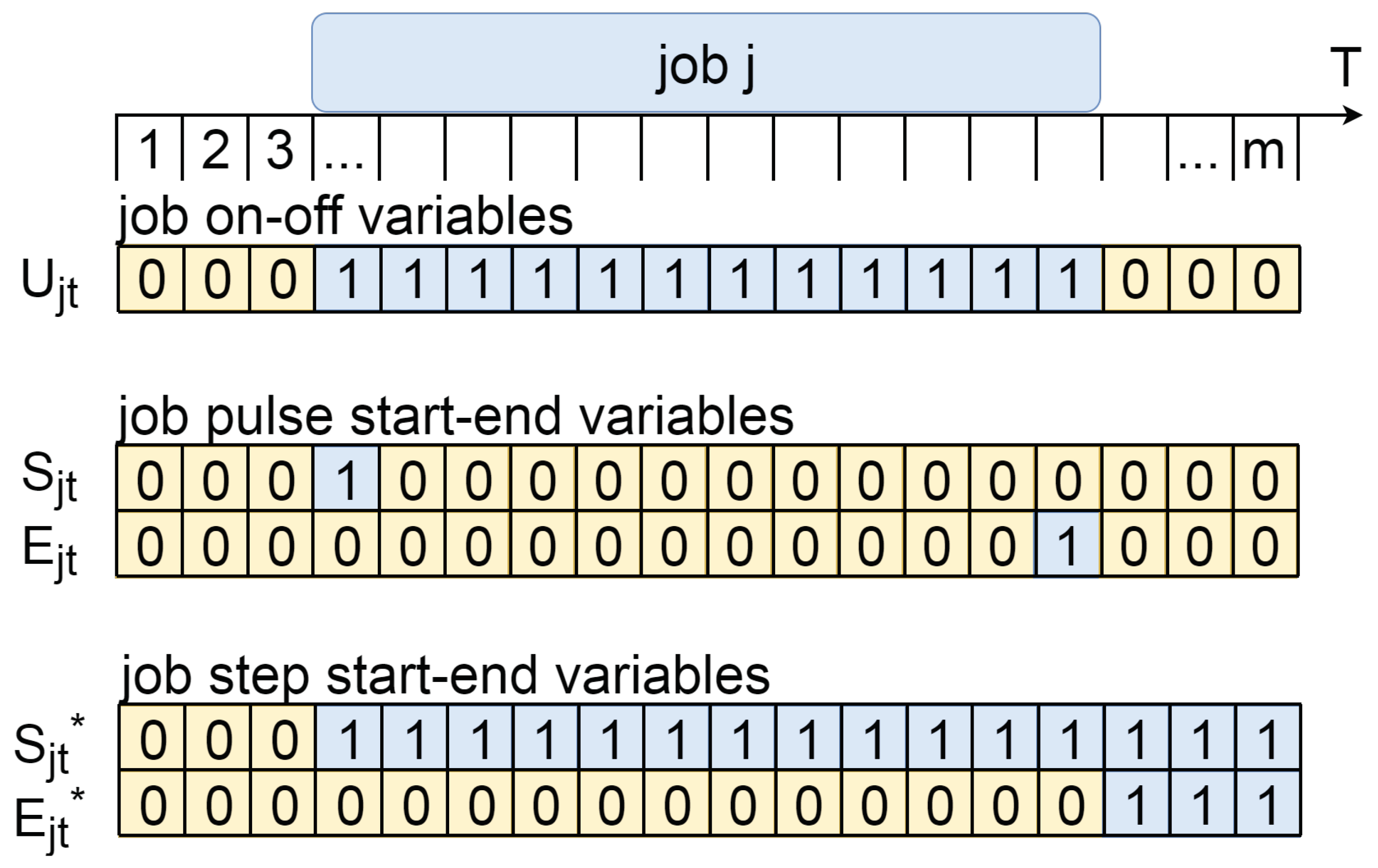
• As a step pointer, i.e., if job j starts at period t, then $\forall t_1<t$ $S_{j{t}_1}=0$ and $\forall t_2\ge t$ $S_{j{t}_2}=1$. In this case the same logic is implemented for $E_{jt}$, if a job ends at period t, than for $\forall t_1\le t$ $E_{jt}=0$ and $\forall t_2>t$ $E_{jt}=1$. To the best of our knowledge, in similar resource leveling models step pointer to job start and end periods is more common (for example, it was used by Baydoun et al. [10], Bianco et al. [16]).
• As an on–off (also referred as pulse) pointer, i.e., if job j starts at period t, then $\forall t_1\ne t$ $S_{j{t}_1}=0$ and $S_{jt}=1$ (the same logic for $E_{jt}$). This approach was considered by Tamas Kis and Marton Drotos, [18]. There is an alternative way, with an on–off function $U_{jt}$, where $U_{jt}=1$ if job j is implemented at period t, and $U_{jt}=0$ otherwise.

These approaches were also presented and compared in literature related to project scheduling, for example, see [19,20].

The second subset defines resource-allocation decision variables. We propose to generalize it and introduce separate fraction decision variables for each resource type instead of aggregated job fraction decision variables. In our case, these decision variables were defined as $c_{jrt}$. This approach makes an independent allocation of each resource type for every job. It leads to more flexible utilization of resources. However, it increases the size of the model and negatively affects performance, so it may require more computational resources to achieve a proofed optimal solution. We present a list of decision variable notations used in this paper in

Table 2. Model nomenclature: Decision variables notations.

Scheduling decision variables
$U_{jt}\in \{0,1\}$	on/off function : Equals 1 of job $j\in J$ is implemented in period $t\in T$, 0 otherwise
$S_{jt}\in \{0,1\}$	pulse start function : Equals 1 if job $j\in J$ starts in period $t\in T$, 0 otherwise
$E_{jt}\in \{0,1\}$	pulse end function : Equals 1 if job $j\in J$ ends in period $t\in T$, 0 otherwise
$S_{jt}^{*}\in \{0,1\}$	step start function : Equals 1 if job $j\in J$ starts in $\forall t_1\in T$, $t_1\le t$, 0 otherwise
$E_{jt}^{*}\in \{0,1\}$	step end function : Equals 1 if job $j\in J$ ends in $\forall t_1\in T$, $t_1<t$, 0 otherwise
$d_{jt}\in [0,d]$	duration of job $j\in J$ in period $t\in T$
Resource allocation decision variables
$c_{jrt}\in [0,d{p}_{max,jr}]$	work volume of job $j\in J$ with resource $r\in R$ in period $t\in T$
$o_{rt}\in [0,\infty )$	extra cost of resource $r\in R$ in period $t\in T$

.

In the next subsections we describe three different approaches to represent scheduling constraints with binary variables. A general description of each type is presented in Figure 1.

2.2.1. Scheduling Constraints: Job On–Off Formulation

This set of constraints is defined as job on–off implementation formulation, as we use one binary variable implying that the job is implemented inside some period or not. This definition of binaries in project scheduling problems is denoted as pulse or on–off in literature. So we use a variable $U_{jt}\in \{0,1\}$, $U_{jt}=1$ if job j is implemented in period t, $U_{jt}=0$ otherwise. Constraints (1) imply that no preemptions are allowed.

$$(t_2-t_1-1)\le \sum _{l=t_1+1}^{t_2-1}{U}_{il}+m(U_{j,t_1}+U_{j,t_2}-2),\forall t_1\in T,t_2\in T,t_1<t_2,\forall j\in J.$$

(1)

If the job is implemented in some period $t_1\in T$ and in some period $t_2\in T$, $t_1<t_2$, then it must be also implemented in any period $t_3\in T$, $t_1<t_3<t_2$. In other words, if for some job j there exists $t_1\in T$, $t_2\in T$, $t_1<t_2$, such that $U_{j{t}_1}=1$ and $U_{j{t}_2}=1$, then ${\displaystyle \sum _{t_3=t_1+1}^{t_2-1}}{U}_{j{t}_3}=t_2-t_1-1$.

Constraints (2) and (3) set the minimal and maximal limit of periods when a job may be implemented:

$${\displaystyle \sum _{t\in T}}{U}_{jt}\ge \lfloor \frac{d_{min,j}}{d}\rfloor ,\forall j\in J;$$

(2)

$${\displaystyle \sum _{t\in T}}{U}_{jt}\le \lceil \frac{d_{max,j}}{d}\rceil ,\forall j\in J;$$

(3)

where $d_{min,j}$ and $d_{max,j}$ are minimal and maximal allowed job duration variables, respectively. This variables will be described in Section 2.3.

Next two constraints make the correspondence between binary scheduling variable $U_{jt}$ and job duration $d_{jt}$. Firstly, if job $j\in J$ is performed in three or more periods, then for all periods between start period and end period job duration is the same as period length, i.e., preemptions inside periods are not allowed. This constraints involve continuous duration and binaries variables $d_{jt}=d$ if $U_{j,t-1}=1$, $U_{j,t}=1$, $U_{j,t+1}=1$:

$$(2-U_{j,t+1}-U_{j,t-1})d+d_{jt}\ge d{U}_{jt},\forall t\in T,\forall j\in J.$$

(4)

Secondly, if job $j\in J$ is not implemented in period $t\in T$, it must have zero duration inside this period. So $d_{jt}=0$ is required if $U_{j,t}=0$:

$$d_{jt}\le d{U}_{jt},\forall t\in T,\forall j\in J.$$

(5)

Precedence constraints are represented on two levels, on periods and inside each period. Firstly, we state that if there is a precedence $\{j_p,j_s\}\in P$ relation between two jobs, then it is impossible to implement the successor before the last period when predecessor is implemented (it is possible to start the successor at the last period of predecessor implementation). In mathematical form it is represented in the following condition: $\forall t_1\in T$, if $U_{j_p,t_1}=1$ then $\forall t_2\in T$, $t_2<t_1$, $U_{j_s,t_2}=0$, and the corresponding constraints are:

$$U_{j_s,t_2}+U_{j_p,t_1}\le 1,\forall \{j_p,j_s\}\in P,\forall t_1\in T,\forall t_2\in T,t_2<t_1;$$

(6)

Secondly, we state that if these jobs are implemented in one period, total duration of both jobs is less than period duration. Otherwise it means that in this period $j_p$ and $j_s$ cross each other.

$$d_{j_{1}t}+d_{j_{2}t}\le d,\forall t\in T,\forall (j_1,j_2)\in P.$$

(7)

We note that we use the Constraints (7) to take into account a case when in pair predecessor-successor both jobs are implemented in one period, which is the last period for predecessor and the first period for successor.

2.2.2. Scheduling Constraints: Job Pulse Start–End Formulation

We define this set of constraints as pulse start–end formulation because in this formulation we use binaries $S_{jt}$ and $E_{jt}$ which take the value 1 only in period of job start and end, respectively. We have variable job duration, so it is not sufficient to use only start pulse decision variable $S_{jt}$, we also need variables $E_{jt}$. Firstly, we imply Constraints (8) and (9) for $S_{jt}$ and $E_{jt}$ to start and end the job only once:

$${\displaystyle \sum _{t\in T}}{S}_{jt}=1,\forall j\in J;$$

(8)

$${\displaystyle \sum _{t\in T}}{E}_{jt}=1,\forall j\in J.$$

(9)

Secondly, we force the job duration variable $d_{jt}$ to get zero value in periods t when job j is not implemented. The index of starting period for job j equals ${\displaystyle \sum _{t\in T}}t{S}_{jt}$, and ending period index is ${\displaystyle \sum _{t\in T}}t{E}_{jt}$. So we state that duration $d_{jt}=0$ outside the interval $[{\displaystyle \sum _{t\in T}}t{S}_{jt},{\displaystyle \sum _{t\in T}}t{E}_{jt}]$ with the following constraints. If job j is started in some period after the period t or it is finished in some period befor the period t, then $d_{jt}=0$:

$$d_{jt}\le d(1-\sum _{k=t+1}^m{S}_{jk}-\sum _{l=1}^{t-1}{E}_{jl}),\forall j\in J,\forall t\in T;$$

(10)

Next constraints have the same sense as Constraints (4). In any period between start and end of the job j it must be implemented without preemptions inside the period, so $d_{jt}=d$ inside the interval $({\displaystyle \sum _{t\in T}}t{S}_{jt},{\displaystyle \sum _{t\in T}}t{E}_{jt})$. If job j was started before the period t and it was finished after the period t, $d_{jt}=d$:

$$d_{jt}\ge d(\sum _{k=1}^{t-1}{S}_{jk}+\sum _{l=t+1}^m{E}_{jl}-1),\forall j\in J,\forall t\in T.$$

(11)

The precedence constraints require two constraints for binaries and continuous job duration for each pair $\{j_p,j_s\}\in P$, representing precedence constraints on periods and inside each period. In this formulation we can just compare start period index of successor $j_s$ and end period index of predecessor $j_p$:

$${\displaystyle \sum _{t_1\in T}}{t}_1{E}_{j_p{t}_1}\le {\displaystyle \sum _{t_2\in T}}{t}_2{S}_{j_s{t}_2},\forall (j_p,j_s)\in P;$$

(12)

$$d_{j_{p}t}+d_{j_{s}t}\le d,\forall t\in T,\forall (j_p,j_s)\in P.$$

(13)

2.2.3. Scheduling Constraints: Job Step Start–End Formulation

In this case we use step binaries $S_{jt}^{*}$ and $E_{jt}^{*}$ with a following rule:

• if job j starts at period t, then $\forall t_1<t$ $S_{j{t}_1}^{*}=0$ and $\forall t_2\ge t$ $S_{j{t}_2}^{*}=1$;
• if job j ends at period t, then $\forall t_1\le t$ $E_{jt}^{*}=0$ and $\forall t_2>t$ $E_{jt}^{*}=1$.

This approach is defined as step formulation because for each job the plot with decision variables looks like a non decreasing step function. Firstly, we require proper values for all binary step variables. The job may be ended only if it was started in the same period or before, and the values of start and end step variables $S_{jt}^{*}$ and $E_{jt}^{*}$ must be non-decreasing for each job $j\in J$:

$$S_{jt}^{*}\ge E_{jt}^{*},\forall j\in J,\forall t\in T;$$

(14)

$$S_{jt}^{*}\le S_{j,t+1}^{*},\forall j\in J,\forall t\in T;$$

(15)

$$E_{jt}^{*}\le E_{j,t+1}^{*},\forall j\in J,\forall t\in T.$$

(16)

Secondly, we set up the correspondence between binaries and decision variables $d_{jt}\in [0,d]$. As in previous cases, we imply that $d_{jt}=0$ if the job was not started before period t or it was finished in some period before t:

$$d_{jt}\le d(S_{jt}^{*}-E_{jt}^{*}),\forall j\in J,\forall t\in T.$$

(17)

If a job is implemented in three or more periods, inside all periods between the first one and the last one job duration is the same as period length:

$$d_{jt}\ge d(S_{jt}^{*}+S_{j,t-1}^{*}-1-E_{jt}^{*}-E_{j,t+1}^{*}),\forall j\in J,\forall t\in T.$$

(18)

It is also necessary to configure precedence constraints. Successor and predecessor both might be implemented in one period only if it is the last period of predecessor and the first period of successor:

$$S_{j_{2}t}^{*}\le E_{j_1,t+1}^{*},\forall t\in T,\forall (j_1,j_2)\in P;$$

(19)

$$d_{j_{1}t}+d_{j_{2}t}\le d,\forall t\in T,\forall (j_1,j_2)\in P.$$

(20)

2.2.4. Resource Allocations Constraints and Objective Function

In this set of constraints, we involve only $d_{jt}$ from scheduling decision variables. We denote as $c_{jrt}\in [0,p_{max,jr}d]$ the volume of work related to job $j\in J$ in period $t\in T$ done by resource $r\in R$. It has upper and lower limit defined by the minimal and maximal amount of assigned resources and job duration:

$$p_{min,jr}{d}_{jt}\le c_{jrt}\le p_{max,jr}{d}_{jt},\forall j\in J,\forall r\in R,\forall t\in T.$$

(21)

All resource types must implement given total amount required to each job:

$${\displaystyle \sum _{t\in T}}{c}_{jrt}=W_{jr},\forall j\in J,\forall r\in R.$$

(22)

In the objective function, we use the amount of extra usage of each resource $o_{rt}$, defined by the following constraints:

$$o_{rt}\ge {\displaystyle \sum _{j\in J}}{c}_{jrt}-L_{rt},\forall t\in T,\forall r\in R.$$

(23)

The objective function is the minimization of the extra resource allocation cost. We define the extra capacity of resource $r\in R$ needed in period $t\in T$ as $o_{rt}$. Therefore, the objective function is

$$Minimize{\displaystyle \sum _{r\in R}}{\displaystyle \sum _{t\in T}}{e}_r{o}_{rt}.$$

(24)

2.3. Reduction of Variable Domains

In our formulation job duration is a decision variable. However, it depends on the work volume $W_{jr}$ and it is limited by the minimal and maximal resource requirement per period $p_{min,jr}$ and $p_{max,jr}$, respectively. These values are input parameters defined for each resource type and each job. These parameters are used to represent practical conditions. For example, with construction machines and equipment we can state that it is impossible to use less than one unit at any point in time. Resource usage usually has an upper limit inside each period. For example, the case when an assembly line does not allow to assign more than five workers to some operation simultaneously. The same condition is rational with continuous resources. Usually, there are some technical and management limits for any kind of power amount (electricity, heat, etc.) that might be applied to the job.

It is possible to use the classical approach with the earliest and latest starting times and completion time calculation. It is based on the precedence graph data which can provide critical paths and possibly additional data such as release times and deadlines of jobs. We can determine a lower bound and an upper bound for job duration to use these values in the critical path method. For each job j, we calculate the minimal allowed job duration $d_{min,j}$ based on the maximal amount of the resource usage per period:

$$d_{min,j}={\displaystyle \underset{r\in R}{max}}\frac{W_{jr}}{p_{max,jr}};$$

(25)

where we note that we obtain minimal job duration if we allocate maximal allowed resource amount for this job in each period when it is implemented. The maximum function is applied since if multiple resources are required to execute a job we need to satisfy the minimal required duration constraint for each resource type $d_{min,j}\ge \frac{W_{jr}}{p_{max,jr}}$. The same logic is used for the maximal possible duration of job:

$$d_{max,j}={\displaystyle \underset{r\in R}{min}}\frac{W_{jr}}{p_{min,jr}}.$$

(26)

2.4. Best Scheduling Constraints Formulation: Comparison

We study three different versions of the mathematical model. Each version has the same Objective Function (24), and resource allocation constraints (21)–(23) and different type of scheduling constraints implementation:

• job on–off variables, presented in Section 2.2.1;
• job pulse start–end variables, presented in Section 2.2.2;
• job step start–end variables, presented in Section 2.2.3.

In order to study the impact of these scheduling constraints on the performance of the model, we make numerical experiments on two datasets. Each dataset includes 100 instances. Parameters of these datasets are presented in

Table 3. Instance datasets parameters.

Data Set	$\left|\mathit{T}\right|$	d	$\left|\mathit{J}\right|$	$\left|\mathit{R}\right|$	$\left|\mathit{P}\right|$	${\mathit{L}}_{\mathit{rt}}$	${\mathit{W}}_{\mathit{jr}}$	${\mathit{p}}_{\mathit{m}\mathit{i}\mathit{n},\mathit{jr}}$	${\mathit{p}}_{\mathit{max},\mathit{jr}}$	${\mathit{e}}_{\mathit{r}}$
$inst\_j10\_r5$	15	1	10	5	10	$[0.0,70.0]$	$[30.0,50.0]$	$[1.0,5.0]$	$[6.0,10.0]$	$[1.0,4.0]$
$inst\_j15\_r5$	20	1	15	5	15	$[0.0,70.0]$	$[30.0,50.0]$	$[1.0,5.0]$	$[6.0,10.0]$	$[1.0,4.0]$

. The instances were generated using a continuous uniform distribution of parameters. Precedence graphs were created with the given total number of directed edges under the condition of its acyclicity.

We define three Mixed-Integer Linear Programming models. These models are implemented using the IBM ILOG CPLEX 12.8 mathematical programming solver with Java code on a workstation with 4 thread 2.70 GHz processor and 8 Gb RAM.

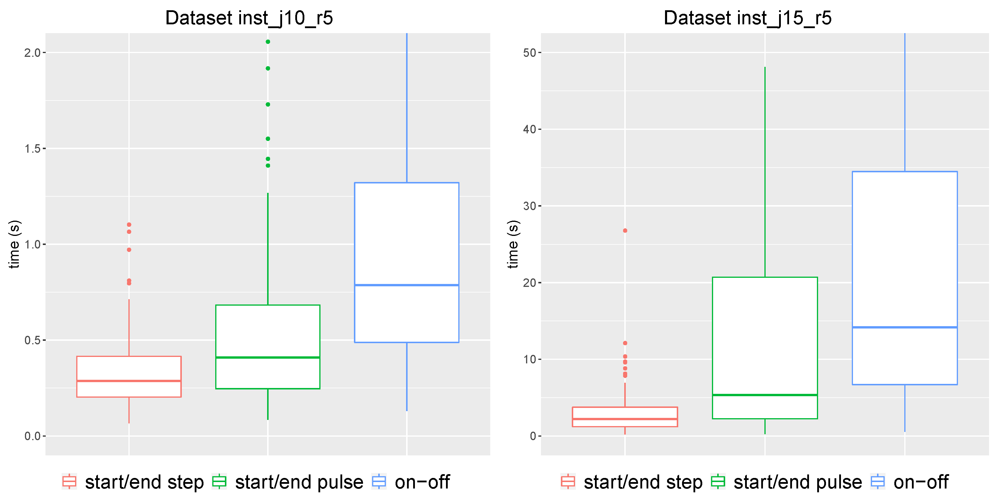
Figure 2 presents solution times obtained for these two datasets with three different model versions.

We can conclude that the best performance in terms of solution time is obtained for generalized model with step formulation of scheduling constraints. This type of constraints has been also used in models of Baydoun et al. [10] and Bianco et al. [16]. In next sections, we use the generalized model with step start and end variables (presented in Section 2.2.3) to compare it with an aggregated fraction approach.

3. Aggregated Fraction Model and Generalized Model: Comparison

3.1. Structural Model Compliance

In order to obtain the model used by Baydoun et al. [10] and Bianco et al. [16], it is sufficient to replace all variables $c_{jrt}$ by expression $W_{jr}{f}_{jt}$. Here $f_{jt}\in [0,1]$ is an aggregated fraction continuous decision variable used to make decision about all resources involved in job implementation. There is another way to make our formulation equivalent to these models: We can strengthen the model with a constraint:

$$\frac{c_{j{r}_{1}t}}{W_{j{r}_1}}=\frac{c_{j{r}_{2}t}}{W_{j{r}_2}}\forall j\in J,\forall r_1,r_2\in R,\forall t\in T.$$

(27)

In this case, all values of $f_{jt}$ have to be identical for every pair of resource.

Further, we compare our generalized model with the aggregated fraction model. For this comparison, the aggregated fraction model is obtained by using $f_{jt}\in [0,1]$ instead of $c_{jrt}$ and with the transformation $c_{jrt}=W_{jr}{f}_{jt}$ in all corresponding constraints.

3.2. Time to Obtain the Proofed Optimal Solution

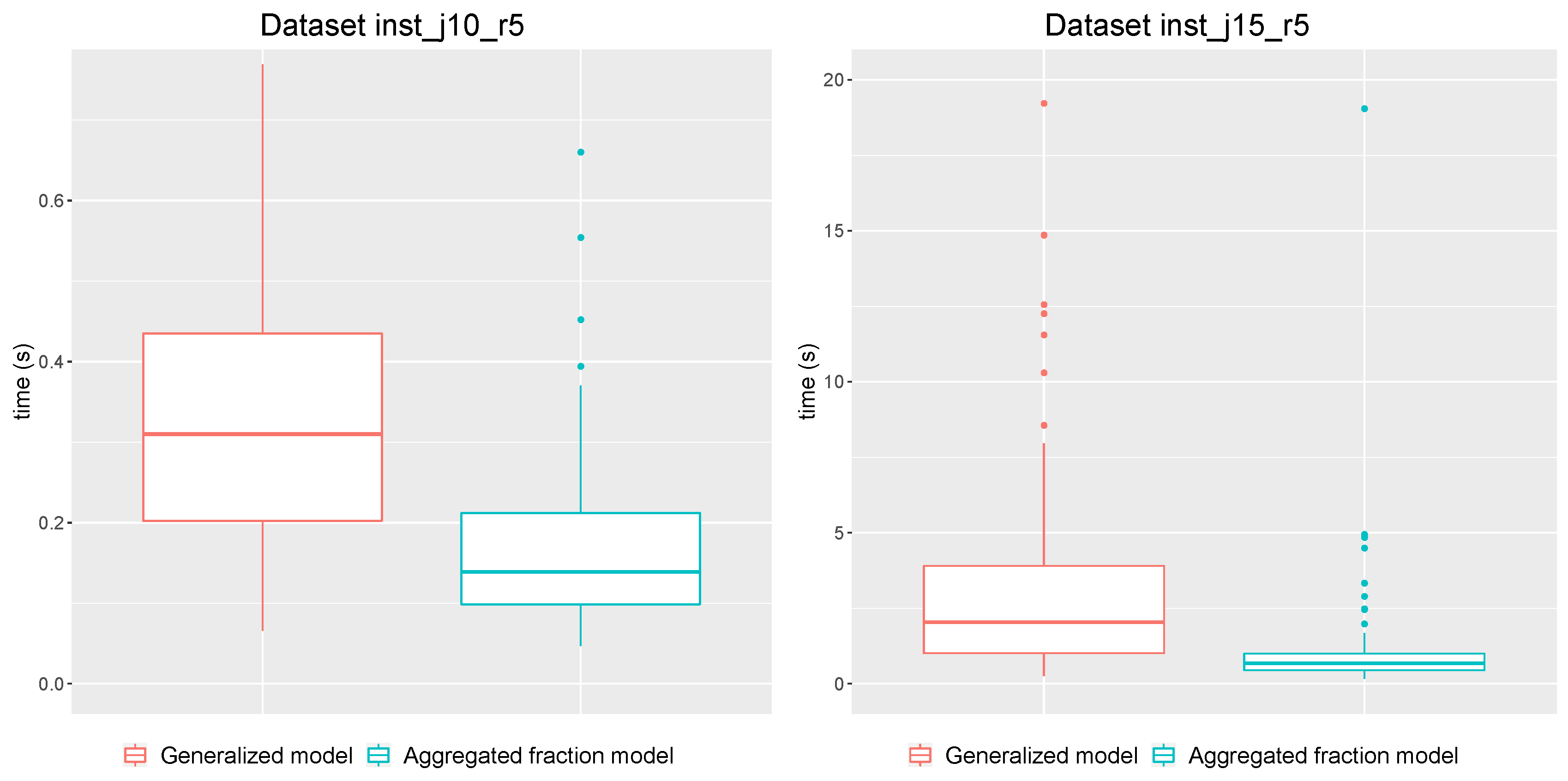
Firstly, we run both models and compare the time spent to construct the optimal solution. The results presented in Figure 3 confirm that the larger generalized model is slower.

3.3. Solution Quality

However, the generalized model provides more flexible solutions that allow to get much better solutions in terms of the objective function value. Denote an optimal solution objective function value for instance I of the generalized model and aggregated fraction model, respectively, as $V_g(I)$ and $V_{af}(I)$, and $X(I)$ as the ratio of these values,

$$X(I)=V_g(I)/V_{af}(I).$$

In

Table 4. $X(I)$ values for instances of datasets $inst\_j10\_r5$ and $inst\_j15\_r5$.

Data Set	Min	Q1	Median	Mean	Q3	Max
$inst\_j10\_r5$	0.17	0.41	0.49	0.48	0.55	0.71
$inst\_j15\_r5$	0.25	0.42	0.51	0.50	0.56	0.72

there is summary data of $X(I)$ for two datasets of instances. On average, in both cases the solution provided by generalized model has two times less objective function value.

3.4. Reasons to Use the Generalized Model

Suppose there is a resource leveling problem without any special requirements for synchronized resource occupation for one job, i.e., both models are acceptable. Is it reasonable to use generalized model if it has worse performance? To answer this question, we make the following experiment: For each instance from dataset we run the generalized model with time limit which equals the execution time of aggregated fraction model. In other words, we compare the aggregated fraction model optimal solution with suboptimal solution of generalized model obtained in same time. Results are presented in

Table 5. $X(I)$ value summary for instances of datasets $inst\_j10\_r5$ and $inst\_j15\_r5$, with time limit equal to the optimal solution time for the aggregated fraction model.

Data Set	Min	Q1	Median	Mean	Q3	Max
$inst\_j10\_r5$	0.19	0.45	0.51	0.53	0.59	0.87
$inst\_j15\_r5$	0.25	0.46	0.55	0.55	0.61	0.9

.

We can conclude that for this dataset the ratio of aggregated fraction model optimal solution objective value to generalized model suboptimal solution objective function obtained remains about two times more as without time limits.

The value of $X(I)$ depends on the instance parameters. For example, if the availability of resources is higher in periods, then the objective function value decreases for both models. In this case, we obtain lower values of $X(I)$. We can demonstrate this on new datasets $inst\_j10\_r5\_2$ and $inst\_j15\_r5\_2$ with distribution $L_{rt}\in [0,140]$ instead of $L_{rt}\in [0,70]$, see

Table 6. $X(I)$ values for instances of datasets $inst\_j10\_r5\_2$ and $inst\_j15\_r5\_2$, in two cases: (a) without time limit and (b) with time limit equal to the optimal solution time for the aggregated fraction model.

Time limit	Data set	Min	Q1	Median	Mean	Q3	Max
(a) Not fixed	$inst\_j10\_r5\_2$	0.1	0.3	0.36	0.36	0.42	0.63
	$inst\_j15\_r5\_2$	0.04	0.26	0.32	0.32	0.39	0.52
(b) Aggregated fraction model	$inst\_j10\_r5\_2$	0.1	0.33	0.4	0.41	0.47	0.97
optimal solution construction time	$inst\_j15\_r5\_2$	0.09	0.27	0.37	0.36	0.43	0.59

.

We also make new experiments. In addition to datasets presented above, we generate larger instances and vary the number of resource types: We generate two datasets with 5 and 10 resource types and 30 jobs. In

Table 7. Instance dataset parameters.

Data Set	$\left|\mathit{T}\right|$	d	$\left|\mathit{J}\right|$	$\left|\mathit{R}\right|$	$\left|\mathit{P}\right|$	${\mathit{L}}_{\mathit{rt}}$	${\mathit{W}}_{\mathit{jr}}$	${\mathit{p}}_{\mathit{min},\mathit{jr}}$	${\mathit{p}}_{\mathit{max},\mathit{jr}}$	${\mathit{e}}_{\mathit{r}}$
$inst\_j30\_r5$	35	1	30	5	30	$[0.0,70.0]$	$[30.0,50.0]$	$[1.0,5.0]$	$[6.0,10.0]$	$[1.0,4.0]$
$inst\_j30\_r10$	35	1	35	10	30	$[0.0,70.0]$	$[30.0,50.0]$	$[1.0,5.0]$	$[6.0,10.0]$	$[1.0,4.0]$

we present the ranges used to generate each instance parameter. Each dataset contains 30 instances.

We note that there are several RLP benchmarks already introduced in the literature. Bianco et al. [16] used two RLP benchmarks. The first benchmark was described by Kolish et al. [21] and contained datasets with 10 and 20 jobs. The second benchmark contained datasets with 10, 20, and 30 jobs. It was presented by Schwindt [22]. These datasets were prepared for the formulation with fixed job duration and intensity. For the variable duration case Bianco et al. enriched the data with the following assumption: Initial duration was considered as the maximal value, while the minimal duration was obtained by multiplying it by 0.75. Project deadline was calculated as the longest path from 0 to $n+1$ job in the precedence graph. In some instances each job requires only one resource type. In both benchmarks the instances included 1, 3 or 5 resources.

In our research, we generate instances with the same size, but various parameters such as minimal and maximal duration of jobs and resource allocation limits. It is also important to demonstrate the difference in solution quality for the case when there are many resource types required to implement each job. For datasets $inst\_j30\_r5$ and $inst\_j30\_r10$ we set a 5 min time limit. In

Table 8. $X(I)$ value summary for instances of datasets $inst\_j30\_r5$ and $inst\_j30\_r5$, with a 5 min time limit.

Data Set	Min	Q1	Median	Mean	Q3	Max
$inst\_j30\_r5$	0.33	0.45	0.48	0.49	0.53	0.62
$inst\_j30\_r10$	0.42	0.49	0.51	0.51	0.54	0.58

we present the results for these datasets. We note that we compare suboptimal solutions, obtained in a given time limit.

We point out that in the same time the generalized model provides better solutions in all cases. Worst-case ratio of generalized model solution objective to aggregated model solution value is around 0.6. It is reached by the flexible solution structure, even with worse performance evaluated by reached relative gap. We illustrate the gap values in

Table 9. Relative gap value summary for instances of datasets $inst\_j30\_r5$ and $inst\_j30\_r5$, with 5 min time limit.

Data Set	Model	Min	Q1	Median	Mean	Q3	Max
$inst\_j30\_r5$	Aggregated fraction	0.004	0.011	0.016	0.018	0.023	0.053
	Generalized	0.05	0.11	0.16	0.16	0.19	0.3
$inst\_j30\_r10$	Aggregated fraction	0.007	0.01	0.012	0.014	0.019	0.032
	Generalized	0.07	0.12	0.14	0.16	0.18	0.38

to make conclusions about the real optimal objective function value. The aggregated fraction model has a low relative gap in all cases. No significant progress can be achieved by the aggregated fraction model with higher time limits, so it cannot outperform generalized model in solution quality.

Computational experiments confirm that we can achieve better solutions within the same solution time limit with the same solver if we apply the generalized formulation approach.

4. Discrete Resource Case

In the Objective Function (24), continuous overloading variables are used in order to calculate the cost of extra resources. It is compliant with such continuous resources as electricity or heat. However, in practice such resources as machines or human operators can be only available in discrete units. For this case, two possible models can be used.

• Firstly, decision variable $o_{rt}$ can be defined as integer with the minimal unit of each resource $q_r$. New variables $o_{rt}^{*}$ set the number of extra units used and they replace $o_{rt}$ in Objective Function (24) and Constraint (23):

  $$Minimize{\displaystyle \sum _{r\in R}}{\displaystyle \sum _{t\in T}}{e}_r{q}_r{o}_{rt}^{*};$$

  (28)

  $$q_r{o}_{rt}^{*}\ge {\displaystyle \sum _{j\in J}}{c}_{jrt}-L_{rt},\forall t\in T,\forall r\in R.$$

  (29)
  We define this model as $DO$ (discrete objective). This case can be used not only for discrete resources, but it also suits the usual practice when additional resources could be demanded in some packages, for example, the batteries.
• Secondly, it is also possible to define other decision variables related to resource allocation as integers. This corresponds to the case when we have discrete resources and we allocate a discrete amount of workload to all periods. We define this model as $DO\&R$ (discrete objective and resources).

A computational experiment has been run to compare the behavior of continuous and discrete versions of the model. Seven models with different types and parameters of overload variables were considered: The original model with continuous overload variables, three versions of the discrete model with different resource unit size $q_r=q$, $\forall r\in R$, equal to 1, 3, and 5, defined as $DO$, and the same values of q for the discrete resource allocation case defined as $DO\&R$.

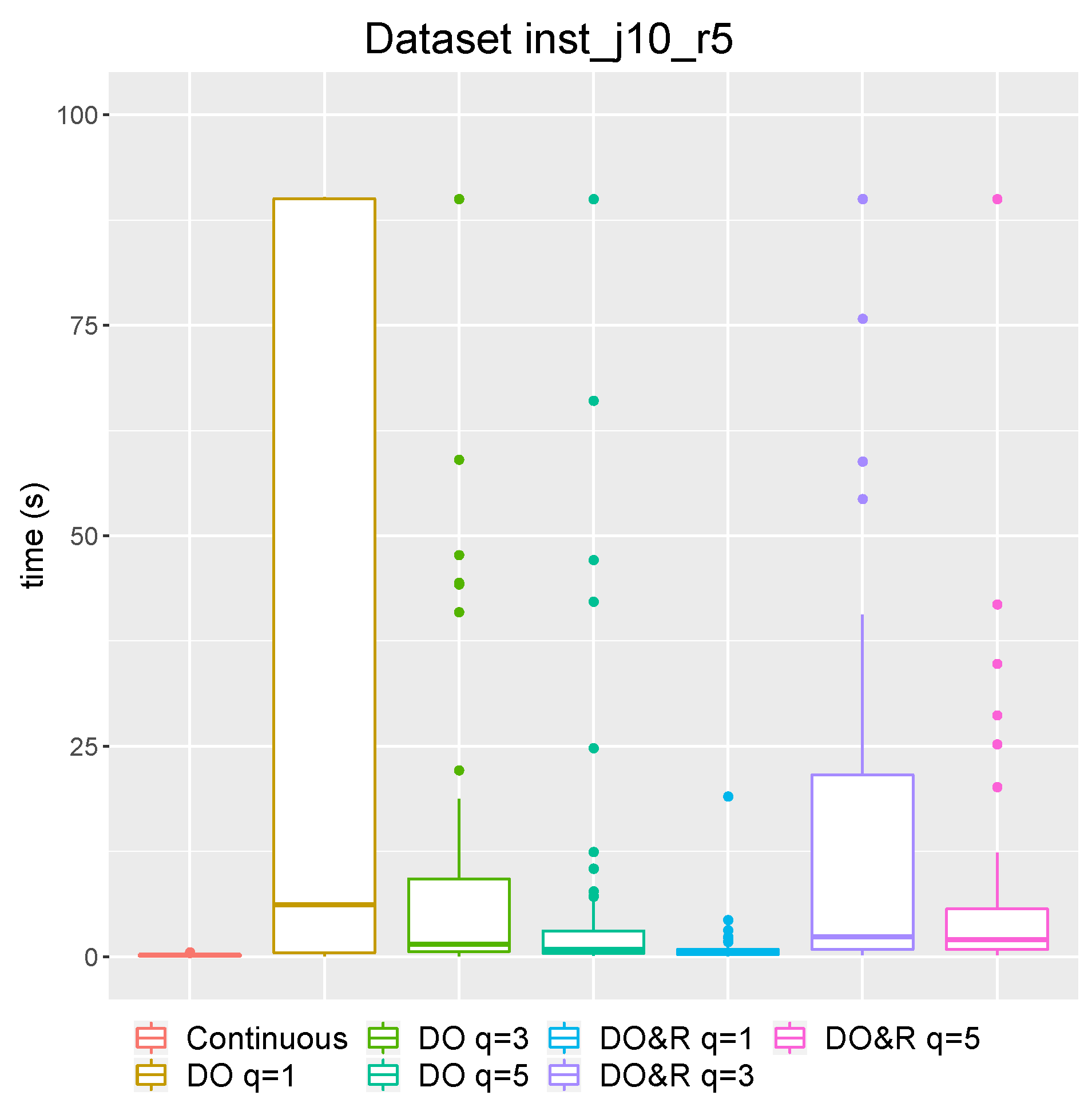
Figure 4 presents the computational results for dataset $inst\_j10\_r5$ with a 90 s time limit for all models. Each column is a boxplot that aggregates the data about the solution time, defining the median, lower and upper values, and quartiles. In addition,

Table 10. Mean values for different models.

Model Overload Type	Objective	Time, s	Gap	$\mathit{\delta }$
Continuous	471.5	0.18	0	-
$DO$ q = 1	474.1	38.3	0.001	0.006
$DO$ q = 3	487.4	18.6	0.001	0.04
$DO$ q = 5	502.6	8	0.0005	0.02
$DR\&O$ q = 1	482.5	0.9	0	0.06
$DR\&O$ q = 3	469.9	20.3	0.001	0.07
$DR\&O$ q = 5	471.5	12	0.001	0.09

provides the mean values of the objective function, solution time, and gap which was not presented in Figure 4. Here we also compare optimal solution objective function value provided by discrete model and continuous generalized model ($V_C$), and calculate relative delta. For example, for instance I and model $DO$ it is

$${\delta }_{V_{DO}}(I)=\frac{V_{DO}(I)-V_C(I)}{V_C(I)}$$

As could be expected, the computation time for the discrete model is higher than for the basic continuous model. For some part of the instances, no optimal solution was reached in 90 s for the discrete model, while all the instances were solved for the basic continuous model faster than in a second. However, the information about the gap provided by the solver shows that the main issue is in the proof of optimality: All instances had a very small gap value when the time limit was reached. It is also interesting that the second model type $DO\&R$ with the discrete allocation of resources provides optimal solutions much faster than the first type $DO$. Consequently, it is possible to use these discrete models with some reasonable small gap tolerance.

5. Conclusions

In this paper, we propose a new mathematical formulation for a resource leveling problem with a variable duration of jobs. We consider the extra resource usage cost as the objective function which has to be minimized. Extra resources are required because of a lack of available resources during a fixed planning horizon with a deadline. The main idea behind this new formulation is to provide a more flexible allocation of different resources to jobs, which allows obtaining solutions with better objective function values. Moreover, we consider different models for scheduling decision variables and constraints.

This new formulation approach is compared to other RLP formulations with overload which were found in the literature. We defined them as aggregated fraction models to underline the main difference. The numerical experiments show that, even if the generalized formulation uses more variables and constraints, it provides much better solutions. In this paper the primary goal was to present and evaluate an improvement in solution quality. We also had a secondary goal to demonstrate that our generalized model can compete with the aggregated fraction model with the same solver computational resource and time limit. We compared the proofed optimal solution of the aggregated fraction formulation with a suboptimal solution of a generalized formulation obtained at the same time. We can state that with the same solver and time limit, the generalized formulation also provides better solution quality. However, we did not test any acceleration methods for this RLP model.

There are two directions for further research. Firstly, it would be valuable to provide a theoretical estimation of the difference in the value of the objective function for the generalized and fraction-aggregated models. This would allow determining some subsets of instances with a maximum difference between solution quality. Secondly, with good perspectives in solution quality, it is reasonable to focus on model improvements and adapt existing RLP solution algorithms for the new model. This will require more tests with instances and the application of some resource leveling problem benchmark datasets for model performance comparison. Some particular real case-based problems may also inspire further steps. For example, scheduling of workforce with additional constraints such as variable experience depending on previous actions [23].

In order to improve the solution procedure, the development of a Benders decomposition algorithm is planned for future research. Besides, approximation schemes can be quite efficient as we can estimate the objective function value difference for the discrete and the continuous resource models, which provides the estimated accuracy if the scheme is based on the continuous model.

References

1. Blazewicz, J.; Lenstra, J.; Kan, A. Scheduling subject to resource constraints: Classification and complexity. Discret. Appl. Math. 1983, 5, 11–24. [Google Scholar] [CrossRef] [Green Version]
2. Neumann, K.; Schwindt, C.; Zimmermann, J. Resource-Constrained Project Scheduling—Minimization of General Objective Functions. In Project Scheduling with Time Windows and Scarce Resources: Temporal and Resource-Constrained Project Scheduling with Regular and Nonregular Objective Functions; Springer: Berlin/Heidelberg, Germany, 2002; pp. 175–299. [Google Scholar] [CrossRef]
3. Neubert, G.; Savino, M.M. Flow shop operator scheduling through constraint satisfaction and constraint optimisation techniques. Int. J. Prod. Qual. Manag. 2009, 4, 549–568. [Google Scholar] [CrossRef]
4. Rieck, J.; Zimmermann, J. Exact Methods for Resource Leveling Problems. In Handbook on Project Management and Scheduling; Schwindt, C., Zimmermann, J., Eds.; Springer International Publishing: Cham, Switzerland, 2015; Volume 1, pp. 361–387. [Google Scholar] [CrossRef]
5. Christodoulou, S.E.; Michaelidou-Kamenou, A.; Ellinas, G. Heuristic Methods for Resource Leveling Problems. In Handbook on Project Management and Scheduling; Schwindt, C., Zimmermann, J., Eds.; Springer International Publishing: Cham, Switzerland, 2015; Volume 1, pp. 389–407. [Google Scholar] [CrossRef]
6. Tadepalli, T.C.M. Genetic algorithm based optimization for resource leveling problem with precedence constrained scheduling. Int. J. Constr. Manag. 2019. [Google Scholar] [CrossRef]
7. Piryonesi, S.M.; Nasseri, M.; Ramezani, A. Resource leveling in construction projects with activity splitting and resource constraints: A simulated annealing optimization. Can. J. Civ. Eng. 2019, 46, 81–86. [Google Scholar] [CrossRef]
8. Li, H.; Wang, M.; Dong, X. Resource Leveling in Projects with Stochastic Minimum Time Lags. J. Constr. Eng. Manag. 2019, 145, 04019015. [Google Scholar] [CrossRef]
9. Cherkaoui, K.; Baptiste, P.; Pellerin, R.; Haït, A.; Perrier, N. Proactive tactical planning approach for large scale engineering and construction projects. J. Mod. Proj. Manag. 2017, 5, 96–105. [Google Scholar] [CrossRef]
10. Baydoun, G.; Haït, A.; Pellerin, R.; Cément, B.; Bouvignies, G. A rough-cut capacity planning model with overlapping. OR Spectr. 2016, 38, 335–364. [Google Scholar] [CrossRef] [Green Version]
11. Artigues, C.; Lopez, P.; Haït, A. The energy scheduling problem: Industrial case-study and constraint propagation techniques. Int. J. Prod. Econ. 2013, 143, 13–23. [Google Scholar] [CrossRef] [Green Version]
12. Capelle, M.; Huguet, M.J.; Jozefowiez, N.; Olive, X. Ground stations networks for Free-Space Optical communications: Maximizing the data transfer. Electron. Notes Discret. Math. 2018, 64, 255–264. [Google Scholar] [CrossRef] [Green Version]
13. Hans, E. Resource Loading by Branch-and-Price Techniques. Ph.D. Thesis, Twente University Press (TUP), Enschede, The Netherlands, 2001. [Google Scholar]
14. Kis, T. A branch-and-cut algorithm for scheduling of projects with variable-intensity activities. Math. Program. 2005, 103, 515–539. [Google Scholar] [CrossRef]
15. Bianco, L.; Caramia, M. Minimizing the completion time of a project under resource constraints and feeding precedence relations: A Lagrangian relaxation based lower bound. 4OR 2011, 9, 371–389. [Google Scholar] [CrossRef]
16. Bianco, L.; Caramia, M.; Giordani, S. Resource levelling in project scheduling with generalized precedence relationships and variable execution intensities. OR Spectr. 2016, 38, 405–425. [Google Scholar] [CrossRef]
17. Pritsker, A.A.B.; Watters, L.J.; Wolfe, P.M. Multiproject Scheduling with Limited Resources: A Zero-One Programming Approach. Manag. Sci. 1969, 16, 93–108. [Google Scholar] [CrossRef] [Green Version]
18. Kis, T.; Drótos, M. Hard Planning and Scheduling Problems in the Digital Factory. In Math for the Digital Factory; Ghezzi, L., Hömberg, D., Landry, C., Eds.; Springer International Publishing: Cham, Switzerland, 2017; pp. 3–19. [Google Scholar] [CrossRef] [Green Version]
19. Naber, A. Resource-constrained project scheduling with flexible resource profiles in continuous time. Comput. Oper. Res. 2017, 84, 33–45. [Google Scholar] [CrossRef]
20. Artigues, C.; Koné, O.; Lopez, P.; Mongeau, M. Mixed-Integer Linear Programming Formulations. In Handbook on Project Management and Scheduling; Schwindt, C., Zimmermann, J., Eds.; Springer International Publishing: Cham, Switzerland, 2015; Volume 1, pp. 17–41. [Google Scholar] [CrossRef]
21. Kolisch, R.; Schwindt, C.; Sprecher, A. Benchmark Instances for Project Scheduling Problems. In Project Scheduling: Recent Models, Algorithms and Applications; Węglarz, J., Ed.; Springer: Boston, MA, USA, 1999; pp. 197–212. [Google Scholar] [CrossRef]
22. Schwindt, C. Verfahren zur Lösung des ressourcenbeschränkten Projektdauerminimierungsproblems mit planungsabhängigen Zeitfenstern; Berichte aus der Betriebswirtschaft, Shaker: Aachen, Germany, 1998. [Google Scholar]
23. Karam, A.; Attia, E.A.; Duquenne, P. A MILP model for an integrated project scheduling and multi-skilled workforce allocation with flexible working hours. IFAC-PapersOnLine 2017, 50, 13964–13969. [Google Scholar] [CrossRef]
Figure 1. Three different ways to utilize binary scheduling variables.
Algorithms 13 00006 g001
Figure 2. Different model formulation time boxplots for instances of datasets i n s t _ j 10 _ r 5 and i n s t _ j 15 _ r 5 .
Algorithms 13 00006 g002
Figure 3. Time boxplots for datasets i n s t _ j 10 _ r 5 and i n s t _ j 15 _ r 5 .
Algorithms 13 00006 g003
Figure 4. Time boxplot for different cases of discrete objective and allocation for dataset i n s t _ j 10 _ r 5 .
Algorithms 13 00006 g004