Semi-Supervised Manifold Alignment Using Parallel Deep Autoencoders

Abstract

The aim of manifold learning is to extract low-dimensional manifolds from high-dimensional data. Manifold alignment is a variant of manifold learning that uses two or more datasets that are assumed to represent different high-dimensional representations of the same underlying manifold. Manifold alignment can be successful in detecting latent manifolds in cases where one version of the data alone is not sufficient to extract and establish a stable low-dimensional representation. The present study proposes a parallel deep autoencoder neural network architecture for manifold alignment and conducts a series of experiments using a protein-folding benchmark dataset and a suite of new datasets generated by simulating double-pendulum dynamics with underlying manifolds of dimensions 2, 3 and 4. The dimensionality and topological complexity of these latent manifolds are above those occurring in most previous studies. Our experimental results demonstrate that the parallel deep autoencoder performs in most cases better than the tested traditional methods of semi-supervised manifold alignment. We also show that the parallel deep autoencoder can process datasets of different input domains by aligning the manifolds extracted from kinematics parameters with those obtained from corresponding image data.

1. Introduction

Circles and lines are one-dimensional manifolds. Two-dimensional manifolds include surfaces such as spheres, tori and pretzels. Higher-dimensional manifolds include curved spaces that locally look like a Euclidean space. The mathematical definition of a topological n-dimensional manifold, or n-manifold, M, requires that M is a second countable Hausdorff space, and each each point in M has a neighbourhood that is homeomorphic to an open subset of the Euclidean space ${\mathbb{R}}^n$ [1,2,3].

Manifold learning refers to techniques of non-linear dimensionality reduction that can extract latent low-dimensional manifolds from high-dimensional data [4,5,6,7]. For example, we can consider the frames of a video where each frame can be regarded as a pixel vector of a few thousand dimensions. If the video shows a rotating object or if the camera rotates in a circle, then manifold learning techniques such as isomap [5] can extract a circle from the video frame sequence, which shows that the essential information contained in the high-dimensional data is that of a circular rotation, which can be visualised as a 1-manifold homeomorphic to $S^1$ in two dimensions [8]. If the object in the image sequence is not only rotated, but also translated, we obtain a manifold homeomorphic to $S^1\times I$, that is a cylinder [9]. A torus homeomorphic to $S^1\times S^1$ was obtained by [10] from an image set of robot heads that turn left and right in one circle or nod up and down in another circle.

Two major issues that can occur in the context of manifold learning are that there are not enough data or that the data are too noisy. Both issues can prevent the success of manifold learning, that is the extraction of an intact latent low-dimensional manifold from high-dimensional input data without it collapsing [4,11,12].

In this project, we focus on a variation of manifold learning called manifold alignment [13,14] that can extract manifolds even under suboptimal conditions. If there are not enough samples in the dataset, then manifold alignment can combine the information from two or more datasets to provide sufficient data. The datasets can be different high-dimensional representations of the same underlying non-linear manifold. Manifold alignment can also be used for data matching and information transfer between these datasets. There are several examples of application studies, for example, in face processing [14,15,16,17,18,19,20], graph matching [21,22], bioinformatics [23], and in image clustering and classification [24,25,26].

With respect to the issue of noise, autoencoder neural networks are a possible solution. It is known that neural networks are not only relatively robust to noise, but that the addition of noise to the data can even improve performance [27]. Basic autoencoders were already employed for dimensionality reduction in the 1980s, but had limitations to learn non-linear data patterns [28]. Hinton and Salakhutdinov [29] proposed deep autoencoders to reduce the dimensionality of images and to embed image sequences in a manifold. Several later studies demonstrated the usefulness of deep autoencoders for dimensionality reduction and manifold learning in various applications [30,31,32]. The ability of autoencoder neural networks to deal with noisy data was further established in several recent studies that developed deep autoencoders to denoise data, for example [33,34].

The present study combines the concept of deep neural networks with their robustness to noise and the concept of manifold alignment with its ability to utilise the information from two or more datasets to achieve successful manifold learning and proposes a Parallel Deep Autoencoder (PDAE) for manifold alignment. The approach can be regarded as semi-supervised because it is a combination of unsupervised learning for dimensionality reduction and supervised learning for aligning the manifolds using correspondence information in two input datasets.

The goal of our experimental study is to evaluate PDAE in comparison to several other relevant traditional manifold alignment methods. Specifically, we aim to demonstrate how these methods and PDAE perform on the task to extract manifolds up to dimension four with a non-trivial topology from high-dimensional data. As this is a challenging task, we start with ideal data conditions for semi-supervised manifold alignment and generate datasets that are sufficiently large and have clearly-defined correspondences. We also investigate how the task is affected by noise in the data. The sensitivity to noise and the high computational demands in time and memory are among the limiting abilities of traditional manifold alignment methods that made the extraction of non-trivial 3- and 4-manifolds very uncommon in previous studies.

We can further demonstrate that an asymmetric version of PDAE can be applied to cases where the two input datasets are of different modalities, for example a feature vector-based representation and an image-based representation. The ability to process data of two different modalities is another advantage of PDAE concept over traditional manifold alignment approaches.

Related application studies are emerging using biological data or standard datasets such as MNIST [35], MS-COCO, or Flickr data [36]. Wang et al. [37] proposed a parallel autoencoder framework for detection/identification of damage in multi-storey structures. Their parallel autoencoders reduced dimensionality and extracted features from frequency data and mode shape data. The results showed better accuracy in damage identification than a sparse auto-encoder-based framework. These studies showed that for real-world cases, where datasets can differ in representation and dimensionality, an asymmetric PDAE can be useful. However, in all these emerging application studies, the topology of the manifolds underlying the data was either trivial or was not determined.

2. Semi-Supervised Manifold Alignment

Ham et al. [14] characterised manifold alignment using the correspondence information of two input datasets that have subsets of corresponding point pairs as semi-supervised manifold alignment. These subsets of corresponding points are employed to establish the alignment of the two latent low-dimensional manifolds. Ham et al. [14] referred to points with correspondence information as “labelled” points. Among the semi-supervised manifold alignment methods, two approaches can be distinguished [38]:

• Approach I: Dimensionality reduction is followed by alignment [23].
• Approach II: A joint manifold is created to represent the union of the given manifolds, and then, the joint manifold is mapped to a lower-dimensional space [39].

For experimental comparison with the new PDAE, we employed the following three methods. Each is an example of one of the above two general approaches and can be applied at the feature level (feat) and at the instance level (inst) [39]:

• Method 1 (MAPA), Manifold Alignment using Procrustes Analysis [23]: This method is a version of Approach I and in its second step applies Procrustes analysis to rescale and rotate manifold $S_Y$ to align it with manifold $S_X$. If Locality Preserving Projections (LPP) [40] are used in the dimensionality reduction step, it results in feature-level manifold alignment, and we refer to the method as MAPA-feat in the following sections. If Laplacian eigenmaps [41] are used in the dimensionality reduction step to obtain instance-level alignment, we refer to the method as MAPA-inst.
• Method 2 (MALG), Manifold Alignment preserving Local Geometry [39]: This method is a version of Approach II. First, a joint manifold Z is calculated using the graph Laplacians of the given manifolds. If, in the next step, eigenvalue decomposition of Z provides instance-level alignment, we refer to it as MALG-inst. If generalised eigenvalue decomposition of Z is used for feature-level alignment, we refer to the method as MALG-feat.
• Method 3 (MAGG), Manifold Alignment preserving Global Geometry [39]: This method is a version of Approach II. A joint manifold Z is generated using the global distances of corresponding pairs in $X\cup Y$. Eigenvalue decomposition of Z provides dimensionality reduction to obtain the aligned low-dimensional manifolds in the case of instance-level alignment (MAGG-inst). Generalised eigenvalue decomposition is used instead in the case of feature-level alignment (MAGG-feat).

In summary, this classification comprises six semi-supervised manifold alignment methods: MAPA-feat, MAPA-inst, MALG-feat, MALG-inst, MAGG-inst, and MAGG-feat. These will be used in the following for comparisons with the proposed PDAE.

3. Parallel Deep Autoencoder

Let $A:{\mathbb{R}}^m⟶{\mathbb{R}}^p$ and $B:{\mathbb{R}}^p⟶{\mathbb{R}}^m$ be mappings representing the encoder and decoder parts, respectively, of an autoencoder, that maps an input vector $X\in {\mathbb{R}}^m$ to an output $\widehat{X}=B\circ A(X)$ of equal dimension where $A(X)$ at the code layer is p-dimensional with $p<m$. In a deep autoencoder, both mappings A and B comprise several layers [42].

The autoencoders of the present study use $p=3$, so that the code layer activations provide a compressed representation of the input that can be visualised as a 3D point cloud, which can approximate a manifold, for example a 2D surface in ${\mathbb{R}}^3$.

In our neural network-based approach to manifold alignment, two deep autoencoders are run in parallel (Figure 1). The two encoders $A_X$ and $A_Y$ embed the two datasets X and Y in 3D coded space as $S_X=A_X(X)$ and $S_Y=A_Y(Y)$, respectively. Then, the decoders $B_X$ and $B_Y$ try to reconstruct the data to $\widehat{X}=B_X(A_X(X))$ and $\widehat{Y}=B_Y(A_Y(Y))$ in ${\mathbb{R}}^m$.

If dataset X has n instances or points $X_1,\cdots ,X_n$ and each instance comprises m features, then X is represented as a $(n\times m)$-matrix where the instances correspond to the rows. Training is conducted to minimise the reconstruction errors $E(X,\widehat{X})={(\frac{1}{n}{\sum }_{i=1}^n{\parallel X_i-\widehat{X_i}\parallel }^2)}^{\frac{1}{2}}$ and $E(Y,\widehat{Y})={(\frac{1}{n}{\sum }_{i=1}^n{\parallel Y_i-\widehat{Y_i}\parallel }^2)}^{\frac{1}{2}}$. These two error functions are combined to obtain the total reconstruction error:

$$E_{recon}=E(X,\widehat{X})+E(Y,\widehat{Y}).$$

(1)

A correspondence error between the two code layers is calculated to regulate the alignment of the compressed data. $X_c\subset X$ and $Y_c\subset Y$ are defined as the subsets of corresponding points, that is selected pairs of points from both datasets that are in a one-to-one relationship and refer to the same state of the system. In the simulation experiments, $X_c\subset X$ and $Y_c\subset Y$ comprised a uniform selection of $v\%$ of the data of X and Y, respectively. When reducing the dimensionality of X and Y, also $X_c$ and $Y_c$ are mapped into 3D space, resulting in $D_X=A_X(X_c)\subset S_X$ and $D_Y=A_Y(Y_c)\subset S_Y$. The error between corresponding points in $D_X$ and $D_Y$ is calculated as:

$$E_{corr}=\sqrt[]{\frac{100}{v·n}\sum _{x_iϵD_X,y_iϵD_Y}{\parallel x_i-y_i\parallel }^2}$$

(2)

and we refer to it as the correspondence error. The aim of minimising $E_{corr}$ is to align the manifolds underlying the data closely in coded space so that they can support each other in establishing the joint latent manifold that underlies both datasets. Finally, the total model error is defined as:

$$E=\lambda E_{recon}+\mu E_{corr}$$

(3)

Parameters $\lambda$ and $\mu$ can be tuned to put more emphasis on the dimensionality reduction aspects or the alignment aspect of the model. The parameter setting $\lambda =\mu =1$ was sufficient to demonstrate the desired abilities of PDAE for our study. These weight parameters may require careful re-adjustment on other more complex data. By minimising $E_{recon}$, the deep autoencoders try to learn the intrinsic manifolds in X and Y separately. The simultaneous minimisation of $E_{recon}$ and $E_{corr}$ reduces the distance of the code layer outputs where a joint three-dimensional representation of the datasets is generated, that is the parallel model trained by minimising the total error E extracts the intrinsic manifolds at the code layer and simultaneously aligns them.

Asymmetric PDAE

We also developed an asymmetric version of PDAE to perform manifold alignment in situations where the two datasets represent two different input modalities (Figure 2). Specifically, we considered the case where dataset X is a sample set of feature vectors and dataset Y comprises images. The framework is the same as in the symmetric case above with the difference being that one of the two autoencoders is replaced by a convolutional autoencoder (CAE), that is a fully-connected autoencoder (FAE) was used to reduce the dimensionality of X to $S_X$ and a CAE was used to reduce the dimensionality of the image dataset Y to $S_Y$. In our experiments, the code layer of both autoencoders had dimension three, and both datasets were assumed to be different high-dimensional representations of the same latent manifold. The input layer of the CAE had five kernels with a dimension equal to the pixel dimension of the input images in Y. In the encoder part, the CAE had multiple convolutional layers with maxpooling and dropout layers, and the decoder part mirrored this architecture. The errors $E_{recon}$, $E_{corr}$ and E were calculated similarly as in Equations (1)–(3). The gradient for training was applied to the total hyper-parameter set of PDAE.

4. Performance Evaluation

The main tool for performance evaluation in the present study is the qualitative visual assessment of the resulting manifold visualisations. This is supported by a quantitative evaluation, which takes into account that method-associated scaling effects can affect the distances between corresponding points. To counteract this effect, these distances were normalised by the maximum Euclidean distance of points on each of the manifolds as follows:

$$D_i=\frac{\parallel S_X(i)-S_Y(i)\parallel }{{max}_{\begin{array}{c}j=1,\cdots ,n\\ k=1,\cdots ,n\end{array}}(\parallel S_X(j)-S_X(k)\parallel ,\parallel S_Y(j)-S_Y(k)\parallel )}$$

(4)

where $S_X(i)$ and $S_Y(i)$ are corresponding points for $i=1,\cdots ,n$. Note that in the present study, all datasets are constructed so that each point in X has a corresponding point in Y. This allows calculating the matching error $\mathsf{\Delta }=({\sum }_{i=1}^n{D}_i)/n$ as the average of the normalised Euclidean distances $D_i,i=1,\cdots ,n$. Smaller distances between corresponding points usually indicate more close alignments. Hence, $\mathsf{\Delta }$ reflects the proximity of two aligned manifolds in low-dimensional space, which we considered as a measure of the quality of an alignment. In addition, we considered the standard deviation:

$$\sigma =\sqrt{(\sum _{i=1}^n{(D_i-\mathsf{\Delta })}^2)/n}$$

(5)

as a measure of the smoothness of an alignment. Note that when using more general datasets, other more general performance measures such as maximum mean discrepancy, KL divergence, or correlation matrices would be required as is common, for example, in the field of domain adaption [43].

5. Experiments and Results

In the experiments, the proposed PDAE approach and the six above discussed traditional manifold alignment methods were compared to extract and align pairs of 1-, 2-, 3-, and 4-dimensional manifolds. A well-known benchmark dataset that contains protein structure manifolds in three dimensions [44] was used in experiments that resulted in the extraction and alignment of one-dimensional manifolds. The other datasets were new and generated specifically for our study in simulation. They were the main datasets of our study and comprised high-dimensional motion data representing the dynamics of two double pendulums with different degrees of freedom. This data were used for a series of manifold alignment experiments that resulted in the extraction and alignment of manifolds homeomorphic to $S^1\times S^1$, $S^1\times S^2$, and $S^2\times S^2$, which were 2-, 3-, and 4-manifolds, respectively. For testing the asymmetric PDAE, one of the $S^1\times S^1$ datasets was replaced by a corresponding image sequence of the pendulum motion. The traditional manifold alignment methods were executed in MATLAB 2016, and the autoencoders were developed, trained, and executed using TensorFlow 1.3.1 with Python 3.5.

5.1. 1-Manifold Alignment

The dataset stemmed from the Protein Data Bank at Brookhaven National Laboratories [44]. It contains one-dimensional manifolds representing the structure of the glutaredoxin protein PDB-1G7O. The protein structure can be described in three-dimensional space as a chain of amino acids, that is the structures are 1-manifolds in three-dimensional space. The dataset comprises 21 models of the glutaredoxin protein and provides for each model 215 points in 3D. Models 1 and 21 were previously used for method evaluation by articles on manifold alignment using Procrustes analysis [23] and manifold alignment preserving local geometry [39]. We followed their example and used the same models to test our PDAE. To examine the robustness of the methods, the dataset generated from Model 21 was scaled by a factor of four because previous publications on manifold alignment did the same when testing the robustness of their methods [22,23,39,45,46]. Figure 3a shows the three-dimensional graphs of Models 1 and 21 where the $x,y$, and z coordinates of each model were the columns of the input data matrices X and Y, respectively.

Datasets X and Y were aligned by MAPA, MALG, MAGG, and PDAE. PDAE had nine fully-connected layers, where the architecture of the encoder network was 3-4-5-4-, the code layer had three neurons, and the decoder architecture was -4-5-4-3, that is it mirrored the encoder. The $tanh$ function was applied to the output of each layer as the activation function. The network was trained for 10,000 epochs using the Adam optimiser with a learning rate of $0.001$ and stopping condition $E\le 0.0008$.

The graphs of the resulting aligned manifolds shown in Figure 3b indicated that the outcome of MAPA-feat was not as robust as that of the other methods in Figure 3c–h. The manifolds aligned by the parallel autoencoders in Figure 3h were as well-aligned and as accurate as the MALG and MAGG methods from Approach 2 in Figure 3d–f.

We calculated $\mathsf{\Delta }$ and $\sigma$ of the aligned manifolds for each method. The results in

Table 1. The table shows $\mathsf{\Delta }$ of the alignment of Models 1 and 21 for all methods that were tested and visualised in Figure 3. The standard deviation $\sigma$ is provided in parenthesis. PDAE performed the best.

Methods		$\mathsf{\Delta }(\mathit{\sigma })$
MAPA	feat	0.094 (0.039)
	inst	0.030 (0.021)
MALG	feat	0.022 (0.016)
	inst	0.023 (0.021)
MAGG	feat	0.033 (0.024)
	inst	0.034 (0.030)
PDAE		0.017(0.010)

show that PDAE was the best performer. PDAEs were executed 10 times with 10 different sets of randomly-initialised weights. The standard deviation of $\mathsf{\Delta }$ for the basic autoencoder was $0.009$ and for the deep autoencoder was $0.003$. This showed that the selection of the initial weights did not have much impact on the autoencoder results.

5.2. Experiments on 2-, 3- and 4-Manifold Alignment

5.2.1. Double Pendulum Datasets

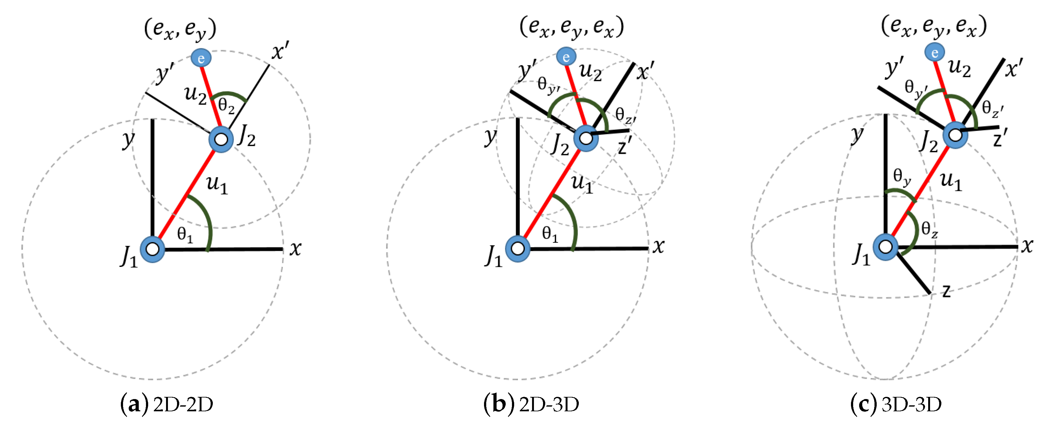
We generated high-dimensional datasets by simulating the motion of double pendulums where three different conditions were considered (Figure 4): 2D-2D, 2D-3D and 3D-3D. The two limbs of the double pendulum are denoted as $u_1$ and $u_2$, and the joints are denoted as $J_1$ and $J_2$. One end of $u_1$ is fixed at $R_1$, and the limb can rotate around this joint. The other end of $u_1$ is attached to $u_2$ at joint $R_2$. $u_2$ can rotate freely around joint $J_2$. The free end point e of the pendulum is referred to as the “end-effector” and has coordinates $\left(e_x,e_y\right)$ in the two-dimensional case and $\left(e_x,e_y,e_z\right)$ in the three-dimensional version using a right-handed coordinate system with the origin at joint $J_1$.

The data were generated in simulation for the 2D-2D, 2D-3D and 3D-3D cases as follows (Figure 4):

(i)

2D-2D motion: The pendulum has two Degrees-Of-Freedom (DOF), that is, both limbs $u_1$ and $u_2$ rotate in the two-dimensional (x-y)-plane, each of them describing a circle. In Figure 4a, ${\theta }_1$ and ${\theta }_2$ are the rotation angles of limbs $u_1$ and $u_2$ at joints $J_1$ and $J_2$, respectively. Accordingly, the manifold representing the dynamics of the 2D-2D case is the cross-product of two circles, $S^1\times S^1$, which is homeomorphic to the two-dimensional torus, that is a 2-manifold.

(ii)

2D-3D motion: The pendulum has three DOFs, where limb $u_2$ can rotate on a two-dimensional sphere $S^2$ in three-dimensional space, while $u_1$ is restricted to rotate on a circle $S^1$ in a two-dimensional plane. That is, the manifold representing the dynamics of the 2D-3D case is homeomorphic to $S^1\times S^2$, which is a 3-manifold. As the pendulum moves in 3D space, the end-effector has the 3D coordinates $\left(e_x,e_y,e_z\right)$. In Figure 4b, ${\theta }_{y^{\prime }}$ and ${\theta }_{z^{\prime }}$ are the angles of $u_2$ with axes $y^{\prime }$ and $z^{\prime }$, respectively, and describe the motion on the sphere $S^2$. ${\theta }_1$ is the angle between the x-axis and $u_1$ and describes the two-dimensional rotation of the sphere’s centre in the (x-y)-plane.

(iii)

3D-3D motion: In this case, the pendulum has four DOFs, where both limbs can rotate on two-dimensional spheres in 3D space. In Figure 4c, ${\theta }_y$ and ${\theta }_z$ are the angles of $u_1$ with the y and z axes, respectively, and ${\theta }_{y^{\prime }}$ and ${\theta }_{z^{\prime }}$ are the angles of $u_2$ with the $y^{\prime }$ and $z^{\prime }$ axes, respectively. Accordingly, we expected that the manifolds representing the dynamics of the 3D-3D case were homeomorphic to $S^2\times S^2$, which is a 4-manifold.

For each case, two datasets, X and Y, were generated that represented the motion of two similar double pendulums that differed only in different limb lengths and limb length ratios:

• Pendulum X: $(u_2/u_1)=0.75/1.25=0.60$
• Pendulum Y: $(u_2/u_1)=1.25/1.56=0.80$

that is, we restricted the experiments to the case $u_2<u_1$.

The feature vectors for each sample point (or instance) were calculated from the kinematics at the joints and the coordinates of the end-effector. The end-effector coordinates were calculated using forward kinematics. Then, feature vectors for the 2D-2D, 2D-3D, and 3D-3D cases were defined as:

• 2D-2D: $(e_x,e_y,cos{\theta }_1,cos{\theta }_2,sin{\theta }_1,sin{\theta }_2)$
• 2D-3D: $(e_x,e_y,e_z,cos{\theta }_1,cos{\theta }_{y^{\prime }},cos{\theta }_{z^{\prime }},sin{\theta }_1,sin{\theta }_{y^{\prime }},sin{\theta }_{z^{\prime }})$
• 3D-3D: $(e_x,e_y,e_z,cos{\theta }_y,cos{\theta }_z,cos{\theta }_{y^{\prime }},cos{\theta }_{z^{\prime }},sin{\theta }_z,sin{\theta }_y,sin{\theta }_{y^{\prime }},sin{\theta }_{z^{\prime }})$

The data points for the 2D double pendulums were generated using its equations of motion and then sampled at angular increments of ${10}^{\circ }$ in ${\theta }_1$ and ${\theta }_2$ at both joints. There were ${(360/10)}^2=1296$ instances and six features, resulting in a dataset of size $1296\times 6$ for each of the pendulums X and Y.

In the case of the 2D-3D motion, instances were sampled at angular increments of ${30}^{\circ }$ at three angles ${\theta }_1$, ${\theta }_{y^{\prime }}$ and ${\theta }_{z^{\prime }}$ of the corresponding joints. As a result, the number of instances was ${(360/30)}^3=1728$, and with the nine features, the size of the two datasets, X and Y, was $1728\times 9$.

In the 3D-3D case, instances were sampled at angular increments of ${30}^{\circ }$ in the rotational angles ${\theta }_y$, ${\theta }_z$, ${\theta }_{y^{\prime }}$ and ${\theta }_{z^{\prime }}$ at the corresponding joints. As a result, the number of instances was ${(360/30)}^4=$ 20,736, and with the 11 features, the size for each of the two datasets X and Y was 20,736 × 11.

In order to challenge the robustness of the different alignment methods and to simulate potential real-world scenarios, two different types of noise were added in separate experiments to the clean datasets X and Y. The first type of noise we refer to as “actuator noise”, and it was added to the joint angles to imitate the noise at actuator joints in a real-world system. The range of actuator noise was incremented from $0^{\circ }$ to $[-{10}^{\circ },{10}^{\circ }]$ in steps of $2^{\circ }$. The second type of noise was added to the end-effector coordinates, and we refer to it as “coordinate noise”. This noise could simulate, for example, the jittery motion of robot limbs. In the experiments, the coordinate noise range was increased from $0.0$ to $[-1.0,1.0]$ in steps of size $0.2$.

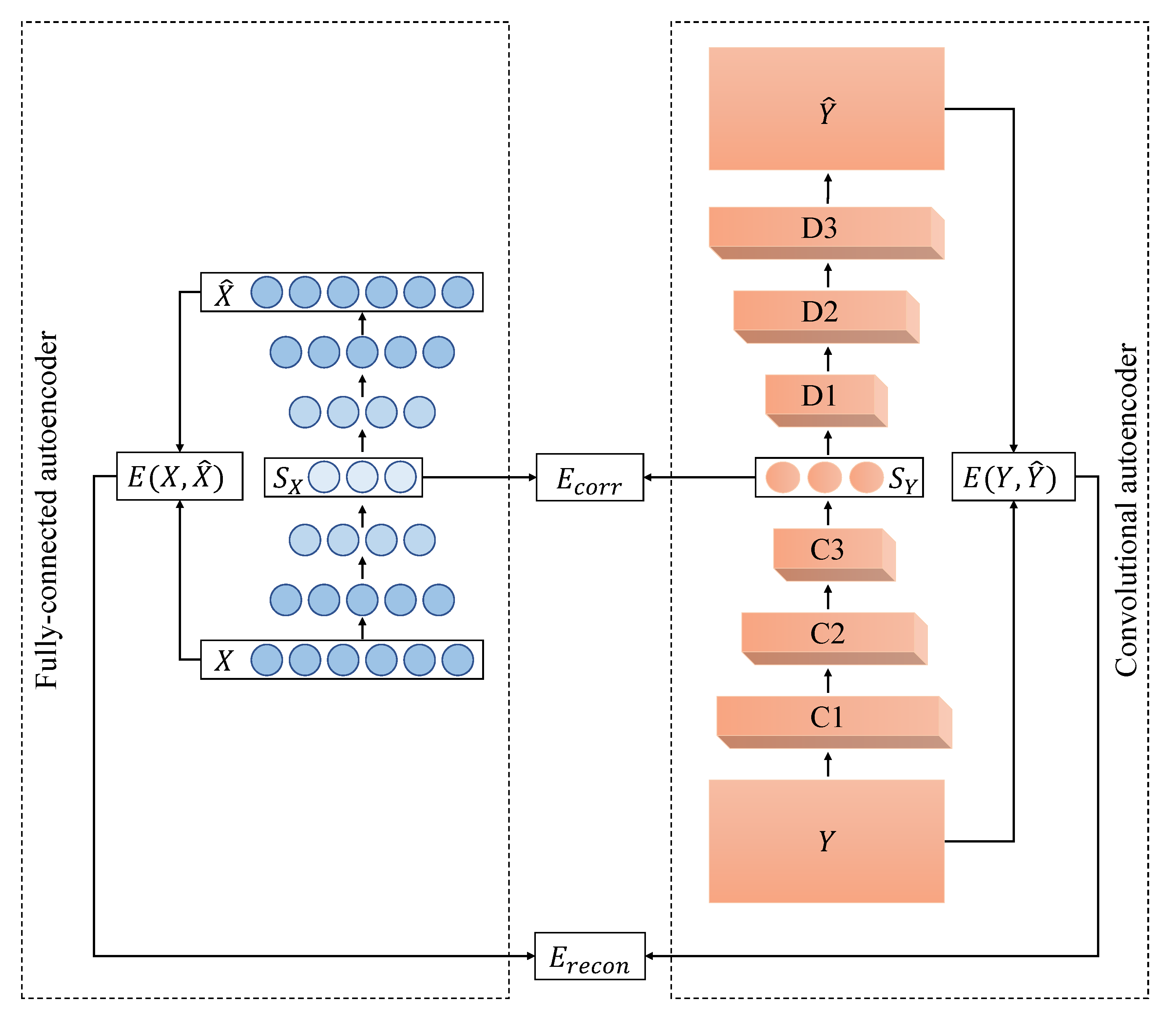
5.2.2. PDAE Architecture

The deep autoencoders that were used as part of PDAE had six neurons in the input layer for 2D-2D motion alignment where the data matrix had six features. Similarly, for the 2D-3D data, the input layer had nine neurons, and for the 3D-3D motion, the input layer had 11 neurons. Then, the number of neurons was reduced by one in each of the consecutive hidden layers until it reached three at the code layer of the deep autoencoders. The decoder had the same layer architecture as the encoder, but in reverse order. In summary, the architectures of the deep autoencoders were:

• 2D-2D: 6-5-4-3-4-5-6
• 2D-3D: 9-8-7-6-5-4-3-4-5-6-7-8-9
• 3D-3D: 11-10-9-8-7-6-5-4-3-4-5-6-7-8-9-10-11

The weights of the autoencoders were randomly initialised within $[-1,1]$ using a normal distribution. We plotted the network error for learning rates in the range $[0.0001,0.05]$ for 500 epochs to find the best performing learning rate using the Adam optimiser, which was $0.01$ for the 2D-2D case and $0.001$ for the 2D-3D and 3D-3D cases. Then, PDAEs were trained for 10,000 epochs with a stopping criterion of $E_{total}\le 0.001$ and $tanh$ as the activation function.

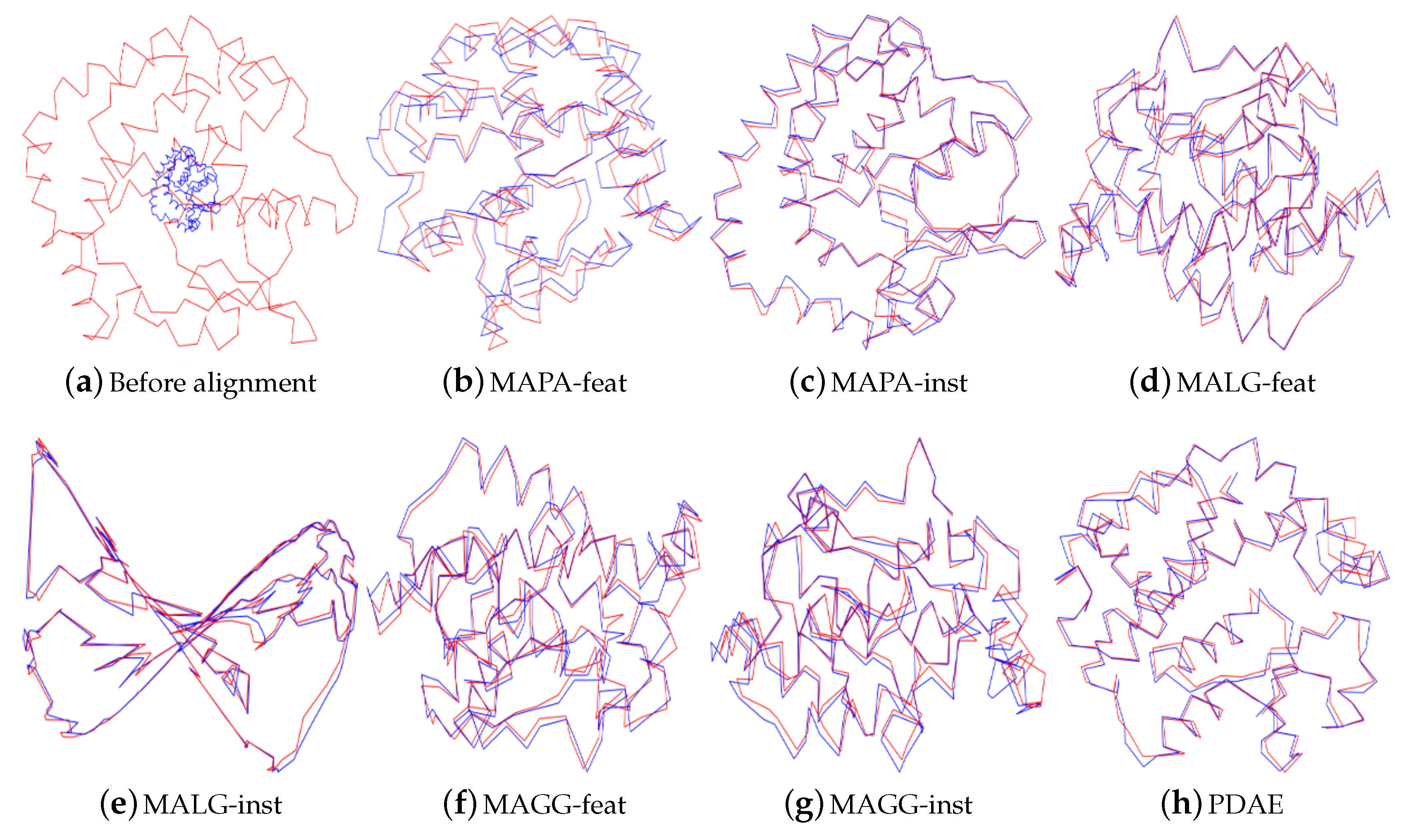
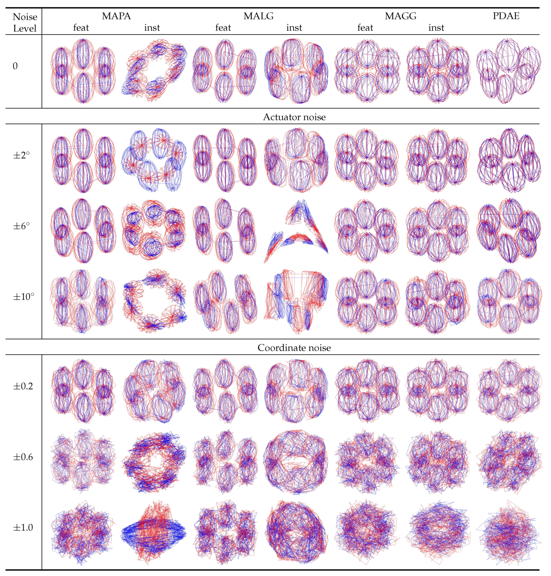
5.2.3. Results of 2-Manifold Alignment

In the case of the 2D-2D motion data, limb $u_l$ rotated around joint $J_1$ in a circle and limb $u_2$ rotated in another circle around joint $J_2$. In three-dimensional space, this motion can be represented as a torus $S^1\times S^1$, that is a 2-manifold. In the first row of Figure 5, we can see that for zero noise, the visualisations of the results for MAPA-inst, MALG and PDAE resulted in objects that resembled the expected torus-shaped surfaces, while the other methods produced cylinder-like deformations of torus-shaped surfaces. With increasing levels of noise (only three representative levels are displayed), the instance-level alignments were less stable than the feature-level alignments. The addition of noise led all traditional methods to fail by collapsing the resulting manifolds or misaligning the two sets. Visually, the best outcomes were achieved by PDAE where for all levels of noise, an object resembling a torus-like surface with minor deformations was obtained.

The alignment errors $\mathsf{\Delta }$ in

Table 2. 2D-2D manifold alignment: Shown are the alignment errors $\mathsf{\Delta }$ for the different alignment methods under different levels of noise. The standard deviation $\sigma$ as defined as a measure of smoothness of the alignment in (5) is provided in parenthesis. The best results are highlighted in bold.

Noise	MAPA		MALG		MAGG		PDAE
	feat	inst	feat	inst	feat	inst
0	0.186 (0.070)	0.112 (0.041)	0.003 (0.001)	0.013 (0.012)	0.054 (0.015)	0.089 (0.038)	0.007 (0.003)
Actuator noise
$\pm 2^{\circ }$	0.090 (0.030)	0.090 (0.037)	0.016 (0.009)	0.034 (0.026)	0.053 (0.017)	0.097 (0.043)	0.015(0.009)
$\pm 6^{\circ }$	0.377 (0.157)	0.485 (0.205)	0.047 (0.027)	0.101 (0.092)	0.072 (0.031)	0.098 (0.051)	0.011 (0.028)
$\pm {10}^{\circ }$	0.365 (0.154)	0.713 (0.304)	0.078 (0.043)	0.180 (0.135)	0.119 (0.055)	0.101 (0.056)	0.007(0.039)
Coordinate noise
$\pm 0.2$	0.105 (0.035)	0.150 (0.067)	0.039(0.018)	0.061 (0.042)	0.078 (0.029)	0.117 (0.052)	0.048 (0.022)
$\pm 0.6$	0.125 (0.056)	0.184 (0.093)	0.124 (0.056)	0.145 (0.096)	0.139 (0.060)	0.161 (0.076)	0.085(0.043)
$\pm 1.0$	0.203 (0.078)	0.271 (0.145)	0.135 (0.063)	0.218 (0.144)	0.204 (0.086)	0.190 (0.083)	0.128(0.048)

indicate that MALG-feat resulted in the closest alignment among the conventional methods. The $\mathsf{\Delta }$ of the autoencoder was lower than that of MALG-feat for higher levels of noise. Table 2 also shows that PDAE had the lowest standard deviation (in parentheses) at high levels of noise. This indicates that PDAE more smoothly aligned than the other methods. It should be noted that low values for $\mathsf{\Delta }$ or $\sigma$ can also occur when a torus manifold cannot correctly be established and uniformly collapses or projects into a simpler form as, for example, a cylinder in some cases of MALG-feat. We trained and tested PDAE with five different sets of initial random weights, and the standard deviation of the mean of the resulting alignment errors was about $0.0005$ at zero noise. This indicates that the autoencoder results do not depend in a notable way on the selection of the initial random weights.

5.2.4. Results of 3-Manifold Alignment

In the case of the 2D-3D motion data, limb $u_1$ rotated around joint $J_1$ in a circle and limb $u_2$ rotated on a two-dimensional sphere around joint $J_2$. In 3D space, this motion is represented by a manifold homeomorphic to $S^1\times S^2$ and can be visualised by a circle of spheres. For clearer visualisation of the quality of the alignments, we plotted only six of the aligned spheres equally distributed along the circle in Figure 6. The figures indicate visually (best if enlarged) that already for zero noise, the visualisations of the results of all methods had alignment issues except PDAE, which produced a near-perfect alignment. The alignment errors $\mathsf{\Delta }$ and $\sigma$ in

Table 3. 2D-3D manifold alignment: Alignment errors with standard deviations as explained in Table 2.

Noise	MAPA		MALG		MAGG		PDAE
	feat	inst	feat	inst	feat	inst
0	0.079 (0.032)	0.157 (0.073)	0.025 (0.012)	0.124 (0.055)	0.023 (0.012)	0.062 (0.025)	0.007 (0.004)
Actuator noise
$\pm 2^{\circ }$	0.065 (0.027)	0.427 (0.17)	0.025 (0.012)	0.092 (0.063)	0.026 (0.013)	0.037 (0.018)	0.012(0.006)
$\pm 4^{\circ }$	0.073 (0.031)	0.379 (0.153)	0.035 (0.017)	0.109 (0.06)	0.029 (0.016)	0.048 (0.025)	0.026(0.012)
$\pm 6^{\circ }$	0.065 (0.3)	0.115 (0.049)	0.039 (0.021)	0.273 (0.228)	0.048 (0.023)	0.074 (0.038)	0.051 (0.026)
$\pm 8^{\circ }$	0.150 (0.071)	0.082 (0.04)	0.052 (0.031)	0.207 (0.244)	0.047 (0.027)	0.086 (0.047)	0.062(0.026)
$\pm {10}^{\circ }$	0.120 (0.056)	0.169 (0.08)	0.089 (0.045)	0.361 (0.164)	0.078 (0.042)	0.117 (0.062)	0.049(0.023)
Coordinate noise
$\pm 0.2$	0.073 (0.031)	0.143 (0.075)	0.066 (0.025)	0.131 (0.066)	0.08 (0.031)	0.092 (0.044)	0.075 (0.033)
$\pm 0.4$	0.113 (0.047)	0.428 (0.169)	0.101 (0.041)	0.163 (0.095)	0.122 (0.05)	0.141 (0.071)	0.082 (0.035)
$\pm 0.6$	0.149 (0.061)	0.182 (0.095)	0.131 (0.053)	0.197 (0.121)	0.171 (0.069)	0.185 (0.09)	0.139 (0.059)
$\pm 0.8$	0.215 (0.088)	0.384 (0.139)	0.159 (0.065)	0.237 (0.139)	0.238 (0.098)	0.230 (0.113)	0.088 (0.038)
$\pm 1$	0.264 (0.104)	0.438 (0.148)	0.196 (0.079)	0.297 (0.167)	0.297 (0.122)	0.315 (0.154)	0.119 (0.05)

corroborate the visual assessment and show that PDAE was the best-performing method in the experiments using the 2D-3D data.

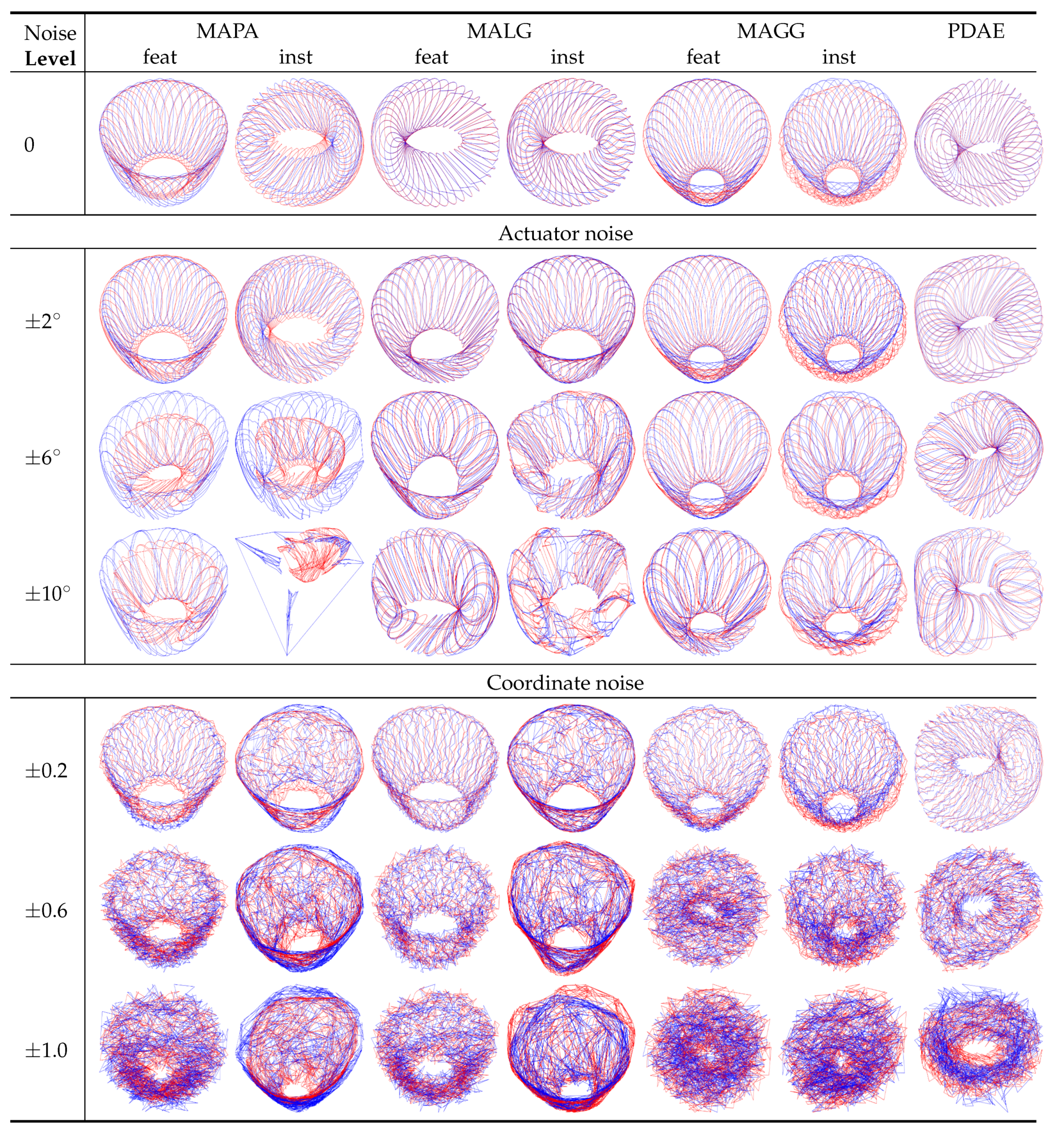
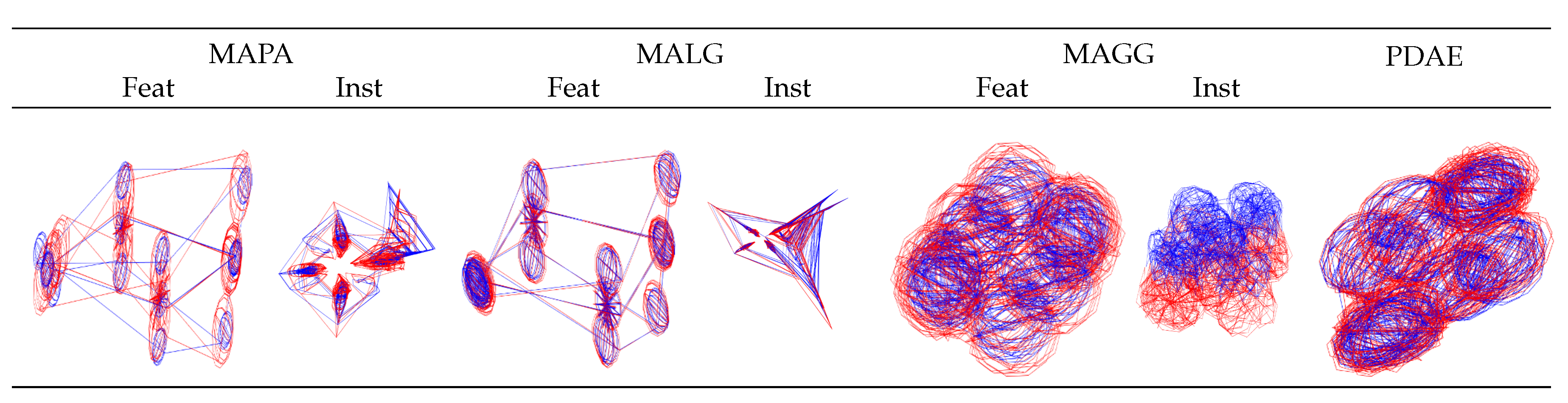
5.2.5. Results of 4-Manifold Alignment

The 11-dimensional data of the two 3D double pendulums were described in Section 5.2.1. Each of the two datasets X and Y was represented by a 20,736 × 11 data matrix. In the 3D pendulum motion, the rotation of limb $u_2$ described a sphere $S^2$, and the motion of the other limb $u_1$ described another sphere $S^2$, so that the 3D pendulum motion resembled $S^2\times S^2$, which is a 4-manifold. As this was too complex to visualise in full, we took snapshots of the motion around $J_1$ at ${90}^{\circ }$ steps and for the motion around $J_2$ at ${30}^{\circ }$ steps. This way, the rotation of $u_2$ resulted in six spherical shapes that were uniformly distributed on a bigger sphere, which represented the motion of $u_1$. The visualisations in Figure 7 show that the instance-level methods were not successful in aligning the high-dimensional nonlinear motion data. The manifolds of the instance-level alignments collapsed even without any noise. Only MAGG-feat and PDAE produced the expected visualisation, comprising six spheres that represented the snapshots we selected in the motion data on $S^2\times S^2$. The outcome of MAGG-feat was also supported by our case study [47].

For the remaining experiments, random noise was added to the data in several stages as described in Section 5.2.1. The noisy datasets were aligned using MAPA-feat, MALG-feat and PDAE. All manifolds collapsed after noise addition, and therefore, only visualisations for zero noise are included in Figure 7. $\mathsf{\Delta }$ and $\sigma$ were calculated as described in Section 4. The numerical results in

Table 4. 3D-3D manifold alignment: Shown is the alignment error $\mathsf{\Delta }$ with the standard deviation for each level of the noise. The lowest $\mathsf{\Delta }$ or closest alignment of each row is highlighted in bold.

Noise	MAPA	MALG	MAGG	PDAE
	feat	feat	feat
0	0.106 (0.060)	0.019(0.011)	0.045 (0.012)	0.037 (0.020)
Actuator noise
$\pm 2^{\circ }$	0.115 (0.067)	0.025(0.011)	0.048 (0.015)	0.029 (0.20)
$\pm 4^{\circ }$	0.124 (0.072)	0.042 (0.021)	0.058 (0.022)	0.039(0.019)
$\pm 6^{\circ }$	0.141 (0.077)	0.051 (0.025)	0.075 (0.032)	0.042(0.013)
$\pm 8^{\circ }$	0.233 (0.118)	0.058 (0.033)	0.082 (0.036)	0.050(0.037)
$\pm {10}^{\circ }$	0.359 (0.225)	0.066 (0.030)	0.090 (0.041)	0.054(0.016)
Coordinate noise
$\pm 0.2$	0.135 (0.078)	0.032 (0.015)	0.071 (0.012)	0.023(0.012)
$\pm 0.4$	0.151 (0.083)	0.048 (0.028)	0.113 (0.042)	0.024(0.013)
$\pm 0.6$	0.170 (0.094)	0.057 (0.033)	0.158 (0.058)	0.022(0.011)
$\pm 0.8$	0.213 (0.121)	0.072 (0.041)	0.194 (0.069)	0.070(0.033)
$\pm 1$	0.227 (0.122)	0.083 (0.047)	0.225 (0.079)	0.069(0.033)

together with the qualitative visual evaluations of Figure 7 showed that PDAE performed better than MAGG-feat and the other methods.

The experiments were executed on the university’s high performance computing grid with 60 GB RAM using two parallel k80 GPUs. The huge speed advantage of inference with the autoencoder was representative of all our data and all comparative simulations we conducted (Table 6). However, these speed results can only be indicative for precise benchmarking of a standalone high-performance machine or a specialised setup would be required.

5.3. Cross-Modality Manifold Alignment

The following pilot case study was included to demonstrate the cross-modality ability of the asymmetric PDAE concept. The 2D-2D kinematics dataset of double pendulum motion as described in Section 5.2.1 was used as dataset X and image frames of a simulated video of the same motion were used as dataset Y. Dataset X had 1296 instances, where each instance was a six-dimensional feature vector. Dataset Y had the same number of instances where each instance was an image with $128\times 128$ pixels. The datasets were generated and ordered so that each instance $X_i$ of X had a corresponding instance $Y_i$ in Y obtained from the same joint angles.

In the asymmetric PDAE, the structure of the fully-connected autoencoder was similar to the autoencoder used to align the 2-manifolds described in Section 5.2.2. The structure of the Convolutional Autoencoder (CAE) is given in

Table 5. Shown is the structure of the convolutional autoencoder part of the asymmetric PDAE, which was used to align our cross-modality pendulum data. The input layer is at the top.

Layer Type	Kernel	Channels	Size	Activation
Convolutional	5 × 5	3	128 × 128	lrelu
Max pool	2 × 2		56 × 56
Convolutional	5 × 5	10	56 × 56	lrelu
Max pool	2 × 2		28 × 28
Convolutional	5 × 5	20	28 × 28	lrelu
Max pool	2 × 2		14 × 14
Convolutional	5 × 5	30	14 × 14	lrelu
Max pool	2 × 2		7 × 7
Convolutional	3 × 3	40	7 × 7	lrelu
Max pool	2 × 2		4 × 4
Flatten			640
Fully-connected			200	tanh
Fully-connected			100	tanh
Fully-connected			3	tanh
Fully-connected			100	tanh
Fully-connected			200	tanh
Fully-connected			640	tanh
Reshape			4 × 4 × 40
Deconvolutional	3 × 3	40	4 × 4	lrelu
Upsampling	2 × 2		7 × 7
Convolutional	3 × 3	30	7 × 7	lrelu
Upsampling	2 × 2		14 × 14
Convolutional	5 × 5	20	14 × 14	lrelu
Upsampling	2 × 2		28 × 28
Convolutional	5 × 5	30	28 × 28	lrelu
Upsampling	2 × 2		56 × 56
Convolutional	5 × 5	40	56 × 56	lrelu
Upsampling	2 × 2		128 × 128
Convolutional	5 × 5	3	128 × 128	lrelu

. The asymmetric PDAE was trained for 10,000 epochs using the Adam optimiser with a learning rate of 0.0001.

Manifold alignment experiments using the asymmetric PDAE were conducted in four different ways, each using a differently-sized correspondence subset for the calculation of $E_{corr}$. The sizes of the correspondence subsets in the four experiments were $10\%$, $30\%$, $50\%$ and $100\%$ of the total number of instances. The results using the four different correspondence subsets are shown in Figure 8. The figures show that the more correspondence pairs were used, the better the alignment could be performed.

6. Discussion and Conclusions

While previous research had shown that deep autoencoders are capable of manifold learning, this study introduced a parallel deep autoencoder model for manifold alignment. The present study focused on semi-supervised approaches where parts of the data were labelled by correspondence information. Future studies may address the general case of data without correspondence information and a wider range of datasets.

In the new parallel model, two deep autoencoder networks were trained in parallel to minimise the sum of their reconstruction errors and a correspondence error. The minimisation of the reconstruction errors led the deep autoencoders to extract manifolds intrinsic to the datasets. The minimisation of the correspondence error aligned the extracted manifolds at the code layer. The activations at the 3D code layers allowed visualising the aligned manifolds or sections of them in three dimensions.

First, PDAE was evaluated on a well-known protein structure benchmark dataset, where it performed comparably to traditional manifold alignment methods.

Then, in the main part of our study, PDAE was tested on a suite of new 6-dimensional, 9-dimensional, and 11-dimensional datasets that we generated by simulating the non-linear dynamics of two double pendulums and adding various levels of noise. It should be noted that manifold learning and manifold alignment can be computationally very expensive (

Table 6. Shown are the execution times of the different manifold alignment methods when processing our data. The dataset sizes were $1296\times 6$, $1728\times 9$, and 20,736 × 11 for the 2-, 3- and 4-manifold data, respectively. The training times of the PDAE were recorded for 10,000 epochs and averaged over five runs starting from different initial weights. Standard deviations are in parenthesis. The other methods did not involve randomness, and their execution times remained the same in repeat experiments.

Methods	Detail	Execution Times
		2-Manifold Alignment	3-Manifold Alignment	4-Manifold Alignment
MAPA	feat	0.63 s	2.2 min	6.6 min
	inst	0.71 s	4.2 min	13.9 min
MALG	feat	0.32 s	1.6 min	5.3 min
	inst	0.44 s	3.7 min	11.7 min
MAGG	feat	3 s	9.5 min	11 h
	inst	8 s	12.3 min	13 h
PDAE	training	18 (3.88) min	22 (5.56) min	9.3 (5.22) h
	inference	0.33 (0.04) s	0.61 (0.08) s	1.6 (0.12) s

). Hence, the experiments of our comparative study were restricted to two pendulums with similar arm-length proportions. With this data, the expected resulting manifolds were of sufficient complexity to challenge the methods, but could still be visualised either in full as two-dimensional tori in three-dimensional space (Figure 5) or using snapshots or sections of the resulting 3-manifolds (Figure 6) or 4-manifolds (Figure 7).

Interestingly, the visualisation of the aligned manifold obtained from the two three-dimensional pendulum motion datasets on the right in Figure 7 together with the numerical evaluation in Table 4 indicated that, even in this unexampled case of representing a latent 4-manifold, PDAE produced the expected outcome and performed better than all other tested methods. In fact, all methods failed except PDAE and MAGG-feat. The quantitative performance evaluation in Table 4 shows that the alignment using PDAE was closer and more stable than that of MAGG. Moreover, due to the involvement of high-dimensional matrix multiplication, MAGG required a significantly higher execution time than the other methods (Table 6).

Table 6 summarises the execution times for all methods used in our study when applied to the clean and complete versions of our simulated datasets. While training of the PDAE took a long time, the inference, that is the execution time using the trained neural model, was significantly faster than running the other methods. It is important to note that if new data points are included in the dataset, the trained model of PDAE can still be executed while the other methods require recalculation.

MAGG calculates the distances between the two datasets at the input, which have to be of a common fixed dimension. In contrast, PDAE can be designed to take two datasets of different dimensions as inputs. For example, in the experiments in Section 5.3, PDAE demonstrated successful alignment of data of two different modalities and of different dimensions.

In summary, the results of the reported manifold alignment experiments showed that PDAE performed competitively and in most cases better than the traditional methods MAPA, MALG and MAGG. When synthetic random noise was added to the data at the actuator and the end-effector, the alignment using the new PDAE was often still possible and more stable than that of all other methods that were used for comparison.

The addition of noise is a critical contribution in this type of study using manifolds of dimension larger than one, as in traditional manifold learning, there is a substantial risk that the topology of the resulting manifolds cannot be established or collapses if there are not enough data or if there is any disturbance or noise in the data [11,12].

It is due to these issues that traditional manifold alignment struggled to become popular in applications and that the present study had to confine itself to simulated data to achieve expressive comparative results. Nonetheless, the torus surface $S^1\times S^1$, the 3-manifold $S^1\times S^2$ and the 4-manifold $S^2\times S^2$ were topologically more complex manifolds than the manifolds underlying the data of most previous studies on manifold alignment. The experiments of our study showed that the concept of PDAE allowed manifold alignment to result in manifolds of non-trivial topology.

We hope that the new PDAE model with its fast inference times, its robustness to noise and its ability to process datasets of different dimensions and to extract manifolds of 2, 3, 4 or more dimensions will open new opportunities for applications of semi-supervised manifold alignment.

References

1. Lee, J.M. Introduction to Topological Manifolds; Springer: New York, NY, USA, 2000. [Google Scholar]
2. Hirsch, M. Differential Topology; Springer: New York, NY, USA, 2000. [Google Scholar]
3. Spivac, M. A Comprehensive Introduction to Differential Geometry, 2nd ed.; Publish or Perish, Inc.: Houston, TX, USA, 1979. [Google Scholar]
4. Lee, J.A.; Verleysen, M. Nonlinear Dimensionality Reduction; Springer Science & Business Media: New York, NY, USA, 2007. [Google Scholar]
5. Tenenbaum, J.B.; de Silva, V.; Langford, J.C. A global geometric framework for nonlinear dimensionality reduction. Science 2000, 290, 2319–2323. [Google Scholar] [CrossRef] [PubMed]
6. Van Der Maaten, L.; Postma, E.; Van den Herik, J. Dimensionality Reduction: A Comparative Review; Technical Report TiCC TR 2009-005; Tilburg Center for Cognition and Communication (TiCC): Tilburg, The Netherlands, 2009. [Google Scholar]
7. Ma, Y.; Fu, Y. (Eds.) Manifold Learning. Theory and Applications; CRC Press, Inc.: Boca Raton, FL, USA, 2011. [Google Scholar]
8. Chalup, S.K.; Clement, R.; Tucker, C.; Ostwald, M.J. Modelling Architectural Visual Experience Using Non-linear Dimensionality Reduction. In Proceedings of the Australian Conference on Artificial Life (ACAL 2007), Gold Coast, Australia, 4–6 December 2007; Lecture Notes in Computer Science. Randall, M., Abbass, H., Wiles, J., Eds.; Springer: Berlin/Heidelberg, Germany, 2007; Volume 4828, pp. 84–95. [Google Scholar]
9. Chalup, S.K.; Clement, R.; Marshall, J.; Tucker, C.; Ostwald, M.J. Representations of Streetscape Perceptions Through Manifold Learning in the Space of Hough Arrays. In Proceedings of the 2007 IEEE Symposium on Artificial Life (CI-ALife 2007), Honolulu, HI, USA, 1–5 April 2007; IEEE: Piscataway, NJ, USA, 2007; pp. 362–369. [Google Scholar] [Green Version]
10. Wong, A.S.W.; Chalup, S.K.; Bhatia, S.; Jalalian, A.; Kulk, J.; Nicklin, S.; Ostwald, M.J. Visual Gaze Analysis of Robotic Pedestrians Moving in Urban Space. Archit. Sci. Rev. 2012, 55, 213–223. [Google Scholar] [CrossRef]
11. Paul, R.; Chalup, S.K. A Study on Validating Non-Linear Dimensionality Reduction Using Persistent Homology. Pattern Recognit. Lett. 2017, 100, 160–166. [Google Scholar] [CrossRef]
12. Aziz, F.; Chalup, S. Testing the Robustness of Manifold Learning on Examples of Thinned-Out Data. In Proceedings of the 2019 International Joint Conference on Neural Networks (IJCNN 2019), Budapest, Hungary, 14–19 July 2019; IEEE: Piscataway, NJ, USA, 2019. [Google Scholar]
13. Ham, J.H.; Lee, D.D.; Saul, L.K. Learning high dimensional correspondences from low dimensional manifolds. In Proceedings of the 20th International Conference on Machine Learning (ICML 2003) Workshop: The Continuum from Labeled to Unlabeled Data in Machine Learning and Data Mining, Washington, DC, USA, 21–24 August 2003. [Google Scholar]
14. Ham, J.; Lee, D.; Saul, L. Semisupervised alignment of manifolds. In Proceedings of the Annual Conference on Uncertainty in Artificial Intelligence, The Savannah Hotel, Barbados, 6–8 January 2005. [Google Scholar]
15. Chang, Y.; Hu, C.; Feris, R.; Turk, M. Manifold Based Analysis of Facial Expression. Image Vis. Comput. 2006, 24, 605–614. [Google Scholar] [CrossRef]
16. Cui, Z.; Shan, S.; Zhang, H.; Lao, S.; Chen, X. Image sets alignment for video-based face recognition. In Proceedings of the 2012 IEEE Conference on Computer Vision and Pattern Recognition (CVPR), Providence, RI, USA, 16–21 June 2012; pp. 2626–2633. [Google Scholar] [CrossRef]
17. Pei, Y.; Huang, F.; Shi, F.; Zha, H. Unsupervised image matching based on manifold alignment. IEEE Trans. Pattern Anal. Mach. Intell. 2012, 34, 1658–1664. [Google Scholar] [CrossRef] [PubMed]
18. Wang, X.; Yang, R. Learning 3D shape from a single facial image via non-linear manifold embedding and alignment. In Proceedings of the 2010 IEEE Conference on Computer Vision and Pattern Recognition (CVPR), San Francisco, CA, USA, 13–18 June 2010; pp. 414–421. [Google Scholar] [CrossRef]
19. Xiong, L.; Wang, F.; Zhang, C. Semi-definite manifold alignment. In Machine Learning: ECML 2007; Lecture Notes in Computer Science, Book Section 79; Kok, J., Koronacki, J., Mantaras, R., Matwin, S., Mladenič, D., Skowron, A., Eds.; Springer: Berlin/Heidelberg, Germany, 2007; Volume 4701, pp. 773–781. [Google Scholar]
20. Zhai, D.; Li, B.; Chang, H.; Shan, S.; Chen, X.; Gao, W. Manifold alignment via corresponding projections. In Proceedings of the British Machine Vision Conference, Aberystwyth, UK, 31 August–3 September 2010; BMVA Press: Surrey, UK, 2010; pp. 1–11. [Google Scholar] [CrossRef]
21. Escolano, F.; Hancock, E.; Lozano, M. Graph matching through entropic manifold alignment. In Proceedings of the 2011 IEEE Conference on Computer Vision and Pattern Recognition (CVPR), Colorado Springs, CO, USA, 20–25 June 2011; pp. 2417–2424. [Google Scholar] [CrossRef]
22. Abeo, T.A.; Shen, X.J.; Ganaa, E.D.; Zhu, Q.; Bao, B.K.; Zha, Z.J. Manifold alignment via global and local structures preserving PCA framework. IEEE Access 2019, 7, 38123–38134. [Google Scholar] [CrossRef]
23. Wang, C.; Mahadevan, S. Manifold alignment using procrustes analysis. In Proceedings of the 25th International Conference on Machine Learning, ICML ’08, Helsinki, Finland, 5–9 July 2008; ACM: New York, NY, USA, 2008; pp. 1120–1127. [Google Scholar] [CrossRef]
24. Guerrero, R.; Ledig, C.; Rueckert, D. Manifold alignment and transfer learning for classification of Alzheimer’s disease. In Machine Learning in Medical Imaging; Wu, G., Zhang, D., Zhou, L., Eds.; Springer: Cham, Switzerland, 2014; pp. 77–84. [Google Scholar]
25. Yang, H.L.; Crawford, M.M. Manifold alignment for multitemporal hyperspectral image classification. In Proceedings of the 2011 IEEE International Geoscience and Remote Sensing Symposium (IGARSS), Vancouver, BC, Canada, 24–29 July 2011; pp. 4332–4335. [Google Scholar] [CrossRef]
26. Li, X.; Lv, J.; Zhang, Y. Manifold Alignment Based on Sparse Local Structures of More Corresponding Pairs. In Proceedings of the Twenty-Third International Joint Conference on Artificial Intelligence (IJCAI’13), Beijing, China, 3–9 August 2013; pp. 2862–2868. [Google Scholar]
27. Bishop, C.M. Training with Noise is Equivalent to Tikhonov Regularization. Neural Comput. 1995, 7, 108–116. [Google Scholar] [CrossRef]
28. Bourlard, H.; Kamp, Y. Auto-association by multilayer perceptrons and singular value decomposition. Biol. Cybern. 1988, 59, 291–294. [Google Scholar] [CrossRef] [PubMed]
29. Hinton, G.E.; Salakhutdinov, R.R. Reducing the Dimensionality of Data with Neural Networks. Science 2006, 313, 504–507. [Google Scholar] [CrossRef] [PubMed] [Green Version]
30. Sakurada, M.; Yairi, T. Anomaly Detection Using Autoencoders with Nonlinear Dimensionality Reduction. In Proceedings of the MLSDA 2014 2nd Workshop on Machine Learning for Sensory Data Analysis, MLSDA’14, Gold Coast, Australia, 2 December 2014; ACM: New York, NY, USA, 2014; pp. 4–11. [Google Scholar] [CrossRef]
31. Wang, Y.; Yao, H.; Zhao, S. Auto-encoder Based Dimensionality Reduction. Neurocomputing 2016, 184, 232–242. [Google Scholar] [CrossRef]
32. Finn, C.; Tan, X.Y.; Duan, Y.; Darrell, T.; Levine, S.; Abbeel, P. Deep spatial autoencoders for visuomotor learning. In Proceedings of the 2016 IEEE International Conference on Robotics and Automation (ICRA), Stockholm, Sweden, 16–21 May 2016; pp. 512–519. [Google Scholar] [CrossRef]
33. Vincent, P.; Larochelle, H.; Lajoie, I.; Bengio, Y.; Manzagol, P.A. Stacked denoising autoencoders: Learning useful representations in a deep network with a local denoising criterion. J. Mach. Learn. Res. 2010, 11, 3371–3408. [Google Scholar]
34. Majumdar, A. Blind denoising autoencoder. IEEE Trans. Neural Netw. Learn. Syst. 2018, 30, 1–6. [Google Scholar] [CrossRef] [PubMed]
35. Amodio, M.; Krishnaswamy, S. MAGAN: Aligning Biological Manifolds. In Proceedings of the 35th International Conference on Machine Learning, ICML, Stockholm, Sweden, 10–15 July 2018; pp. 215–223. [Google Scholar]
36. Mukherjee, T.; Yamada, M.; Hospedales, T.M. Deep matching autoencoders. arXiv 2017, arXiv:1711.06047. [Google Scholar]
37. Wang, R.; Li, L.; Li, J. A novel parallel auto-encoder framework for multi-scale data in civil structural health monitoring. Algorithms 2018, 11, 112. [Google Scholar] [CrossRef]
38. Wang, C.; Mahadevan, S. Manifold Alignment Without Correspondence. In Proceedings of the 21st International Joint Conference on Artificial Intelligence, IJCAI’09, Pasadena, CA, USA, 11–17 July 2009; Morgan Kaufmann Publishers Inc.: San Francisco, CA, USA, 2009; Volume 2, pp. 1273–1278. [Google Scholar]
39. Wang, C.; Mahadevan, S. A general framework for manifold alignment. In Proceedings of the AAAI Fall Symposium: Manifold Learning and Its Applications, Arlington, VA, USA, 5–7 November 2009; AAAI Press: Menlo Park, CA, USA, 2009; pp. 79–86. [Google Scholar]
40. He, X.; Niyogi, P. Locality preserving projections. In Advances in Neural Information Processing Systems (NIPS 2003); Thrun, S., Saul, L.K., Schölkopf, B., Eds.; MIT Press: Cambridge, MA, USA, 2004; Volume 16, pp. 153–160. [Google Scholar]
41. Belkin, M.; Niyogi, P. Laplacian eigenmaps for dimensionality reduction and data representation. Neural Comput. 2003, 15, 1373–1396. [Google Scholar] [CrossRef]
42. Baldi, P. Autoencoders, unsupervised learning, and deep architectures. In Proceedings of the ICML Workshop on Unsupervised and Transfer Learning; Guyon, I., Dror, G., Lemaire, V., Taylor, G., Silver, D., Eds.; PMLR: Bellevue, WA, USA, 2012; Volume 27, pp. 37–49. [Google Scholar]
43. Wang, M.; Deng, W. Deep Visual Domain Adaptation: A Survey. arXiv 2018, arXiv:1802.03601. [Google Scholar] [CrossRef]
44. Berman, H.M.; Battistuz, T.; Bhat, T.N.; Bluhm, W.F.; Bourne, P.E.; Burkhardt, K.; Feng, Z.; Gilliland, G.L.; Iype, L.; Jain, S.; et al. The protein data bank. Acta Crystallogr. Sect. D 2002, 58, 899–907. [Google Scholar] [CrossRef] [PubMed]
45. Wang, C. A Geometric Framework for Transfer Learning Using Manifold Alignment. Ph.D. Thesis, Department of Computer Science, University of Massachusetts Amherst, Amherst, MA, USA, 2010. [Google Scholar]
46. Wang, J.; Zhang, X.; Li, X.; Du, J. Semi-Supervised Manifold Alignment With Few Correspondences. Neurocomputing 2017, 230, 322–331. [Google Scholar] [CrossRef]
47. Aziz, F.; Wong, A.S.W.; Welsh, J.S.; Chalup, S.K. Aligning manifolds of double pendulum dynamics under the influence of noise. In Proceedings of the 25th International Conference on Neural Information Processing (ICONIP 2018), Siem Reap, Cambodia, 13–16 December 2018; Lecture Notes in Computer Science (LNCS). Springer: Cham, Switzerland, 2018. [Google Scholar]
Figure 1. PDAE: The two high-dimensional datasets X and Y include correspondence subsets X C and Y C , resp., and are compressed to low-dimensional manifolds S X and S Y , where D X and D Y are the low-dimensional representations of X C and Y C , respectively. The minimisation of E c o r r applies regularisation pressure to D X and D Y to align the low-dimensional manifolds S X and S Y .
Algorithms 12 00186 g001
Figure 2. Architecture of asymmetric PDAE: The left autoencoder is a fully-connected autoencoder, which takes feature vectors from X as input. The right autoencoder is a CAE, which takes images from Y as input. Both autoencoders have a fully-connected layer with three neurons as their code layer.
Algorithms 12 00186 g002
Figure 3. Protein structure manifold alignment. 3D structure of the glutaredoxin protein PDB-1G7O: The blue graph shows Model 1, and the red graph shows Model 21 scaled by a factor of four. (a) shows the manifolds before alignment. The other subfigures show the resulting alignments using (b) MAPA-feature (feat), (c) MAPA-instance (inst), (d) MALG-feat, (e) MALG-inst, (f) MAGG-feat, (g) MAGG-inst and (h) PDAE.
Algorithms 12 00186 g003
Figure 4. (a) shows the 2D-2D version of the double pendulum where both limbs are rotating in a two-dimensional plane. x and y are the local coordinate axes of limb u 1 . x and y are the local axes of limb u 2 . ( e x , e y ) are the end-effector coordinates. (b) shows the 2D-3D version of the double pendulum where limb u 1 is in a two-dimensional plane and limb u 2 is rotating on a sphere in three-dimensional space. x and y are the local coordinate axes of limb u 1 . x , y and z are the local coordinate axes of limb u 2 , and ( e x , e y , e z ) are the end-effector coordinates. (c) shows the 3D-3D version of the double pendulum where both limbs are rotating on spheres in three-dimensional space. x, y and z are the local axes of limb u 1 . x , y and z are the local axes of limb u 2 , and ( e x , e y , e z ) are the end-effector coordinates.
Algorithms 12 00186 g004
Figure 5. Manifold alignments of 2D motion data under the influence of noise: The graphs visualise the outcomes of aligning datasets X (red) and Y (blue) using the seven methods mentioned at the top. Each row shows the results obtained under the influence of a different level of actuator noise (Rows 2–4) and coordinate noise (Rows 5–7). The expected result is a torus S 1 × S 1 . However, the outcomes of MAPA, MALG and MAGG tend to collapse into a cylinder or for noise ranges ≥ ± 2 misalign or otherwise disintegrate, particularly at the instance level. The only exception seems to be MALG-feat at the highest level of actuator noise. Otherwise, the graphs in the rightmost column demonstrate that of all methods tested, PDAE has the best ability to produce the expected torus-like manifold at all levels of noise.
Algorithms 12 00186 g005
Figure 6. Manifold alignments of 2D-3D motion data under the influence of noise: The graphs visualise the outcomes of aligning datasets X (red) and Y (blue) using the seven methods mentioned at the top. Each row shows the results obtained under the influence of a different level of noise. The expected outcome is S 1 × S 2 , that is a ring of spheres where, for clarity, our visualisations showed a section comprising six spheres S 2 at equally-distributed positions on the circle S 1 . Of all methods tested, the PDAE shows the best performance with almost perfectly-aligned manifolds shown at the right end of the top row. With the addition of noise, the results deteriorate.
Algorithms 12 00186 g006
Figure 7. Alignments of 3D-3D motion manifolds: Each graph visualises a different way of aligning the manifolds underlying datasets X and Y, which are collected from snapshots of 90 steps at u 1 and 30 steps at u 2 . All manifolds of the instance-level methods collapsed or misaligned. The outcome of MAGG-feat and the deep autoencoder shows the expected results, that is six spheres representing snapshots of the pendulum movements on a 4-manifold homeomorphic to S 2 × S 2 .
Algorithms 12 00186 g007
Figure 8. The figures show cross-modality manifold alignment using the asymmetric PDAE using four versions of the data with different percentages of correspondence pairs ( 10 % , 30 % , 50 % , 100 % ). The corresponding quantitative alignment errors Δ and associated standard deviations σ in parentheses are displayed in the subcaptions next to the correspondence percentage numbers.
Algorithms 12 00186 g008