Abstract
Deep neural networks are successful learning tools for building nonlinear models. However, a robust deep learning-based classification model needs a large dataset. Indeed, these models are often unstable when they use small datasets. To solve this issue, which is particularly critical in light of the possible clinical applications of these predictive models, researchers have developed approaches such as virtual sample generation. Virtual sample generation significantly improves learning and classification performance when working with small samples. The main objective of this study is to evaluate the ability of the proposed virtual sample generation to overcome the small sample size problem, which is a feature of the automated detection of a neurodevelopmental disorder, namely autism spectrum disorder. Results show that our method enhances diagnostic accuracy from 84%–95% using virtual samples generated on the basis of five actual clinical samples. The present findings show the feasibility of using the proposed technique to improve classification performance even in cases of clinical samples of limited size. Accounting for concerns in relation to small sample sizes, our technique represents a meaningful step forward in terms of pattern recognition methodology, particularly when it is applied to diagnostic classifications of neurodevelopmental disorders. Besides, the proposed technique has been tested with other available benchmark datasets. The experimental outcomes showed that the accuracy of the classification that used virtual samples was superior to the one that used original training data without virtual samples.
1. Introduction
Deep learning computational models consist of many processing layers in order to learn representations of data with many levels of abstraction [1]. Deep learning is a machine learning mechanism that employs many layers of nonlinear information processing for the purposes of supervised or unsupervised learning, feature extraction, and classification. Deep learning algorithms depend heavily on the number of data and computing power [2,3,4]. Accordingly, they do not perform to an optimal level with small datasets. Recent advances in terms of adequate amounts of collected data and increased levels of computing power [2] have led to a resurgence in neural network research, and this has in turn sparked a new era of (deep) machine learning research.
Limited dataset sizes are considered to be one of the most critical concerns in terms of early prediction [5]. Unfortunately, this issue is particularly common in the case of diseases such as rare hereditary diseases (e.g., Maple syrup urine disease [6]), unique study populations (e.g., Kashin Beck Disease (KBD) [7]), individually-tailored treatments (e.g., tumour treatment [8]), isolated environments (e.g., Ebola [9]), emergency situations (e.g., autoimmune systemic diseases and vasculitides [10,11]), and neurological or psychiatric disorders [12,13,14].
The size of available clinical samples is ordinarily small in the field of medical research due to the intrinsic prevalence of disorders and other factors such as elevated costs for patient recruitment and the limited time available for evaluations. Small sample sizes significantly limit the ability of pattern recognition methods to predict or classify individuals of different groups correctly, and this leads to inaccurate classification performance. Indeed, supervised classification methods require a training dataset in order to learn the classification algorithm that best differentiates the two groups and a testing dataset in order to verify the classification performance on previously unseen data. In medical research, samples and datasets are usually not large enough to perform the training phase and the testing phase of the computerized algorithm on a totally independent dataset. This renders this methodology prone to over fitting. Nevertheless, different methods have been proposed to overcome this critical issue. The main three methods are Mega Trend Diffusion (MTD), Functional Virtual Population (FVP), and Multivariate Normal synthetic sample generation (MVN).
- Mega Trend Diffusion (MTD):MTD was proposed in [15] based on the information diffusion method that uses fuzzy theories to fill missing data [16,17]. The main difference between MTD and the information diffusion method is that MTD employs a general diffusion function to scatter a collection of data across the whole dataset, while the information diffusion method diffuses each sample separately [17]. MTD merges mega diffusion with data trend estimation to control the symmetrical expansion issue and to increase the learning accuracy in flexible manufacturing system scheduling. Both the diffusion-neural-network and megatrend-diffusion require membership function values such as extra information, and that means the appearance possibility for each input attribute and the number of input attributes needed for artificial neural network training. This process makes the calculation more complicated and lengthy in duration. In addition, the membership function values basically do not hold any managerial meaning [15,18]. Lastly, the MTD technique is applied to simulated systems. Therefore, it is not clear what this technique achieves in real system situations [19].
- Functional Virtual Population (FVP):The functional virtual population was developed in [20]. FVP is based on data domain expansion methods (i.e., left, right, and both sides) for small datasets [17]. The FVP method operates by adding virtual samples for training assistance and acquiring scheduling knowledge in dynamic industrializing systems. The strategy includes data decreasing, data increasing, and mixed data to form a functional virtual population. The generated virtual samples increase the learning performance of neural networks [21]. The FVP technique was the first method that was proposed for small dataset managing, and it was developed to extend the domain of attributes and produce virtual samples for the purposes of constructing early scheduling knowledge. It is based on a trial and error procedure and requires many steps to complete the process [22]. This method has significant limitations when applied to systems including nominal variables or high variance between stages [23].
- Multivariate Normal synthetic sample generation (MVN):MVN has two parameters, and each parameter contains more than one piece of information. One parameter sets the centre of the distribution, and the other parameter determines the dispersion and the width of the spread from side to side of the distribution centre [24]. The MTD and FVP methods extend the dataset by enlarging the domains of the feature dataset while the MVN method synthetically produces input specifying single dimensional multivariate normal data sample generation [19,25]. MVN synthetic sample generation uses multivariate covariance dependencies among basic samples. In addition, it maintains the ingrained noise of samples [19]. MVN utilizes the covariance matrix that summarizes the interaction between different components of data [26].
2. Virtual Sample Generation technique
As mentioned above, the main goal of MTD, FVP, and MVN is generating virtual samples. Virtual Sample Generation (VSG) is a data preprocessing technique proposed to increase the prediction accuracy for the small-dataset issue [27]. This idea was first proposed in 1998 by [28] to improve the recognition (object and speech recognition) performance for image and sound datasets.
Another work [22] used the bootstrap method to generate virtual samples in order to enhance the accuracy of a computerized algorithm derived from a small clinical sample in predicting radiotherapy outcomes. Results showed that when the amount of training data and learning accuracy were directly correlated to the prediction, the outcome of radiotherapy increased stably from 55%–85%.
The study published in [29] developed a novel technique, based on random variate generation, that was used in the early phase of data gathering to handle a DNA microarray categorization issue. This technique was employed to search for discrete collections in the DNA microarray and to consider outliers as various sets in a nonlinear method. This technique generated virtual samples from the original small datasets based on binary classification. Moreover, the UCI database [30] experiments were used in this study. Finally, the results showed that this method largely enhanced the accuracy of machine learning in the early stages of DNA microarray data, and it significantly helped in terms of solving the problem of the extremely small training dataset with nonlinear data or outliers.
The work in [31] proposed a method based on a generative adversarial network put together with a deep neural network. The generative adversarial network was trained with the training group to generate virtual sample data, which increased the training group. Then, the deep neural network classifier was trained with the virtual samples. After that, they tested the classifier with the original test group, and the indicators validated the effectiveness of the method for multi-classification with a small sample size. As an experimental case, the method was then used to recognize the stages of cancers with a small classified sample size. The empirical results verified that the proposed method achieved better accuracy than traditional methods.
The study [32] aimed to generate a synthetic sample that reflected the attributes of the people listed in the “Health Survey for England”. They used data from the “Health Survey for England” to define gender and the age-dependent distributions of continuous variable risk factors such as weight, height, number of cigarettes/day, and units of alcohol/week and the prevalence of binary risk factors such as diabetes and smoking status. Spearman rank correlations including gender and age were defined for these risk variables. A table of normally-distributed random numbers was produced. The sample was then generated utilizing a reverse lookup of the gamma distribution value using the random percentiles for continuous variables or setting a binary variable to one when the random percentile fell below the prevalence threshold. The new method produced big virtual samples with risk factor distributions very closely matching those of the real “Health Survey for England” population. This sample can be utilized to model the likely impact of new therapies or predict mortality.
The work published in another paper [5] developed a new method of VSG called genetic algorithm-based virtual sample generation, which was based on the integrated effects and restrictions of data attributes. The first procedure determined the appropriate range by utilizing MTD functions. Then, a genetic algorithm was applied to accelerate the generation of the most appropriate virtual samples. The last step was verification of the performance of the proposed method by comparing the results with two different forecasting models. The experimental outcomes showed that the performance of the method that used virtual samples was superior to the one that used original training data without virtual samples.
Consequently, the proposed technique can enhance learning performance significantly when working with small samples. Many of these previous sample generation approaches have shown a good ability to enhance prediction and classification performance. However, none of them are based on the overlapping that exists in the features stage. Accordingly, this study presents a new virtual sample technique that also considers avoiding overlaps among each of the features in the different classes. Furthermore, this study is distinguished by its ability to generate and deal with a huge amount of virtual samples that is hundreds of thousands of samples instead of tens or hundreds of virtual samples.
3. The Proposed Method
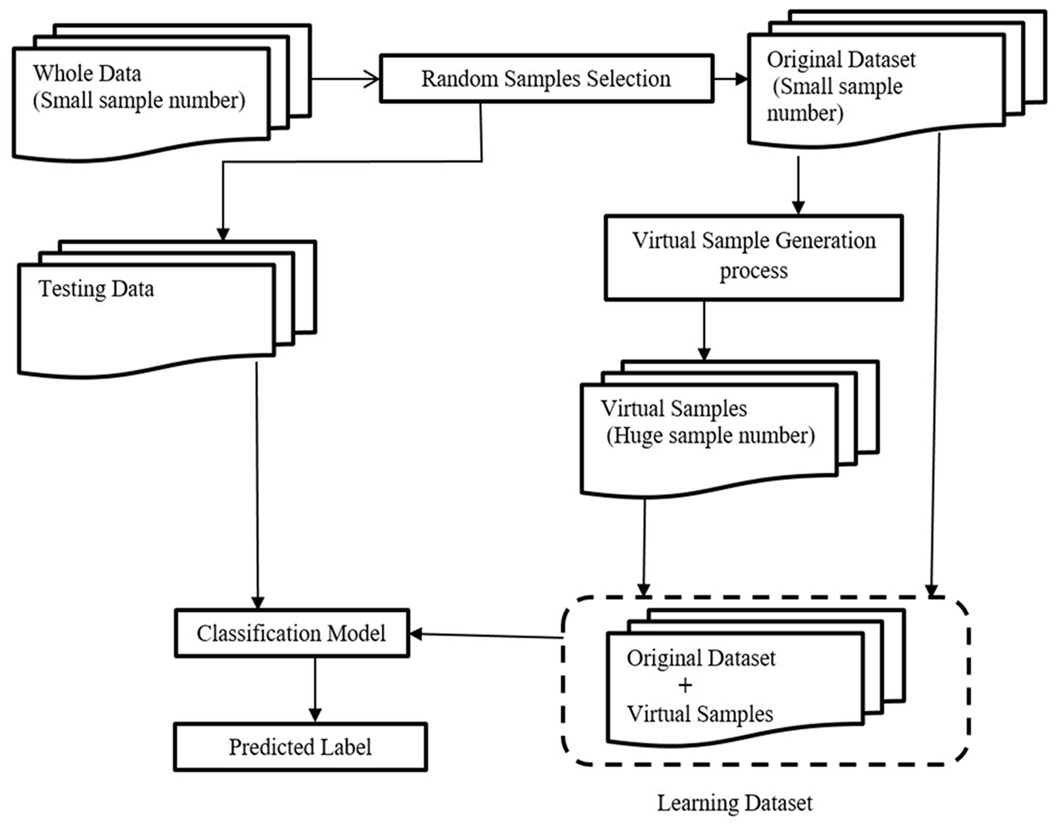
This section presents detailed steps to illustrate the method we developed in the present work, from data selection to the construction and generation of the virtual samples necessary to build the models and the classification tool. A schematic description of the whole procedure is shown in Figure 1. The procedure involved three steps: the first step was the selection of a small set of samples from a whole dataset; the second was the application of the VSG method to generate new samples; and the third step included data prediction and classification.
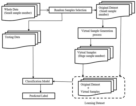
Figure 1.
Flowchart of the whole procedure with three different steps: (1) selection of a small sub-sample from the entire dataset and the remaining samples used as testing data; (2) application of the VSG method depending on the selected samples from the first step; (3) data prediction and classification.
The algorithm automatically ranked the top discriminative features and excluded the non-discriminative features. In the second step, a small set of samples was randomly selected, called selected samples, from the entire dataset, and the remaining samples were used as testing data. In the third step, we applied the proposed VSG method to generate new virtual samples, depending on the selected samples from the second step. Then, virtual samples were added to the selected samples for the next learning step. In the fourth step, the combined dataset (i.e., the original dataset plus the newly-generated virtual samples) was used to train the deep neural network, then we checked the classifier performance by classifying the testing data.
The first step of the proposed technique was to select samples randomly. These numbers were selected randomly from intervals of 3–10 as a small database for the first time; then, these numbers were set for all experiments to achieve comparisons. The number of randomly selected samples were 3, 5, 6, and 9. From each class, the Selected Samples (SS) were from the whole dataset (30 samples), and the remaining 24, 20, 18, and 12 samples, respectively, were the testing data.
The features of small selected samples of two different classes are represented in two matrices A and B with the same size as follows:
Let denote the indices of the rows of matrices A and B.
Let denote the indices of the column of matrices A and B.
Let a denote the value of the element A[i, j].
Let b denote the value of the element B[i, j].
The algorithm started by finding the following:
The minimum value for each feature in matrix A is NA. It appears as a single dimension matrix as follows:
The maximum value for each feature in matrix A is MA. It appears as a single dimension matrix as follows:
The mean value for each feature in matrix A is MeA. It appears as a single dimension matrix as follows:
The minimum value for each feature in matrix B is NB. It appears as a single dimension matrix as follows:
The maximum value for each feature in matrix B is MB. It appears as a single dimension matrix as follows:
The mean value for each feature in matrix B is MeB. It appears as a single dimension matrix as follows:
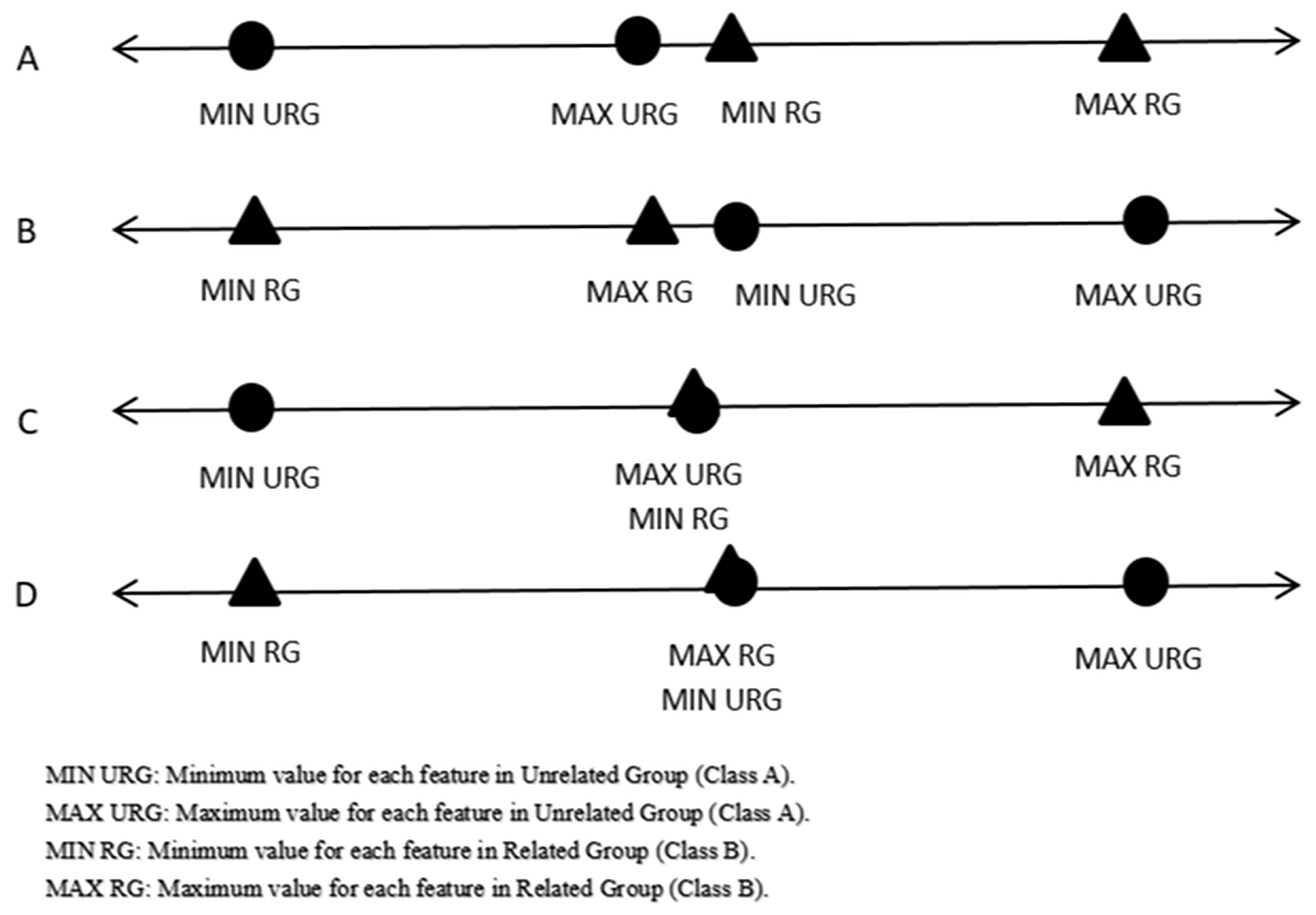
Then, for each iteration, starting from the first elements in the matrices NA, MA, NB, and MB to the last elements in these matrices, these four elements were the inputs of Equation (1) to check if there was any overlapping occurring in between them. If there was no overlap, then we expanded the intervals by Equations (5) and (6), otherwise, we tried to solve the overlaps by Equation (2).
The second process was the random variant generation to create new Virtual Samples (VS) based on the maximum, minimum, and mean calculated for every discriminative feature in each group in SS. After this, the virtual samples were added to SS by Equations (3) and (4). The number of generated samples could vary in terms of N (N = 10,000, 25,000, 50,000, 100,000, 200,000, and 300,000). All generated feature values were between the interval , while with a normal Gaussian distribution, the VS was generated by Equation (7).
The third step was the training phase of the system: SS and VS were employed as learning data and the residual data in the first step as testing data. Lastly, the classification performance was evaluated by using the Softmax classifier.
The proposed work can be summarized as follows: the new virtual samples were generated, depending on the original small dataset; the original dataset plus the newly-generated virtual samples both can be added to the training samples to expand the training dataset for machine learning significantly. Thus, our method can produce virtual samples closely related to the original datasets by applying a normal Gaussian distribution. The proposed work aims to make the classification model more stable and overcome the common limitations of the classification performance.
The working condition of the proposed system was that there were no overlaps between intervals. The system checked if the intervals had a direct ideal case, and the system started to generate a virtual sample without any pre-processing. Otherwise, the system tried to get rid of overlaps if success expanded the interval range, and it would start to generate virtual samples between the known intervals. Otherwise, it would skip to the next features.
3.1. Virtual Sample Generation Method
In the third step, for each discriminative feature, we applied the VSG method described in Algorithm 1 to generate virtual samples and then added them to the original dataset to produce a combined dataset for learning. The proposed method consisted of two parts. The first was the pre-processing technique, which searched for the rational interval (without overlaps) of each feature with the corresponding feature in another class. The second part was the random variant generation that increased the training dataset based on the original dataset for each rational feature. The code structure of the VSG method was as follows.
3.1.1. The Pre-Processing Method
The purpose of the pre-processing step was to preface the discriminative feature within the selected samples precisely. This step was mandatory in order to avoid overlapping of the sequence of corresponding discriminative features before generating new virtual samples. As an example, one of the datasets tested in this work included two groups: one Related Group (RG) including participants with autism spectrum disorders and an Unrelated Group (URG), which means healthy participants. It was clear that it was not reasonable to overlap the two different groups during the generation; therefore, this event was precluded by the pre-processing method as the following equations:
For each feature, its values are ordered in descending sort for class A in matrix MlsA, as follows:
For each feature, its values are ordered in ascending sort for class A in matrix mlsA, as follows:
For each feature, its values are ordered in descending sort for class B in matrix MlsB, as follows:
For each feature, its values are ordered in ascending sort for class B in matrix mlsB, as follows:
Here, Equation (2) tries to handle overlaps, and after each execution of this equation, it checks the ideal case.
If it succeeded to handle overlap (c < I), then Equations (5) and (6) were executed to expand the intervals, which were follow by Equation (7), which would be executed to generate N virtual features. Otherwise, the feature would be deleted and would not be taken into the consideration for generating virtual samples. Furthermore, the columns (features) in matrices A and B that failed to generate virtual numbers according to the previous Equation (2) would be deleted, and a new two matrices with new column dimension (H) would be generated NA and NB
H denotes the new number of the column of matrices NA and NB after deletion of unsuccessful columns (features) from matrices A and B, where .
In addition, the generated single dimension matrices and were combined horizontally into a single matrix NGA and NGB respectively, as shown in Equation (3).
N = number of virtual samples.
Finally, in Equation (4) combined vertically the NA with NGA matrices, and NB with NGB into a single matrices AA and BB respectively. These matrices (data) will be used as learning data for the classifier.
| Algorithm 1 The algorithm for virtual sample generation. |
| Input: Small number of samples as classes A and B. Output: Hundreds of thousands or millions of samples (N). 1: loop I = 1: number_ of_ features//number of columns in the matrix 2: {Find the Max, Min, and mean for each feature in classes A and B} 3: {Initialize MaxA = the maximum value in feature I in matrix A} 4: {Initialize MinA = the minimum value in feature I in matrix A} 5: {Initialize MeanA = the mean value for all values in feature I in matrix A} 6: {Initialize MaxB = the maximum value in feature I in matrix B} 7: {Initialize MinB = the minimum value in the feature I in matrix B} 8: {Initialize MeanB = the mean value for all values in feature I in matrix B} 9: If (MinA >= MaxB) or (MinB >= MaxA) //Ideal cases: see Figure 2 10: {If (MaxA > MaxB) //Expand the intervals before generating N virtual samples 11: MaxA = MaxA + MeanA 12: else 13: MaxB = MaxB + MeanB 14: if (MinA < MinB) //Expand the intervals 15: MinA = MinA − MeanA 16: else 17: MinB = MinB − MeanB} //Generate N virtual sample with a normal distribution as follows 18: VGA = MinA + (MaxA − MinA)*sum(rand(N, constant), 2)/constant; 19: VGB = MinB + (MaxB − MinB)*sum(rand(N, constant), 2)/constant; 20: else //Not ideal case: see Figure 3 21: call Algorithm 2 // The preprocessing 22: end loop 23: {New samples = small number of samples + N samples} |
The pre-processing technique primarily grouped samples based on their spatial relationship. The pre-processing algorithm can be summarized as follows:
Step 1: Find the maximum value, minimum value, and computed arithmetic mean for each feature for each class. Following this, check for any possible overlaps between the maximum values and minimum values for each feature in the first class with the corresponding feature in the second class. It is necessary to exclude possible overlaps (ideal cases, as can be noticed in Figure 2) before generating meaningful virtual samples.
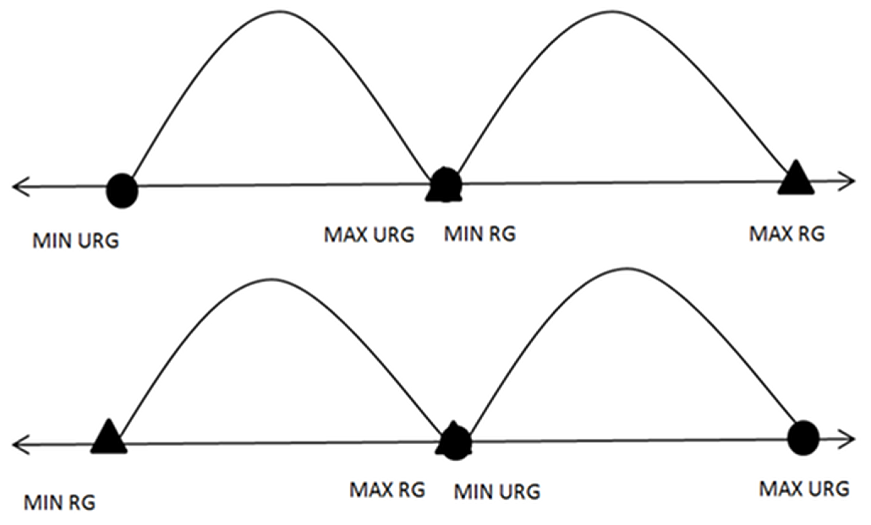
Step 2: After having verified the absence of overlaps, expand the sides using the mean for each feature and generating meaningful virtual samples based on a Gaussian distribution, as shown in Figure 4.
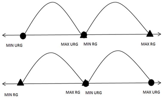
Figure 4.
Generating meaningful virtual samples based on a Gaussian distribution.
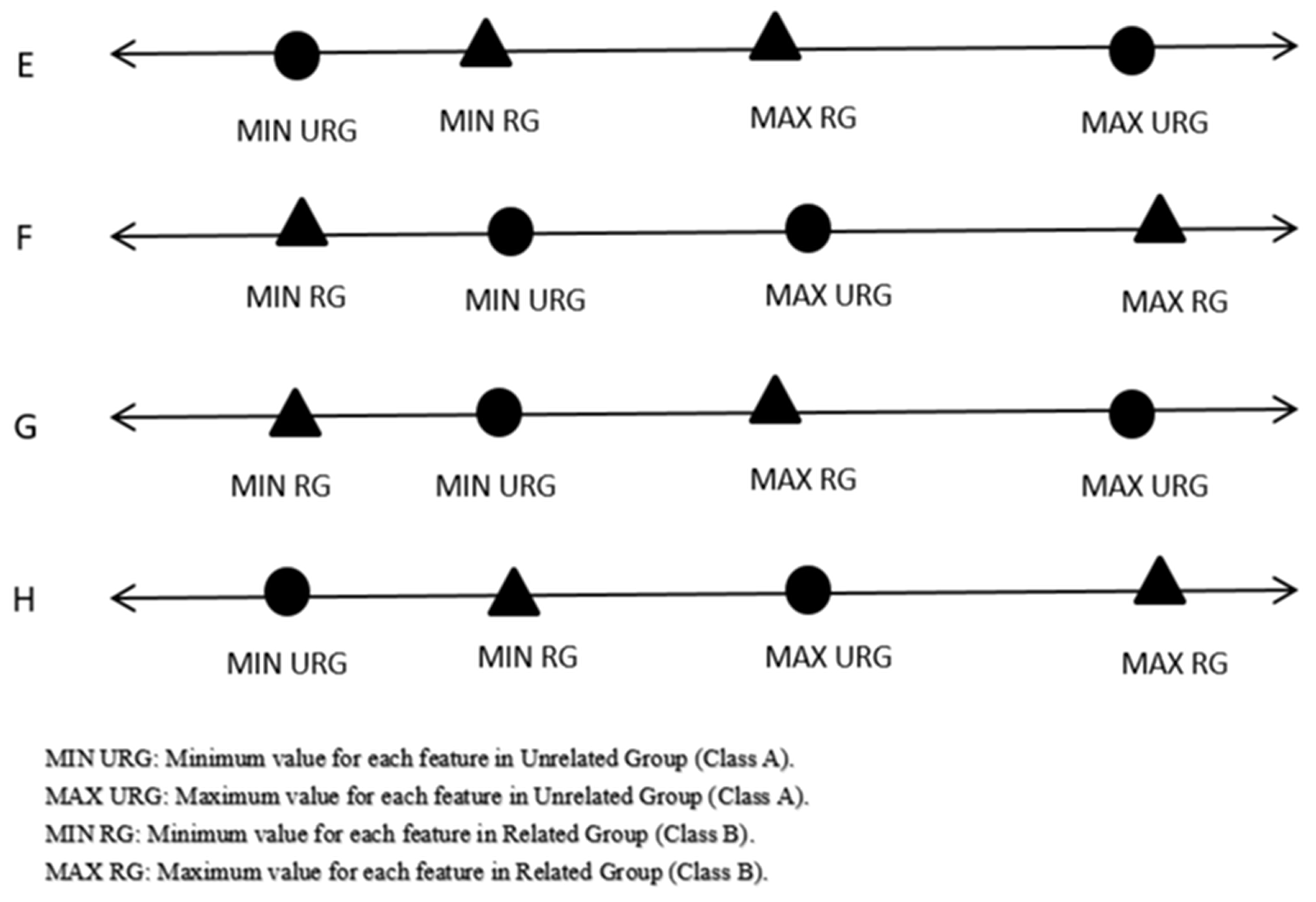
Step 3: In the case of overlaps, as in the case depicted in Figure 3 of the process, start removing overlaps by moving the points that are far from the mean.
Step 4: Repeat Steps 1–3 until removing all overlaps based on “Algorithm 2”. After this, the process generated virtual samples based on a Gaussian distribution, Equation (7).
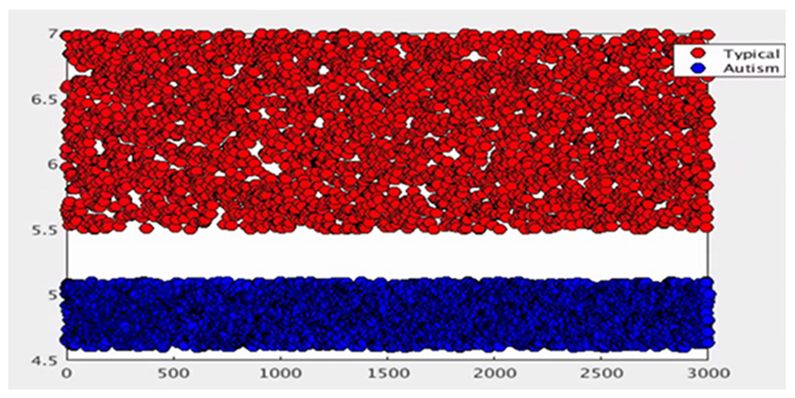
During this step, after the collections were formed using the pre-processing method for each discriminative feature, the mean and standard deviation for each group for all discriminative features were recalculated before moving to the next process. The distribution example of the virtual sample distribution after the pre-processing method is illustrated in Figure 5.
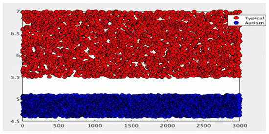
Figure 5.
Data distribution after preprocessing method.
| Algorithm 2 is the algorithm for solving overlapping. |
| Input: Feature with overlapping} // A and B are two different classes// Output: Feature without overlapping 1 :{Find the MaxA, MaxB, MinA, MinB, MeanA, and MeanB} 2 :{Initialize MlsA = the features in descending order for class A} 3 :{Initialize mlsA = the features in ascending order for class A} 4 :{Initialize MlsB = the features in descending order for class B} 5 :{Initialize mlsB = the features in ascending order for class B} 6 :{Initialize C = 1}// counter 7 : Loop until ((MinA >= MaxB) or (MinB >= MaxA))//Ideal case: Figure 2. 8 : {C = C + 1 9 : if (MinA < MinB and MaxB < MaxA)//Case E: Figure 3. 10 : if (MeanA − MinA <= MaxA-MeanA) 11 : MinA = mlsA[C] 12 : else 13 : MaxA = MlsA[C] 14 : if (MinA > MinB and MaxB > MinA and MaxB < MaxA)//Case G: Figure 3. 15 :if (MeanA − MinA <= MaxB-MeanB) 16: MinA = mlsA[C] 17: else 18: MaxA = MlsA[C] 19:if (MinB > MinA and MaxA > MinB and MaxA < MaxB)//Case H: Figure 3. 20:if (MeanB − MinB <= MaxA-MeanA) 21: MinB = mlsB[C] 22: else 23: MaxB = MlsB[C] 24: if (MinB < MinA and MaxA < MaxB)//Case F: Figure 3. 25 : if (MeanB − MinB <= MaxB − MeanB) 26 : MinB = mlsB[C] 27 : else 28: MaxB = MlsB[C] 29: end loop 30:{Back to Algorithm 1} |
3.1.2. Random Virtual Generation Technique
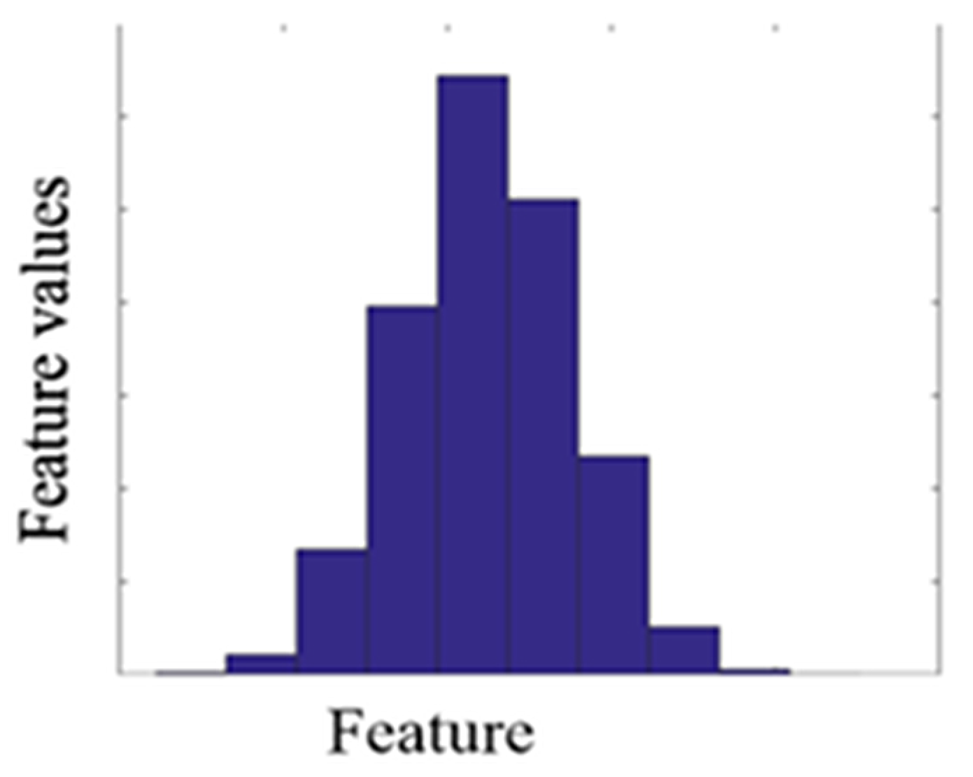
In the second process, Equation (7) generated new virtual samples depending on the maximum, minimum, mean, and standard deviation computed for every collection of all discriminative features and added them to the corresponding group of the original dataset Equations (3) and (4). A MATLAB function [33] was used to generate a virtual sample in a normal distribution. The distribution of the virtual sample is illustrated in Figure 6.
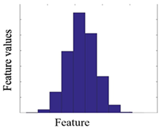
Figure 6.
Normal distribution for one feature after generating the virtual sample.
The Gaussian distribution is very widely used for distributions in probability, statistics, and many natural phenomena [34]. For example, heights, weight, blood pressure, the temperature during a year, and IQ scores follow a normal distribution. The Gaussian normal distribution is helpful because of the central limit theorem, which is a very important theorem in statistics. In addition, this was to avoid accumulation of all values in a few points only.
where:
X is a normal random variable.
is a mean.
is a standard deviation.
4. Experiment
4.1. Datasets
The above-described method was developed using a dataset provided by Scientific Institute IRCCSEugenio Medea. In addition, the proposed technique was tested with other available benchmark datasets.
The first dataset was collected at Scientific Institute IRCCS Eugenio Medea in Italy (Bosisio Parini, Italy). The dataset included data from 30 participants divided into two groups: 15 children with a clinical diagnosis of Autism Spectrum Disorder (ASD) (“ASD is a neurodevelopmental disorder characterised by persistent social impairment, communication abnormalities, and restricted and repetitive behaviours (DSM-5) (1, 2). ASD is a complex condition with an average prevalence of about 1% worldwide.”) and 15 participants with typical development. For each participant, 17 kinematic parameters (numerical features) related to an upper-limb movement were registered [35]. In the original work, a feature selection algorithm was used to identify the seven features that best differentiated participants with ASD from healthy controls. In the present work, our algorithm randomly selected six participants (from now on, samples) as an original small dataset, with three samples for each group (ASD and healthy children), and the remaining 24 samples were used as the testing dataset. For comparison, we generated 10,000 virtual samples using the proposed method for every collection in the first trial, and then, this rose by the following numbers each time: 25,000, 50,000, 100,000, 200,000, and 300,000. The identical learning procedure was repeated for five rounds.
The second dataset was the Escherichia coli dataset [30,36], and this included values of the measurements of E. coli bacteria (commonly found in the human gut). This dataset included 336 samples. Each sample belonged to one of eight classes, where each class referred to a type of E. coli bacteria. Each sample consisted of eight attributes; see the dataset description listed in Table 1. The training and testing set for this dataset were chosen as follows. We selected 77 samples for each of the first two classes (CPand IM) to ensure that we had binary classes with an equal sample number. Then, three samples were selected randomly from each of the selected class. These three samples represented the original small dataset. Starting from these three samples, the proposed method generated 10,000 virtual samples for every class for the first time. Then, the number of virtual samples were increased as follows: 25,000, 50,000, 100,000, 200,000, and 300,000 from each class. To give an example of this, the total number of training samples for the first round was 20,006 (six actual samples plus 20,000 virtual samples). The remaining 148 samples were used as testing data. After that, we repeated the experiment, randomly selecting five samples as an original small dataset, from each class of the E. coli dataset. Doing so, the total number of training samples was 10 plus the virtual samples. The remaining 144 samples were used as testing samples, and these steps were repeated five times.

Table 1.
Description of the three datasets.
The third dataset was the Breast Tissue dataset [36,37], and this included values of the measurements relative to the electrical impedance of freshly-excised tissue from the breast. This dataset included 106 samples where each sample belonged to one of six classes. Six classes of freshly-excised tissue were studied using electrical impedance measurements: carcinoma, fibroadenoma, mastopathy, glandular, connective, and adipose. The training and the testing set for this dataset were chosen as follows. We selected 15 samples for each of the first two classes (carcinoma and fibroadenoma) to ensure that we had binary classes with an equal samples number. Then, three samples were selected randomly from each of the selected classes. These three samples represented the original small dataset. Starting from these three samples, the proposed method generated 10,000 virtual samples for every class for the first time. Then, the number of virtual samples were increased as follows: 25,000, 50,000, 100,000, 200,000, and 300,000 from each class. To give an example of this, the total number of training samples for the first round was 20,006 (six actual samples plus 20,000 virtual samples). The remaining 24 samples were used as testing data. After that, we repeated the experiment, randomly selecting five samples as an original small dataset, from each class of the breast tissue dataset. Doing so, the total number of training samples was 20 plus the virtual samples. The remaining 20 samples were used as testing samples. These steps were repeated five times.
4.2. Classification Techniques
In this study, a deep neural network was implemented with a stacked auto-encoder, using the MATLAB Neural Network ToolboxTM auto-encoder functionality [38] for training a deep neural network and to classify an ASD. In more detail, a stacked auto-encoder is a neural network composed of various layers of sparse auto-encoders where the outputs of each layer are connected to the inputs of the sequential layers.
For classification, we used Softmax, which is a layer located in the top layer of the fully-connected layer network. Its non-linearity predicts the probability distribution over classes that have been given the input sentence [38,39]. Details of the Softmax method were described in [40]. In the present work, we applied Softmax to validate and evaluate the performance of our newly-proposed method.
In a neural network, it is not feasible to determine the goodness of the network topology only on the basis of the number of inputs and outputs [40]. Usually, a neural network must be empirically specified, selecting a model and determining the hidden layer quantity with the minimum validation error among multiple variants of the models [40]. Our first experiment was implemented by using a deep learning network with 100 hidden nodes in each layer. In the second experiment, we reduced the number of hidden nodes to 50, whereas in the third experiment, the first layer included 100 hidden nodes and the second layer 50 hidden nodes. This procedure was carried out for investigating the effect of hidden node size in the deep learning network. We continued until we obtained satisfactory results. The best performance was 100 hidden nodes in the first layer and 50 hidden nodes in the second layer.
5. Experimental Results
This section presents the results of the experiments on the three datasets (IRCCS Medea, E. coli, and Breast Tissue) in detail, for each dataset.
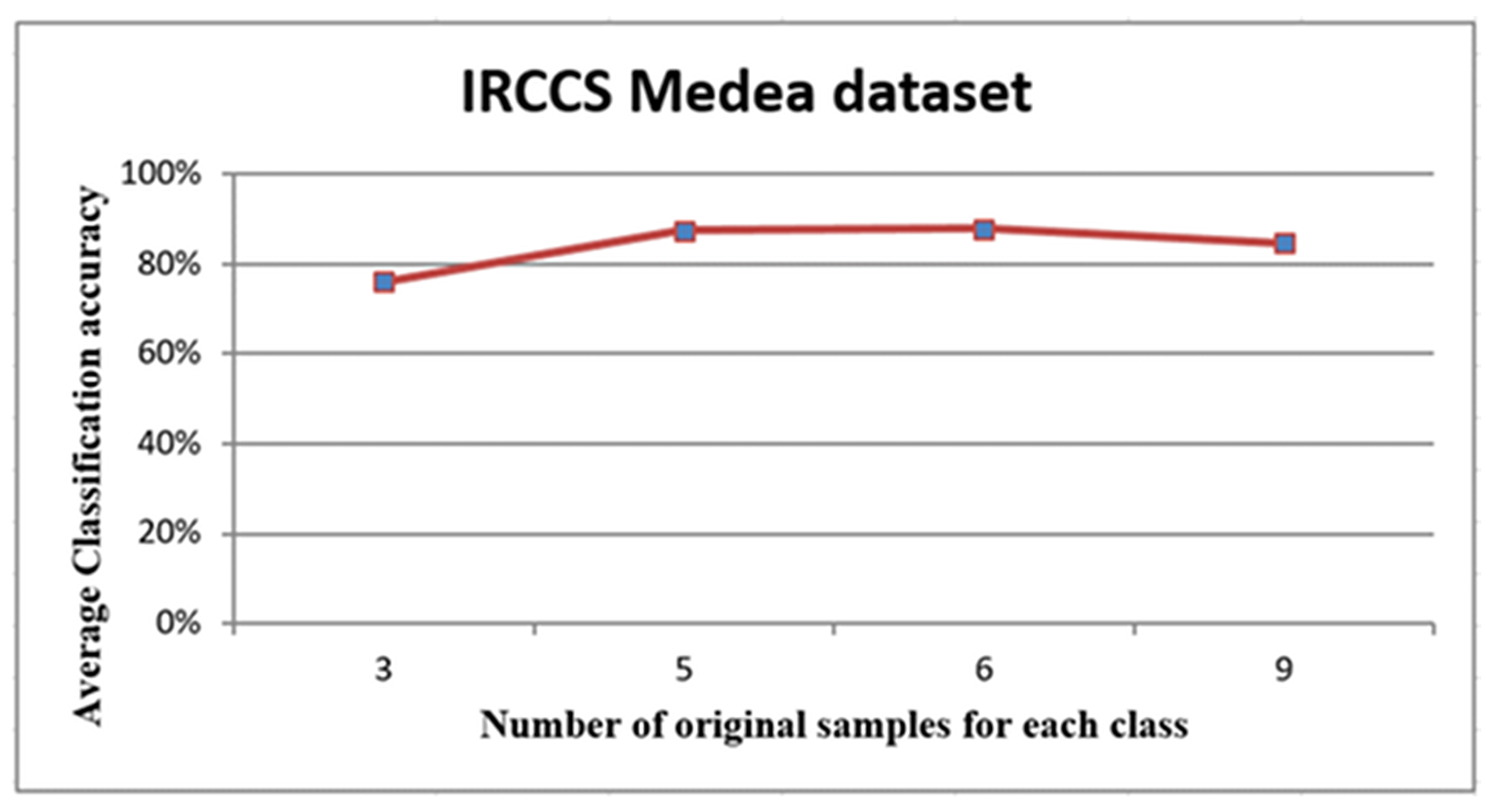
For the IRCCS Medea dataset, the averages accuracies are shown in Figure 7, Figure 8 and Figure 9 and listed in Table 2.
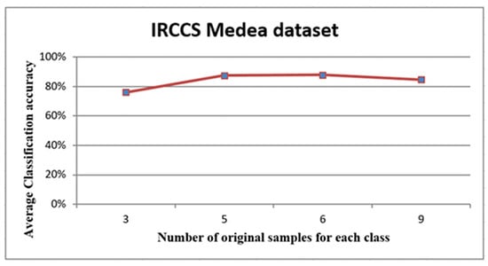
Figure 7.
The curve of the average accuracies of the simulated datasets.
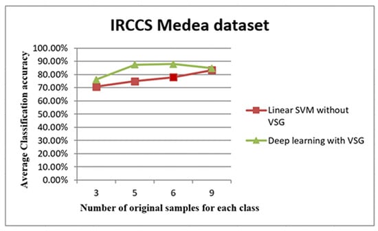
Figure 8.
The trend of average accuracy using the IRCCS dataset. The line graph in Figure 8 shows the comparison between the performance of linear SVM without Virtual Sample Generation (VSG) and deep learning with the VSG number in the IRCCS Medea dataset. The x-axis of this graph shows the original samples for each class that were used to generate the virtual sample in deep learning and the training sample for linear SVM, while the average of the classification accuracy is the y-axis.
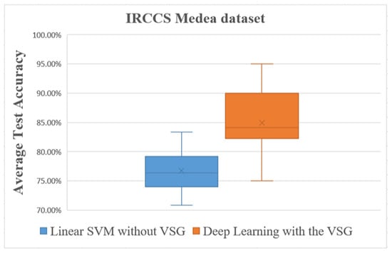
Figure 9.
Overall comparisons of the experimental results using the IRCCS Medea dataset.

Table 2.
The results of the average accuracy using the IRCCS Medea dataset.
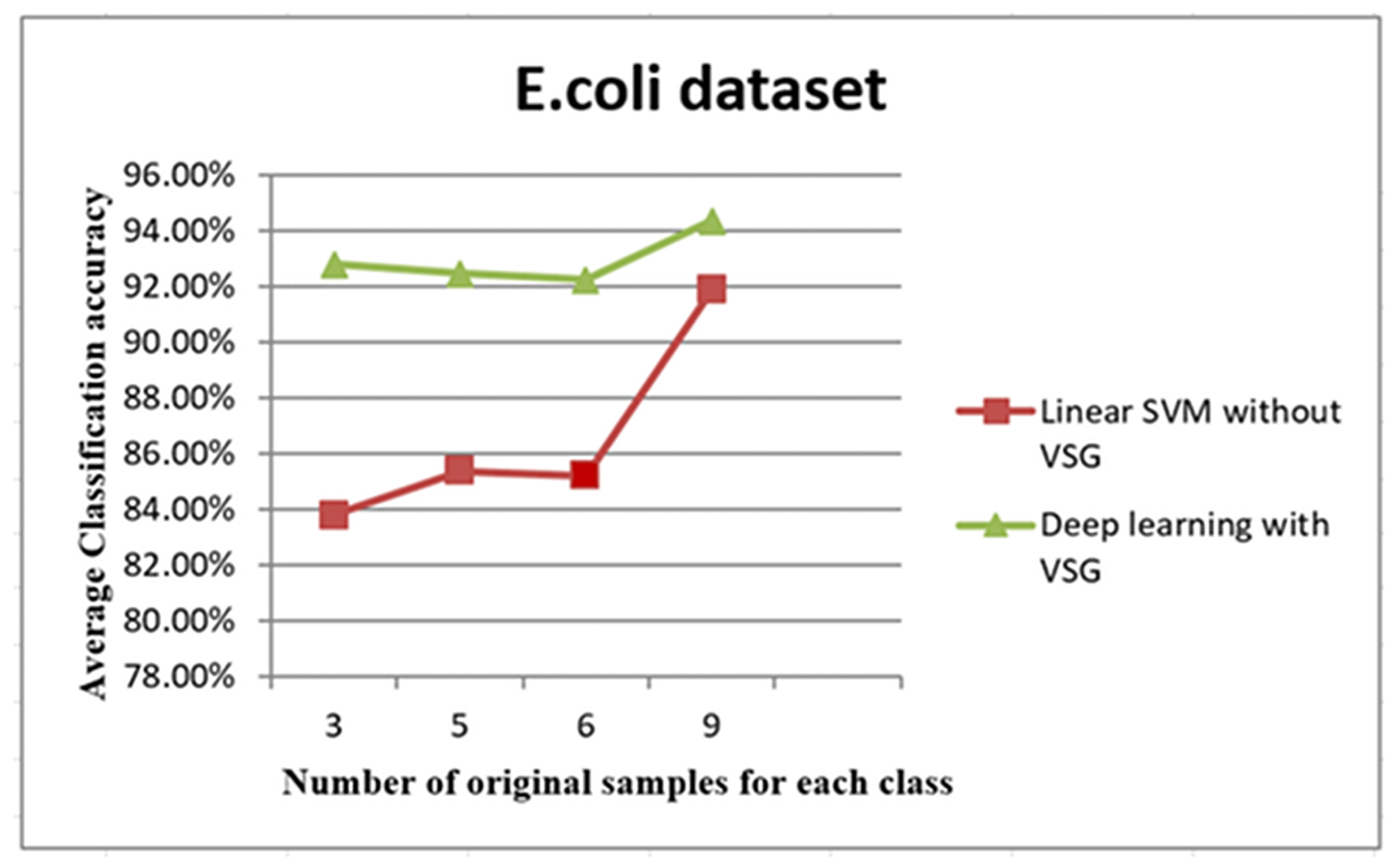
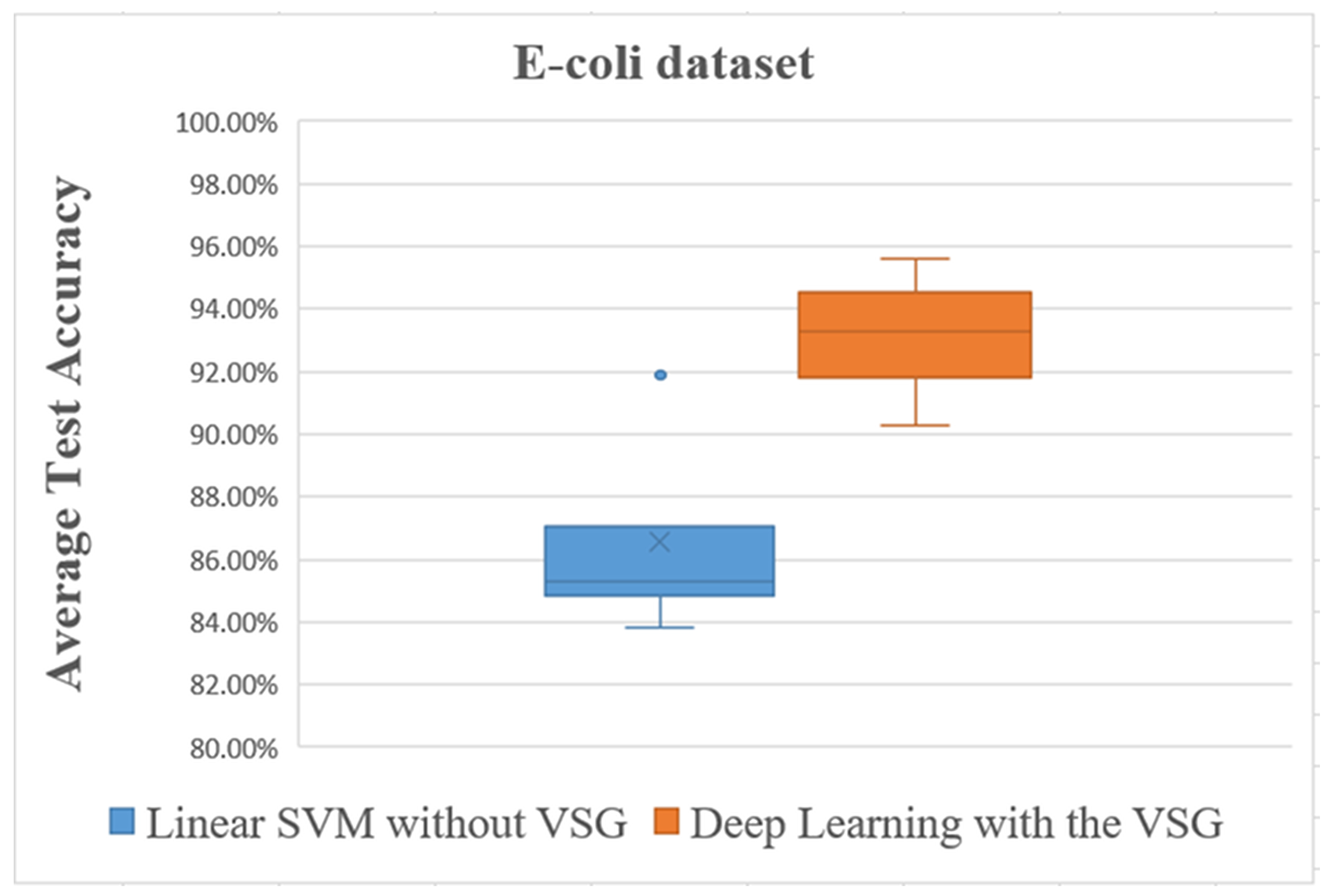
For the E. coli dataset, the average accuracies are shown in Figure 10 and Figure 11 and are listed in Table 3.

Figure 10.
The trend of average accuracy using the E. coli dataset. The x-axis of this graph shows the original samples for each class that were used to generate the virtual sample in deep learning and the training sample for linear SVM, while the average of classification accuracy is the y-axis.

Figure 11.
Overall comparisons of experimental results using the E. coli dataset.

Table 3.
The results of the average accuracy using the E. coli dataset.
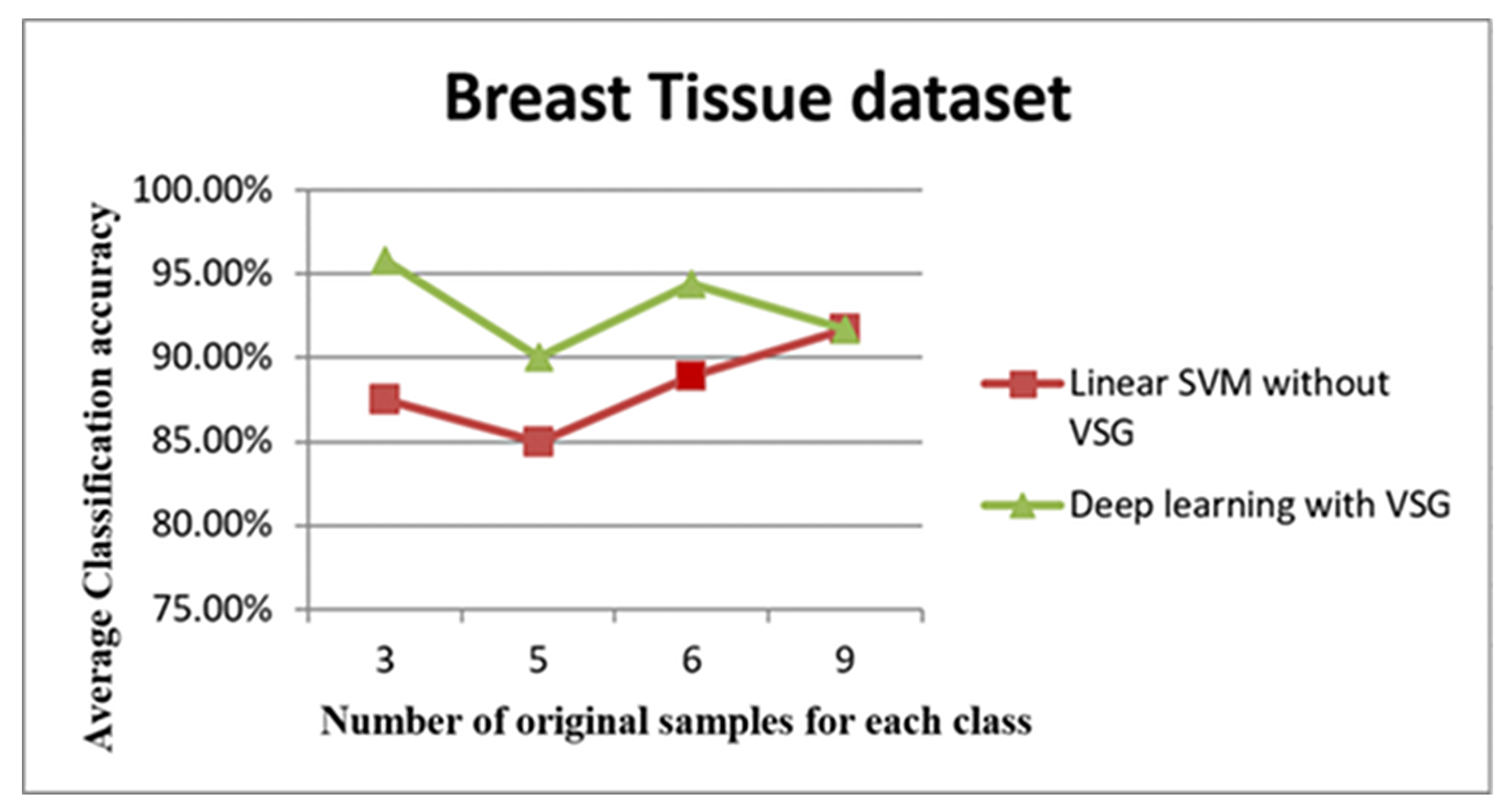
The third dataset was the Breast Tissue dataset. The average accuracies after performing these steps are shown in Figure 12 and Figure 13 and listed in Table 4.

Figure 12.
The trend of the average accuracy using the Breast Tissue dataset. The x-axis of this graph shows the original samples for each class that were used to generate the virtual sample in deep learning and the training sample for linear SVM, while the average of classification accuracy is the y-axis.
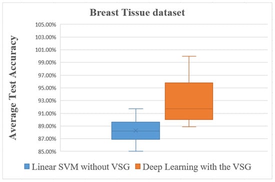
Figure 13.
Overall comparisons of the experimental results using the Breast Tissue dataset.

Table 4.
The results of the average accuracy using the Breast Tissue dataset.
The graph in Figure 7 depicts the relationship between the number of original samples for each class that was used to generate the virtual sample and the average of classification accuracy. The graph showed a growth in the relationship between six samples, followed by a levelling out. Overall, from this graph, it is possible to conclude that the number of original samples was not critical for generating the virtual sample. Moreover, this demonstrated that the proposed method was efficient with only a small number of original samples.
The plot depicted in Figure 8 shows distinctly that the present deep learning method with the proposed method exceeded in the first three intervals the linear Support Vector Machine method (SVM) used in [35]. In the 3, 5, and 6 samples, the “proposed method showed better results in terms of classification performance when using limited sample size compared to traditional linear SVM.”
The box plot in Figure 9 shows distinctly that the present deep learning method with the proposed method exceeded in overall comparisons the linear SVM method using the IRCCS Medea dataset.
The line graph in Figure 10 shows the comparison between the performance of linear SVM without VSG and deep learning with VSG number in the E. coli dataset. The experiment of our method performed on the E. coli dataset replicated the trend of findings for the IRCCS Medea dataset. Indeed, it was clear that deep learning with the proposed method outperformed the linear SVM method without VSG for the first of all intervals considered.
The box plot in Figure 11 shows distinctly that the present deep learning method with the proposed method exceeded in overall comparisons the linear SVM method using the E. coli dataset.
The line graph in Figure 12 shows the comparison between the performance of linear SVM without VSG and deep learning with VSG in the Breast Tissue dataset. The experiment of our method performed on the Breast Tissue dataset replicated the trend of the findings for the IRCCS Medea dataset and the E. coli dataset. Indeed, it is clear that deep learning with the proposed method outperformed the linear SVM method without VSG for the first three intervals considered.
The box plot in Figure 13 shows distinctly that the present deep learning method with the proposed method exceeded in overall comparisons the linear SVM method using the Breast Tissue dataset.
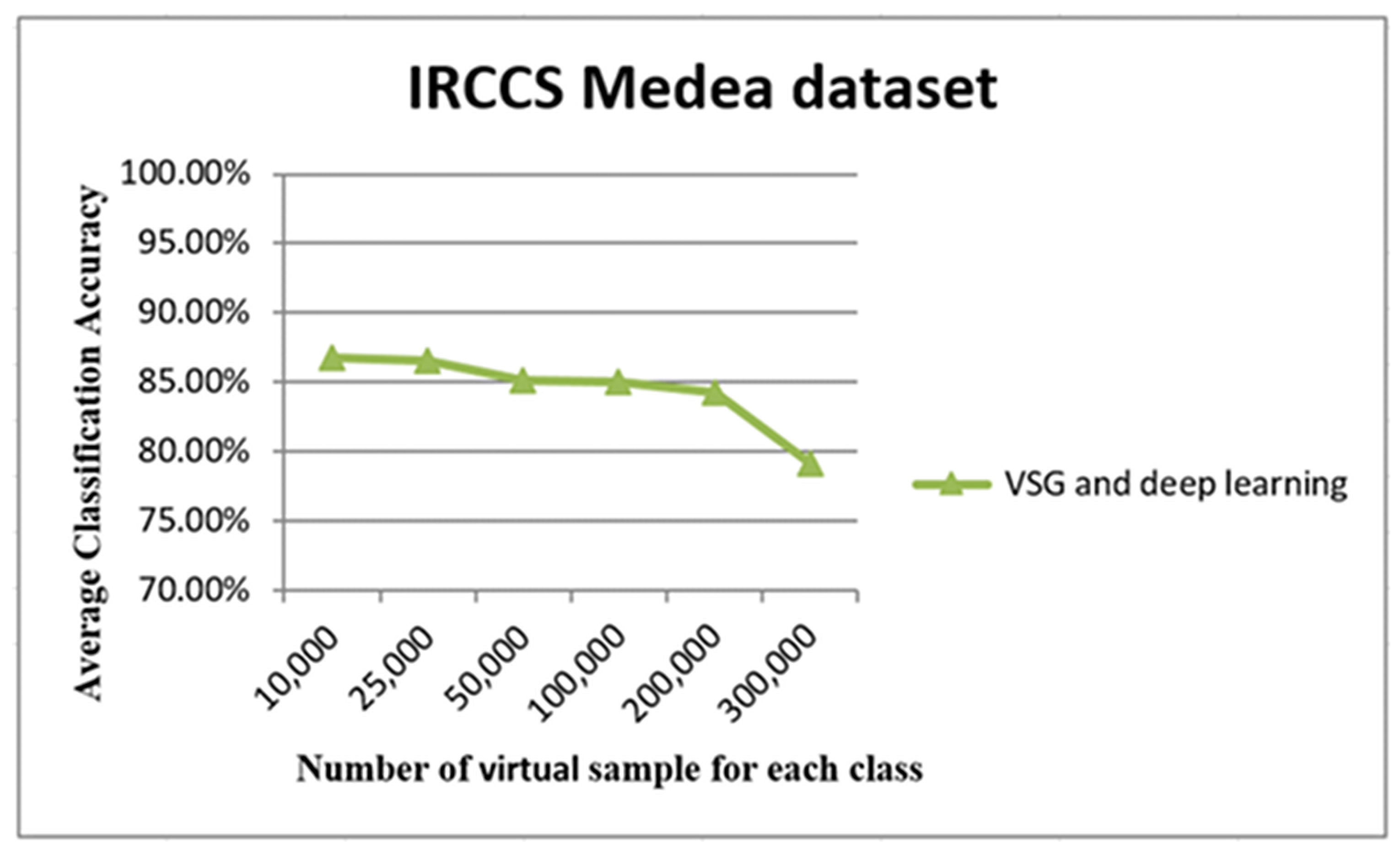
The graph in Figure 14 shows the relationship between the number of virtual samples (five original samples were used to generate these samples) and the average of classification accuracy. It may be seen clearly that average accuracy reached a peak with 25,000 samples. The accuracy performance remained adequately stable until 200,000 samples; then, a loss of accuracy was observed for 300,000 samples.
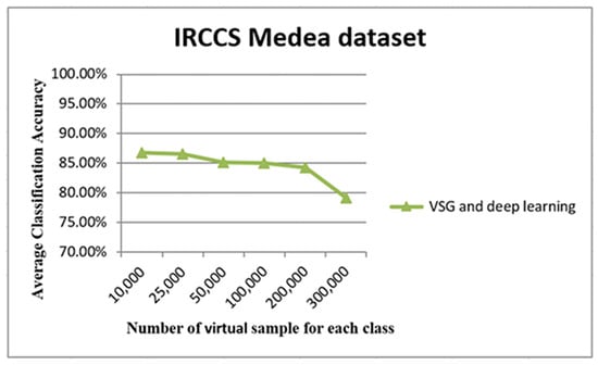
Figure 14.
The accuracy using only the original five small training IRCCS Medea datasets. The x-axis of this graph shows the number of virtual samples, while average accuracy appears on the y-axis.
6. The Numerical Example
In this section, we provide a numerical example to explain the proposed method, i.e., “the proposed method simulation.” Five samples from both classes A and B are shown in Table 5 and Table 6, respectively. Then, the maximum and minimum values were extracted, and the mean values were calculated from the first five features in both classes shown in Table 7, Table 8 and Table 9, respectively.

Table 5.
Five samples from the first class (A).

Table 6.
Five samples from the first class (B).

Table 7.
The maximum values extracted from the first five features.

Table 8.
The minimum values extracted from the first five features.

Table 9.
The mean values calculated from the first five features.
Features 1, 3, and 4 represented ideal cases, where we expanded the intervals and started to generate virtual random numbers based on a Gaussian distribution without any pre-processing, but Feature 2 was case H, so we performed a preprocessing before generating random numbers. In case H, to convert it to the ideal case, the MaxB or MinA would be changed depending on this simple comparison.
If (MeanA − MinA > MaxB − MeanB)
MinA = next position in the list, which is sorted in ascending order;
Else
MaxB = next position in the list, which is sorted in descending order;
End
The condition is false (3.28 - 3 > 3.2 - 2.92), so MaxB = 3.1;
Check that the case is still not the ideal case; it is a case H;
Check the same condition;
It is true now, so MinA = 3.1;
Check that the case is an ideal condition to expand the interval and start to generate virtual random numbers based on a Gaussian distribution as shown in Table 10 and Table 11.

Table 10.
Ten virtual samples (A).

Table 11.
Ten virtual samples (B).
7. Conclusions and Future Extensions
Deep neural networks are successful learning tools for building nonlinear models; however, they display unstable performance when using small datasets. In order to solve this issue, the present work proposed a new technique to generate virtual samples, starting from the original small dataset, which can be added to the original samples to expand the training dataset significantly for machine learning. Thus, our method can produce meaningful virtual samples closely related to the original datasets in order to make the learning phase more stable and overcome the common limitations of the classification performance, such as the limited size of clinical sample data.
The newly-developed technique focused on binary classification. However, this technique can also be used for multi-class data to generate virtual samples. In the case of multi-class data, the only condition needed would be that intervals must not overlap. Apart from this, the remaining procedure would be the same as for binary classification.
As just mentioned, our method required not having overlaps between intervals. The system checked if the intervals had a direct ideal case (Figure 2), then the system started generating a virtual sample without any pre-processing. Otherwise, the system tried to get rid of overlaps if success expanded the interval range, and it would start to generate virtual samples between the known intervals. Otherwise, it would skip to the next features. Therefore, the novel technique was easy to apply and could help to make the learning stage more stable and enhance the classification performance.
The application of our method to the IRCCS Medea and UCI datasets showed that the present technique could significantly improve the classification accuracy in cases where the dataset had a limited size. More specifically, when applied to the IRCCS Medea dataset, our method augmented the classification accuracy from 84.9 [35] to 95%, 83.8%–93.9% for only three samples in each class for the E. coli dataset, and from 91.7%–100% for the Breast Tissue dataset.
These findings demonstrated that our technique not only offered high classification accuracy, but was also reliable and easy to apply (refer to Algorithms 1 and 2). The experiments reported in this study also showed that, given an appropriate number of the generated virtual samples, the generalization efficiency of the classification on the new training set may be better than that of the original training set, and this agrees with many studies such as [34].
Future studies might delineate more specific matters in determining the best number for the original sample and the virtual sample in order to get maximum accuracy in terms of the results. In addition, the technique could be applied to a wide dataset to determine the strengths and limitations. These suggested directions could help to ensure that this important methodology is further and enhanced.
Author Contributions
M.W. conducted all experiments, analyses the results and wrote the first draft of the manuscript, A.C. provided data for the RCCSMedea dataset and revised the manuscript in each stage, A.A.-J. substantially contributed to the conception and design of the study, supervised and provided critical revision of the article. All authors reviewed the final manuscript.
Funding
The authors received no financial support for the research, authorship, and/or publication of this article.
Acknowledgments
The authors acknowledge Scientific Institute IRCCS Eugenio Medea in Italy for providing access to the database regarding the kinematic analysis of upper-limb movement in children with ASD and typically developing children. Crippa was supported by grants from the Italian Ministry of Health (GR-2011-02348929 and RICERCA CORRENTE 2018).
Conflicts of Interest
The authors declare no conflict of interest.
References
- LeCun, Y.; Bengio, Y.; Hinton, G. Deep learning. Nature 2015, 521, 436–444. [Google Scholar] [CrossRef] [PubMed]
- Deng, L.; Yu, D. Deep learning: Methods and applications. Found. Trends® Signal Process. 2014, 7, 197–387. [Google Scholar] [CrossRef]
- Charalambous, C.C.; Bharath, A.A. A data augmentation methodology for training machine/deep learning gait recognition algorithms. arXiv 2016, arXiv:1610.07570. [Google Scholar]
- Masood, A.; Al-Jumaily, A. Semi-advised learning model for skin cancer diagnosis based on histopathalogical images. In Proceedings of the 2016 38th Annual International Conference of the IEEE Engineering in Medicine and Biology Society (EMBC), Orlando, FL, USA, 16–20 August 2016; pp. 631–634. [Google Scholar]
- Li, D.C.; Wen, I.H. A genetic algorithm-based virtual sample generation technique to improve small data set learning. Neurocomputing 2014, 143, 222–230. [Google Scholar] [CrossRef]
- Strauss, K.A.; Puffenberger, E.G.; Morton, D.H. Maple syrup urine disease. J. Pediatr. 2013, 132, 17S–23S. [Google Scholar]
- Fu, Q.; Cao, J.; Renner, J.B.; Jordan, J.M.; Caterson, B.; Duance, V.; Luo, M.; Kraus, V.B. Radiographic features of hand osteoarthritis in adult Kashin-Beck Disease (KBD): The Yongshou KBD study. Osteoarthr. Cartil. 2015, 23, 868–873. [Google Scholar] [CrossRef][Green Version]
- Radiology, E.S. Medical imaging in personalised medicine: A white paper of the research committee of the European Society of Radiology (ESR). Insights Imaging 2015, 6, 141–155. [Google Scholar]
- Colubri, A.; Silver, T.; Fradet, T.; Retzepi, K.; Fry, B.; Sabeti, P. Transforming clinical data into actionable prognosis models: Machine-learning framework and field-deployable app to predict outcome of Ebola patients. PLoS Negl. Trop. Dis. 2016, 10, e0004549. [Google Scholar] [CrossRef]
- Vymetal, J.; Skacelova, M.; Smrzova, A.; Klicova, A.; Schubertova, M.; Horak, P.; Zadrazil, J. Emergency situations in rheumatology with a focus on systemic autoimmune diseases. Biomed. Pap. Med Fac. Palacky Univ. Olomouc 2016, 160, 20–29. [Google Scholar] [CrossRef]
- Ildstad, S.T.; Evans, C.H. Small Clinical Trials: Issues and Challenges; National Academy Press: Washington, DC, USA, 2001. [Google Scholar]
- Orru, G.; Pettersson-Yeo, W.; Marquand, A.F.; Sartori, G.; Mechelli, A. Using support vector machine to identify imaging biomarkers of neurological and psychiatric disease: A critical review. Neurosci. Biobehav. Rev. 2012, 36, 1140–1152. [Google Scholar] [CrossRef]
- Wedyan, M.; Al-Jumaily, A. Early diagnosis autism based on upper limb motor coordination in high risk subjects for autism. In Proceedings of the 2016 IEEE International Symposium on Robotics and Intelligent Sensors (IRIS), Tokyo, Japan, 17–20 December 2016; pp. 13–18. [Google Scholar]
- Wedyan, M.; Al-Jumaily, A. Upper limb motor coordination based early diagnosis in high risk subjects for Autism. In Proceedings of the 2016 IEEE Symposium Series on Computational Intelligence (SSCI), Athens, Greece, 6–9 December 2016; pp. 1–8. [Google Scholar]
- Li, D.C.; Wu, C.S.; Tsai, T.I.; Lina, Y.S. Using mega-trend-diffusion and artificial samples in small data set learning for early flexible manufacturing system scheduling knowledge. Comput. Oper. Res. 2007, 34, 966–982. [Google Scholar] [CrossRef]
- Huang, C.; Moraga, C. A diffusion-neural-network for learning from small samples. Int. J. Approx. Reason. 2004, 35, 137–161. [Google Scholar] [CrossRef]
- Khot, L.; Panigrahi, S.; Woznica, S. Neural-network-based classification of meat: Evaluation of techniques to overcome small dataset problems. Biol. Eng. Trans. 2008, 1, 127–143. [Google Scholar] [CrossRef]
- Li, D.C.; Chen, C.C.; Chang, C.J.; Lin, W.K. A tree-based-trend-diffusion prediction procedure for small sample sets in the early stages of manufacturing systems. Expert Syst. Appl. 2012, 39, 1575–1581. [Google Scholar] [CrossRef]
- Khot, L.R.; Panigrahi, S.; Doetkott, C.; Chang, Y.; Glower, J.; Amamcharla, J.; Logue, C.; Sherwood, J. Evaluation of technique to overcome small dataset problems during neural-network based contamination classification of packaged beef using integrated olfactory sensor system. LWT Food Sci. Technol. 2012, 45, 233–240. [Google Scholar] [CrossRef]
- Li, D.C.; Chen, L.S.; Lin, Y.S. Using functional virtual population as assistance to learn scheduling knowledge in dynamic manufacturing environments. Int. J. Prod. Res. 2003, 41, 4011–4024. [Google Scholar] [CrossRef]
- Li, D.C.; Yeh, C.W. A non-parametric learning algorithm for small manufacturing data sets. Expert Syst. Appl. 2008, 34, 391–398. [Google Scholar] [CrossRef]
- Chao, G.Y.; Tsai, T.I.; Lu, T.J.; Hsu, H.C.; Bao, B.Y.; Wu, W.Y.; Lin, M.T.; Lu, T.L. A new approach to prediction of radiotherapy of bladder cancer cells in small dataset analysis. Expert Syst. Appl. 2011, 38, 7963–7969. [Google Scholar] [CrossRef]
- Li, D.C.; Lin, Y.S. Using virtual sample generation to build up management knowledge in the early manufacturing stages. Eur. J. Oper. Res. 2006, 175, 413–434. [Google Scholar] [CrossRef]
- Johnson, R.; Wichern, D. The multivariate normal distribution. In Applied Multivariate Statistical Analysis; Prentice-Hall Inc.: Englewood Cliffs, NJ, USA, 1982; pp. 150–173. [Google Scholar]
- Scott, P.D.; Wilkins, E. Evaluating data mining procedures: Techniques for generating artificial data sets. Inf. Softw. Technol. 1999, 41, 579–587. [Google Scholar] [CrossRef]
- Khot, L.R. Characterization and Pattern Recognition of Selected Sensors For Food Safety Applications; North Dakota State University: Fargo, ND, USA, 2009. [Google Scholar]
- Li, D.C.; Liu, C.W.; Chen, W.C. A multi-model approach to determine early manufacturing parameters for small-data-set prediction. Int. J. Prod. Res. 2012, 50, 6679–6690. [Google Scholar] [CrossRef]
- Niyogi, P.; Girosi, F.; Poggio, T. Incorporating prior information in machine learning by creating virtual examples. Proc. IEEE 1998, 86, 2196–2209. [Google Scholar] [CrossRef]
- Li, D.C.; Fang, Y.H.; Lai, Y.Y.; Hu, S.C. Utilization of virtual samples to facilitate cancer identification for DNA microarray data in the early stages of an investigation. Inf. Sci. 2009, 179, 2740–2753. [Google Scholar] [CrossRef]
- Dheeru, D.; Karra Taniskidou, E. UCI Machine Learning Repository. 2017. Available online: http://archive.ics.uci.edu/ml/datasets.php (accessed on 25 November 2019).
- Liu, Y.; Zhou, Y.; Liu, X.; Dong, F.; Wang, C.; Wang, Z. Wasserstein GAN-Based Small-Sample Augmentation for New-Generation Artificial Intelligence: A Case Study of Cancer-Staging Data in Biology. Engineering 2019, 5, 156–163. [Google Scholar] [CrossRef]
- Martin, C.; Springate, C. Synthetic Sample Generation Representing the English Population Using Spearman Rank Correlation and Chomsky Decomposition. Value Health 2018, 21, S221. [Google Scholar] [CrossRef]
- MathLab. Normally Distributed Random Numbers. 2018. Available online: https://www.mathworks.com/help/matlab/ref/randn.html (accessed on 25 November 2018).
- Yang, J.; Yu, X.; Xie, Z.Q.; Zhang, J.P. A novel virtual sample generation method based on Gaussian distribution. Knowl. Based Syst. 2011, 24, 740–748. [Google Scholar] [CrossRef]
- Crippa, A.; Salvatore, C.; Perego, P.; Forti, S.; Nobile, M.; Molteni, M.; Castiglioni, I. Use of Machine Learning to Identify Children with Autism and Their Motor Abnormalities. J. Autism Dev. Disord. 2015, 45, 2146–2156. [Google Scholar] [CrossRef]
- UCI. UCI Machine Learning Repository. 2017. Available online: http://archive.ics.uci.edu/ml/datasets.php (accessed on 25 November 2019).
- Lichman, M. UCI Machine Learning Repository. 2013. Available online: http://archive.ics.uci.edu/ml (accessed on 25 November 2019).
- MathLab. Train Stacked Autoencoders for Image Classification. 2017. Available online: https://www.mathworks.com/help/deeplearning/examples/train-stacked-autoencoders-for-image-classification.html (accessed on 25 November 2019).
- Kalchbrenner, N.; Grefenstette, E.; Blunsom, P. A convolutional neural network for modelling sentences. arXiv 2014, arXiv:1404.2188. [Google Scholar]
- Svozil, D.; Kvasnicka, V.; Pospichal, J. Introduction to multi-layer feed-forward neural networks. Chemom. Intell. Lab. Syst. 1997, 39, 43–62. [Google Scholar] [CrossRef]
© 2019 by the authors. Licensee MDPI, Basel, Switzerland. This article is an open access article distributed under the terms and conditions of the Creative Commons Attribution (CC BY) license (http://creativecommons.org/licenses/by/4.0/).


