Abstract
Home Healthcare (HHC) is an emerging and fast-expanding service sector that gives rise to challenging vehicle routing and scheduling problems. Each day, HHC structures must schedule the visits of caregivers to patients requiring specific medical and paramedical services at home. These operations have the potential to be unsuitable if the visits are not planned correctly, leading hence to high logistics costs and/or deteriorated service level. In this article, this issue is modeled as a vehicle routing problem where a set of routes has to be built to visit patients asking for one or more specific service within a given time window and during a fixed service time. Each patient has a preference value associated with each available caregiver. The problem addressed in this paper considers two objectives to optimize simultaneously: minimize the caregivers’ travel costs and maximize the patients’ preferences. In this paper, different methods based on the bi-objective non-dominated sorting algorithm are proposed to solve the vehicle routing problem with time windows, preferences, and timing constraints. Numerical results are presented for instances with up to 73 clients. Metrics such as the distance measure, hyper-volume, and the number of non-dominated solutions in the Pareto front are used to assess the quality of the proposed approaches.
1. Introduction
Home Healthcare (HHC) aims at supporting people with different degrees of dependencies to remain at home instead of receiving long-term care at a traditional medical institution. It encompasses a large variety of care provided at hospitals and gives rise to challenging planning and coordination problems. HHC is set to become an increasingly important issue in the years ahead with the longer human life expectancy. Research on these emerging problems has the intent to establish a fine coordination of human and material resources to provide an optimized planning that maximizes the quality of home healthcare while controlling logistics costs. Therefore, effective organization of HHC structures requires the use of optimization methods and decision support tools.
The aim in our study is to determine the routes to be performed by a fleet of vehicles (associated with a group of caregivers) available to serve a set of geographically-dispersed customers (corresponding to the patients), who have preferences associated with caregivers, and so that the activity is planned in the most effective way. The specificities rely on the fact that a home healthcare service must often be performed in a given time window and may require the intervention of several caregivers simultaneously. In addition, sometimes a patient needs several types of care linked by precedence constraints. These timing constraints impose the coordination of several caregivers. This problem is hence modeled as a variant of the vehicle routing problem called VRPTW-SP for the Vehicle Routing Problem with Time Windows, Synchronization, and Precedence constraints. In a previous work (Ait Haddadene et al. [1]), the minimization of the traveling cost and the sum of non-preferences related to customers were considered as a single-objective function. The obtained results showed the conflicting nature of these criteria, which is why, we are particularly interested in solving the bi-objective version of VRPTW-SP.
The problem at hand is an extension of the Vehicle Routing Problem (VRP), which is one of the most-studied combinatorial optimization problems. First introduced by Dantzig and Ramser [2], the aim of this NP-hard problem is to determine a set of minimal cost routes in which a set of customers is to be served by a fleet of vehicles based at a depot node. A detailed survey can be found in Toth and Vigo [3]. Currently, one of the most effective metaheuristics for the VRP is the hybrid genetic algorithm introduced by Vidal [4], which was latter generalized to solve more than 26 VRP variants.
Among the different classes of VRP, the VRP with Time Windows (VRPTW) stands as the basis variant of our studied problem. Heuristic and metaheuristic approaches have been widely used to solve the VRPTW such as those proposed by Kindervater and Savelsbergh [5], Bräysy and Gendreau [6], Nagata [7], and Bräysy et al. [8]. In the field of healthcare, most problems are modeled as a VRPTW. In fact, the origin of vehicle routing problems in HHC systems may be linked to the door-to door-transportation of elderly or disabled persons (Dial A Ride Problems (DARP)) proposed by Bodin and Sexton [9]. A few years later, this variant was extended to the Home Healthcare (HHC) problem by Cheng and Rich [10], where caregivers are assigned to patient homes to provide specific care. A mixed integer mathematical model was proposed, and a heuristic approach was developed. At this stage, the numerical results were given for only four caregivers and 10 patients.
Since then, many other studies were carried out, and they are classified in this paper according to: (1) optimization criterion, (2) constraints, and (3) solution approaches. For a more exhaustive review, see for instance [11,12].
Table 1 provides a classification of the main types of tackled objectives. Note that each category involves a broad class of possible objective functions. Table 2 summaries the criteria considered in the reviewed papers, these last being listed in Column 1. Columns 2–9 correspond to each of the objectives enumerated in Table 1. When a paper tackles one of the objectives, a symbol (×) is shown in the corresponding cell.

Table 1.
Common types of optimization criteria.
Table 2.
Optimization criteria found in the literature.
As shown in the last table, the objective of minimizing traveling costs, waiting costs, or patient preferences is undoubtedly the most widespread in the literature. However, when multiple objective functions are handled, they are often considered within a single criterion as a weighted sum.
Instead of being part of the objective function, some characteristics of a problem may sometimes be considered as constraints. In our study for instance, time is handled through time windows associated with patient care, as well as through interdependencies between the routes performed by caregivers. This interdependence is defined as operation synchronization in the classification suggested by Drexl [58]. More specifically, in the context of home healthcare, Labadie et al. [32] identified two kinds of synchronization:
- Simultaneous synchronization: A patient may request several caregivers at the same time. This is for example the case when a bath is requested by the patients, but more than one caregiver is needed to provide this service (because of a heavy load for example). This is called simultaneous synchronization, and it means that staff should start simultaneously (within a tight time lag) performing a given number of tasks or a specific type of care.
- Precedence synchronization: A patient can also request more ordered cares. This is the case when preparing a patient is necessary before care or another service (such as to be transported to a hospital).
Even if synchronization is common in real-life problems, it has not received a large amount of attention in comparison with other constraints. In fact, researches have been mainly focused on ensuring high service quality through constraints such as time windows and service types.
Table 3 presents the most common families of constraints taken into account in the HHC context, while Table 4 summarizes the constraints handled in the reviewed papers.
Table 3.
Common families of constraints.
Table 4.
Constraints found in the literature.
Table 4 shows that time windows and qualification are considered in the majority of the reviewed papers. However, some characteristics such as simultaneous synchronization, precedence synchronization, and periodicity have attracted less interest in the literature. To the best of our knowledge, only our previous works and that of [25] combine both types of synchronization constraints (simultaneous and precedence) in the same model.
Table 5 presents solution approaches that were used to solve the problems studied in the reviewed papers. These methods are classified into two general categories: exact approaches (Column 2) and heuristics/metaheuristics (Column 3).
Table 5.
Common solution approaches.
From this literature review on vehicle routing problems related to the HHC context, It can be seen that most of proposed methods are metaheuristics and that most of papers present a mathematical method (mixed integer linear program) by mean of solvers. Furthermore, the majority of studies involving different objectives considered an aggregated function defined as a weighted sum of the considered criteria. Indeed, in all these works, the multi-criteria issue was managed through a linear combination of the different objectives. The use of this kind of approach has well-known drawbacks: (a) finding the appropriate weights is not trivial; (b) multiple runs are needed to provide the decision maker with enough solutions; (c) non-supported solutions cannot be found whatever the selected weights.
Regarding vehicle routing problems, several authors have been interested in algorithms based on Pareto optimality to solve different combinatorial optimization problems. For example, Jozefowiez et al. [59] proposed a Non-dominated Sorting Genetic algorithm (NSGAII) for solving the vehicle routing problem with route balancing. In the same context, Lacomme et al. [60] tested several local search procedures within the NSGAII framework for the capacitated arc routing problem, and more recently, Velasco et al. [61] adapted this previous local search for solving the pick-up and delivery problem.
To the best of our knowledge, [38] and the more recent papers [51,52] are the only ones that consider the routing and planning problem in HHC as a multi-objective variant. In the first one, the compromise relations were between minimizing travel costs and maximizing the level of satisfaction of patients in home care structures. A metaheuristic based on multi-directional local search was proposed to build an approximated front. The latter was compared to the optimal Pareto front obtained by using an -constraint method. The study of [51] considered also a multicriteria problem with three objectives: (1) minimizing the total working time of the caregivers, (2) optimizing the quality of service by minimizing the patients time window and the synchronized visits non-satisfaction, (3) and minimizing the maximal working time difference among nurses and auxiliary nurses. To solve the problem, these authors designed a Memetic Algorithm for Multi-objective Optimization (MAMO), which uses an NSGAII structure combined with multi-directional local searches. In [52], a bi-objective optimization model aimed to make a tradeoff between transportation cost and environmental pollution. The authors proposed various versions of heuristics, metaheuristic, and modified/hybrid methods. Metaheuristics are simulated annealing and swarm algorithms. Their evaluation is made through four assessment metrics and the Pareto-optimal solutions of the employed metaheuristics by the epsilon constraint method.
Overall, it can be seen that most implementations can be found in the category of metaheuristics, and the majority of them use local search procedures. However, the papers [38,44,47,48,51] may be the only ones that proposed a population-based metaheuristic for solving a vehicle routing problem in the HHC field. In addition, only [38,51] tackled a multicriteria problem through this kind of solution approach.
The last trends seem to focus either on uncertainties or dynamic data ([62] studied a pick-up and delivery version of HHC with travel time uncertainty; [63] worked on the caregiver routing problem solved in a dynamic context with uncertainties and random events by a multi-agent system; [53] proposed a dynamic method to handle sudden incidents in practice; and [54] considered the dynamic arrival and departure of patients and nursing staff to solve the daily scheduling and routing problem in a long-term perspective). However, none of those dealt with multi-objective functions.
Summarizing the literature review, most works on vehicle routing problems raised in HHC, either considering simultaneous/precedence synchronization or not, have tackled the multi-criteria issue by a weighted sum of the considered criteria. The contribution of this paper is three-fold: (1) The most-used benchmark from Bredström and Rönnqvist [17] is handled under a bi-objective optimization, allowing another analysis of the trade-off between both the cost and the non-preference values, which tends to bring numerical results close to zero when using a weighted sum. (2) Population-based methods are designed to solve the bi-objective VRP with time windows, preferences, and timing constraints. (3) Several local search strategies are tested within the non-dominated sorting methods proposed here.
The remainder of this article is structured as follows: The problem definition is exposed in Section 2. The different component of the basic NSGAII are detailed in Section 3. Three algorithm designs are deduced from combining these components and are exposed in Section 4. The results of the proposed methods, tested on instances from the literature, are presented in Section 5. Finally, conclusion and future research direction are provided in Section 6.
2. Problem Definition
To model the studied problem, patients were associated with customers and caregivers with vehicles. The problem can be seen as a variant of the vehicle routing problem with a time window and specific synchronization constraints encountered in the home healthcare system. In particular, the problem at hand focuses on cases in which some patients may ask for some services requiring more than one caregiver with different skills to be accomplished, either simultaneously or in a given order.
Before explaining how simultaneous synchronization/precedence constraints and objective function are modeled, let us introduce the following notation:
- N is the set of customers.
- is the set of initial and final depots denoted as d and f, respectively.
- is the set of nodes.
- S is the set of offered services, where is the subset of services requested by customer .
- denotes the service time window at customer i, which are hard in this study. Indeed, service at customer i must start only in this interval: if a caregiver arrives at i before , a waiting time occurs, and the service after time is not allowed to be provided.
- K is the set of available vehicles, where is the subset of vehicles performing service .
- is the travel cost from customer to .
- is the non-preference value of customer to the caregiver .
- is a scheduling variable corresponding to the starting time of the service by vehicle k at customer .
- is equal to one if and only if the vehicle goes from i to j, zero otherwise.
VRPTW-SP consists of building a set of routes, such that the following conditions are satisfied:
- each route starts at the initial depot d and ends at the final depot f,
- each vehicle route does not exceed the maximal imposed duration,
- each customer time window must be respected,
- each customer service request is satisfied,
- each service must be accomplished by the qualified caregiver,
- timing constraints linking the start time of services at customers asking for more than one service must be considered.
In a preliminary work [1], the authors extended the constraints proposed by [32] to deal with both types of synchronization (simultaneous and precedence) while retaining the idea of avoiding node duplication for customers requiring synchronized visits. In addition, several heuristics and local research procedures were proposed to solve the problem as a single-objective variant. Here, we propose to use these methods to solve the bi-objective problem.
Synchronization constraints are expressed for some customers by defining as the required time between the starting times of services s and r requested by customer i. For a simultaneous pair of services, this gap is obviously set to zero. Then, synchronization/precedence constraints are defined as:
The considered objective function is formulated as follows:
with,
Here, Z is regarded as a two-dimensional vector , where both objectives must be optimized simultaneously. For more details on the proposed mathematical model, readers are referred to Ait Haddadene et al. [1] in which was minimized. Note that patient preference for caregivers is quantified by a negative value. Thus, a large negative value means a highly-desired assignment, while a positive value means an undesired visit.
3. Non-Dominated Sorting Genetic Algorithms
3.1. Motivation
The principle of the Non-Dominated Sorting Genetic Algorithm (NSGAII) proposed by [64] is chosen to solve the bi-objective VRPTW-SP, since it has been successfully used for solving multi-objective combinatorial optimization problems and especially vehicle routing problems, such as in Lacomme et al. [60], Velasco et al. [61], and Labadie et al. [65]. As far as we know, there are no works addressing the NSGAII to solve the multi-objective vehicle routing problems in the HHC context.
The remainder of this section is organized as follows: First, Section 3.2 introduces the non-trivial framework of NSGAII. Then, from Section 3.3, Section 3.4, Section 3.5 and Section 3.6, the adaptation to the bi-objective VRPTW-SP is described, while introducing new components. However, two new methods will be derived by combining these various proposed components such as a restart NSGAII, which generalizes the main idea of the NSGAII, and a so-called NSILS for The Non-Dominated Sorting Iterated Local Search, merging a non-dominated sorting concept with the iterated local search procedure. The general structures of these three methods will be detailed in Section 4.
3.2. General Principle
The proposed approaches work on a population of solutions and can be seen as an adaptation of the non-dominated sorting genetic algorithm (NSGAII). It is a Pareto-optimal method based on the dominance concept. Dominance relations in the Pareto sense are defined as follows: for two objectives and to be minimized, we say that a solution x dominates a solution y if . This lets us say that a solution is non-dominated, or is efficient if no solution can be found that improves strictly both objectives. In other terms, it is impossible to improve one of the objectives without deteriorating the other one.
The optimization in the Pareto sense computes the set of non-dominated solutions called the Pareto front. A non-dominated sorting uses a ranking method for the fitness assignment and a crowding distance for maintaining the diversity of the population.
In NSGAII, successive generations of solutions are classified into non-dominated fronts. Each non-dominated front is identified and ranked according to the level of non-domination from Front 0 until the partition of the population is complete. Besides ranking, NSGAII uses a crowding distance as a measure that indicates how near solutions on the same front are to each other. Indeed, the crowding distance measures the density of solutions in a front. Considering our two objectives for the VRPTW-SP and a front F, the crowding distance of a solution k is computed as follows:
and are respectively the successor and the predecessor solution of the one in the sorted front (see Figure 1). (respectively ) corresponds to the worst (respectively best) value of objective c, with . For the extreme points in all fronts, the crowding distance is set to ∞.
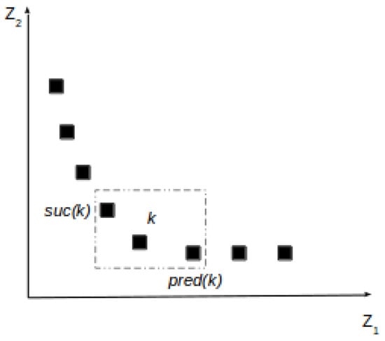
Figure 1.
Crowding distance.
The population update is illustrated in Figure 2 designed by Deb et al. [64]. Let t be the population rank. First, a population and the offspring population are merged to obtain a population of size . is then sorted out according to the non-domination criterion. Solutions in front are obviously of better quality and have to be conserved in the following population. However, if the size of the front is bigger than , only a part of the front is kept. In the case where the size of is strictly less than , the population has to be completed with solutions from the following fronts. In both cases, the choice is based on the crowding distance measure taken in descending order.
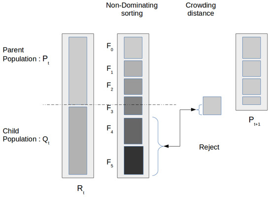
Figure 2.
Population update.
Basically, at each generation of NSGAII, an initial population () of individuals is generated and sorted according to the non-domination criterion. At each iteration, a child-population () containing individuals is produced. To get this population (), pairs of parents , are selected using the binary tournament method. Then, a crossover operator is applied to the two selected parents to obtain children, which are added to (). Finally, and are merged to obtain a mixed-population of size (). The latter is then sorted out (according to the non-domination criterion), and just the first solutions are retained to the next iteration. This process is repeated until a stopping condition is satisfied.
3.3. Encoding of A Solution
For VRPTW-SP, each solution is encoded as a vector of routes () in which each route is a sequence of customers that appear in the order they are visited by the associated vehicle, where delimiters are used to identify the routes. For example, Table 6 encodes a solution with three routes (vehicles) . The first is composed of Customer 1 followed by Customer 3, and the second route is composed of Customer 4, followed by Customer 7, which is followed by Customer 2, while the third route is composed of Customer 6 followed by Customer 5 (0 corresponds to the delimiter). Since our problem handles a fixed fleet size K, any vector has a size equal to (if all vehicles are used).
Table 6.
Encoding chromosome.
3.4. Initial Population
The generation of the initial population was done thanks to an adaptation of the Parallel Randomized constructive Heuristic (PRH), proposed to solve the VRPTW-SP in a previous work (see Ait Haddadene et al. [1]). Globally, this method uses a parallel strategy to generate solutions. A solution is created as follows: First, a route is opened for each available vehicle. Then, routes are fulfilled in a parallel way with customers selected from a sorted list of candidates ().
3.4.1. Construction of the Candidate List
Let i be the last customer visited by a vehicle (tour) k that offers the service s (at the beginning, i is the initial depot ). At each iteration, the following indicators are calculated for each unvisited customer j: the earliest time at which the vehicle k leaving i may be at the client j and the latest time when the vehicle leaving customer i can be at the customer j. and are respectively a lower and upper bound that ensure the return to the final depot in its time window. Then, the best client (elite) according to the minimum value of is selected among the list of candidates built as follows: a customer j is a candidate for a tour k under construction, if he/she has not yet been visited and if he/she satisfies the following conditions: , , and .
Here, a randomized version of the constructive heuristic is necessary to provide independent initial solutions (chromosomes). Randomness is based on the constructed list of candidates that is truncated to keep only the first clients. Then, the elite client is randomly chosen from this restricted list. The heuristic stops when all customers are inserted or when no more customers can be added to a vehicle (due to time window constraints and/or synchronization constraints).
It may result in a solution with unsatisfied customers. Thus, a second step considers all unvisited customers and tries to insert them at the first possible position in any existing route. These customers are taken in the increasing order of their starting availability time. However, if the solution is still not feasible, a new trial occurs on another close solution. This close solution is obtained by sequentially removing and inserting at another position (if possible) a fixed number of customers. This last process is repeated until reaching a feasible solution.
3.4.2. Improvement of the Initial Population
In order to improve the quality of these initial solutions, a Randomized Local Search () for the single objective VRPTW-SP is applied to each solution from . Its general structure is sketched in Algorithm 1. Here, the Pareto-dominance concept is not yet considered. At this point, the optimized objective function is . The considered moves are detailed in Section 3.6. Those are explored iteratively in a random sequence provided by a list of a certain size ( is the number of considered neighborhoods). In Line 5 of Algorithm 1, a neighborhood denoted by is chosen to be entirely explored. For example, we assume that Line 2 in Algorithm 1 gives the following sequence: {2, 3, 1}, then means that Neighborhood 2 is explored first until no more improvement is found, then Neighborhood 3 is selected, etc. In this case, .
| Algorithm 1 Randomized local search. |
|
3.5. Evolutionary Process
Two evolutionary processes are used to make a population evolve. The first one is a crossover operator employed once within a Non Dominated Sorting Genetic Algorithm (NSGAII) and then generalized to a new version called Multi-Start (MS-NSGAII). The second process consists of replacing the crossover and local search components by an iterated local search procedure.
3.5.1. Selection and Crossover Operators
The ordered crossover () is applied. At each iteration, a new population is generated by the process that selects two parent solutions and and generates children by applying the crossover operator. The selection is done following the binary tournament. For that, two solutions chosen randomly are compared. Then, the solution with the smallest rank is kept as . The same process is repeated to select . If two solutions belong to the same front, the crowded comparison prefers the one with the highest crowding distance.
Two child-solutions are then created by crossing the two selected parents using the ordered crossover () applied on each route. This is done as follows: a randomized crossover point is selected for each tour, then the two solutions are combined tour by tour to obtain two children. Figure 3 illustrates an example of the crossover operator. Crossing parents tour by tour allows us to meet the constraint related to vehicle skills (i.e., a client is visited by a vehicle offering its requested service). Nevertheless, the resulting child may be unfeasible in terms of customers/depot time windows, synchronization constraints, etc. Therefore, a repair procedure is called, and it is performed in three steps:
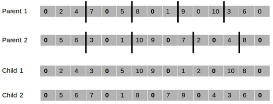
Figure 3.
Ordered crossover operator.
- Removing duplicates: If some customer appears in different routes, one of the different copies is randomly retained.
- Updating time visits: Time windows and synchronization constraint violation is prohibited. When a customer is not visited during his/her time window, he/she is removed from the solution. When a vehicle time window is violated, customers causing the violation are removed starting by the last customer of the corresponding route and coming up sequentially backward even for customers to be synchronized, provided that timing constraints are not respected or if the customers to be synchronized are inserted in contradictory positions (Figure 4 shows an example of a contradictory position of clients i and j to be eliminated). The corresponding customer is then deleted, and the vehicle arrival time to the final depot is updated.
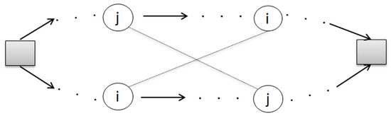 Figure 4. Contradictory positions of clients i and j.
 - Insertion of unsatisfied customers: All non-visited customers are considered and inserted in the first feasible position (the repair procedure explained at the end of Section 3.4 is used here).
Note that, in our previous paper Ait Haddadene et al. [1], feasibility tests implemented in constant time were proposed to check the feasibility of any insertion before its execution. These tests were applied here. In addition to the repair procedure, they were also used in the construction heuristic and in the local search.
Since the number of routes is related to the number of available vehicles (which is limited to ), the number of crossover points is equal to the number of used vehicles. In the case of an empty route (which means that the route is not opened for the corresponding vehicle), the child route will be a copy of the parent route.
3.5.2. Iterated Local Search Procedure
An iterated local search procedure is proposed to diversity and intensify the population. It consists of perturbing a solution with the aims to jump into another solution adjacent to the current one by introducing non-deterministic components (diversification). Then, a local search acts as the intensification. The problem of finding feasible solutions is difficult, because of timing constraints; that is why the perturbation mechanism performs a fixed number () of random exchange moves to introduce diversity while remaining within the set of feasible solutions. The resulting individual may be improved by applying a local search procedure (details are given in the next section). The process consisting of perturbing + improving is repeated times on the selected individual.
Technically, when a local search is applied on the perturbed solution, this leads to an iterated local search procedure. Remember that this method () initiates its search from a good quality solution. This means that a local search procedure is first applied on the current parent, with the aim of obtaining a first local optimum. Then, at each iteration of the , the current parent is perturbed with the intent to escape the local optima, which are generally grouped into clusters in the solution space. The resulting solution undergoes the local search to reach another local optimum. The incumbent solution is updated only in the case of improvement. The cycle consisting of perturbation and local search is repeated until the given number () of iterations is reached. The resulting solution is considered as a “child-solution”. This method allows us to maintain the feasibility of the solutions.
3.6. Local Search
This procedure may consist of generating neighborhoods using the first or best improvement strategy. In our study, preliminary tests have shown that looking for the best feasible move requires much time with limited gain in comparison with a first improvement strategy. That is why the latter has been selected. The whole local search stops when all neighborhoods are explored without finding any improvement.
Our neighborhoods are defined by simple commonly-used moves in VRP, involving one or usually more clients and/or one or more routes. They are the relocation and the two-exchange move, both executed on a single or different routes.
3.6.1. Acceptance Criteria for a Move
In the multi-objective context, a solution improves if it dominates it. In what follows, and respectively denote the total travel cost and the total non-preference value of a solution , and w is a real number belonging to .
The criteria tested to decide if converting a solution into is an improved one define two different strategies ( and ).
: the Pareto dominance: improves if .
However, it could be interesting to use an acceptance criteria based on the convex combination of the objective functions, such as done in . The main objective is to improve solutions in the first front conducting the search by descending values with emphasis on the extreme solutions, while preserving the space between solutions. These techniques were first introduced by [66]. For that, a pseudo-weight w must be computed for a given solution . In [66], the authors used Equation (5), in which and are respectively the minimum and the maximum values of criterion c ().
Then, an improving move is accepted if with .
3.6.2. Local Search Strategy
A classical way to add a local search in a genetic algorithm is to apply it on some of the child solutions. This is what was proposed in Strategy 1 with a call to on solutions of the child-population (Lines 6–8 of Algorithm 2). However, the Pareto-dominance is more strict than the acceptance criterion based on the convex combination of the objective functions. Thus, may be called post-optimization (Strategy 2) on solutions of the first front () obtained at the last population (Line 14 of Algorithm 2).
| Algorithm 2 Non-Dominated Sorting Genetic Algorithm (NSGAII). |
|
3.6.3. Local Search Frequency
For genetic algorithms (including the crossover operator), the local search procedure is called periodically. This means that the local search procedure is employed each generation. In this case, % solutions of the child-population undergo the local search, which are chosen according to the non-dominated sorting. For the NSILS (including the ILS procedure), the local search is applied systematically. This means that, at each generation, the local search is called, and in this case, % solutions of the child-population selected randomly undergo the local search. Table 7 summarizes all tested versions.
4. Pseudocodes
Now that all components have been defined, this section is devoted to the three pseudocodes tested in this article. The first is summarized in Algorithm 2 and is the general framework of NSGAII including the local search procedure.
To diversify the search, an idea is to restart NSGAII from another initial-population instead of loosing time in unproductive generations, thus giving what we call a Multi-Start Non-Dominated Sorting Genetic Algorithm (MS-NSGAII). Lines 1–15 of Algorithm 2 are repeated times. At the end of each restart, the best population is updated by mixing the last best population with the current-population of NSGAII. The latter is then sorted out (according to the non-domination criterion), and just the first solutions are retained. To test the same number of iterations as in Algorithm 2, an iteration of NSGAII inside MS-NSGAII consists of generations. The general structure of this approach is given by Algorithm 3.
| Algorithm 3 Multi-Start Non-Dominated Sorting Genetic Algorithm (MS-NSGAII). |
|
The third pseudocode is given in Algorithm 4. It is obtained by replacing the crossover operator of Algorithm 2 by the iterated local search procedure detailed in Section 3.5.2.
Other configurations were designed, especially for the percentage of involved solutions for the local search. However, only versions that appeared successful are shown in this paper. In total, seven versions were tested and compared on 37 instances.
| Algorithm 4 Non-Dominated Sorting Iterated Local Search Algorithm (NSILS). |
|
5. Computational Experiments
5.1. Implementation and Instances
Our algorithms were implemented in C language and executed on a 3.20-GHz Intel(R) Core(TM) i5-3470 CPU computer with 8 GB of RAM, running under Ubuntu. A set of HHC instances was designed by Bredström and Rönnqvist [17]. These instances include most of the particular features of the VRPTW-SP studied here: time windows, synchronization, and preferences. They were specifically extended to fit the additional problem specifications related to the different types of services offered to and requested by customers. The benchmark was grouped into three different categories according to the number of customers and vehicles, which were equal to 18 clients with 4 vehicles in the first group (), 45 clients with 10 vehicles in the second group (), and 73 clients with 16 vehicles in the third one (). In each group, the number of synchronizations ranged from 2-5, and the time windows could be small, medium, or large. In the extended version of instances, the customer demands and caregiver qualifications were randomly generated, but the rest of the information remained the same as in [17]. Without loss of generality, we only treated the case when at most two services were needed. The extended benchmark can be obtained by a simple request to the authors.
The file names followed an n-m-t-nb format, with clients, vehicles, referring to the width of the customer time windows (small, medium, or large,) and the last index corresponding to the maximum number of clients to be synchronized. These values were inspired from literature instances, where the number of synchronized customers did not exceed 10% of the total number of customers. All randomized algorithms were executed five times on each instance.
5.2. Evaluation Criteria
In this paper, the performance of the different versions of the algorithms was measured through five metrics:
- : The number of solutions in the first front .
- : The spacing measure proposed by Schott [67], which estimates the relative distance between two consecutive solutions obtained in the non-dominated set, as follows:where is the minimum value of the sum of the absolute difference in the objective function values between the solution and any other solution in the obtained non-dominated set. is the mean value of the above distance measure. When solutions are near uniformly spaced, the corresponding distance measure will be small. Thus, the method with smaller spacing is better.
- : The hyper-volume introduced by Zitzler et al. [68], which calculates the volume covered by members of . Mathematically, for each solution , a hyper-rectangle is constructed with a reference point. The reference point is defined by the maximal value of and obtained by all tested versions. Thereafter, a union of all hyper-rectangle is found, and the hyper-volume is calculated (see Figure 5). In this case, one method with a large value of is desirable.The spacing and the hyper-volume were not free from arbitrary scaling objectives, and then, the above metrics were evaluated by using normalized objective functions in the interval [0, 1]. For the hyper-volume measure, the selected reference point corresponded to the worst solution provided by all the tested versions.
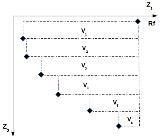 Figure 5. Hyper-volume for and of the Vehicle Routing Problem with Time Windows, Synchronization, and Precedence constraints (VRPTW-SP).
 - : The deviation from the optimal solution found by Cplex, which was used to solve the single-objective model in Ait Haddadene et al. [34], where was minimized. First, the best solution (called p) is identified by calculating the Euclidean distance of each solution in the first front to the optimal solution (called q). p corresponds to the solution with the smallest sum of the Euclidean distance. Then, the percentage of the deviation is calculated as follows:
- : The computational execution time reported in seconds.
5.3. Test Protocol and Parameters
For the set of instances, calibration with different configurations of parameters was used to see which version produced the best results. The best values that allowed obtaining a good compromise between solution quality and running time according to the performance measures mentioned above are shown in Table 8.
Table 8.
Fixed parameters. PRH, Parallel Randomized constructive Heuristic.
5.4. Numerical Results
Average results for the 37 test instances are shown for the different versions in Table 9, respectively for NSGAII, MS-NSGAII, and NSILS. In this table, the minimum (min), maximum (max), and the average values (av.) for the number of solutions in the first front (), the hyper-volume metric (), the spacing measure (), the percentage of the deviation from the optimal solution, and the time reported in seconds are given. As can been seen in Table 9, all versions with the local search procedure were better than versions without it, at a cost of a computing time about three-times higher on average.
Table 9.
Average results for the 7 versions on 37 instances. av., average.
In terms of the indicator, globally, NSGAII-1 found more solutions in the non-dominated Pareto front, offering the decision maker a set of solutions with a good compromise between the total travel cost and the customer preferences. Regarding the metric, all versions of the NSGAII and NSILS-2 methods were almost equivalent with a good coverage in the objective space by members from the non-dominated fronts.
According to the metric, from NSILS, applying was better. However, MS-NSGAII was practically equivalent to NSGAII for both local search-based methods. Furthermore, NSGAII-1 was the worst one according to this performance indicator. It is important to mention that the position of the solutions in the search space did not have a direct impact on the metric. Even when the metrics and were better, this did not guarantee better values for the metric.
According to the optimal deviation from optimal solutions and indicator, all versions found the optimal solution for and/or better with a good solution quality of . This shows that the methods were more accurate for than for . However, in general, NSILS can find better solutions than genetic methods according to , which is related to the minimization of the total travel cost. Therefore, it can be deduced that, even when the genetic aspect was not considered, but the non-dominated sorting was retained, the method obtained solutions of good quality, in a reasonable execution time. Once again, this metric allowed us to deduce the impact of the local search procedure in terms of convergence.
As can be expected, the running time () depended on the methods used. Those can be classified as follows: NSILS was more rapid than NSGAII, which was faster than MS-NSGAII. In accordance with the different variations of the proposed methods, NSGAII-1 and MS-NSGAII-1 required less computational time due to the way the local search was integrated. Note also that the mutation procedure was not used here, since preliminary tests showed that the crossover followed by local search led to better performance of the solution; thus, the mutation procedure was replaced by the latter.
5.5. Graphical Examples
Graphical representations are well suited to visualize the behavior of bi-objective optimization methods.
The two figures illustrate the impact of the local search procedure on the same instance. This is by comparing the efficient set computed by the basic version NSGAII-1 and MS-NSGAII-1 (no local search) with the other versions obtained local search strategies for each algorithm.
Figure 6 shows that hybridization with local search was necessary to obtain efficient solutions. Here for example, NSGAII-2 decreased the best travel cost of NSGAII-1 by approximately 73% (from ∼320 to ∼265) and the best non-preference by 5% (from ∼−200 to ∼−210). Thus, NSILS decreased the best travel cost of NSGAII−2 by approximately 5% (from ∼ 265 to ∼ 250). Moreover, several efficient solutions were obtained, and they were better spread, thus providing the decision maker with a wider choice.
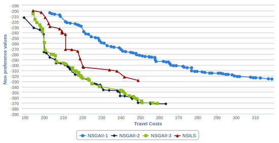
Figure 6.
Impact of local search for Instance 25 on NSGAII.
For the same instance, Figure 7 shows that all local search-based algorithms had a good convergence. However, NSGILS confirmed the numerical results, obtaining smaller fronts.
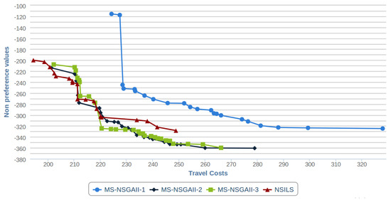
Figure 7.
Impact of local search for Instance 25 on MS-NSGAII.
Thus, from Figure 7, it is clear that MS-NSGAII-1 had not entirely converged and that MS-NSGAII-2 and MS-NSGAII-3 were more efficient, hence the interest in including local search procedures.
6. Conclusions
In this paper, population methods based on the NSGAII template with different local search strategies were presented in order to solve a bi-objective variant of the vehicle routing problem with time windows, in which both synchronization and precedence constraints were considered. The goal in this problem was to minimize the travel cost () while minimizing the customer non-preference (). This study was motivated by applications raised in home healthcare structures. A quick overview of vehicle routing problems with time windows and synchronization constraints was given. Special attention was accorded to existing works related to the home healthcare field, particularly those considering several optimization criteria.
Different local search-based versions of NSGAII were compared as well to the basic version of NSGAII. The effect of replacing the crossover operator and the local search procedure by an method was also evaluated. A new variant of NSGAII called MS-NSGAII was tested, where independent parent-populations were produced.
Computational experiments were carried out on 37 instances, which were extended from the benchmark initially proposed by Bredström and Rönnqvist [17]. To evaluate the performance of the developed algorithms, different measures that compared the obtained fronts were used. Additionally, the best and values were compared with the optimal solutions found by Cplex, which was used to solve the single-objective MILP in Ait Haddadene et al. [1]. After analyzing the different measures, the good performance of the proposed NSGAII version for solving the VRPTW-SP was established. The benefit of the local search procedure was clearly demonstrated, and results showed that including the local search procedure improved the solutions for both objectives, while the computational times were still reasonable. Finally, the proposed methods efficiently solved the VRPTW-SP and provided a large set of solution choices to the decision maker. As future work, other objective functions and local search moves may be considered. Moreover, the optimal Pareto front could be designed for more specific comparison.
Author Contributions
Conceptualization, N.L. and C.P.; Formal analysis, S.R.A.H., N.L. and C.P.; Investigation, S.R.A.H.; Software, S.R.A.H.; Supervision, N.L. and C.P.; Writing—original draft, S.R.A.H.; Writing—review & editing, N.L. and C.P.
Funding
This research received no external funding.
Conflicts of Interest
The authors declare no conflict of interest.
References
- Ait Haddadene, S.; Labadie, N.; Prodhon, C. A GRASP × ILS for the vehicle routing problem with time windows, synchronization and precedence constraints. Expert Syst. Appl. 2016, 6, 274–294. [Google Scholar] [CrossRef]
- Dantzig, G.; Ramser, J. The truck dispatching problem. Manag. Sci. 1959, 6, 80–91. [Google Scholar] [CrossRef]
- Toth, P.; Vigo, D. Vehicle Routing: Problems, Methods, and Applications; SIAM: Philadelpia, PA, USA, 2014. [Google Scholar]
- Vidal, T. General solution approaches for multi-attribute vehicle routing and scheduling problems. 4OR 2014, 12, 97–98. [Google Scholar] [CrossRef]
- Kindervater, G.; Savelsbergh, M. Vehicle routing: Handling edge exchanges. In Local Search in Combinatorial Optimization; Aarts, E., Lenstra, J., Eds.; Wiley: Chichester, UK, 1997; pp. 337–360. [Google Scholar]
- Bräysy, O.; Gendreau, M. Vehicle routing problem with time windows, part I: Route construction and local search algorithms. Transp. Sci. 2005, 39, 119–139. [Google Scholar] [CrossRef]
- Nagata, Y. Efficient Evolutionary Algorithm for the Vehicle Routing Problem with Time Windows: Edge Assembly Crossover for the VRPTW. In Proceedings of the 2007 IEEE Congress on Evolutionary Computation, Singapore, 25–28 September 2007; pp. 1175–1182. [Google Scholar]
- Bräysy, O.; Gendreau, M.; Tarantilis, C. Solving Large-Scale Vehicle Routing Problems with Time Windows: The State-of-the-Art; Technical Report; Montreal: Cirrelt, QC, Canada, 2010. [Google Scholar]
- Bodin, L.; Sexton, T. The multi-vehicle subscriber dial-a-ride problem. TIMS Stud. Manag. Sci. 1986, 2, 73–86. [Google Scholar]
- Cheng, E.; Rich, J. A Home Health Care Routing and Scheduling Problem; Technical Report CAAM TR98-04; Rice University: Houston, TX, USA, 1998. [Google Scholar]
- Fikar, C.; Hirsch, P. Home healthcare routing and scheduling: A review. Comput. Oper. Res. 2017, 77, 86–95. [Google Scholar] [CrossRef]
- Cissé, M.; Yalçındağ, S.; Kergosien, Y.; Şahin, E.; Lenté, C.; Matta, A. OR problems related to Home Health Care: A review of relevant routing and scheduling problems. Oper. Res. Health Care 2017, 13, 1–22. [Google Scholar] [CrossRef]
- Begur, S.; Miller, D.; Weaver, J. An integrated spatial DSS for scheduling and routing home-health-care nurses. Interfaces 1997, 27, 35–48. [Google Scholar] [CrossRef]
- Bertels, S.; Fahle, T. A hybrid setup for a hybrid scenario: Combining heuristics for the home healthcare problem. Comput. Oper. Res. 2006, 33, 2866–2890. [Google Scholar] [CrossRef]
- Eveborn, P.; Flisberg, P.; Rönnqvist, M. Laps Care—An operational system for staff planning of home care. Eur. J. Oper. Res. 2006, 171, 962–976. [Google Scholar] [CrossRef]
- Akjiratikarl, C.; Yenradee, P.; Drake, P. PSO-based algorithm for home care worker scheduling in the UK. Comput. Ind. Eng. 2007, 53, 559–583. [Google Scholar] [CrossRef]
- Bredström, D.; Rönnqvist, M. Combined vehicle routing and scheduling with temporal precedence and synchronization constraints. Eur. J. Oper. Res. 2008, 191, 19–31. [Google Scholar] [CrossRef]
- Steeg, J.; Schröder, M. A hybrid approach to solve the periodic home healthcare problem. In Operations Research Proceedings 2007; Springer: Berlin/Heidelberg, Germany, 2008; pp. 297–302. [Google Scholar]
- Hertz, A.; Lahrichi, N. A patient assignment algorithm for home care services. J. Oper. Res. Soc. 2009, 60, 481–495. [Google Scholar] [CrossRef]
- Redjem, R.; Kharraja, S.; Marcon, E. Collaborative model for planning and scheduling caregivers’ activities in homecare. IFAC World Congr. 2011, 44, 2877–2882. [Google Scholar]
- Trautsamwieser, A.; Gronalt, M.; Hirsch, P. Securing home healthcare in times of natural disasters. OR Spectr. 2011, 33, 787–813. [Google Scholar] [CrossRef]
- Trautsamwieser, A.; Hirsch, P. Optimization of daily scheduling for home healthcare services. J. Appl. Oper. Res. 2011, 3, 124–136. [Google Scholar]
- Nickel, S.; Schröder, M.; Steeg, J. Mid-term and short-term planning support for home healthcare services. Eur. J. Oper. Res. 2012, 219, 574–587. [Google Scholar] [CrossRef]
- Gamst, M.; Jensen, T. A branch-and-price algorithm for the long-term home care scheduling problem. In Operations Research Proceedings 2011; Springer: Berlin/Heidelberg, Germany, 2012; pp. 483–488. [Google Scholar]
- Rasmussen, M.; Justesen, T.; Dohn, A.; Larsen, J. The home care crew scheduling problem: Preference-based visit clustering and temporal dependencies. Eur. J. Oper. Res. 2012, 219, 598–610. [Google Scholar] [CrossRef]
- Redjem, R.; Kharraja, S.; Xie, X.; Marcon, E. Routing and scheduling of caregivers in home healthcare with synchronized visits. In Proceedings of the 9th International Conference on Modeling, Optimization & SIMulation, Bordeaux, France, June 2012. [Google Scholar]
- Afifi, S.; Dang, D.; Moukrim, A. A simulated annealing algorithm for the vehicle routing problem with time windows and synchronization constraints. In Learning and Intelligent Optimization; Springer: Berlin/Heidelberg, Germany, 2013; pp. 259–265. [Google Scholar]
- Liu, R.; Xie, X.; Augusto, V.; Rodriguez, C. Heuristic algorithms for a vehicle routing problem with simultaneous delivery and pickup and time windows in home healthcare. Eur. J. Oper. Res. 2013, 230, 475–486. [Google Scholar] [CrossRef]
- Hiermann, G.; Prandtstetter, M.; Rendl, A.; Puchinger, J.; Raidl, G. Metaheuristics for solving a multimodal home-healthcare scheduling problem. Cent. Eur. J. Oper. Res. 2013, 23, 89–113. [Google Scholar] [CrossRef]
- Allaoua, H.; Borne, S.; Létocart, L.; Wolfler-Calvo, R. A matheuristic approach for solving a home healthcare problem. Electron. Notes Discret. Math. 2013, 41, 471–478. [Google Scholar] [CrossRef]
- Liu, R.; Xie, X.; Garaix, T. Hybridization of tabu search with feasible and infeasible local searches for periodic home healthcare logistics. Omega 2014, 47, 17–32. [Google Scholar] [CrossRef]
- Labadie, N.; Prins, C.; Yang, Y. Iterated local search for a vehicle routing problem with synchronization constraints. In Proceedings of the ICORES 2014 3rd International Conference on Operations Research and Enterprise Systems, Angers, Loire Valley, France, 6–8 March 2014; pp. 257–263. [Google Scholar]
- Ait Haddadene, S.; Labadie, N.; Prodhon, C. GRASP for the Vehicle Routing Problem With Time Windows, Synchronization and Precedence Constraints. In Proceedings of the IEEE 10th International Conference on Wireless and Mobile Computing, Networking and Communications (WiMob), Larnaca, Cyprus, 8–10 October 2014; pp. 72–76. [Google Scholar]
- Ait Haddadene, S.; Labadie, N.; Prodhon, C. The VRP with Time Windows, Synchronization and Precedence Constraints: Application in Home Health Care Sector. In Proceedings of the MOSIM 2014, 10ème Conférence Francophone de Modélisation, Optimisation et Simulation, Nancy, France, 5–7 November 2014. [Google Scholar]
- Issaoui, B.; Zidi, I.; Marcon, E.; Ghedira, K. New Multi-Objective Approach for the Home Care Service Problem Based on Scheduling Algorithms and Variable Neighborhood Descent. Electron. Notes Discret. Math. 2015, 47, 181–188. [Google Scholar] [CrossRef]
- En-nahli, L.; Allaoui, H.; Nouaouri, I. A Multi-objective Modelling to Human Resource Assignment and Routing Problem for Home Health Care Services. IFAC-PapersOnLine 2015, 48, 698–703. [Google Scholar] [CrossRef]
- Maya Duque, P.; Castro, M.; Sörensen, K.; Goos, P. Home care service planning. The case of Landelijke Thuiszorg. Eur. J. Oper. Res. 2015, 243, 292–301. [Google Scholar] [CrossRef]
- Braekers, K.; Hartl, R.; Parragh, S.; Tricoire, F. A bi-objective home care scheduling problem: Analyzing the trade-off between costs and client inconvenience. Eur. J. Oper. Res. 2016, 248, 428–443. [Google Scholar] [CrossRef]
- Afifi, S.; Dang, D.; Moukrim, A. Heuristic solutions for the vehicle routing problem with time windows and synchronized visits. Optim. Lett. 2016, 10, 511–525. [Google Scholar] [CrossRef]
- Fikar, C.; Hirsch, P. Evaluation of trip and car sharing concepts for home healthcare services. Flex. Serv. Manuf. J. 2016, 30, 78–97. [Google Scholar] [CrossRef]
- Heching, A.; Hooker, J. Scheduling home hospice care with logic-based benders decomposition. Lect. Notes Comput. Sci. 2016, 9676, 187–197. [Google Scholar]
- Lin, M.; Chin, K.; Wang, X.; Tsui, K. The therapist assignment problem in home healthcare structures. Expert Syst. Appl. 2016, 62, 44–62. [Google Scholar] [CrossRef]
- Redjem, R.; Marcon, E. Operations management in the home care services: A heuristic for the caregivers’ routing problem. Flex. Serv. Manuf. J. 2016, 28, 280–303. [Google Scholar] [CrossRef]
- Shi, Y.; Boudouh, T.; Grunder, O. A hybrid genetic algorithm for a home healthcare routing problem with time window and fuzzy demand. Expert Syst. Appl. 2017, 72, 160–176. [Google Scholar] [CrossRef]
- Wirnitzer, J.; Heckmann, I.; Meyer, A.; Nickel, S. Patient-based nurse rostering in home care. Oper. Res. Health Care 2016, 8, 91–102. [Google Scholar] [CrossRef]
- Yalçındag, S.; Matta, A.; Sahin, E.; Shanthikumar, J.G. The patient assignment problem in home healthcare: Using a data-driven method to estimate the travel times of care givers. Flex. Serv. Manuf. J. 2016, 28, 304–335. [Google Scholar] [CrossRef]
- Decerle, J.; Grunder, O.; El Hassani, A.H.; Barakat, O. A general model for the home healthcare routing and scheduling problem with route balancing. IFAC-PapersOnLine 2017, 50, 14662–14667. [Google Scholar] [CrossRef]
- Du, G.; Liang, X.; Sun, C. Scheduling optimization of home healthcare service considering patients’ priorities and time windows. Sustainability 2017, 9, 253. [Google Scholar] [CrossRef]
- Frifita, S.; Masmoudi, M.; Euchi, J. General variable neighborhood search for home healthcare routing and scheduling problem with time windows and synchronized visits. Electron. Notes Discret. Math. 2017, 58, 63–70. [Google Scholar] [CrossRef]
- Laesanklang, W.; Landa-Silva, D. Decomposition techniques with mixed integer programming and heuristics for home healthcare planning. Ann. Oper. Res. 2017, 256, 93–127. [Google Scholar] [CrossRef]
- Decerle, J.; Grunder, O.; El Hassani, A.H.; Barakat, O. A memetic algorithm for a home healthcare routing and scheduling problem. Oper. Res. Health Care 2018, 16, 59–71. [Google Scholar] [CrossRef]
- Fathollahi-Fard, A.M.; Hajiaghaei-Keshteli, M.; Tavakkoli-Moghaddam, R. A bi-objective green home healthcare routing problem. J. Clean. Prod. 2018, 200, 423–443. [Google Scholar] [CrossRef]
- Lin, C.C.; Hung, L.P.; Liu, W.Y.; Tsai, M.C. Jointly rostering, routing, and rerostering for home healthcare services: A harmony search approach with genetic, saturation, inheritance, and immigrant schemes. Comput. Ind. Eng. 2018, 115, 151–166. [Google Scholar] [CrossRef]
- Nasir, J.; Dang, C. Solving a more flexible home healthcare scheduling and routing problem with joint patient and nursing staff selection. Sustainability 2018, 10, 148. [Google Scholar] [CrossRef]
- Liu, R.; Tao, Y.; Xie, X. An adaptive large neighborhood search heuristic for the vehicle routing problem with time windows and synchronized visits. Comput. Oper. Res. 2019, 101, 250–262. [Google Scholar] [CrossRef]
- Moussavi, S.; Mahdjoub, M.; Grunder, O. A matheuristic approach to the integration of worker assignment and vehicle routing problems: Application to home healthcare scheduling. Expert Syst. Appl. 2019, 125, 317–332. [Google Scholar] [CrossRef]
- Liu, R.; Yuan, B.; Jiang, Z. Mathematical model and exact algorithm for the home care worker scheduling and routing problem with lunch break requirements. Int. J. Prod. Res. 2017, 55, 558–575. [Google Scholar] [CrossRef]
- Drexl, M. Synchronization in vehicle routing-A survey of VRPs with multiple synchronization constraints. Transp. Sci. 2012, 46, 297–316. [Google Scholar] [CrossRef]
- Jozefowiez, N.; Semet, F.; Talbi, E. Enhancements of NSGAII and Its Application to the Vehicle Routing Problem with Route Balancing; Artificial Evolution; Springer: Berlin/Heidelberg, Germany, 2006; pp. 131–142. [Google Scholar]
- Lacomme, P.; Prins, C.; Sevaux, M. A genetic algorithm for a bi-objective capacitated arc routing problem. Comput. Oper. Res. 2006, 33, 3473–3493. [Google Scholar] [CrossRef]
- Velasco, N.; Dejax, P.; Guéret, C.; Prins, C. A non-dominated sorting genetic algorithm for a bi-objective pick-up and delivery problem. Eng. Optim. 2012, 44, 305–325. [Google Scholar] [CrossRef]
- Issabakhsh, M.; Hosseini-Motlagh, S.M.; Pishvaee, M.S.; Saghafi Nia, M. A vehicle routing problem for modeling home healthcare: A case study. Int. J. Transp. Eng. 2018, 5, 211–228. [Google Scholar]
- Marcon, E.; Chaabane, S.; Sallez, Y.; Bonte, T.; Trentesaux, D. A multi-agent system based on reactive decision rules for solving the caregiver routing problem in home healthcare. Simul. Model. Pract. Theory 2017, 74, 134–151. [Google Scholar] [CrossRef]
- Deb, K.; Pratap, A.; Agarwal, S.; Meyarivan, T. A fast and elitist multiobjective genetic algorithm: NSGA-II. Evol. Comput. IEEE Trans. 2002, 6, 182–197. [Google Scholar] [CrossRef]
- Labadie, N.; Melechovsky, J.; Prins, C. An evolutionary algorithm with path relinking for a bi-objective multiple traveling salesman problem with profits. In Applications of Multi-Criteria and Game Theory Approaches; Springer: Berlin/Heidelberg, Germany, 2014; pp. 195–223. [Google Scholar]
- Murata, T.; Nozawa, H.; Ishibuchi, H.; Gen, M. Modification of Local Search Directions for Non-Dominated Solutions in Cellular Multiobjective Genetic Algorithms for Pattern Classification Problems; Evolutionary Multi-Criterion Optimization; Springer: Berlin/Heidelberg, Germany, 2003; pp. 593–607. [Google Scholar]
- Schott, J. Fault Tolerant Design Using Single and Multicriteria Genetic Algorithm Optimization. Master’s Thesis, Massachusetts Institute of Technology, Dept. of Aeronautics and Astronautics, Cambridge, MA, USA, 1995. [Google Scholar]
- Zitzler, E.; Thiele, L.; Laumanns, M.; Fonseca, C.; Da Fonseca, V. Performance assessment of multiobjective optimizers: An analysis and review. IEEE Trans. Evol. Comput. 2003, 7, 117–132. [Google Scholar] [CrossRef]


© 2019 by the authors. Licensee MDPI, Basel, Switzerland. This article is an open access article distributed under the terms and conditions of the Creative Commons Attribution (CC BY) license (http://creativecommons.org/licenses/by/4.0/).