Article

Triplet Loss Network for Unsupervised Domain Adaptation

by
Imad Eddine Ibrahim Bekkouch
1,*,
Youssef Youssry
1,
Rustam Gafarov
1,
Adil Khan
1 and
Asad Masood Khattak
2
1
Machine Learning and Knowledge Representation Lab in the Institute of Data Science & AI, Innopolis University, Innopolis 420500, Republic of Tatarstan, Russia
2
College of Technological Innovations, Zayed University, Abu Dhabi 144534, United Arab Emirates
*
Author to whom correspondence should be addressed.
Algorithms 2019, 12(5), 96; https://doi.org/10.3390/a12050096
Submission received: 25 March 2019 / Revised: 30 April 2019 / Accepted: 2 May 2019 / Published: 8 May 2019
(This article belongs to the Special Issue Deep Learning for Image and Video Understanding)

Abstract

:
Domain adaptation is a sub-field of transfer learning that aims at bridging the dissimilarity gap between different domains by transferring and re-using the knowledge obtained in the source domain to the target domain. Many methods have been proposed to resolve this problem, using techniques such as generative adversarial networks (GAN), but the complexity of such methods makes it hard to use them in different problems, as fine-tuning such networks is usually a time-consuming task. In this paper, we propose a method for unsupervised domain adaptation that is both simple and effective. Our model (referred to as TripNet) harnesses the idea of a discriminator and Linear Discriminant Analysis (LDA) to push the encoder to generate domain-invariant features that are category-informative. At the same time, pseudo-labelling is used for the target data to train the classifier and to bring the same classes from both domains together. We evaluate TripNet against several existing, state-of-the-art methods on three image classification tasks: Digit classification (MNIST, SVHN, and USPC datasets), object recognition (Office31 dataset), and traffic sign recognition (GTSRB and Synthetic Signs datasets). Our experimental results demonstrate that (i) TripNet beats almost all existing methods (having a similar simple model like it) on all of these tasks; and (ii) for models that are significantly more complex (or hard to train) than TripNet, it even beats their performance in some cases. Hence, the results confirm the effectiveness of using TripNet for unsupervised domain adaptation in image classification.

1. Introduction

Computer vision (CV) applications have recently witnessed a revolution, thanks to deep learning techniques which leverage hierarchical pattern learning techniques and vast amounts of data to solve several challenging tasks with high accuracy. Despite their high recognition performance, as a natural result of using a specific dataset, even the deep models are biased to the domain from which the data are collected; which causes the performance of these models to decrease dramatically when tested against datasets from different domains.
The primitive solution to this problem is to adapt the model to the new (or target) domain by re-training the model on the data from the target domain. However, the collection of new data and the re-training of the whole model can be difficult, expensive, and even impossible. Hence, a better approach is to store the knowledge learned in the primary domain and later transfer that knowledge to a target domain sharing the same tasks but potentially following a different distribution. This can help in reducing the cost of data re-collection and its labelling.
More formally, let D s and D t be the source and target domains, respectively. Domain adaptation (DA), which is a sub-field of transductive transfer learning (TTL), aims to solve a problem in D t , where data are hard to collect, using data from D s . Both domains, usually, share the same tasks (i.e., T t = T s ) but the marginal distributions of the inputs differ (i.e., P ( X s ) P ( X t ) ), as shown in Figure 1. DA is usually achieved by learning a shared feature space (i.e., Z s = Z t ) [1].
There is a sizeable literature on DA. It can be categorized as either closed-set [2] or open-set [3,4]. Closed-set DA is the case where the classes of D t are the same as that of D s . Our work belongs to closed-set DA. On the other hand, open-set DA handles the case where only a few classes are shared between the two domains, and the source or the target domain might contain more classes.
Similar to other machine learning tasks, DA can be split into supervised, unsupervised, and semi-supervised, depending on how much labeled data are available from D t . For supervised domain adaptation (SDA) [5] and semi-supervised domain adaptation (SSDA) [6], the data are completely or partially labeled, but are not sufficient enough to train an accurate model for the target domain from scratch. In unsupervised domain adaptation (UDA) [7,8] the target domain samples are completely unlabeled, which is useful in situations where the data collection process is easy but the data labeling process is time consuming.
The extreme case of DA is when we don’t have any access to the target data, which is called domain generalization (DG). In DG, researchers have mainly used easy-to-collect datasets from different domains to make a model that can generalize well to unseen domains [9].
The focus of this work is on UDA, which typically needs large amounts of target data, especially in the case of deep unsupervised domain adaptation (DUDA). Although the focus is on DUDA because of the wide variety of real-world applications that it can solve, we use SDA as an upper bound to aim for, because SDA typically outperforms UDA, and we will exploit this fact to make our model perform even better by using a concept called pseudo-labelling [10]. Most of the previous DUDA approaches aimed at achieving two targets: (i) Produce (or learn) feature vectors from the data from D s that can be used by a classifier to get highly accurate class labels, and (ii) make the features of both D s and D t indistinguishable. Both Z. Ren et al., in [11], and Lanqing Hu et al., in [12], used generative models in different manners to achieve those targets. The former used Generative Adversarial Networks (GAN) to reconstruct various property maps of the source images while keeping the features extracted of both domains similar by training a base encoder on the opposite loss of the discriminator. The latter work used a duplex GAN architecture that could reconstruct the input images in both flavours, source and target, using the features extracted from the encoder. Next, a duplex discriminator was trained to distinguish the reconstructed images into source and target.
Our model is motivated by the latter work, yet it is much simpler. More specifically, we show that the generative part is hard to train and is not necessary to obtain a domain adaptive model. By introducing novel loss functions, we show that our model produces comparable results to the state-of-the-art models in a computationally efficient way.
To conclude, in this work, we make the following contributions:
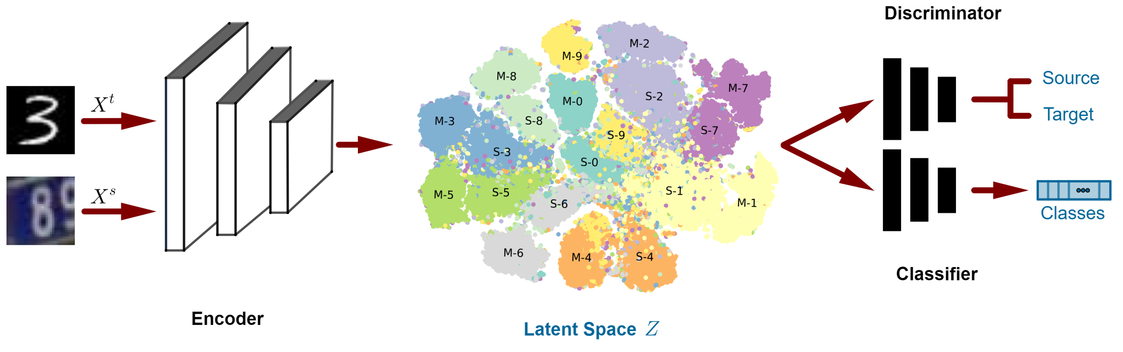
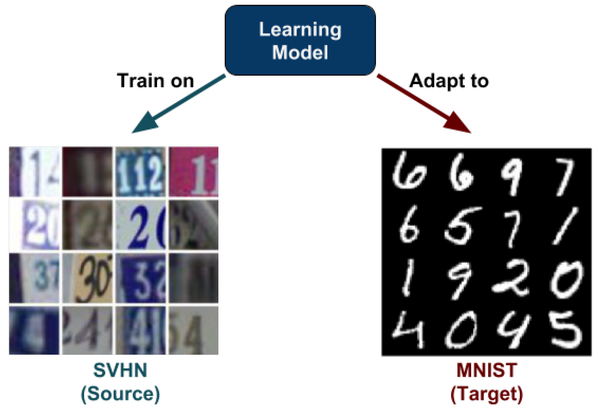
  • We implement a novel DUDA technique for image classification. Deep (D) because it consists of an auto-encoder, a discriminator, and a classifier—all of which are simple deep networks. Unsupervised (U) because we do not use the actual annotations of the target domain. Domain adaptation (DA) because, while learning the model using source data, we adapt it such that it performs well on the target domain, too.
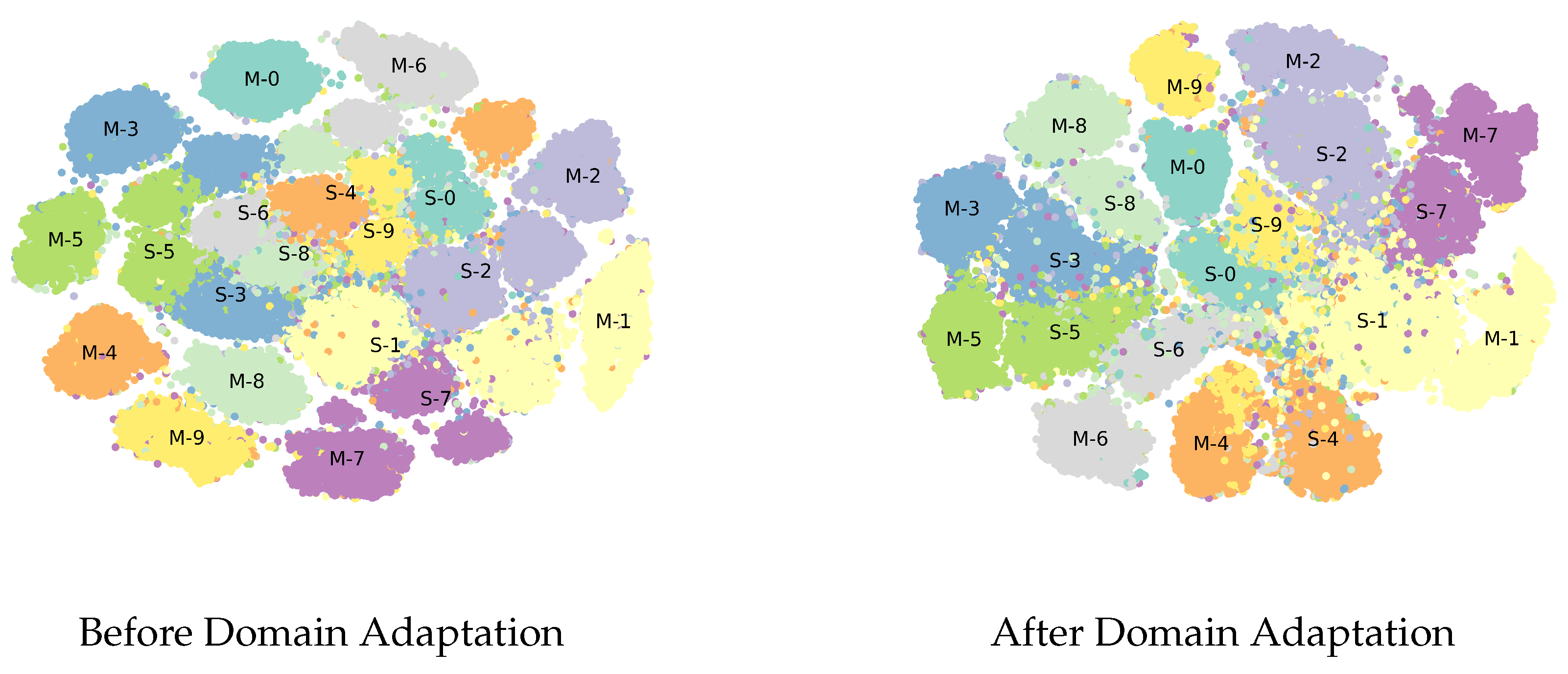
  • Our approach obtains a domain adaptive model by introducing separability loss, discrimination loss, and classification loss, which works by generating a latent representation that is both domain-invariant and class informative, by pushing samples from the same classes and different domains to share similar distributions.
  • We compare the performance of our model against several existing state-of-the-art works in DA on different image classification tasks.
  • Through extensive experimentation, we show that our model, despite its simplicity, either surpasses or achieves similar performance to that of the state-of-the-art in DA.
The rest of the sections are organized as follows: Section 2 provides a brief of the main contributions in DA. Section 3 presents our model architecture and our novel loss function. Details of our experimental setup, datasets, and empirical results are shown in Section 4. Finally, Section 5 wraps up the paper.

2. Related Work

In solving the problem of UDA, recent works used deep learning in various ways to build their models. A discriminator module was the core in most of the papers [11,12,13,14], and its loss was used to tell if the features extracted from both domains were distinguishable or not. Within the works that used the discrimination loss, several were based on generative models [11,12] and their reconstruction loss [15,16], and some used pseudo-labeling [10,12,17,18,19,20] to engage the target domain data into the process of classification. In this regard, our model is an example of the case where discrimination loss and pseudo-labeling are used without any reconstruction of the input images. We briefly touch upon these topics below.

2.1. Discriminator

The works [11,13,14] used the discriminator in the same manner. The discriminator was fed by the feature vectors of the source and target images and its loss was used to push the base/encoder/feature extractor network to produce indiscriminate features. In [12], the feature vectors were used to generate images in both source and target domains, and those images were fed into one of two discriminators that distinguished between real and fake images. This methodology was designed to ensure that the features extracted from the encoder network could be used to generate images of both domains; in other words, the features were domain-invariant.

2.2. Image Reconstruction

Similar to the image-to-image translation scenario, image reconstruction can be used in an Encoder–Decoder-like architecture to drive the encoder to generate features for both domains, so that the model can reconstruct the image regardless of its domain. For example, in [15,16] a bi-shifting auto-encoder (BAE) and an invertible AE used the reconstruction loss to convert samples between domains.

2.3. Generative Models

For the purpose of mitigating domain discrepancy, [12,21,22] tried to find a mapping between the two domains using cycle GANs [19,23], where DupGAN [12] achieved promising results in learning a domain-invariant latent representation. In their model, the generator was trained against two discriminators, one for each domain, resulting in one of the state-of-the-art performances in unsupervised domain adaptation. Similarly, [19,23] used the generator module to generate images from both domains using the same latent representation, which helped to verify that the encoder had lost domain-style information and had generated domain-invariant representations. Lv et al. [24] used a Coupled GAN to learn the joint distribution of multiple domains, in an unsupervised manner, through enforcing a weight-sharing constraint to the classifier network and, partially, to the GAN architecture. In [25], S. Sankaranarayanan et al., used a two-stream architecture: The first was a normal encoder-classifier network, and the other was an Auxiliary Classifier GAN (ACGAN) where the discriminator worked as a base for two classifiers: (1) For image labels, and (2) for image domains.

2.4. Pseudo-labeling

Pseudo-labeling is a commonly-used method in semi-supervised learning. In UDA, pseudo-labeling is used for narrowing the gap between the target and source domains, by providing pseudo-labels for the unlabeled samples from the target domain. In [19], two classifiers were used to label the unlabeled target data, which was used further in training the rest of the components. On the other hand, in [20], the researchers used a similarity metric in building a K-Nearest Neighbours (K-NN) graph for the unlabeled target samples and the labeled source samples. In DupGAN [12], a classifier, built on the labeled source images, was used to obtain high-confidence images from the target domain, which were then used to train both the classifier and the discriminators.

3. Architecture and Methodology

3.1. Overview

The following section describes the proposed model for UDA. We start by defining the notation that we use. The source domain images and labels are denoted as X s = ( x i s , y i s ) i = 1 N and the target domain images are X t = ( x i t ) i = 1 M ; both x i s and x i t share the same dimensions, but different distributions. As our research focuses on closed-set domain adaptation, the target and source domain labels Y are exactly the same.
Our model contains an encoder, a classifier, and a discriminator, as shown in Figure 2. The encoder and the classifier make up the final classification model, and the discriminator is used to train the encoder to generate domain-invariant features. Hence, our classification function f is the composition of two functions f = e c , where e : X Z is the encoding function that maps the images into feature vectors and c : Z Y categorizes the features for both domains. The discrimination function g is also the composition of two functions g = e d , where e is the same encoding function and d : Z A is the binary classification function that discriminates the domain of the latent representation of the input image.
In addition to the usual classification and discrimination loss, we introduced a separation loss that operates on the output of the encoder, similar to Linear Discriminant Analysis (LDA).

3.2. Architecture

Encoder: The encoder E ( . ) is a Convolutional Neural Network (CNN)-like network with weights W E . The target of the encoder is to produce the latent representation of both source and target domain images, as below:
z = E ( x ) , x X s X t ,
where z Z are the extracted features that we aim to be domain-invariant and category-informative. Therefore, in the case of an input image from the source domain x s , the output of the encoder is z s = E ( x s ) ; and if the image is from the target domain x t , then the output is z t = E ( x t ) . The output of the encoder is fed to both the discriminator and the classifier.
Discriminator: Discrimination between the source and the target in the latent space is a core part in many of the recent contributions in DA, as was mentioned in Section 2. Our Discriminator D ( . ) is a DNN with weights W D . The discriminator works as a binary classifier to label the latent representation of the images to one of the domains, as follows:
a = D ( z ) = D ( E ( x ) ) , a A , A = { 0 , 1 } .
Classifier: The classifier is a feed-forward neural network C ( . ) with weights W C for either binary or multi-class classification. It takes, as input, the latent representation z and outputs the probabilities for each class y ^ . C can be any kind of DNN with a softmax output activation function that fulfills the tasks T t and T s .
In the case of multi-class classification, C predicts the class probabilities, as follows:
y ^ = C ( z ) = C ( E ( x ) ) , x X , X = X s X t ,
where y ^ is the vector of predicted class probabilities for the images of both domains y ^ Y ^ , Y ^ = Y ^ s Y ^ t , and it shares the same dimensions as the one-hot-encoded source labels y s and the target pseudo-labels y t . The classifier C and the encoder E are pre-trained on the source data alone, and are then used to generate the pseudo-labels for the target domain Y t [12,26,27] , using the output of the classifier on the target images that C is highly confident about. In the beginning, the number of samples chosen for pseudo-labeling will be small, or even zero, but it increases as we get more domain-invariant features.

3.3. Losses

Here, we introduce our three losses and explain how each one contributes to achieve domain-invariant and category-informative features.
Classification Loss: This is the usual cross-entropy loss H ( , . , ) for the output of source images and their labels and the output of target images (chosen for pseudo-labeling) and their corresponding pseudo-labels, and is computed as follows:
L c ( W E , W C ) = λ s x s X s H ( y ^ s , y s ) + λ t x t X t H ( y ^ t , y t ) ,
where λ s and λ t are used to balance the weighted sum between the source and the target, since we only take a few samples using pseudo-labeling. By minimizing this loss, we update the weights of both the encoder and the classifier, W E and W C .
Discrimination Loss: In order to get domain-independent features, we used the discrimination loss to train the discriminator to distinguish between the features for both domains, using binary cross-entropy, as follows:
L D ( W D ) = z s Z s log ( D ( z s ) ) z t Z t log ( 1 D ( z t ) ) ,
which can be written as:
L D ( W D ) = x s X s log ( D ( E ( x s ) ) ) x t X t log ( 1 D ( E ( x t ) ) ) ,
where we assign 1 to the source images and 0 to the target images. The weights of the discriminator W D are updated by minimizing this loss as an objective function. The encoder is trained against an opposite loss that tries to put them in the same label, as follows:
L P ( W E ) = x s X s log ( 1 D ( E ( x s ) ) ) .
L P is used to update the encoder, such that the discriminator is deceived into thinking that the features extracted from both domains are indistinguishable. We also tried to deceive the discriminator using other loss variations, one aimed at pushing the domains in the exact opposite direction (i.e., target → 1 and source → 0) by adding x t X t log ( D ( E ( x t ) ) to L P , and another loss aimed at pushing both the source and the target into the same label by adding x t X t log ( 1 D ( E ( x t ) ) to L P in Equation (7), but these variations didn’t improve the results and caused the model to diverge with more iterations. L D and L P work against each other in a scenario similar to GAN discrimination loss and generative loss.
Separability Loss: Inspired by Linear Discriminant Analysis (LDA) to capture the separability, Ficher [28] defined an optimization function to maximize the between-class variability and minimize the within-class variability. Using this idea, we defined the separability loss, as follows:
L s e p ( W E ) = i Y z i j Z i d ( z i j , μ i ) i Y d ( μ i , μ ) × λ B F ,
λ B F = min i | Y i t | max i | Y i t | ,
where Z i is the set of latent variables that belongs to class i, which can be expressed as Z i = Z i s Z i t ; the union of the sets of latent representation of both domains that have the same label i. Again, for the target domain latent representation, we used the pseudo-labels that were produced with a high level of confidence from the classifier. Further, μ i is the mean of the latent representations that have label i, so it can be expressed as μ i = m e a n ( Z i ) , while μ is the mean of all the latent representations, μ = m e a n ( Z ) ; d ( . , . ) is a distance function we use to measure the dissimilarity between the latent vectors. So, the numerator part of the equation is the summation of the distance between each latent vector and its labeled-center, while the denominator is the summation of the distance from each labeled-center to the overall center of the latent representation; λ B F is a balancing factor and is equal to the ratio between the number of least-represented pseudo-labeled target samples min i | Y i t | and the number of the most-represented ones max i | Y i t | , where i is the label. The purpose of this is to pull the loss from converging to some local minima if some classes are not well-represented in the pseudo-labels. Thus, λ B F keeps the separability loss from pushing the model into a very high separability and accuracy in only a subset of the classes. Thus, by minimizing this loss function, we can increase the separability of the latent representation, according to the labels and regardless of domain, which drives the encoder to lose domain-specific features but preserve category-informative features. It should be noted that the generator component in DupGAN [12] has the same purpose: It uses the extracted features to generate images in both domains to ensure that they are domain-invariant, and reconstructs the input image to ensure that the features do not lose the category information. However, by using a loss function, instead of a separate generator module, this work achieves the said purpose in a cost-effective manner.

3.4. Optimization

The overall objective function that we aim to minimize in this work is the weighted sum of the three losses, which we call the triplet loss, and is given as follows:
L = min W D , W C , W E β C L C + β P L P + β S e p L S e p ,
where β C , β P , and β S e p are the balancing parameters. The detailed training process of our model, called TripNet, is described in Algorithm 1. The input number of iterations ranges from 500–1000.
Algorithm 1: The training process of TripNet
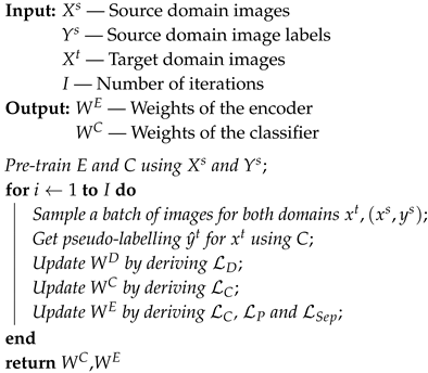
   Algorithms 12 00096 i001

3.5. Novelty

The main novelty of our work is imposing the separability loss on the latent representation of both domains, in order to drive the encoder to close the gap between the two domains by clustering the latent representations of images using their labels (regardless of their domain) and keeping the class information within this latent space. At the same time, we use pseudo-labeling for the target domain to compensate for the absence of labeled data in the target domain.

4. Experiments and Results

We compared our model with several state of the art models, including DupGAN [12], TarGan [24], Maximum Classifier Discrepancy (MCD) [29], Gen2Adpt [25], SimNet [13], Domain-Adversarial Training of Neural Networks (DANN) [30,31], T. Adversarial Discriminative Domain Adaptation (ADDA) [32], Domain Separation Networks (DSN) [33], Deep Reconstruction-Classification Networks (DRCN) [34], Coupled Generative Adversarial Networks (CoGAN) [35], Unsupervised Image-to-Image Translation Networks (UNIT) [36], RevGrad [30], PixelDA [37], kNN-Ad [20], Image2Image [21], and Asymmetric Tri-training for Unsupervised Domain Adaptation (ATDA) [27], for digit classification and object recognition. As we followed the same experimental set-up as the one that was employed for the compared networks, we evaluated our model based on the accuracy on the target test set, as this was the most-used metric within the previous works, which will enable us to compare it with the previously-mentioned papers using their reported results. The comparison will be made on three different tasks: (1) Digit classification, (2) object recognition, and (3) simulation-to-real object recognition. Then, we compare our model against DupGAN in terms of complexity (number of iterations).
We will also compare our model against itself, using just the encoder and the classifier trained on the source domain only (noted as training on source only) and the target domain only (noted as training on target labels) to give a lower bound and approximation of the upper bound. This comparison, shown in Table 4, shows the degradation of the accuracy of the target domain before domain adaptation in the EC-SourceOnly row. This demonstrates the effectiveness and the usefulness of the adaptation technique generally, and our model specifically.

4.1. Target Accuracy Comparison

4.1.1. Digit Classification

Our model was evaluated for UDA for the digit classification task, where the labels are 0 ∼ 9, using different datasets: MNIST of handwritten digits [38], SVHN of street houses numbers [39]; and the USPS [40] of U.S. Postal Service Handwritten Digit Database. These datasets were chosen because they have different distributions and their labels are present for validation and evaluation. We used 60,000 images from MNIST from its training part and 10,000 images from its evaluation part. USPS is a relatively smaller dataset, from which we used 7291 images for training and 2007 images for testing. Finally, SVHN had 73,257 images for training, 26,032 images for testing, and SVHNextra had 531,131 additional images for training. Our experiments were SVHN → MNIST, USPS ↔ MNIST, and SVHNextra→ MNIST.
The target accuracy results are shown in Table 1, where we can see first the decrease in performance when changing the domain (first two rows): For SVHN → MNIST, we see a decrease of 36.6%; on average, there was a 23% decrease across all experiments, proving the need for domain adaptation methods. Our novel model either exceeded the compared methods or approached the highest-achieved results. It is also noteworthy that our model was so close to the results of a model that was trained on the target only, and surpassed it in some cases. This is due to the use of the separation loss and the discriminator, which allowed our latent representations to be domain-invariant, as seen in Figure 3, where all classes were clustered together, regardless of domain.
Figure 3 illustrates the projection of the latent representations of both domains in the first experiment, SVHN → MNIST. The projection for the visualization was produced using T-SNE [41] by reducing the dimensions of the latent space from 512 into 2, for visualization purposes. In Figure 3, it can be noticed that, after domain adaptation, the clusters for both domains that carry the same labels settled close to each other in the latent space, which demonstrates the competence of the presented model.
According to the results presented in Table 1, there was no one specific model which outperformed the others in all cases. Those that exceeded our model (though, not by a significant margin) had more complex architectures and were difficult to train. We highlight this point later, in Section 4.2.

4.1.2. Object Recognition using OFFICE31

We also evaluated our method on the OFFICE dataset [42] for object recognition. Office31 is a widely-used dataset in domain adaptation, containing images belonging to 31 different classes gathered from three different domains: Amazon (A), Webcam (W), and DSLR (D). One of the major challenges in this dataset is that it contains only 4110 images (A:2817, W:795, and D: 498), which is too small to build any deep classifier. Most DUDA methods tend to use a pre-trained model (like AlexNet [43] or ResNet [44]) and fine-tune it to this specific dataset. In our method, we chose to use a pre-trained AlexNet and replaced the final layer with a dense (4096,31) fully-connected layer, instead of the dense (4096,1000) layer. We followed the same protocol as for the digit classification task. We report our results in Table 2. We can see that our model provided state-of-the-art performance on AlexNet-based models (rows above our model) and even beat the ResNet-based models on the D → W experiment, even though we used a much smaller network; as we aimed to design a simple model with good adaptation ability, ease to training, and, yet, which provides better performance as well. It is apparent, from our results, that indeed our model beat (or provided similar results to) most existing methods. It is also worth mentioning that the cited ResNet-based models did not show a significant increase in accuracy, ranging from 0.5% to a maximum of 11% of accuracy increase, when compared against the vanilla ResNet (last row in Table 2).

4.1.3. SYN-SIGNS to GTSRB

Our last comparison will be on the German traffic signs recognition benchmark (GTSRB) datasets and Synthetic Signs (SYN-SIGNS) dataset. The goal of this evaluation is to evaluate the use of DA in generalizing to real-world images using synthetic data. Both datasets were split into 43 different traffic signs. We used 10,000 labeled SYN-SIGNS images as the source domain, and 31,367 GTSRB images as training data; while 3000 GTSRB images were used for validation and the rest of the images were used as a test set for evaluating the final performance. We used the same experimental setup as the one in the digits experiment, with the same model and network architecture.
We can definitely see an improvement, from 56.4–88.7% (Table 3). Although our model was behind the state-of-the-art in this experiment, it is important to note that consumed less computational resources and converged much faster.

4.2. Comparison of TripNet and DupGAN

We conducted a comparison between the convergence of TripNet and DupGAN for the experiment SVHN → MNIST, as shown in Figure 4, within the same experimental setup. It is clear that our model converged significantly faster—after just the first 120 iterations—whereas DupGAN didn’t even approach its maximum accuracy after 500 iterations. Based on our experiments, we found that the generative model DupGAN needs roughly 100 times the number of iterations that TripNet needed to reach its maximum accuracy.

4.3. Ablation Study

For the purpose of seeing the usefulness of each component of TripNet, we performed an ablation study on the MNIST → USPS and SVHNextra→ MNIST cases by running the experiments each time without a specific component and comparing it with our final (full-model) results. We also compared the performance against two extreme cases: (i) tTraining and testing on target domain, and (ii) training on the source domain and testing on the target domain. Our experiments also covered training without the balancing factor for separation loss (referred to as TripNet-WBF), training without the separation loss (referred to as TripNet-WSL), training without pseudo-labeling (referred to as TripNet-WPL), and training without the discriminator (referred to as TripNet-WD).
As shown in Table 4, the accuracy degrades if we exclude any component, which shows the necessity of each in the presented model to build an efficient architecture for domain adaptation. It is also worth noticing that our model (TripNet) obtained better results than EC-TargetOnly on MNIST → USPS, even though EC-TargetOnly was trained directly on the USPS data; this is mainly due to the fact that USPS and MNIST are very similar, and as USPS has a small training set.

4.4. Implementation Details

In the digit recognition and synthetic-to-real experiments, our input images from all domains were reshaped into 32 × 32 × 3 images, or into 227 × 227 × 3 for the OFFICE31 object recognition task, and each pixel was re-scaled to [ 0.0 , 1.0 ] . Given that the latent representation vectors z i are high-dimensional (512 in digit classification and SYS-SIGNS to GTSRB, and 9216 for OFFICE31), we used the cosine similarity as our measure of distance d ( . , . ) in the separability loss in Equation (8).
For digit classification and synthetic-to-real task, the encoder part of our model has four convolutional layers using 5 × 5 filters with 64, 128, 256, and 512 filters per layer, respectively. The classifier and the discriminator are four-layer fully-connected networks with 256, 128, and 50 neurons per each of their first three layers, respectively, and with an output layer of 10 neurons for the classifier and one neuron for the discriminator. The model weights were initialized using Xavier weight initialization [45]. The rest of the hyper-parameters are reported below, in Table 5, as they were tuned empirically for each experiment in Table 1. For the object recognition task, we used a pre-trained AlexNet [43] as the base for our encoder and classifier. For detailed information about our code, see the supplementary data/materials.

5. Conclusions

Domain Adaptation proves its benefit in increasing the accuracy for unlabeled datasets into other domains, which is a significant breakthrough in the field of machine learning. The current models that approach the unsupervised domain adaptation problem using generative models (or very deep models, like ResNet) as their baseline are highly expensive to train, in terms of time and space. Therefore, in this work, we present our model, TripNet, which has a simple model that allows for fast convergence, yet which can achieve good performance on domain adaptation in different image classification problems. TripNet consists of an encoder, a classifier, and a discriminator. Both the classifier and the discriminator are stacked on the encoder. For each of the three components, we define a specific loss: Classification, discrimination, and separability losses. These losses are used to train the components in a weighted manner. When tested on three image classification problems, TripNet achieved the best results in some cases and a fair performance (given its simplicity, in terms of training) in other cases. As further work on TripNet, we will explore the problem of semi-supervised domain adaptation, as we believe that TripNet will perform better in this field compared to the existing models.

Supplementary Materials

The code for Triplet Loss Network for Unsupervised Domain Adaptation can be found in: Tri-Loss-Unsupervised.

Author Contributions

Conceptualization, I.E.I.B. and Y.Y.; Data curation, I.E.I.B. and Y.Y.; Formal analysis, I.E.I.B. and A.K.; Investigation, I.E.I.B. and A.K.; Methodology, I.E.I.B.; Project administration, A.K.; Resources, R.G. and A.K.; Software, I.E.I.B. and Y.Y.; Supervision, A.K. and A.M.K.; Validation, I.E.I.B., Y.Y., A.K., and A.M.K.; Visualization, I.E.I.B. and Y.Y.; Writing—original draft, I.E.I.B.; Writing—review & editing, I.E.I.B., Y.Y., R.G., A.K., and A.M.K.

Funding

This research work was funded by Zayed University Cluster Research Award R18038.

Conflicts of Interest

The authors declare no conflict of interest.

References

  1. Pan, S.J.; Yang, Q. A Survey on Transfer Learning. IEEE Trans. Knowl. Data Eng. 2010, 22, 1345–1359. [Google Scholar] [CrossRef] [Green Version]
  2. Hoffman, J.; Tzeng, E.; Park, T.; Zhu, J.Y.; Isola, P.; Saenko, K.; Efros, A.A.; Darrell, T. CyCADA: Cycle-Consistent Adversarial Domain Adaptation. In Proceedings of the 35th International Conference on Machine Learning, Stockholm, Sweden, 10–15 July 2018. [Google Scholar]
  3. Saito, K.; Yamamoto, S.; Ushiku, Y.; Harada, T. Open Set Domain Adaptation by Backpropagation. arXiv 2018, arXiv:1804.10427. [Google Scholar]
  4. Busto, P.P.; Gall, J. Open Set Domain Adaptation. In Proceedings of the 2017 IEEE International Conference on Computer Vision (ICCV), Venice, Italy, 22–29 October 2017; pp. 754–763. [Google Scholar]
  5. Motiian, S.; Piccirilli, M.; Adjeroh, D.A.; Doretto, G. Unified Deep Supervised Domain Adaptation and Generalization. arXiv 2017, arXiv:1709.10190. [Google Scholar] [Green Version]
  6. Yao, T.; Pan, Y.; Ngo, C.; Li, H.; Mei, T. Semi-supervised Domain Adaptation with Subspace Learning for visual recognition. In Proceedings of the 2015 IEEE Conference on Computer Vision and Pattern Recognition (CVPR), Boston, MA, USA, 7–12 June 2015; pp. 2142–2150. [Google Scholar]
  7. Cai, G.; Wang, Y.; Zhou, M.; He, L. Unsupervised Domain Adaptation with Adversarial Residual Transform Networks. arXiv 2018, arXiv:1804.09578. [Google Scholar]
  8. Russo, P.; Carlucci, F.M.; Tommasi, T.; Caputo, B. From source to target and back: Symmetric bi-directional adaptive GAN. arXiv 2017, arXiv:1705.08824. [Google Scholar]
  9. Deshmukh, A.A.; Bansal, A.; Rastogi, A. Domain2Vec: Deep Domain Generalization. arXiv 2018, arXiv:1807.02919. [Google Scholar]
  10. Li, Z.; Ko, B.; Choi, H. Pseudo-Labeling Using Gaussian Process for Semi-Supervised Deep Learning. In Proceedings of the 2018 IEEE International Conference on Big Data and Smart Computing (BigComp), Shanghai, China, 15–17 January 2018; pp. 263–269. [Google Scholar]
  11. Ren, Z.; Lee, Y.J. Cross-Domain Self-Supervised Multi-task Feature Learning Using Synthetic Imagery. In Proceedings of the 2018 IEEE/CVF Conference on Computer Vision and Pattern Recognition, Salt Lake City, UT, USA, 18–23 June 2018; pp. 762–771. [Google Scholar]
  12. Hu, L.; Kan, M.; Shan, S.; Chen, X. Duplex Generative Adversarial Network for Unsupervised Domain Adaptation. In Proceedings of the IEEE Conference on Computer Vision and Pattern Recognition (CVPR), Salt Lake City, UT, USA, 18–23 June 2018. [Google Scholar]
  13. Pinheiro, P.O. Unsupervised Domain Adaptation with Similarity Learning. arXiv 2017, arXiv:1711.08995. [Google Scholar]
  14. Xie, S.; Zheng, Z.; Chen, L.; Chen, C. Learning Semantic Representations for Unsupervised Domain Adaptation. In Proceedings of the 35th International Conference on Machine Learning, Stockholm, Sweden, 10–15 July 2018; Dy, J., Krause, A., Eds.; PMLR: Stockholmsmässan, Stockholm, Sweden, 2018; Volume 80, pp. 5423–5432. [Google Scholar]
  15. Teng, Y.; Choromanska, A.; Bojarski, M. Invertible Autoencoder for domain adaptation. arXiv 2018, arXiv:1802.06869. [Google Scholar]
  16. Kan, M.; Shan, S.; Chen, X. Bi-Shifting Auto-Encoder for Unsupervised Domain Adaptation. In Proceedings of the 2015 IEEE International Conference on Computer Vision (ICCV), Santiago, Chile, 7–13 December 2015; pp. 3846–3854. [Google Scholar]
  17. Zhang, H.; Liu, L.; Long, Y.; Shao, L. Unsupervised Deep Hashing With Pseudo Labels for Scalable Image Retrieval. IEEE Trans. Image Process. 2018, 27, 1626–1638. [Google Scholar] [CrossRef] [Green Version]
  18. Wei, J.; Liang, J.; He, R.; Yang, J. Learning Discriminative Geodesic Flow Kernel for Unsupervised Domain Adaptation. In Proceedings of the 2018 IEEE International Conference on Multimedia and Expo (ICME), San Diego, CA, USA, 23–27 July 2018; pp. 1–6. [Google Scholar]
  19. Zhu, J.; Park, T.; Isola, P.; Efros, A.A. Unpaired Image-to-Image Translation using Cycle-Consistent Adversarial Networks. arXiv 2017, arXiv:1703.10593. [Google Scholar]
  20. Sener, O.; Song, H.O.; Saxena, A.; Savarese, S. Learning Transferrable Representations for Unsupervised Domain Adaptation. In Advances in Neural Information Processing Systems 29; Lee, D.D., Sugiyama, M., Luxburg, U.V., Guyon, I., Garnett, R., Eds.; Curran Associates, Inc.: Nice, France, 2016; pp. 2110–2118. [Google Scholar]
  21. Murez, Z.; Kolouri, S.; Kriegman, D.; Ramamoorthi, R.; Kim, K. Image to Image Translation for Domain Adaptation. In Proceedings of the 2018 IEEE/CVF Conference on Computer Vision and Pattern Recognition, Salt Lake City, UT, USA, 18–23 June 2018; pp. 4500–4509. [Google Scholar]
  22. Hong, W.; Wang, Z.; Yang, M.; Yuan, J. Conditional Generative Adversarial Network for Structured Domain Adaptation. In Proceedings of the 2018 IEEE/CVF Conference on Computer Vision and Pattern Recognition, Salt Lake City, UT, USA, 18–23 June 2018; pp. 1335–1344. [Google Scholar]
  23. Almahairi, A.; Rajeswar, S.; Sordoni, A.; Bachman, P.; Courville, A.C. Augmented CycleGAN: Learning Many-to-Many Mappings from Unpaired Data. arXiv 2018, arXiv:1802.10151. [Google Scholar]
  24. Lv, F.; Zhu, J.; Yang, G.; Duan, L. TarGAN: Generating target data with class labels for unsupervised domain adaptation. Knowl.-Based Syst. 2019. [Google Scholar] [CrossRef]
  25. Sankaranarayanan, S.; Balaji, Y.; Castillo, C.D.; Chellappa, R. Generate To Adapt: Aligning Domains using Generative Adversarial Networks. arXiv 2017, arXiv:1704.01705. [Google Scholar]
  26. Chen, M.; Weinberger, K.Q.; Blitzer, J.C. Co-training for Domain Adaptation. In Proceedings of the 24th International Conference on Neural Information Processing Systems, Granada, Spain, 12–15 December 2011; Curran Associates Inc.: Redhook, NY, USA, 2011; pp. 2456–2464. [Google Scholar]
  27. Saito, K.; Ushiku, Y.; Harada, T. Asymmetric Tri-training for Unsupervised Domain Adaptation. arXiv 2017, arXiv:1702.08400. [Google Scholar]
  28. Khan, A.M.; Lee, Y.K.; Lee, S.Y.; Kim, T.S. A triaxial accelerometer-based physical-activity recognition via augmented-signal features and a hierarchical recognizer. IEEE Trans. Inf. Technol. Biomed. 2010, 14, 1166–1172. [Google Scholar] [CrossRef] [PubMed]
  29. Saito, K.; Watanabe, K.; Ushiku, Y.; Harada, T. Maximum Classifier Discrepancy for Unsupervised Domain Adaptation. arXiv 2017, arXiv:1712.02560. [Google Scholar]
  30. Ganin, Y.; Ustinova, E.; Ajakan, H.; Germain, P.; Larochelle, H.; Laviolette, F.; Marchand, M.; Lempitsky, V. Domain-Adversarial Training of Neural Networks. J. Mach. Learn. Res. 2016, 17, 1–35. [Google Scholar]
  31. Ganin, Y.; Lempitsky, V. Unsupervised domain adaptation by backpropagation. arXiv 2014, arXiv:1409.7495. [Google Scholar]
  32. Tzeng, E.; Hoffman, J.; Saenko, K.; Darrell, T. Adversarial Discriminative Domain Adaptation. arXiv 2017, arXiv:1702.05464. [Google Scholar]
  33. Bousmalis, K.; Trigeorgis, G.; Silberman, N.; Krishnan, D.; Erhan, D. Domain Separation Networks. arXiv 2016, arXiv:1608.06019. [Google Scholar]
  34. Ghifary, M.; Kleijn, W.B.; Zhang, M.; Balduzzi, D.; Li, W. Deep Reconstruction-Classification Networks for Unsupervised Domain Adaptation. arXiv 2016, arXiv:1607.03516. [Google Scholar]
  35. Liu, M.; Tuzel, O. Coupled Generative Adversarial Networks. arXiv 2016, arXiv:1606.07536. [Google Scholar]
  36. Liu, M.; Breuel, T.; Kautz, J. Unsupervised Image-to-Image Translation Networks. arXiv 2017, arXiv:1703.00848. [Google Scholar]
  37. Bousmalis, K.; Silberman, N.; Dohan, D.; Erhan, D.; Krishnan, D. Unsupervised Pixel-Level Domain Adaptation with Generative Adversarial Networks. arXiv 2016, arXiv:1612.05424. [Google Scholar]
  38. Lecun, Y.; Bottou, L.; Bengio, Y.; Haffner, P. Gradient-based learning applied to document recognition. Proc. IEEE 1998, 86, 2278–2324. [Google Scholar] [CrossRef] [Green Version]
  39. Netzer, Y.; Wang, T.; Coates, A.; Bissacco, A.; Wu, B.; Ng, A.Y. Reading Digits in Natural Images with Unsupervised Feature Learning. 2011. Available online: http://ufldl.stanford.edu/housenumbers/nips2011_housenumbers.pdf (accessed on 2 May 2019).
  40. Denker, J.S.; Gardner, W.R.; Graf, H.P.; Henderson, D.; Howard, R.E.; Hubbard, W.; Jackel, L.D.; Baird, H.S.; Guyon, I. Neural Network Recognizer for Hand-Written Zip Code Digits. In Advances in Neural Information Processing Systems 1; Touretzky, D.S., Ed.; Morgan-Kaufmann: San Francisco, CA, USA, 1989; pp. 323–331. [Google Scholar]
  41. van der Maaten, L.; Hinton, G.E. Visualizing Data using t-SNE. J. Mach. Learn. Res. 2008, 9, 2579–2605. [Google Scholar]
  42. Saenko, K.; Kulis, B.; Fritz, M.; Darrell, T. Adapting Visual Category Models to New Domains. In Proceedings of the 11th European Conference on Computer Vision: Part IV; Springer: Berlin/Heidelberg, Germany, 2010; pp. 213–226. [Google Scholar]
  43. Krizhevsky, A.; Sutskever, I.; Hinton, G.E. ImageNet Classification with Deep Convolutional Neural Networks. In Proceedings of the 25th International Conference on Neural Information Processing Systems–Volume 1, Lake Tahoe, NV, USA, 3–6 December 2012; Curran Associates Inc.: New York, NY, USA, 2012; pp. 1097–1105. [Google Scholar]
  44. He, K.; Zhang, X.; Ren, S.; Sun, J. Deep Residual Learning for Image Recognition. arXiv 2015, arXiv:1512.03385. [Google Scholar]
  45. Glorot, X.; Bengio, Y. Understanding the difficulty of training deep feedforward neural networks. In Proceedings of the Thirteenth International Conference on Artificial Intelligence and Statistics; Teh, Y.W., Titterington, M., Eds.; PMLR: Sardinia, Italy, 2010; Volume 9, pp. 249–256. [Google Scholar]
Figure 1. Both SVHN and MNIST datasets contain images of digits; however, there are many differences between them. SVHN images are real-world RGB images of digits (in different orientations) taken from street house numbers, whereas MNIST is a handwritten-digit dataset, where all images are in greyscale and have digits in a fixed orientation. The domain gap results from such differences in style, brightness, and contrast, among others. Domain adaptation aims at closing the above-mentioned gap between different datasets, such that an image classification model trained on SVHN would perform well on MNIST images, too.
Algorithms 12 00096 g001
Figure 2. Architecture of our model. This can be divided into three parts: An encoder, a discriminator, and a classifier. The encoder translates the images (i.e., the X space) to embeddings in the latent space (i.e., the Z space). In the latent space, each group of embeddings is marked by either S i or M i , where i is the label of the image, and the prefix letter denotes whether it is from MNIST (M) or SVHN (S). Thus, the Z space can be expressed as Z = Z s Z t , where Z s = i S i and Z t = i M i . The latent representation is fed to both the discriminator and the classifier. The discriminator distinguishes if the latent representation is from source or target domain, whereas the classifier finds the suitable label for it.
Algorithms 12 00096 g002
Figure 3. Projection of the latent representations of both source domain (SVHN) and target domain (MNIST), to describe their distribution in the latent space before and after applying our unsupervised domain adaptation method. Each cluster is labeled by M-i or S-i to denote whether it belongs to MNIST or SVHN, respectively; whereas the colors and the i indices represent the labels associated with the clusters.
Algorithms 12 00096 g003
Figure 4. Comparison between TripNet and DupGAN, in terms of the number of iterations needed for convergence in the SVHN → MNIST case. This shows that the generative model comes with a high cost, in terms of training time.
Algorithms 12 00096 g004
Table 1. Test accuracy comparison for Unsupervised Domain Adapatation on digit classification. The results for the previous works have been copied from the original papers, or the DupGAN [12], without repeating the experiments, as we used a similar architecture for the encoder and the classifier parts, as well as the same experimental setup as those works (except for TarGan, which uses a bigger classifier). The “-“ notation is used for experiments where the results have not been reported in previous works.
MethodSVHN → MNISTMNIST → USPSUSPS → MNISTSVHNextra → MNIST
DCNN-TargetOnly98.9795.0298.9698.97
DCNN-SourceOnly62.1986.7575.5273.67
ADDA76.092.8793.7586.37
RevGrad-89.189.9-
PixelDA-95.9--
DSN-91.373.2-
DANN73.8585.173.0-
DRCN81.9791.873.0-
KNN-Ad78.8---
ATDA85.893.1784.1491.45
UNIT-95.9793.5890.53
CoGAN-95.6593.15-
SimNet-96.495.6-
Gen2Adpt92.492.890.8-
MCD93.6---
Image2Image90.198.897.6-
TarGAN98.193.894.1-
DupGAN92.4696.0198.7596.42
TripNet (Ours)94.7097.6397.9498.57
Table 2. Performance comparison on the OFFICE31 dataset, based on accuracy for unsupervised domain adaptation. Results were generated by averaging the results of five runs of our model, as well as using the reported results of the other papers. AlexNet-based experiments are separated with a bold line from ResNet based experiments; the best results are in bold for each; and the missing values are denoted by “-”.
MethodsW -> AW ->DD ->AD ->W
AlexNet before DA32.670.835.077.3
DANN52.7-54.5-
DRCN54.9-56.0-
DCNN49.8-51.1-
DupGan59.1-61.5-
TripNet55.699.357.398.5
TCA - ResNet60.999.661.796.9
RevGrad - ResNet67.499.168.296.9
Gen2Apdt - ResNet71.499.872.897.9
ResNet before DA60.799.362.596.7
Table 3. Unsupervised domain adaptation results for the SYN-SIGNS to GTSRB experiment. The results have been directly used, as well as the results reported in the original works.
MethodsBefore DADANNDDCDSNTarGANTri-TrainingTripNet (ours)
SYN-SIGNS to GTSRB56.478.980.393.195.996.288.7
Table 4. Test accuracy for the ablation study for TripNet.
ExperimentsMNIST → USPSSVHNextra → MNIST
Training and testing on target labels95.0298.97
Training on source and testing on target86.7573.67
TripNet-WD96.0781.4
TripNet-WPL90.4271.06
TripNet-WSL90.8671.33
TripNet-WBF96.7192.83
TripNet (Full)97.6398.57
Table 5. The best set of hyper-parameters for TripNet for the experiments reported in Table 5. The parameters β S e p , β P , and β C are the balancing parameters for the triplet loss from Equation (9); λ T and λ S are the balancing parameters between the source and target classification losses from Equation (4); and PLThresh is the minimum confidence level provided by the classifier so that the image would be considered for pseudo-labeling.
Experiments β Sep β C β P λ S λ T PLThresh
SVHN → MNIST1.5140.50.80.999
MNIST → USPS1.52.510.210.995
USPS → MNIST2.531.50.610.995
SVHNextra → MNIST30.520.510.9999
W → A21.530.510.999
W → D1.512.50.710.999
D → A21.52.50.51.50.999
D → W1.5230.510.999
SYS-SIGNS → GTSRB221.50.510.99

