OPTIMUS: Self-Adaptive Differential Evolution with Ensemble of Mutation Strategies for Grasshopper Algorithmic Modeling


Abstract
1. Introduction
1.1. The Necessity of Optimization in Architecture
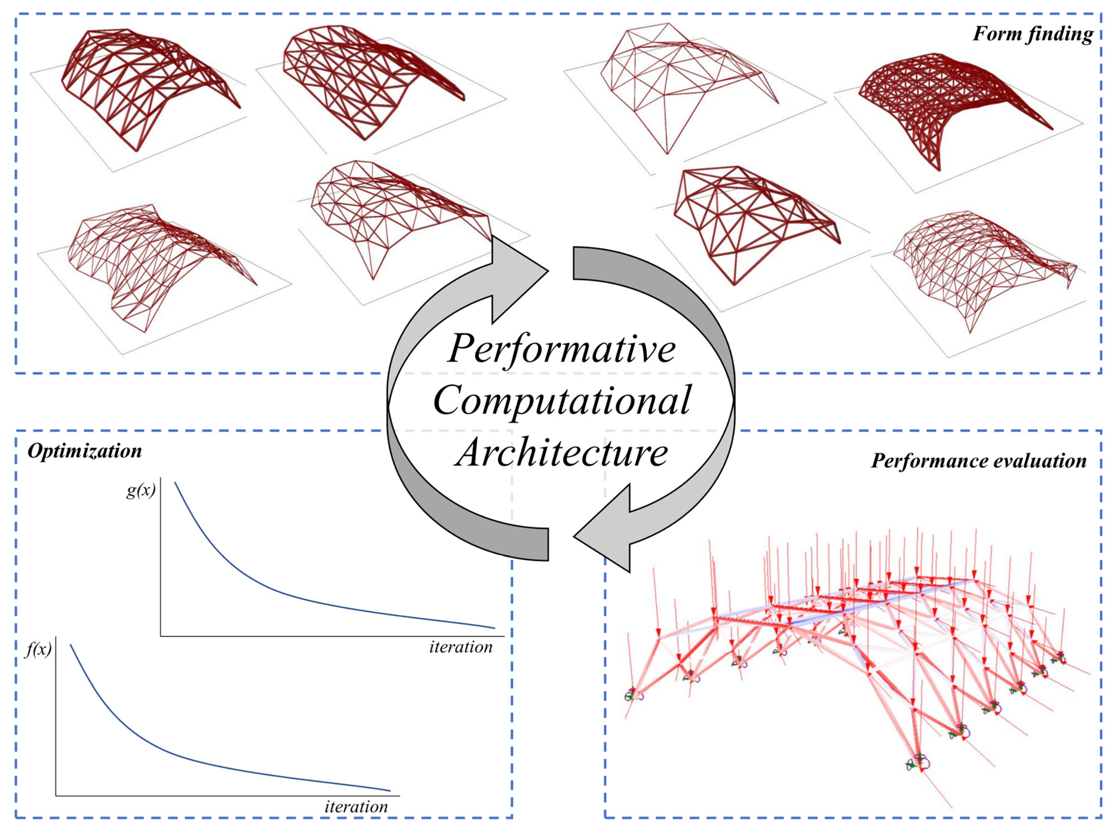
1.2. Performative Computational Architecture Framework
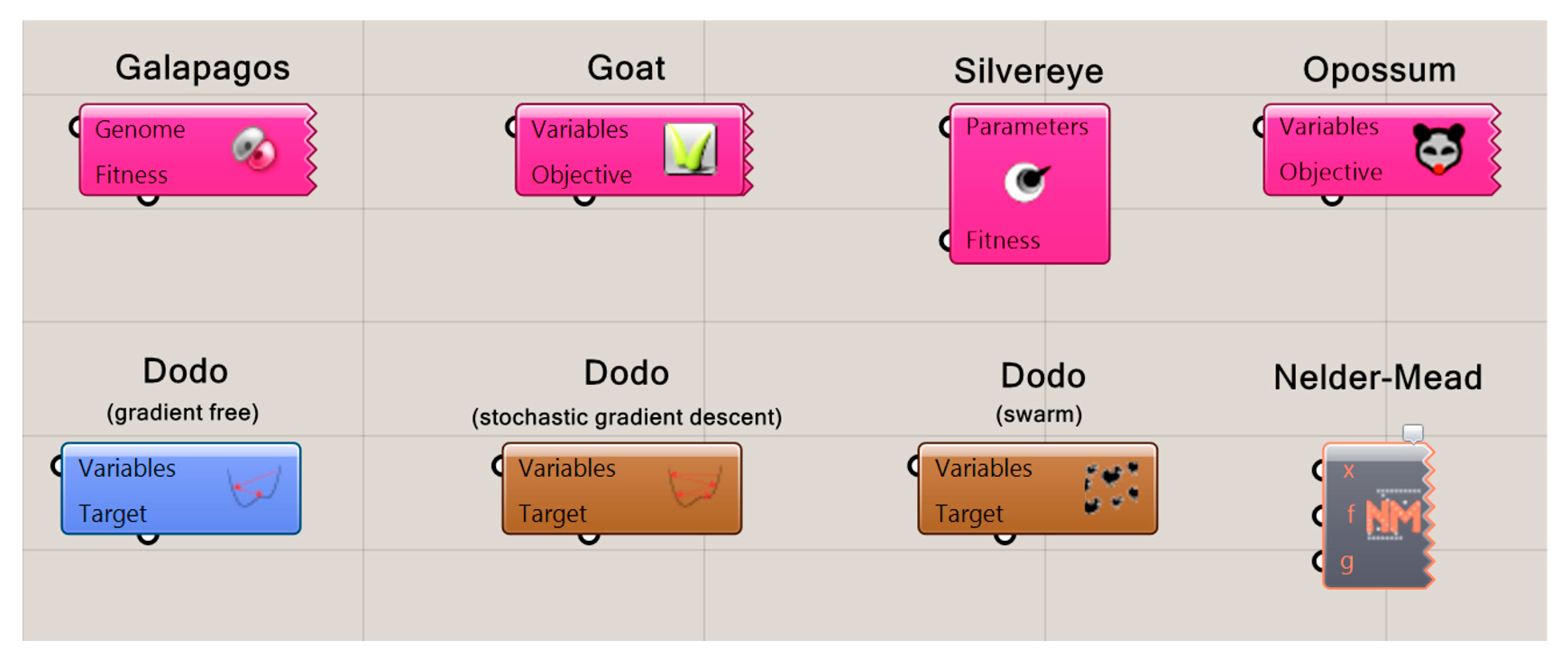
1.3. Current Optimization Tools in Grasshopper
1.3.1. Galapagos
1.3.2. Goat
1.3.3. Silvereye
1.3.4. Opossum
1.3.5. Dodo
1.3.6. Nelder–Mead Optimization
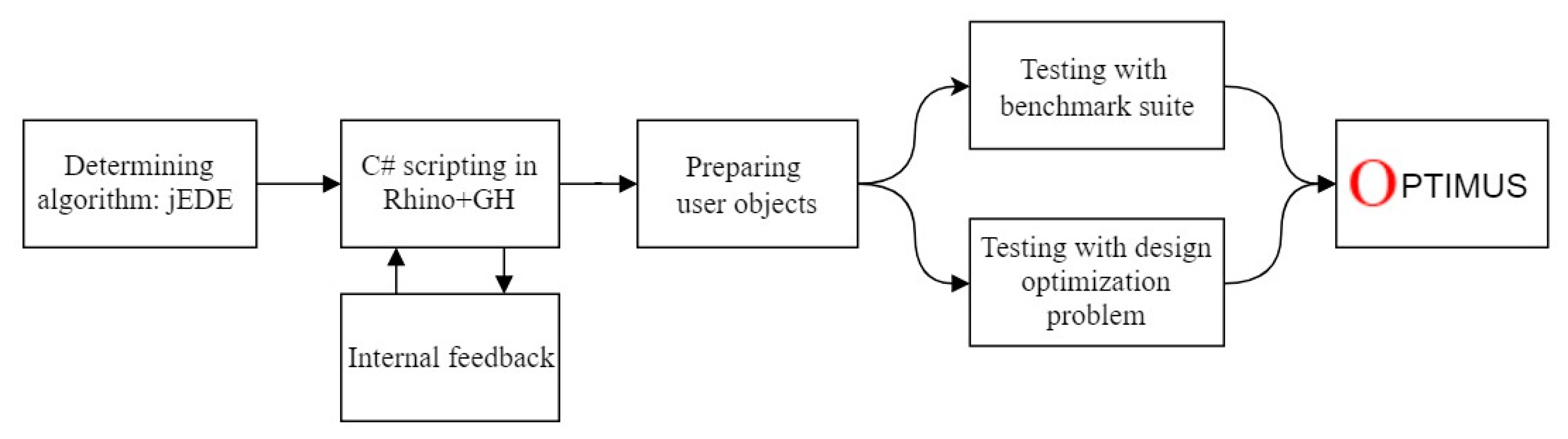
1.4. This Study: Optimus
- Supports PCA framework outlined in previous section.
- Presents the highest performance when compared to other optimization algorithms available in GH reviewed in Section 1.3.
- ○
- The performance of the Optimus is tested by benchmark suite, which consists of standard single objective unconstrained problems and some of the test problems proposed in IEEE Congress on Evolutionary Computation 2005 (CEC 2005) [44]. Problem formulations and optimization results of these benchmarks are given in Section 4.1.
- ○
- Finally, Optimus is tested with a design optimization problem. The problem formulation and optimization results are given in Section 4.2.
2. Self-Adaptive Differential Evolution Algorithm with Ensemble of Mutation Strategies
2.1. The Basic Differential Evolution
- Initialization for generating the initial target population once at the beginning.
- Reproduction with mutation for generating the mutant population by using the target population.
- Reproduction with crossover for generating the trial population by using the mutant population.
- Selection to choose the next generation among trial and target populations using one-to-one comparison. In each generation, individuals of the current population become the target population.
2.1.1. Initialization
2.1.2. Mutation
2.1.3. Crossover
2.1.4. Selection
2.2. Self-Adaptive Approach
2.3. Ensemble Approach
| Algorithm 1. The self-adaptive differential evolution algorithm with ensemble of mutation strategies. |
| 1: Set parameters g = 0, NP = 100, = 4 2: Establish initial population randomly 3: 4: Assign a mutation strategy to each individual randomly 5: 6: Evaluate population and find 7: 8: Assign CR[i] = 0.5 and F[i] = 0.9 to each individual 9: Repeat the following for each individual 10: Obtain 11: Obtain 12: Obtain 13: If , 14: If , 15: Update and 16: If the stopping criterion is not met, go to Lines 9–15 17: Else stop and return |
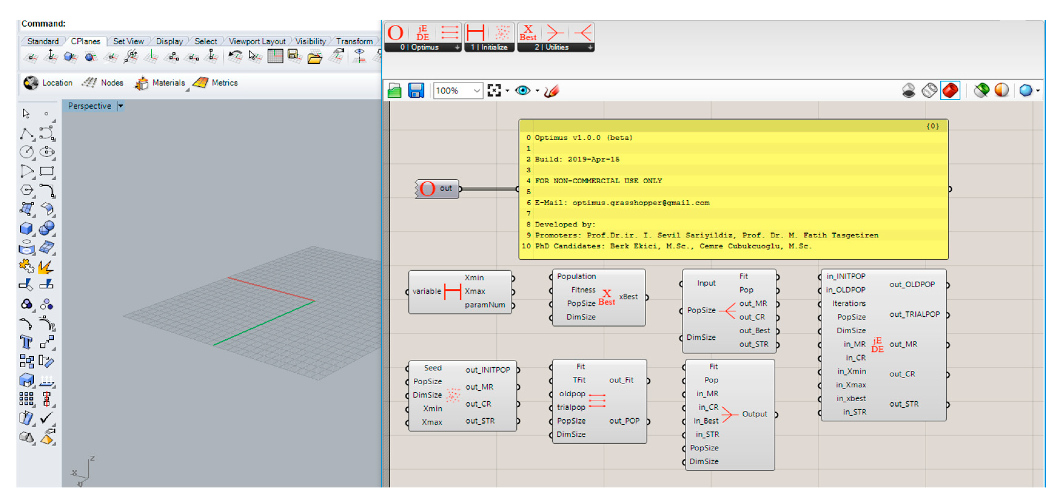
3. Optimus
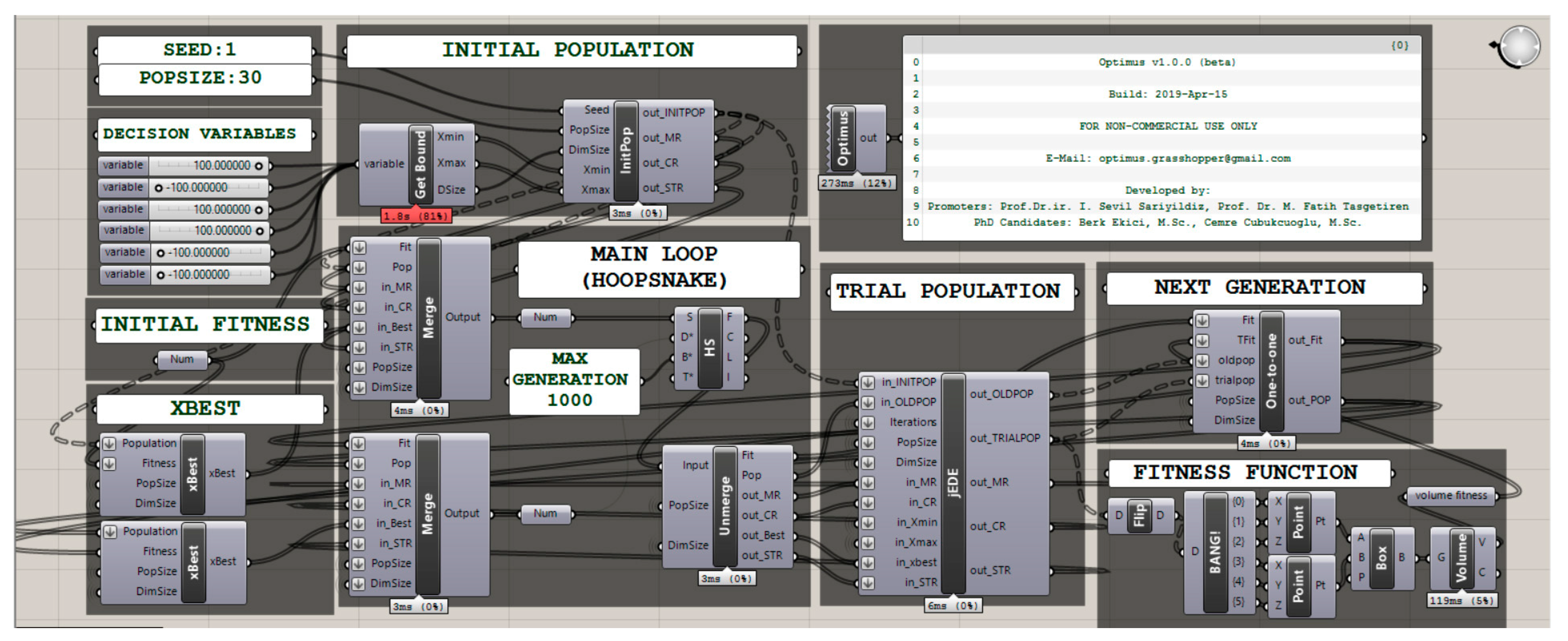
- Optimus consists of
- ReadMe (giving details about Optimus),
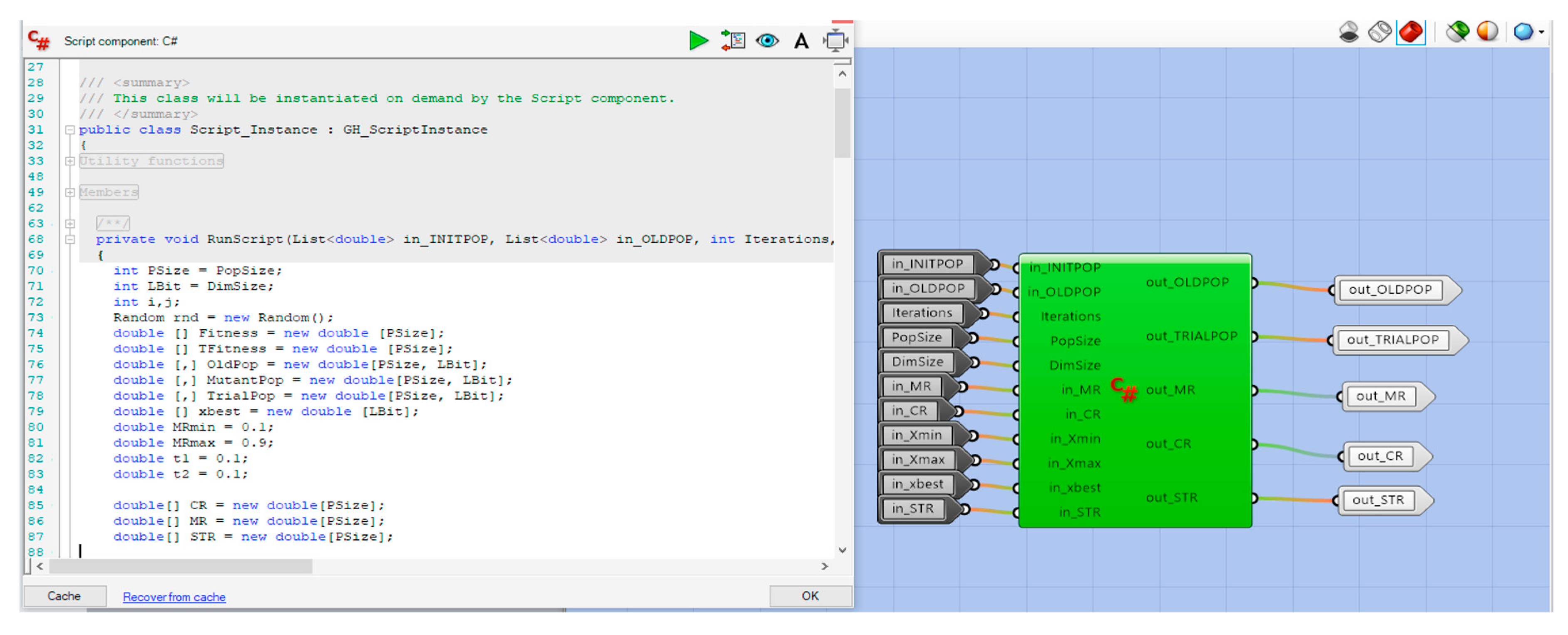
- jEDE (using jEDE algorithm, generating mutant and trial populations)
- One-to-one (enabling selection process for next generation)
- Initialize consists of
- GetBound (taking the boundaries of design variables in dimensions)
- InitPop (generating initial population for population size in dimensions)
- Utilities consists of
- xBest (finding chromosomes that has the lowest fitness value in the population)
- Merge (collecting the fitness, population, xBest and optimization parameters)
- Unmerge (separating the fitness, population, xBest and optimization parameters)
- Place GetBound on the GH canvas and connect with number sliders.
- Define the population size.
- Get InitPop for initialization using population size and output of GetBound.
- Evaluate initial fitness using the output of InitPop.
- Internalize the initial fitness.
- Place xBest on the GH canvas.
- Get Merge and connect with internalized initial fitness and outputs of InitPop and xBest.
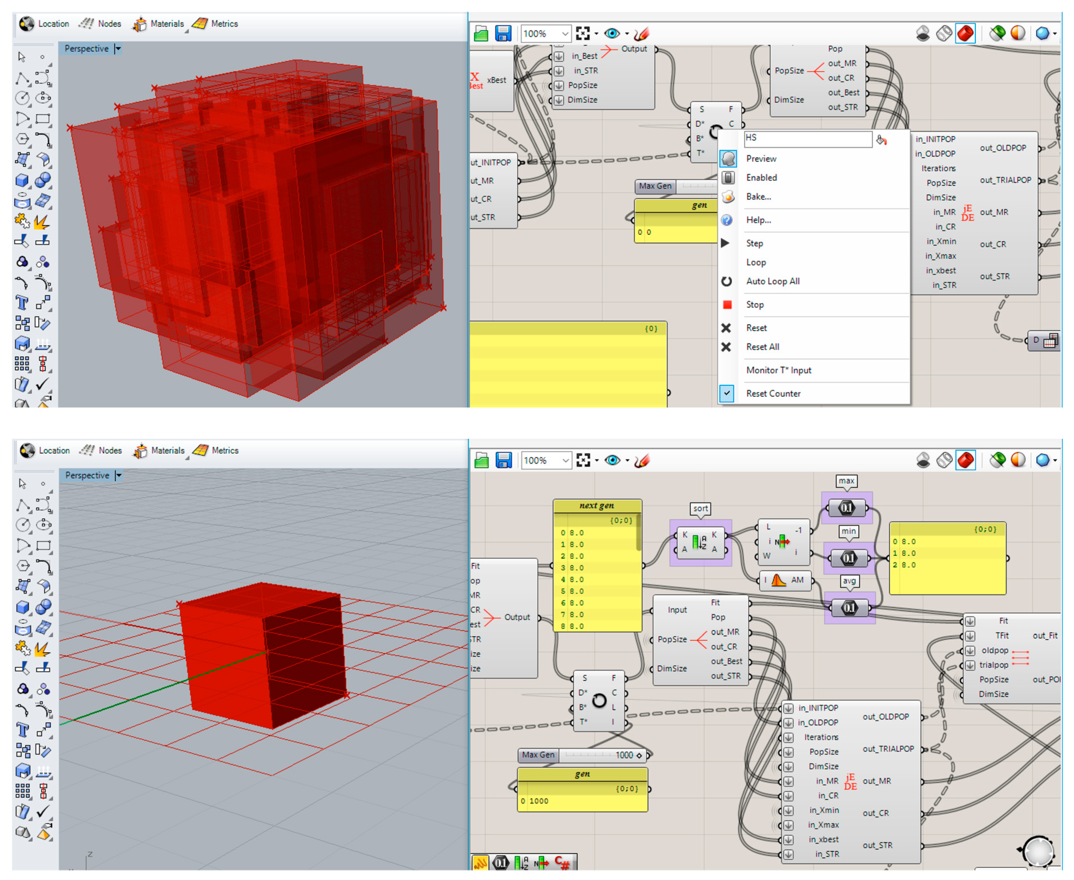
- Connect Merge with starting input (S) of HoopSnake.
- Place UnMerge on the GH canvas and connect with feedback output (F) of HoopSnake.
- Get jEDE and connect outputs of UnMerge, InitPop, GetBound.
- Evaluate trial fitness using the output of jEDE.
- Get One-to-One and connect with initial fitness, trial fitness and outputs of jEDE.
- Place xBest and connect outputs of One-to-one for updating the new best chromosome.
- Get Merge and connect outputs of jEDE, One-to-one, and xBest.
- Complete the loop by connecting the output of Merge to the data input (D) of the HoopSnake.
4. Experiments
4.1. Benchmark Suite
4.1.1. Experimental Setup and Evaluation Criteria
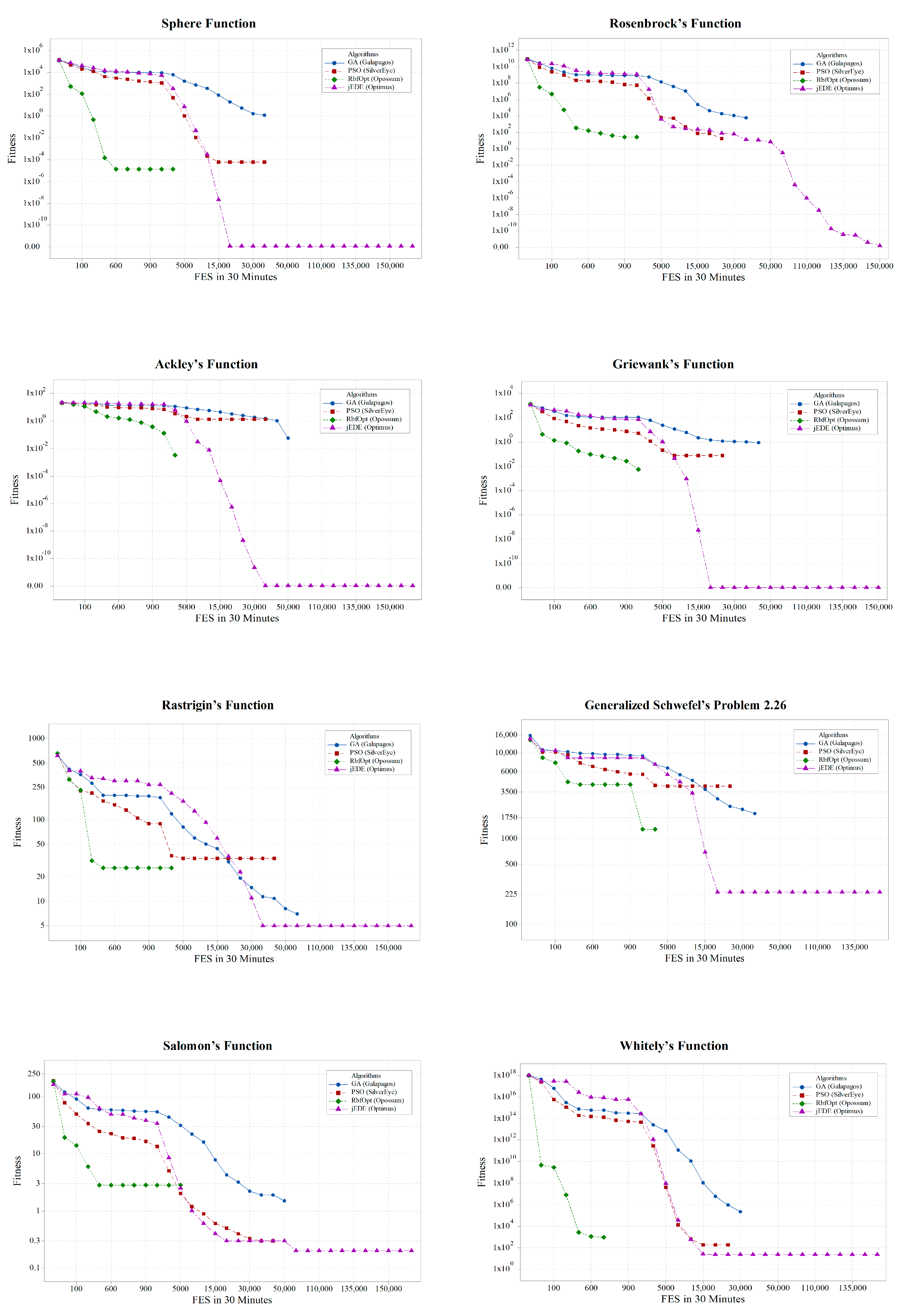
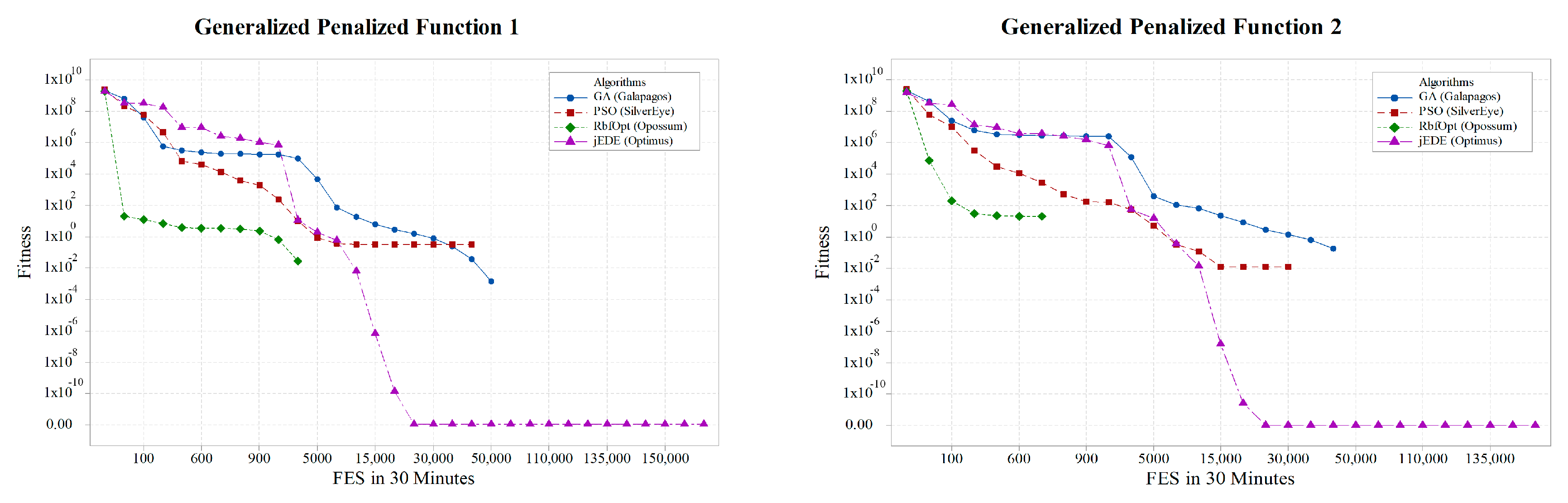
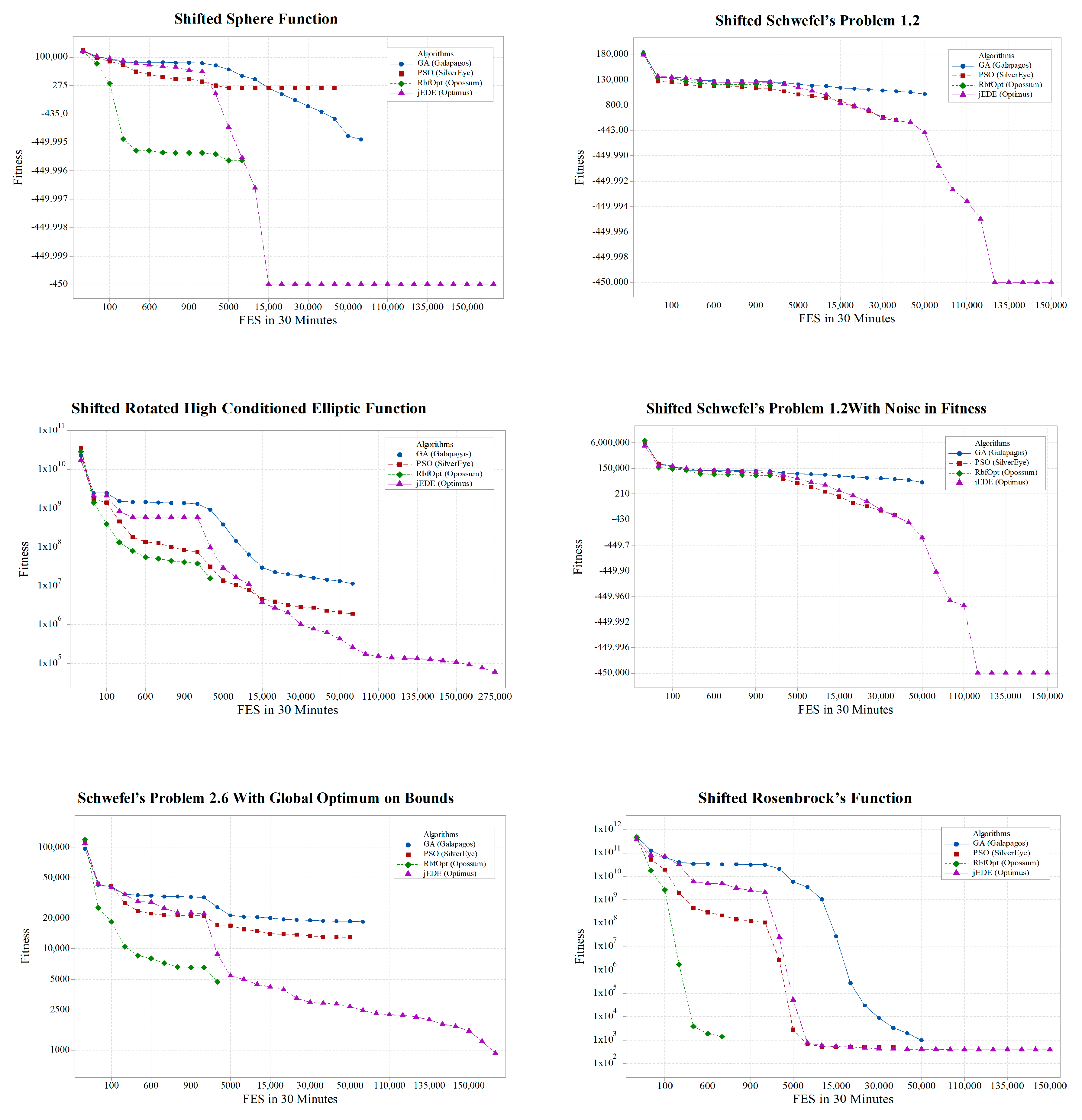
4.1.2. Experimental Results
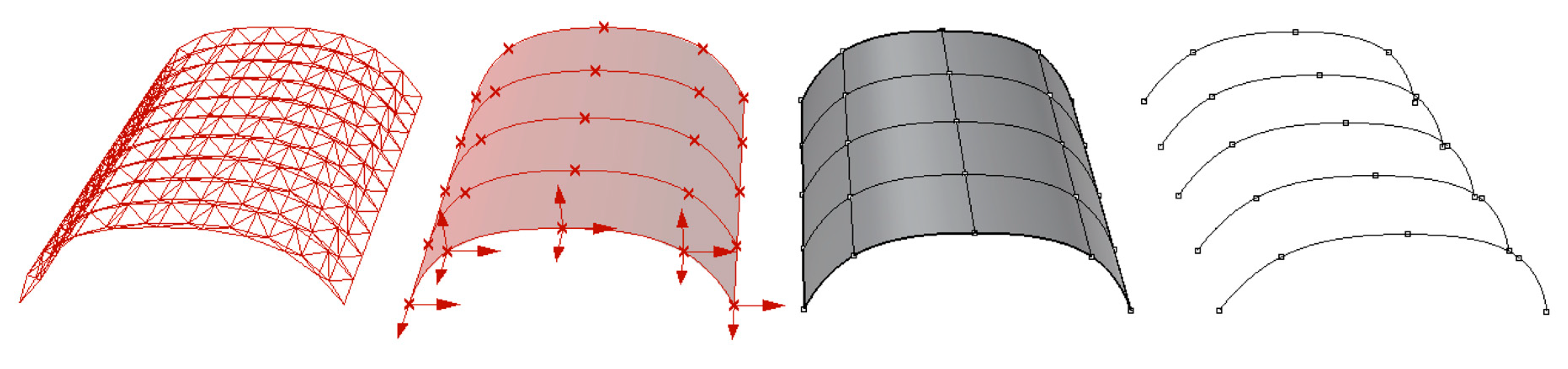
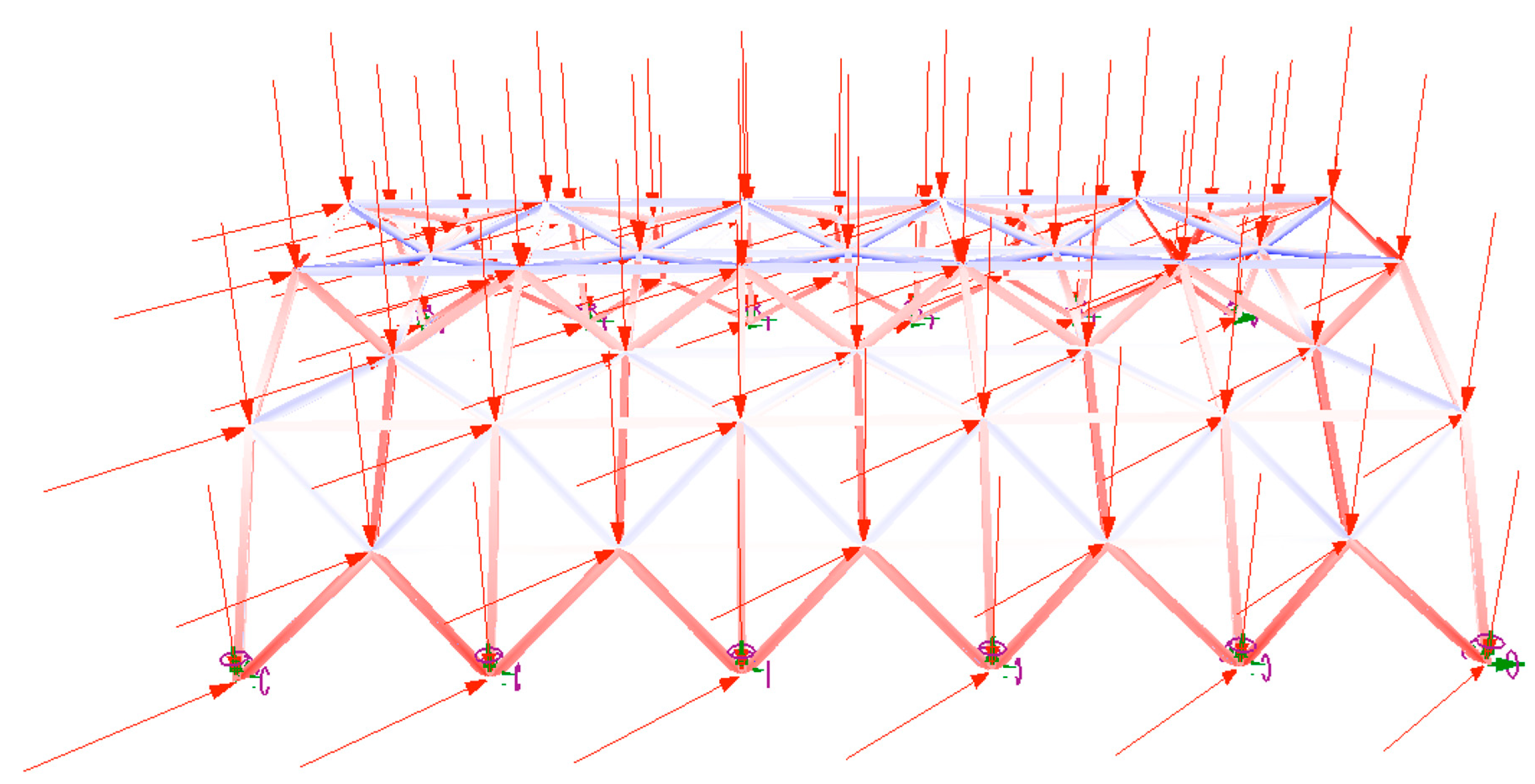
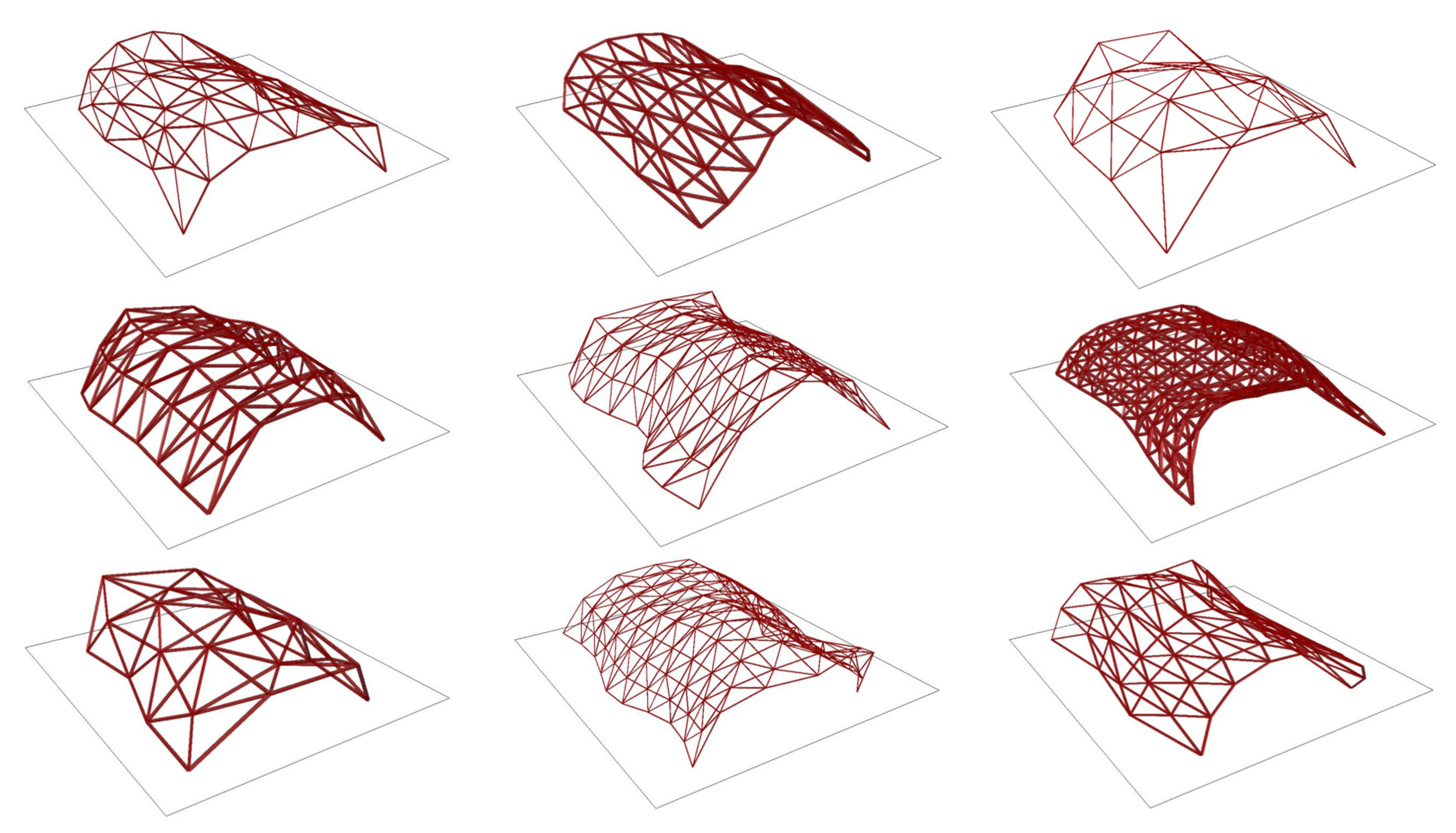
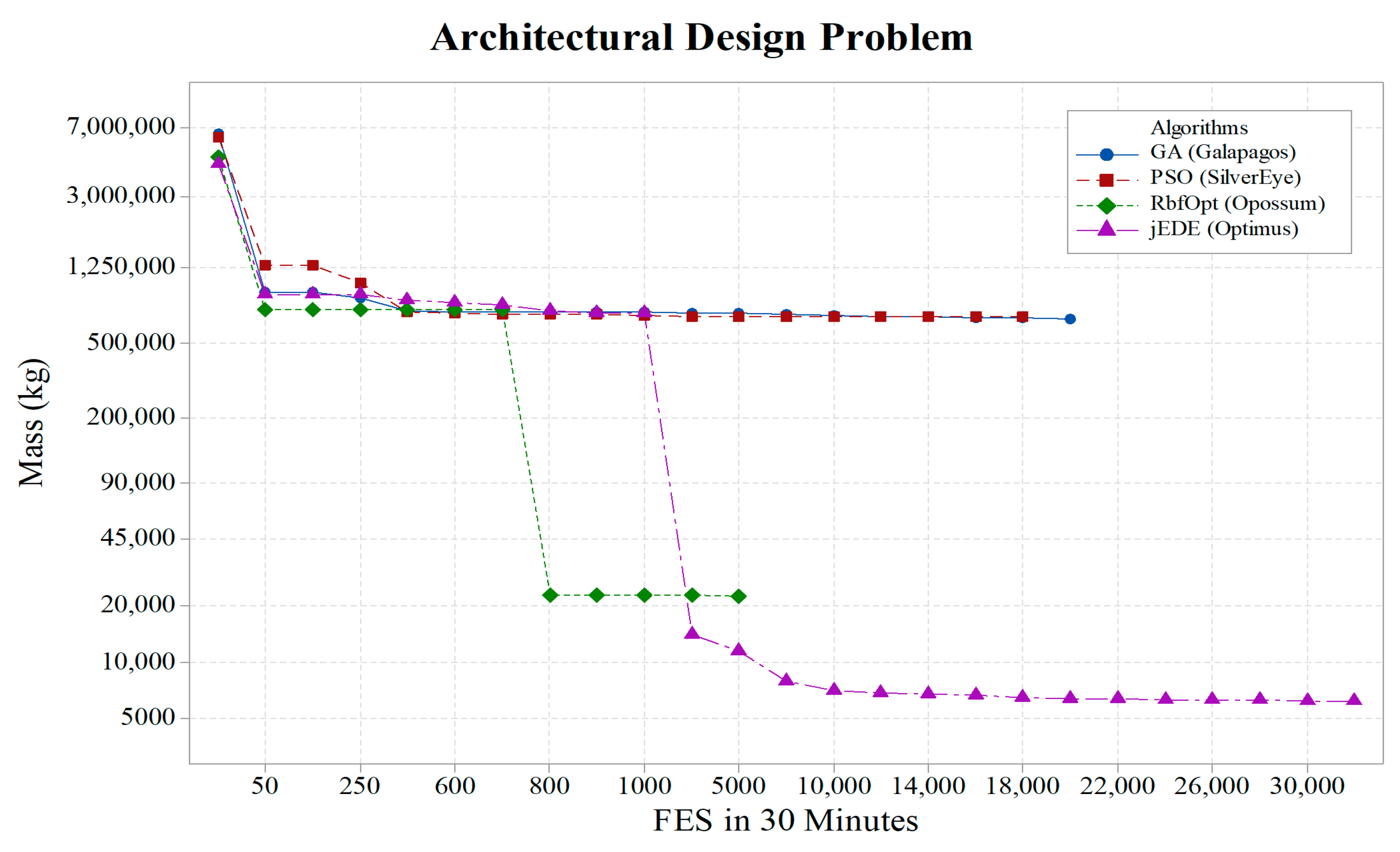
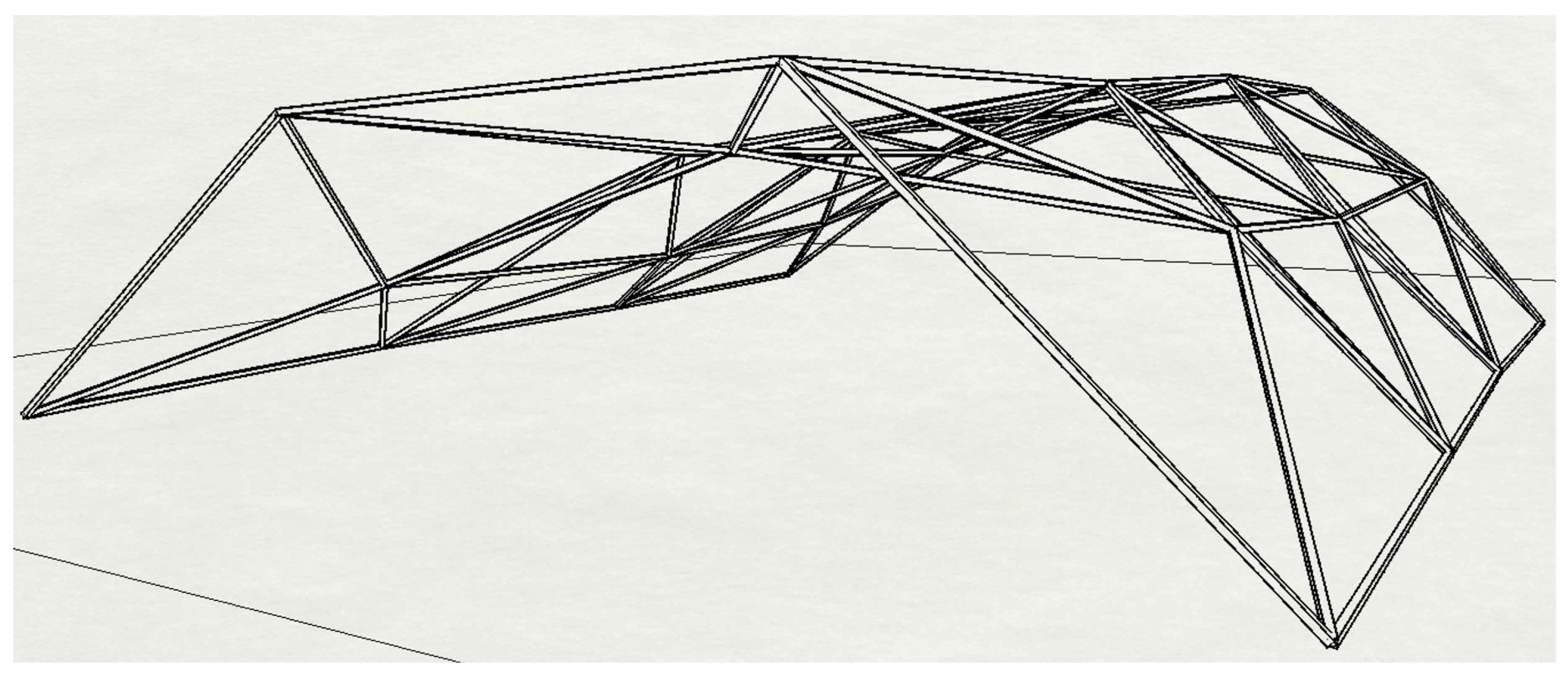
4.2. Design Optimization Problem
4.2.1. Experimental Setup and Evaluation Criteria
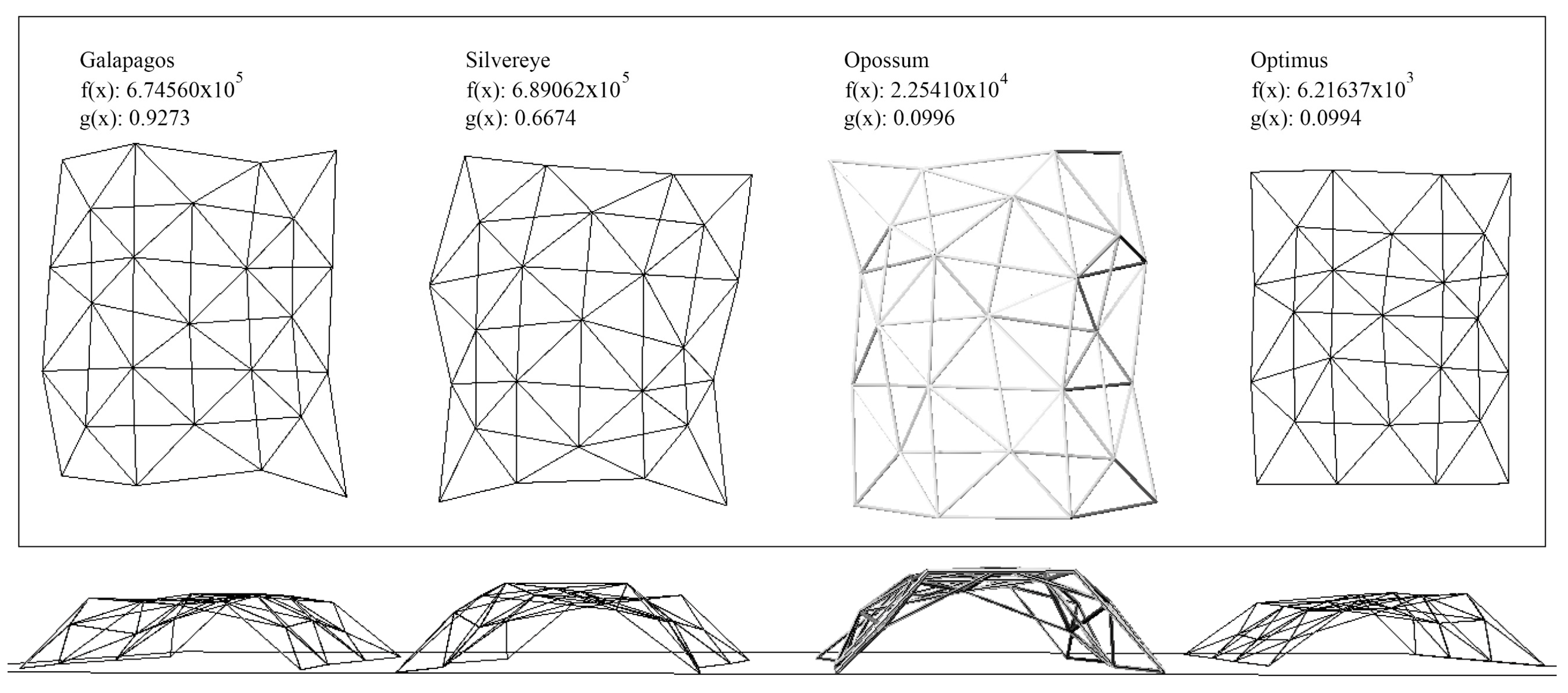
4.2.2. Design Results
5. Discussion
6. Conclusions
Supplementary Materials
Author Contributions
Funding
Acknowledgments
Conflicts of Interest
Appendix A

| : Sphere Function |
| : Rosenbrock’s Function |
| : Ackley’s Function |
| : Griewank’s Function |
| : Rastrigin’s Function |
| : Generalized Schwefel’s Problem 2.26 |
| : Salomon’s Function |
| : Whitely’s Function where |
| : Generalized Penalized Function 1 where and |
| : Generalized Penalized Function 2 |
| : Shifted Sphere Function , |
| : Shifted Schwefel’s Problem 1.2 , |
| : Shifted Rotated High Conditioned Elliptic Function , |
| : Shifted Schwefel’s Problem 1.2 With Noise in Fitness , |
| : Schwefel’s Problem 2.6 with Global Optimum on Bounds , |
| : Shifted Rosenbrock’s Function , |
| : Shifted Rotated Griewank’s Function without Bounds Initialize population in , Global optimum is outside of the initialization range, |
| : Shifted Rotated Ackley’s Function with Global Optimum on Bounds. , |
| : Shifted Rastrigin’s Function , |
| : Shifted Rotated Rastrigin’s Function . |
References
- Sariyildiz, S. Performative Computational Design, Keynote Speech. In Proceedings of the ICONARCH-I: International Congress of Architecture-I, Konya, Turkey, 15–17 November 2012. [Google Scholar]
- Ekici, B.; Cubukcuoglu, C.; Turrin, M.; Sariyildiz, I.S. Performative computational architecture using swarm and evolutionary optimisation: A review. Build. Environ. 2018, 147, 356–371. [Google Scholar] [CrossRef]
- Michalewicz, Z.; Fogel, D.B. How to Solve it: Modern Heuristics; Springer Science & Business Media: New York, NY, USA, 2013. [Google Scholar]
- Geem, Z.W.; Kim, J.H.; Loganathan, G.V. A new heuristic optimization algorithm: Harmony search. Simulation 2001, 76, 60–68. [Google Scholar] [CrossRef]
- Eberhart, R.; Kennedy, J. A New Optimizer Using Particle Swarm Theory. In Proceedings of the MHS’95. Sixth International Symposium on Micro Machine and Human Science, Nagoya, Japan, 4–6 October 1995; pp. 39–43. [Google Scholar]
- Storn, R. On the Usage of Differential Evolution for Function Optimization. In Proceedings of the North American Fuzzy Information Processing, Berkeley, CA, USA, 19–22 June 1996; pp. 519–523. [Google Scholar]
- Storn, R.; Price, K. Differential evolution—A simple and efficient heuristic for global optimization over continuous spaces. J. Glob. Optim. 1997, 11, 341–359. [Google Scholar] [CrossRef]
- Goldberg, D.E.; Holland, J.H. Genetic algorithms and machine learning. Mach. Learn. 1988, 3, 95–99. [Google Scholar] [CrossRef]
- Dorigo, M.; Gambardella, L.M. Ant colony system: A cooperative learning approach to the traveling salesman problem. IEEE Trans. Evol. Comput. 1997, 1, 53–66. [Google Scholar] [CrossRef]
- Kirkpatrick, S.; Gelatt, C.D.; Vecchi, M.P. Optimization by simulated annealing. Science 1983, 220, 671–680. [Google Scholar] [CrossRef] [PubMed]
- Coello, C.A.C.; Lamont, G.B.; van Veldhuizen, D.A. Evolutionary Algorithms for Solving Multi-Objective Problems; Springer: Berlin/Heidelberg, Germany, 2007; Volume 5. [Google Scholar]
- Wortmann, T. Genetic Evolution vs. Function Approximation: Benchmarking Algorithms for Architectural Design Optimization. J. Comput. Des. Eng. 2018, 6, 414–428. [Google Scholar] [CrossRef]
- Wortmann, T.; Waibel, C.; Nannicini, G.; Evins, R.; Schroepfer, T.; Carmeliet, J. Are Genetic Algorithms Really the Best Choice for Building Energy Optimization? In Proceedings of the Symposium on Simulation for Architecture and Urban Design, Toronto, CA, Canada, 22–24 May 2017; p. 6. [Google Scholar]
- Waibel, C.; Wortmann, T.; Evins, R.; Carmeliet, J. Building energy optimization: An extensive benchmark of global search algorithms. Energy Build. 2019, 187, 218–240. [Google Scholar] [CrossRef]
- Cichocka, J.M.; Migalska, A.; Browne, W.N.; Rodriguez, E. SILVEREYE—The Implementation of Particle Swarm Optimization Algorithm in a Design Optimization Tool. In Proceedings of the International Conference on Computer-Aided Architectural Design Futures, Istanbul, Turkey, 10–14 July 2017; pp. 151–169. [Google Scholar]
- Rutten, D. Galapagos: On the logic and limitations of generic solvers. Archit. Des. 2013, 83, 132–135. [Google Scholar] [CrossRef]
- Camporeale, P.E.; del Moyano, P.M.M.; Czajkowski, J.D. Multi-objective optimisation model: A housing block retrofit in Seville. Energy Build. 2017, 153, 476–484. [Google Scholar] [CrossRef]
- Calcerano, F.; Martinelli, L. Numerical optimisation through dynamic simulation of the position of trees around a stand-alone building to reduce cooling energy consumption. Energy Build. 2016, 112, 234–243. [Google Scholar] [CrossRef]
- Anton, I.; Tãnase, D. Informed geometries. Parametric modelling and energy analysis in early stages of design. Energy Procedia 2016, 85, 9–16. [Google Scholar] [CrossRef]
- Tabadkani, A.; Banihashemi, S.; Hosseini, M.R. Daylighting and visual comfort of oriental sun responsive skins: A parametric analysis. Build. Simul. 2018, 11, 663–676. [Google Scholar] [CrossRef]
- Lee, K.; Han, K.; Lee, J. Feasibility study on parametric optimization of daylighting in building shading design. Sustainability 2016, 8, 1220. [Google Scholar] [CrossRef]
- Fathy, F.; Sabry, H.; Faggal, A.A. External Versus Internal Solar Screen: Simulation Analysis for Optimal Daylighting and Energy Savings in an Office Space. In Proceedings of the PLEA, Edinburgh, UK, 16 August 2017. [Google Scholar]
- Lavin, C.; Fiorito, F. Optimization of an external perforated screen for improved daylighting and thermal performance of an office space. Procedia Eng. 2017, 180, 571–581. [Google Scholar] [CrossRef]
- Heidenreich, C.; Ruth, J. Parametric optimization of lightweight structures, In Proceedings of the 11th World Congress on Computational Mechanics, Barcelona, Spain, 21–25 July 2014.
- Eisenbach, P.; Grohmann, M.; Rumpf, M.; Hauser, S. Seamless Rigid Connections of Thin Concrete Shells—A Novel Stop-End Construction Technique for Prefab Elements. In Proceedings of the IASS Annual Symposia, Amsterdam, The Netherlands, 17–20 August 2015; Volume 2015, pp. 1–12. [Google Scholar]
- Almaraz, A. Evolutionary Optimization of Parametric Structures: Understanding Structure and Architecture as a Whole from Early Design Stages. Master’s Thesis, University of Coruna, La Coruña, Spain, 2015. [Google Scholar]
- Simon. Goat. 2013. Available online: https://www.food4rhino.com/app/goat (accessed on 10 July 2019).
- Johnson, S.G. The Nlopt Nonlinear-Optimization Package. Available online: https://nlopt.readthedocs.io/en/latest/ (accessed on 10 July 2019).
- Ilunga, G.; Leitão, A. Derivative-free Methods for Structural Optimization. In Proceedings of the 36th eCAADe Conference, Lodz, Poland, 19–21 September 2018. [Google Scholar]
- Austern, G.; Capeluto, I.G.; Grobman, Y.J. Rationalization and Optimization of Concrete Façade Panels. In Proceedings of the 36th eCAADe Conference, Lodz, Poland, 19–21 September 2018. [Google Scholar]
- Delmas, A.; Donn, M.; Grosdemouge, V.; Musy, M.; Garde, F. Towards Context & Climate Sensitive Urban Design: An Integrated Simulation and Parametric Design Approach. In Proceedings of the 4th International Conference On Building Energy & Environment 2018 (COBEE2018), Melbourne, Australia, 5–9 February 2018. [Google Scholar]
- Wortmann, T. Opossum: Introducing and Evaluating a Model-based Optimization Tool for Grasshopper. In Proceedings of the CAADRIA 2017, Hong Kong, China, 5–8 July 2017. [Google Scholar]
- Costa, A.; Nannicini, G. RBFOpt: An open-source library for black-box optimization with costly function evaluations. Math. Program. Comput. 2018, 10, 597–629. [Google Scholar] [CrossRef]
- Wortmann, T. Model-based Optimization for Architectural Design: Optimizing Daylight and Glare in Grasshopper. Technol. Archit. Des. 2017, 1, 176–185. [Google Scholar] [CrossRef]
- Greco, L. Dodo. 2015. Available online: https://www.food4rhino.com/app/dodo (accessed on 10 July 2019).
- Eckersley O’Callaghan’s Digital Design Group. 2013. Nelder-Mead Optimization. Available online: https://www.food4rhino.com/app/nelder-mead-optimisation-eoc (accessed on 10 July 2019).
- Lagarias, J.C.; Reeds, J.A.; Wright, M.H.; Wright, P.E. Convergence properties of the Nelder--Mead simplex method in low dimensions. SIAM J. Optim. 1998, 9, 112–147. [Google Scholar] [CrossRef]
- Wrenn, G.A. An Indirect Method for Numerical Optimization Using the Kreisselmeir-Steinhauser Function; NASA: Washington, DC, USA, 1989.
- Wolpert, D.H.; Macready, W.G. No free lunch theorems for optimization. IEEE Trans. Evol. Comput. 1997, 1, 67–82. [Google Scholar] [CrossRef]
- Attia, S.; Hamdy, M.; O’Brien, W.; Carlucci, S. Assessing gaps and needs for integrating building performance optimization tools in net zero energy buildings design. Energy Build. 2013, 60, 110–124. [Google Scholar] [CrossRef]
- Robert McNeel & Associates. Rhinoceros 3D. NURBS Modelling. 2015. Available online: https://www.rhino3d.com/ (accessed on 10 July 2019).
- Brest, J.; Greiner, S.; Boskovic, B.; Mernik, M.; Zumer, V. Self-adapting control parameters in differential evolution: A comparative study on numerical benchmark problems. IEEE Trans. Evol. Comput. 2006, 10, 646–657. [Google Scholar] [CrossRef]
- Mallipeddi, R.; Suganthan, P.N.; Pan, Q.-K.; Tasgetiren, M.F. Differential evolution algorithm with ensemble of parameters and mutation strategies. Appl. Soft Comput. 2011, 11, 1679–1696. [Google Scholar] [CrossRef]
- Suganthan, P.N.; Hansen, N.; Liang, J.J.; Deb, K.; Chen, Y.-P.; Auger, A.; Tiwari, S. Problem definitions and evaluation criteria for the CEC 2005 special session on real-parameter optimization. KanGAL Rep. 2005, 2005005, 2005. [Google Scholar]
- Blackwell, T.M.; Kennedy, J.; Poli, R. Particle swarm optimization. Swarm Intell. 2007, 1, 33–57. [Google Scholar]
- Sengupta, S.; Basak, S.; Peters, R. Particle Swarm Optimization: A survey of historical and recent developments with hybridization perspectives. Mach. Learn. Knowl. Extr. 2019, 1, 157–191. [Google Scholar] [CrossRef]
- Mirjalili, S. Genetic Algorithm. In Evolutionary Algorithms and Neural Networks; Springer: New York, NY, USA, 2019; pp. 43–55. [Google Scholar]
- Koza, J.R. Genetic Programming: On the Programming of Computers by Means of Natural Selection; MIT press: Cambridge, MA, USA, 1992; Volume 1. [Google Scholar]
- Knowles, J.; Corne, D. The Pareto Archived Evolution Strategy: A New Baseline Algorithm for Pareto Multiobjective Optimisation. In Proceedings of the Congress on Evolutionary Computation (CEC99), Washington, DC, USA, 6–9 July 1999; Volume 1, pp. 98–105. [Google Scholar]
- Pan, Q.-K.; Tasgetiren, M.F.; Liang, Y.-C. A discrete differential evolution algorithm for the permutation flowshop scheduling problem. Comput. Ind. Eng. 2008, 55, 795–816. [Google Scholar] [CrossRef]
- Venu, M.K.; Mallipeddi, R.; Suganthan, P.N. Fiber Bragg grating sensor array interrogation using differential evolution. Optoelectron. Adv. Mater. Commun. 2008, 2, 682–685. [Google Scholar]
- Varadarajan, M.; Swarup, K.S. Differential evolution approach for optimal reactive power dispatch. Appl. Soft Comput. 2008, 8, 1549–1561. [Google Scholar] [CrossRef]
- Das, S.; Konar, A. Automatic image pixel clustering with an improved differential evolution. Appl. Soft Comput. 2009, 9, 226–236. [Google Scholar] [CrossRef]
- Chatzikonstantinou, I.; Ekici, B.; Sariyildiz, I.S.; Koyunbaba, B.K. Multi-Objective Diagrid Façade Optimization Using Differential Evolution. In Proceedings of the 2015 IEEE Congress on Evolutionary Computation (CEC), Sendai, Japan, 25–28 May 2015; pp. 2311–2318. [Google Scholar]
- Cubukcuoglu, C.; Chatzikonstantinou, I.; Tasgetiren, M.F.; Sariyildiz, I.S.; Pan, Q.-K. A multi-objective harmony search algorithm for sustainable design of floating settlements. Algorithms 2016, 9, 51. [Google Scholar] [CrossRef]
- Das, S.; Suganthan, P.N. Differential evolution: A survey of the state-of-the-art. IEEE Trans. Evol. Comput. 2011, 15, 4–31. [Google Scholar] [CrossRef]
- Das, S.; Mullick, S.S.; Suganthan, P.N. Recent advances in differential evolution—an updated survey. Swarm Evol. Comput. 2016, 27, 1–30. [Google Scholar] [CrossRef]
- Tasgetiren, M.F.; Suganthan, P.N.; Pan, Q.-K.; Mallipeddi, R.; Sarman, S. An Ensemble of Differential Evolution Algorithms for Constrained Function Optimization. In Proceedings of the IEEE congress on evolutionary computation, Vancouver, BC, Canada, 24–29 July 2016; pp. 1–8. [Google Scholar]
- Hansen, N.; Ostermeier, A. Completely derandomized self-adaptation in evolution strategies. Evol. Comput. 2001, 9, 159–195. [Google Scholar] [CrossRef] [PubMed]
- Chatzikonstantinou, I. HoopSnake. 2012. Available online: https://www.food4rhino.com/app/hoopsnake (accessed on 10 July 2019).
- Miller, N. LunchBox. 2012. Available online: https://www.food4rhino.com/app/lunchbox (accessed on 10 July 2019).
- Preisinger, C.; Heimrath, M. Karamba—A toolkit for parametric structural design. Struct. Eng. Int. 2014, 24, 217–221. [Google Scholar] [CrossRef]
- Shan, S.; Wang, G.G. Survey of modeling and optimization strategies to solve high-dimensional design problems with computationally-expensive black-box functions. Struct. Multidiscip. Optim. 2010, 41, 219–241. [Google Scholar] [CrossRef]
- Coello, C.A.C. Theoretical and numerical constraint-handling techniques used with evolutionary algorithms: A survey of the state of the art. Comput. Methods Appl. Mech. Eng. 2002, 191, 1245–1287. [Google Scholar] [CrossRef]
- Tasgetiren, M.F.; Suganthan, P.N. A Multi-Populated Differential Evolution Algorithm for Solving Constrained Optimization Problem. In Proceedings of the 2006 IEEE International Conference on Evolutionary Computation, Vancouver, BC, Canada, 16–21 July 2006; pp. 33–40. [Google Scholar]
- Coit, D.W.; Smith, A.E. Penalty guided genetic search for reliability design optimization. Comput. Ind. Eng. 1996, 30, 895–904. [Google Scholar] [CrossRef]
- Deb, K. An efficient constraint handling method for genetic algorithms. Comput. Methods Appl. Mech. Eng. 2000, 186, 311–338. [Google Scholar] [CrossRef]
- Haimes, Y.V. On a bicriterion formulation of the problems of integrated system identification and system optimization. IEEE Trans. Syst. Man. Cybern. 1971, 1, 296–297. [Google Scholar]
- Mallipeddi, R.; Suganthan, P.N. Ensemble of constraint handling techniques. IEEE Trans. Evol. Comput. 2010, 14, 561–579. [Google Scholar] [CrossRef]


| Notation | Function |
|---|---|
| Sphere Function | |
| Rosenbrock’s Function | |
| Ackley’s Function | |
| Griewank’s Function | |
| Rastrigin’s Function | |
| Generalized Schwefel’s Problem 2.26 | |
| Salomon’s Function | |
| Whitely’s Function | |
| Generalized Penalized Function 1 | |
| Generalized Penalized Function 2 | |
| Shifted Sphere Function | |
| Shifted Schwefel’s Problem 1.2 | |
| Shifted Rotated High Conditioned Elliptic Function | |
| Shifted Schwefel’s Problem 1.2 With Noise in Fitness | |
| Schwefel’s Problem 2.6 With Global Optimum on Bounds | |
| Shifted Rosenbrock’s Function | |
| Shifted Rotated Griewank’s Function without Bounds | |
| Shifted Rotated Ackley’s Function with Global Optimum on Bounds | |
| Shifted Rastrigin’s Function | |
| Shifted Rotated Rastrigin’s Function |
| Optimus_jEDE | Opossum_RBFOpt | SilverEye_PSO | Galapagos_GA | Optimal | ||
|---|---|---|---|---|---|---|
| 0.0000000 | 1.4000000 | 5.9000000 | 1.1709730 | 0 | ||
| 0.0000000 | 5.8000000 | 2.7057298 | 4.4052130 | |||
| 0.0000000 | 3.6400000 | 5.4171618 | 2.7928586 | |||
| Std.Dev. | 0.0000000 | 1.8039956 | 1.0820072 | 1.1492298 | ||
| FES | 194,520 | 3225 | 31,560 | 34,260 | ||
| 0.0000000 | 2.7485056 | 1.6689612 | 6.0863438 | 0 | ||
| 3.9866240 | 2.1030328 | 5.8965910 | 2.2859534 | |||
| 2.3919744 | 9.0892522 | 1.3859753 | 1.3060872 | |||
| Std.Dev. | 1.9530389 | 7.1919037 | 2.2886020 | 6.7095472 | ||
| FES | 149,460 | 882 | 26,700 | 35,070 | ||
| 0.0000000 | 3.3550000 | 1.3404210 | 5.7470000 | 0 | ||
| 1.3404210 | 2.4098540 | 3.7340120 | 1.0270860 | |||
| 2.6808420 | 1.3795174 | 2.2482728 | 4.8037520 | |||
| Std.Dev. | 5.3616840 | 8.5713298 | 9.1850828 | 4.0392221 | ||
| FES | 206,370 | 1447 | 38,490 | 28,710 | ||
| 0.0000000v | 1.5840000 | 3.2081000 | 3.4407200 | 0 | ||
| 0.0000000 | 1.7086000 | 2.6292800 | 1.0657060 | |||
| 0.0000000 | 7.6638000 | 1.2049020 | 8.2474220 | |||
| Std.Dev. | 0.0000000 | 5.6121253 | 8.1064770 | 2.6131521 | ||
| FES | 151,110 | 1089 | 26,610 | 37,410 | ||
| 4.9747950 | 2.5870757 | 3.3829188 | 7.0535550 | 0 | ||
| 2.3879007 | 4.1789542 | 6.1687356 | 2.9072445 | |||
| 1.3332448 | 3.6218407 | 4.8355074 | 1.5404780 | |||
| Std.Dev. | 6.7363920 | 5.4349940 | 1.1424086 | 9.1077975 | ||
| FES | 206,520 | 4149 | 37,650 | 51,480 | ||
| 2.3687705 | 1.2877414 | 4.1089621 | 1.9550066 | 0 | ||
| 4.7375372 | 4.0111803 | 6.1589437 | 2.7977670 | |||
| 4.0269072 | 2.7169368 | 5.2658793 | 2.3201102 | |||
| Std.Dev. | 9.4750668 | 8.8809862 | 6.6677783 | 2.8681876 | ||
| FES | 148,140 | 1487 | 27,210 | 35,940 | ||
| 1.9987300 | 2.8070190 | 2.9987300 | 1.4998750 | 0 | ||
| 4.9987300 | 4.3000810 | 4.9987300 | 2.8375760 | |||
| 3.1987300 | 3.4413810 | 3.7987300 | 2.0682340 | |||
| Std.Dev. | 1.1661904 | 5.6623101 | 7.4833148 | 6.1557512 | ||
| FES | 201,720 | 4769 | 38,640 | 51,360 | ||
| 2.3704633 | 9.6592754 | 1.8455490 | 2.3632742 | 0 | ||
| 2.4040716 | 1.6904059 | 6.2776811 | 5.5055000 | |||
| 1.0789137 | 1.2610498 | 4.0698894 | 2.7440867 | |||
| Std.Dev. | 7.4951993 | 2.6984398 | 1.6923390 | 2.2575944 | ||
| FES | 146,640 | 728 | 23,250 | 29,730 | ||
| 0.0000000 | 2.9057000 | 3.1283800 | 1.4510000 | 0 | ||
| 0.0000000 | 9.0392970 | 1.3487570 | 1.7632000 | |||
| 0.0000000 | 2.8243854 | 6.7680180 | 6.0638000 | |||
| Std.Dev. | 0.0000000 | 3.1774566 | 4.2868737 | 6.0403379 | ||
| FES | 203,880 | 1394 | 39,420 | 57,720 | ||
| 0.0000000 | 2.0400434 | 1.0000000 | 1.8037300 | 0 | ||
| 1.0987000 | 2.8693232 | 9.3079800 | 2.7208440 | |||
| 2.1974000 | 2.5384324 | 2.2552480 | 1.0041520 | |||
| Std.Dev. | 4.3948000 | 3.4851206 | 3.5679494 | 9.4298611 | ||
| FES | 148,380 | 639 | 29,040 | 41,520 | ||
| −4.5000000 | −4.4999898 | 2.6232595 | −4.4995998 | −450 | ||
| −4.5000000 | −4.4999478 | 8.0377273 | −4.4988406 | |||
| −4.5000000 | −4.4999680 | 4.0824562 | −4.4992015 | |||
| Std.Dev. | 0.0000000 | 1.4829922 | 2.9460423 | 3.0428108 | ||
| FES | 198,060 | 6156 | 45,580 | 66,180 | ||
| −4.5000000 | 3.4590652 | −3.8035693 | 6.8476195 | −450 | ||
| −4.5000000 | 4.7978174 | 5.2590674 | 1.2302281 | |||
| −4.5000000 | 4.3226072 | −1.2838464 | 1.0174618 | |||
| Std.Dev. | 0.0000000 | 4.9030645 | 3.3183646 | 1.8557926 | ||
| FES | 146,010 | 1061 | 33,840 | 50,160 | ||
| 6.0045376 | 1.5561000 | 1.9264000 | 1.1250000 | −450 | ||
| 2.4850013 | 7.5084000 | 8.0820000 | 2.7772000 | |||
| 1.2857393 | 3.7380600 | 4.5525000 | 1.7212200 | |||
| Std.Dev. | 6.4175884 | 2.0647812 | 2.0206526 | 5.6281541 | ||
| FES | 205,260 | 1293 | 48,030 | 66,000 | ||
| −4.5000000 | 2.8373782 | −4.2715712 | 7.8877685 | −450 | ||
| −4.5000000 | 3.9404224 | 4.0484178 | 1.1191542 | |||
| −4.5000000 | 3.2359668 | 5.1724092 | 9.4535270 | |||
| Std.Dev. | 0.0000000 | 4.0412734 | 1.7663033 | 1.2966977 | ||
| FES | 147,240 | 1055 | 35,610 | 53,520 | ||
| 9.3362001 | 4.7527012 | 7.5856684 | 1.8506721 | -310 | ||
| 2.5603668 | 5.8813877 | 1.2910221 | 2.4057172 | |||
| 2.0333032 | 5.3824799 | 9.4390617 | 2.0151105 | |||
| Std.Dev. | 570.1512256 | 438.2070353 | 2031.289127 | 2004.100331 | ||
| FES | 195,720 | 1891 | 47,550 | 67,560 | ||
| 3.9000000 | 1.4168473 | 5.0073093 | 9.7856127 | 390 | ||
| 3.9398662 | 1.3904779 | 4.1540000 | 9.6995775 | |||
| 3.9159465 | 8.7212119 | 9.8402870 | 5.6395846 | |||
| Std.Dev. | 1.9530389 | 4.6035484 | 1.5972516 | 3.5378379 | ||
| FES | 148,260 | 687 | 33,540 | 48,810 | ||
| 4.5162886 | 4.5162896 | 5.8669417 | 4.5172240 | -180 | ||
| 4.5162886 | 4.5162985 | 7.2432580 | 4.5290168 | |||
| 4.5162886 | 4.5162936 | 6.5251090 | 4.5222540 | |||
| Std.Dev. | 0.0000000 | 3.1911420 | 5.4380701 | 4.7496031 | ||
| FES | 200,820 | 10,108 | 42,060 | 58,290 | ||
| −1.1905178 | −1.1910166 | −1.1901775 | −1.1940297 | -140 | ||
| −1.1902135 | −1.1876717 | −1.1892500 | −1.1906700 | |||
| −1.1903319 | −1.1889866 | −1.1899553 | −1.1919711 | |||
| Std.Dev. | 1.0538581 | 1.1070562 | 3.5483336 | 1.4127484 | ||
| FES | 149,670 | 2018 | 35,580 | 52,020 | ||
| −3.1706554 | −2.5827181 | −2.3690804 | −3.1677970 | -330 | ||
| −3.1209075 | −2.3567358 | −1.6682751 | −3.1164785 | |||
| −3.1527462 | −2.4625749 | −1.8917798 | −3.1499413 | |||
| Std.Dev. | 1.7117897 | 8.0334497 | 2.5285354 | 1.8617799 | ||
| FES | 212,160 | 5577 | 47,610 | 67,560 | ||
| −2.7030257 | −2.3528777 | −1.3299956 | 4.0215414 | -330 | ||
| −2.2751946 | −1.3298172 | −8.1262211 | 1.8543670 | |||
| −2.5139841 | −1.8578676 | −1.0572303 | 1.1181316 | |||
| Std.Dev. | 1.4307998 | 3.9394042 | 1.8528544 | 5.7458318 | ||
| FES | 146,820 | 1192 | 35,220 | 53,070 |
| Notation | Design Parameter | Min | Max | Type |
|---|---|---|---|---|
| x1–x13 | Coordinates of control points in axis 1 | −2.00 | 2.00 | Continues |
| x14–x26 | Coordinates of control points in axis 2 | −2.00 | 2.00 | Continues |
| x27–x39 | Coordinates of control points in axis 3 | −2.00 | 2.00 | Continues |
| x40–x52 | Coordinates of control points in axis 4 | −2.00 | 2.00 | Continues |
| x53–x65 | Coordinates of control points in axis 5 | −2.00 | 2.00 | Continues |
| x66 | Division amount on u direction | 3 | 10 | Discrete |
| x67 | Division amount on v direction | 3 | 10 | Discrete |
| x68 | Depth of the truss | 0.50 | 1.00 | Continues |
| x69 | Height of the cross-section | 10.00 | 30.00 | Continues |
| x70 | Upper and lower width of the cross-section | 10.00 | 30.00 | Continues |
| Optimus jEDE | Opossum RBFOpt | Silve Eye_PSO | Galapagos GA | ||
|---|---|---|---|---|---|
| Design problem | 6.21637 | 2.25410 | 6.89062 | 6.74560 | |
| 0.0994 | 0.0996 | 0.6674 | 0.9273 | ||
| FES | 31,800 | 5102 | 17,100 | 19,000 |
© 2019 by the authors. Licensee MDPI, Basel, Switzerland. This article is an open access article distributed under the terms and conditions of the Creative Commons Attribution (CC BY) license (http://creativecommons.org/licenses/by/4.0/).
Share and Cite
Cubukcuoglu, C.; Ekici, B.; Tasgetiren, M.F.; Sariyildiz, S. OPTIMUS: Self-Adaptive Differential Evolution with Ensemble of Mutation Strategies for Grasshopper Algorithmic Modeling. Algorithms 2019, 12, 141. https://doi.org/10.3390/a12070141
Cubukcuoglu C, Ekici B, Tasgetiren MF, Sariyildiz S. OPTIMUS: Self-Adaptive Differential Evolution with Ensemble of Mutation Strategies for Grasshopper Algorithmic Modeling. Algorithms. 2019; 12(7):141. https://doi.org/10.3390/a12070141
Chicago/Turabian StyleCubukcuoglu, Cemre, Berk Ekici, Mehmet Fatih Tasgetiren, and Sevil Sariyildiz. 2019. "OPTIMUS: Self-Adaptive Differential Evolution with Ensemble of Mutation Strategies for Grasshopper Algorithmic Modeling" Algorithms 12, no. 7: 141. https://doi.org/10.3390/a12070141
APA StyleCubukcuoglu, C., Ekici, B., Tasgetiren, M. F., & Sariyildiz, S. (2019). OPTIMUS: Self-Adaptive Differential Evolution with Ensemble of Mutation Strategies for Grasshopper Algorithmic Modeling. Algorithms, 12(7), 141. https://doi.org/10.3390/a12070141