Total Optimization of Energy Networks in a Smart City by Multi-Population Global-Best Modified Brain Storm Optimization with Migration


Abstract
:1. Introduction
- -
- A proposal of a new evolutionary computation method, namely MP-GMBSO with migration, in order to realize improvement of quality of solution,
- -
- An application of MP-GMBSO with migration-based method to total optimization of energy networks in a smart city,
- -
- Verification of efficacy of the conventional GMBSO based method for total optimization of smart city by comparing with the conventional DEEPSO, BSO, MBSO, and GBSO based methods,
- -
- Verification of efficacy of the proposed MP-GMBSO based method with migration for total optimization of smart city by comparing with the original GMBSO (GMBSO with one population) based method, and the MP-GMBSO based methods with various interaction model (only using migration, only using abest, and using both migration and abest), various policies, various topologies, various numbers of individuals, and various numbers of sub-populations,
- -
- It is verified that quality of solution is the most improved by the proposed MP-GMBSO with migration-based method using the ring topology with 16 sub-populations and 320 individuals, and the W-B policy (the worst individual of a sub-population is substituted by the best individual of other sub-populations) among all of multi-population parameters.
2. Smart City Model
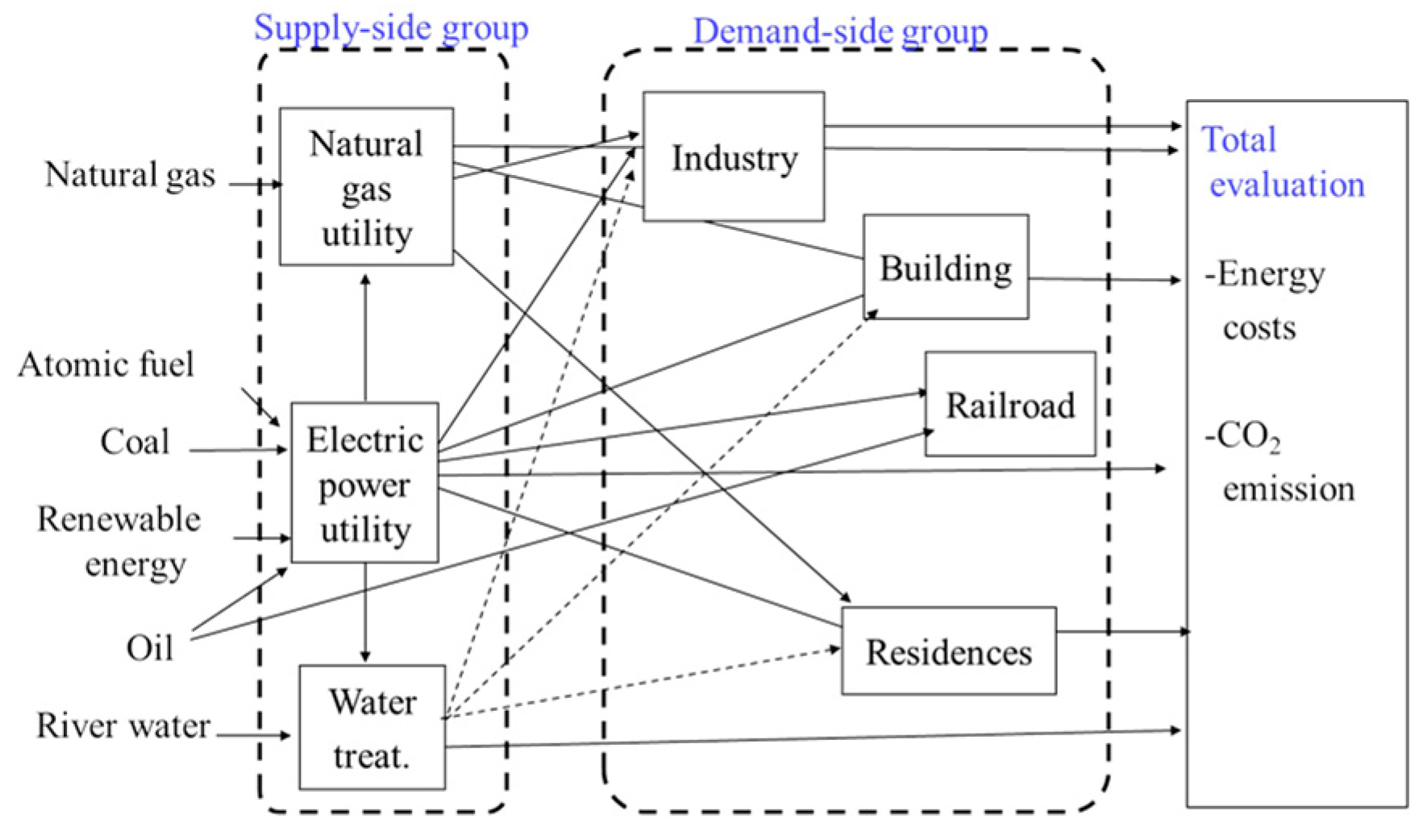
2.1. A Summary of the Whole Smart City Model
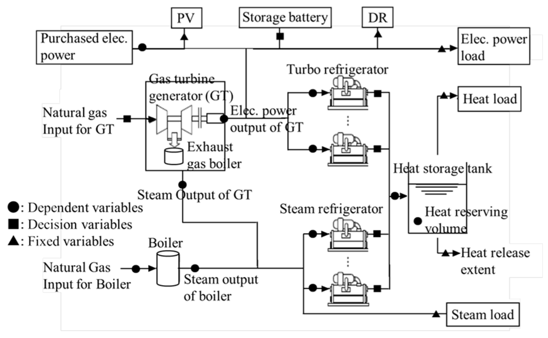
2.2. Sector Models in the Supply-Side Group
2.3. Sector Models in the Demand-Side Group
3. Problem Formulation of Total Optimization of Energy Networks in a Smart City
3.1. Decision Variables
3.2. Objective Function
3.3. Constraints
- (1)
- Energy balances: Electric power, hot and cold heat, and steam energy balances are considered. These energy balances are expressed using the following equation:where is a balance equation of energy in sector , is a startup or shutdown status of a facility for decision variable , and is an input or output real value of a facility for decision variable , is the number of energies in sector , and is the number of decision variables.
- (2)
- Facility characteristics: Efficiency functions of facilities, and upper and lower bounds of various facilities in each sector can be expressed using the following equation:where is an efficiency function of facility, or upper and lower bounds of facility of sector , and is the number of facilities in sector .Efficiency of facility should be sometimes expressed with nonlinear functions. Hence, the problem is considered as one of mixed-integer nonlinear optimization problems (MINLPs) and evolutionary computation methods should be utilized in order to treat the problem.
4. The Proposed Multi-Population Global-Best Modified Brain Storm Optimization with Migration
4.1. Overview of BSO
- Step 1
- Initialization: Randomly generate individuals and calculate the objective function values of individuals.
- Step 2
- Clustering: The k-means method is applied to divide individuals into clusters.
- Step 3
- Generation of New individual: One or two clusters are randomly selected, and new individuals are generated.
- Step 4
- Selection of individuals: Individuals which are newly generated are compared with the current individuals which have the same individual indices of the newly generated individuals. Keep the better ones and the individuals are stored as the current individuals.
- Step 5
- Evaluation of individuals: The newly stored individuals are evaluated.
- Step 6
- The procedure can be stopped and go to Step 7 when the iteration number reaches the maximum iteration number which is pre-determined. Otherwise, go to Step 2 and repeat the procedures.
- Step 7
- The objective function value and the finally obtained variables are output as a set of the final solution.
4.1.1. Clustering of BSO
- Step 2-1
- Clustering: The k-means algorithm is applied to divide individuals into clusters.
- Step 2-2
- A value is randomly generated in random (1,0).
- Step 2-3
- Individuals are ranked in each cluster.If (a pre-determined probability),the best individual is set as the cluster center in each cluster,Otherwise,One individual is randomly selected in each cluster, and the selected individual is set as the cluster center.
4.1.2. Generation of New Individual of BSO
4.2. Overview of MBSO
4.2.1. Clustering of MBSO
- Step 1
- different individuals are randomly selected from the current generation as group centers of groups.
- Step 2
- Calculate distances between the individuals and each group center. Distances to all group centers are compared. The individuals are assigned to the closest group.
- Step 3
- Individuals are ranked in each cluster.If (a pre-determined probability),the best individual is set as the cluster center in each cluster,Otherwise,One individual is randomly selected in each cluster, and the selected individual is set as the cluster center.
4.2.2. Generation of New Individuals in MBSO
4.3. Overview of GBSO
4.3.1. Clustering
- Step 1
- Individuals are ranked using calculated values of the objective function.
- Step 2
- individuals are divided into groups using (8).where, is the selected group number of individual , is a ranking of individual .
4.3.2. Generation of New Individuals of GBSO
4.4. Overview of GMBSO
- Step 1
- Initialization: individuals are randomly generated and evaluated.
- Step 2
- Clustering: individuals are divided into clusters by Fitness-based grouping explained in 4.3.
- Step 3
- Generation of new individuals: Randomly select one cluster or two clusters. When the condition (9) is satisfied, information of “gbest” is applied to using (11). Then, new individuals are generated using Equation (7) explained in 4.2.
- Step 4
- Selection: The individuals which are newly generated are compared with the current individuals with the same individual indices. The better one is kept and stored as the current individual.
- Step 5
- Evaluation: The individuals are evaluated.
- Step 6
- The procedure can be stopped and go to Step 7 if the number of current iteration reaches the maximum number of iteration which is pre-determined. Otherwise, go to Step 2 and repeat the procedures.
- Step 7
- The objective function value and the finally obtained variables are output as a final solution.
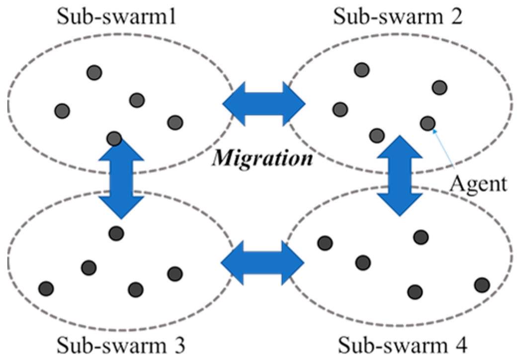
4.5. Overview of the Proposed MP-GMBSO
- -
- The number of sub-populations: the number of sub-populations which performs GMBSO independently.
- -
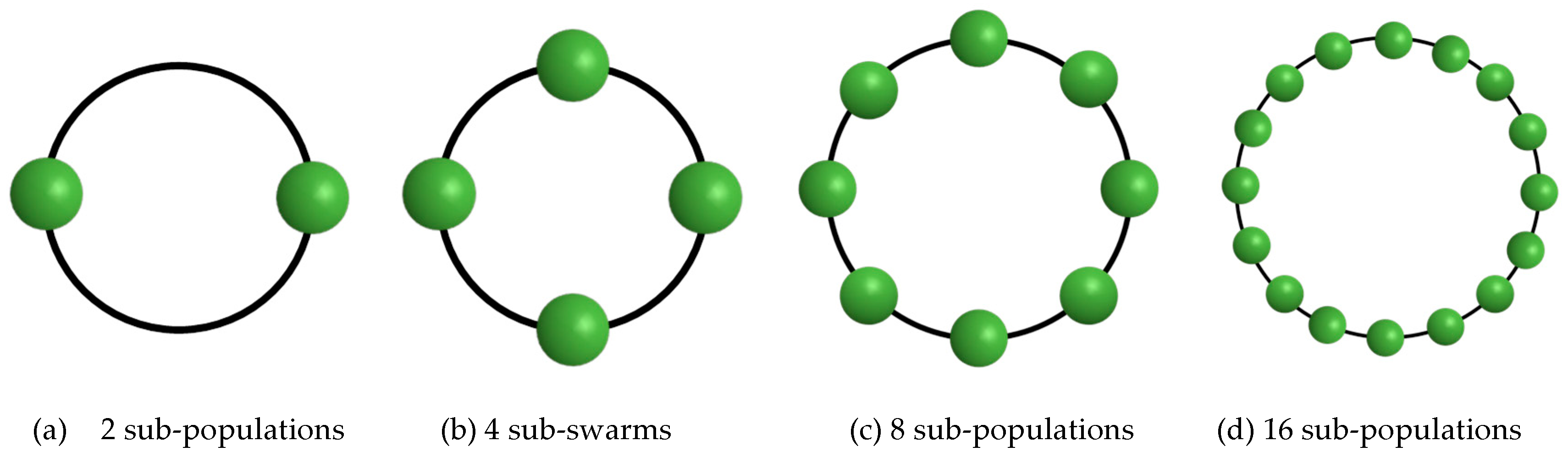
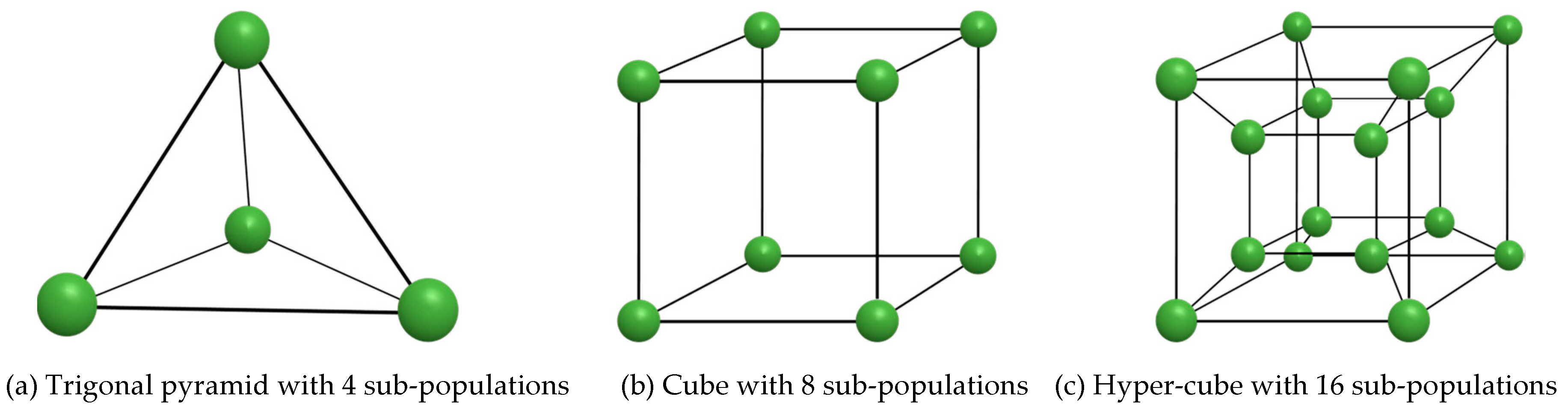
- Migration topology: topological structures of sub-populations. Ring topology with 2, 4, 8, and 16 sub-populations (see Figure 6a–d), trigonal pyramid topology with four sub-populations, a cube topology with eight sub-populations, or hyper-cube topology with 16 sub-populations (see Figure 7a–c) can be utilized.
- -
- Migration interval: how often searching individuals migrate.
- -
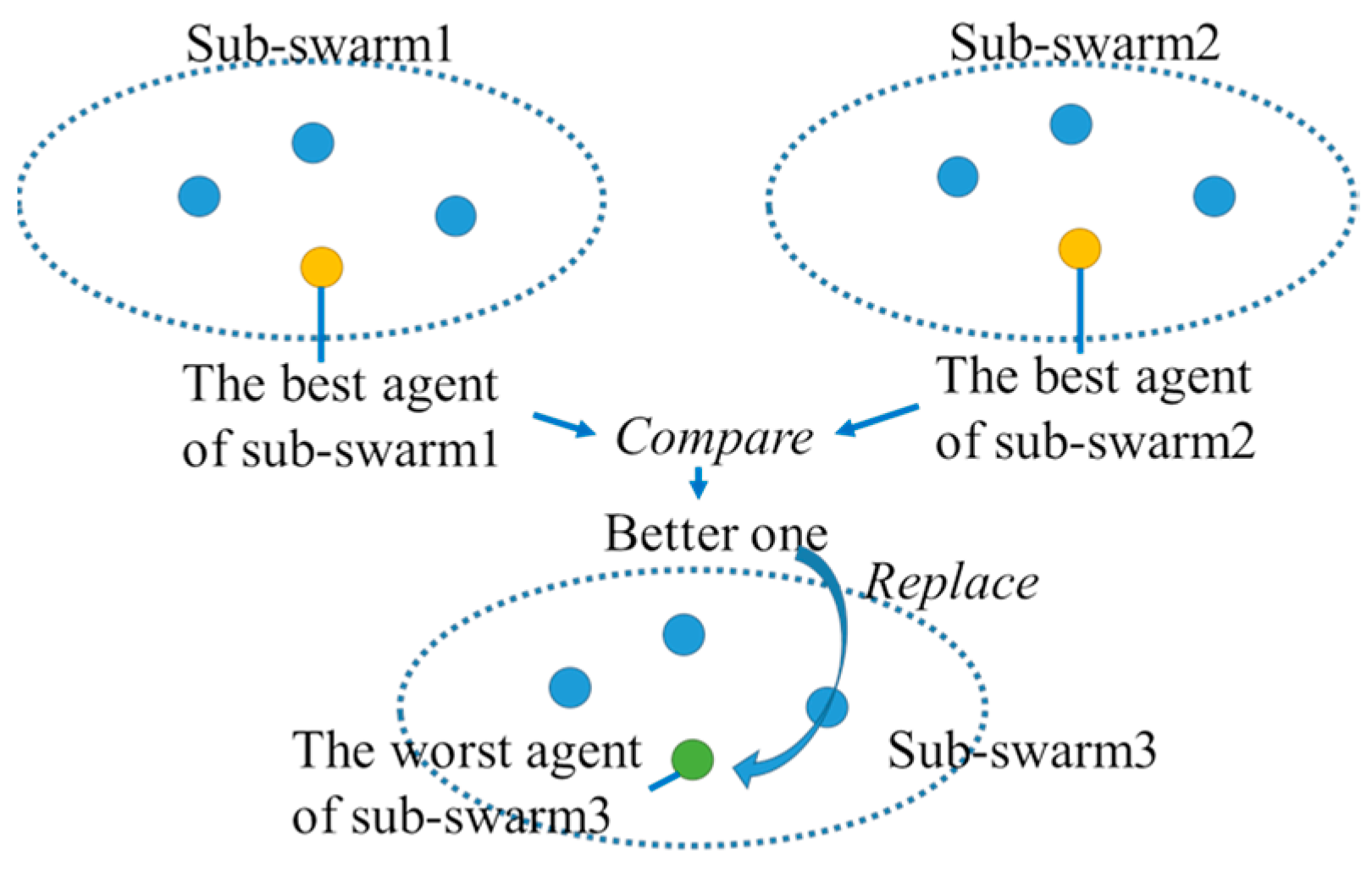
- Migration policy: the way to select searching individuals for replacement in the receiving sub-population and the way to select searching individuals for migration in the sending sub-population. The worst individual of the receiving sub-population is replaced by the best individual of the sending sub-populations (W-B) (see Figure 8) , a randomly selected individual of the receiving sub-population is replaced by the best individual of the sending sub-populations (R-B) , the best individual of the receiving sub-population is replaced by the best individual of the sending sub-populations (B-B), the worst individual of the receiving sub-population is replaced by a randomly selected individual of the sending sub-populations (W-R), a randomly selected individual of the receiving sub-population is replaced by a randomly selected individual of the sending sub-populations (R-R), the best individual of the receiving sub-population is replaced by a randomly selected individual of the sending sub-populations (B-R), the worst individual of the receiving sub-population is replaced by the worst individual of the sending sub-populations (W-W), a randomly selected individual of the receiving sub-population is replaced by the worst individual of the sending sub-populations (R-W), or the best individual of the receiving sub-population is replaced by the worst individual of the sending sub-populations (B-W), can be utilized .
4.6. Update Equations of The Proposed MP-GMBSO with Migration
- -
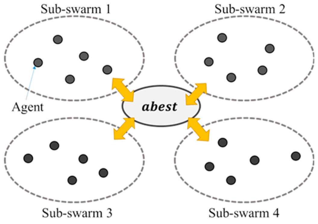
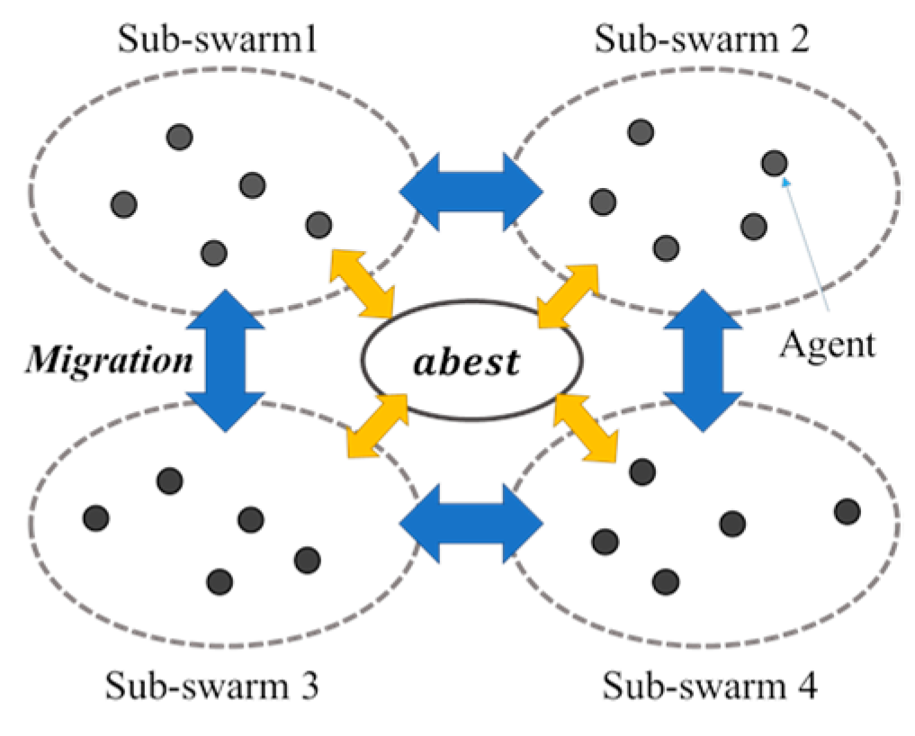
- the proposed MP-GMBSO with only migration model (see Figure 3):where is decision variable of the th individual in sub-population , and is decision variable of the best individual in sub-population .
- -
5. Total Optimization of Energy Networks in a Smart City by Multi-Population Global-Best Modified Brain Storm Optimization with Migration
5.1. Cutout Transformation Function
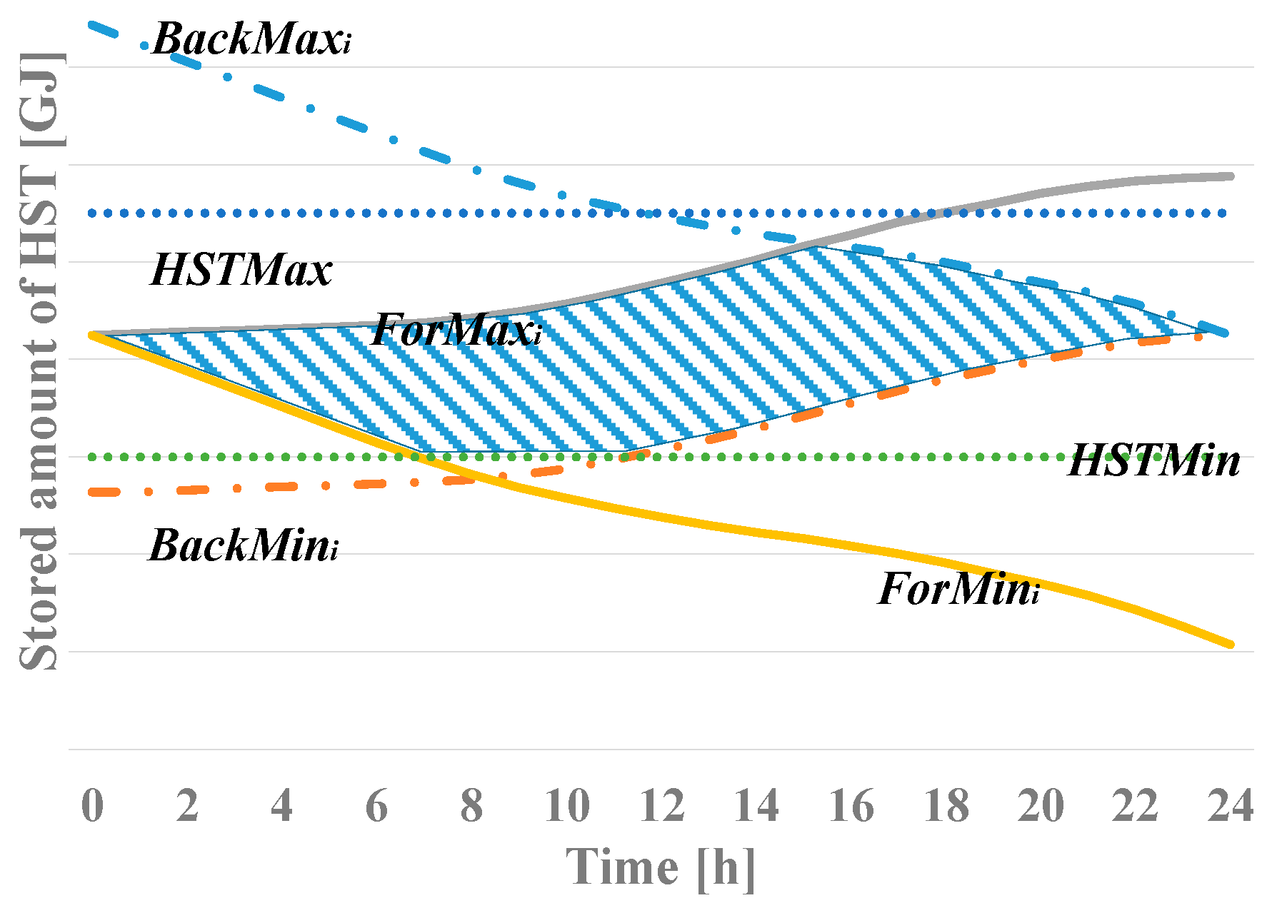
5.2. Reduction of Search Space
5.3. The Proposed Total Optimization Algorithm of Smart City by MP-GMBSO with Migration
- Step 1
- Initialization: Divide all individuals into sub-populations. Generate initial individuals at each sub-population considering the reduced search space for a smart city.
- Step 2
- Calculate the objective function at all individuals in sub-populations.
- Step 3
- Clustering:
- Step 3-1
- Generate clusters using in all sub-populations.
- Step 3-2
- Calculate objective functions of all individuals in each cluster in all sub-populations.
- Step 3-3
- Rank individuals ascending order.
- Step 3-4
- The highest rank individuals at each cluster of all sub-populations are set as cluster centers. If randomly generate a new individual and replace a cluster center with the newly generated individual.
- Step 4
- Generation of new individual: When condition (9) is satisfied, information of “gbest” is applied to using (13) or (14). New individuals are generated considering several conditions explained in 4.1.2 using Equation (15).
- Step 5
- Selection:
- Step 5-1
- The objective function values are calculated for all individuals.
- Step 5-2
- The new individual is compared with the current individual with the same individual index. Keep the better one and the individual is stored as the current individual in all sub-populations.
- Step 6
- Evaluation: Calculate objective function values of individuals in all sub-populations. The best individual is updated when the objective function value of the individual is better than the current best individual.
- Step 7
- Individuals are migrated when the current iteration number reaches the migration interval which is pre-determined.
- Step 8
- the whole procedure is stopped and go to Step 9 when the current number of iterations reaches the maximum number of iterations which is pre-determined. Otherwise, go to Step 3 and repeat the procedures.
- Step 9
- The finally obtained objective function value and the best operational values are output as a final solution.
6. Simulations
6.1. Simulation Conditions
- Case 1:
- a goal of a general smart city considering all three terms of the objective function equally,
- Case 2:
- a goal of an industrial park which usually concentrates only minimization of total energy cost
- Case 3:
- a goal of local government of a city which usually concentrates only minimization of CO2 emission.
- : 0.2, : 0.006, : 0.75, the initial weight coefficients (A, B, and C): 0.5, the number of clones: 1.
- , , , , 0.2 (for MBSO, GMBSO), , (for GBSO and GMBSO).
- -
- The initial weight coefficients of each term (D) is set to 0.5,
- -
- The number of sub-populations (NumSubPop): 2, 4, 8, and 16,
- -
- The total number of individuals (NumInd): 1280 (640 individuals/sub-population for 2 sub-populations, 320 individuals/sub-population for 4 sub-populations, 160 individuals/sub-population for 8 sub-populations, and 80 individuals/sub-population for 16 sub-populations), 640 (320 individuals/sub-population for 2 sub-populations, 160 individuals/sub-population for 4 sub-populations, 80 individuals/sub-population for 8 sub-populations, and 40 individuals/sub-population for 16 sub-populations), 320 (160 individuals/sub-population for 2 sub-populations, 80 individuals/sub-population for 4 sub-populations, 40 individuals/sub-population for 8 sub-populations, and 20 individuals/sub-population for 16 sub-populations), 160 (80 individuals/sub-population for 2 sub-populations, 40 individuals/sub-population for 4 sub-populations, 20 individuals/sub-population for 8 sub-populations, and 10 individuals/sub-population for 16 sub-populations), and 80 (40 individuals/sub-population for 2 sub-populations, 20 individuals/sub-population for 4 sub-populations, 10 individuals/sub-population for 8 sub-populations).
- -
- -
- Migration interval: 10 to 100 in 10 increments,
- -
- Migration policy: W-B, R-B, B-B, W-R, R-R, B-R, W-W, R-W, B-W.
- -
- The number of trials: 50
- -
- The maximum iteration number for BSO, GBSO, MBSO, and GMBSO based methods: 2000
- -
- The maximum iteration number for DEEPSO based method is set to 1000
6.2. Simulation Results
7. Conclusions
Author Contributions
Funding
Conflicts of Interest
References
- Jaber, S.A.A. The MASDAR Initiative. In Proceedings of the First International Energy 2030 Conference, Abu Dhabi, UAE, 1–2 November 2006; pp. 36–37. [Google Scholar]
- Ministry of Economy, Trade, and Industry of Japan, Smart Community. Available online: http://www.meti.go.jp/english/policy/energy_environment/smart_community/ (accessed on 12 December 2018).
- Reconstruction Agency. Available online: http://www.reconstruction.go.jp/english/ (accessed on 20 December 2018).
- Henze, M. (Ed.) Activated Sludge Models ASM1, ASM2, ASM2d and ASM3; Scientific and Technical Report No. 9; IWA Publishing: London, UK, 2000. [Google Scholar]
- Makino, Y.; Fujita, H.; Lim, Y.; Tan, Y. Development of a Smart Community Simulator with Individual Emulation Modules for Community Facilities and Houses. In Proceedings of the IEEE 4th Global Conference on Consumer Electronics (GCCE), Osaka, Japan, 27–30 October 2015. [Google Scholar]
- Marckle, G.; Savic, D.A.; Walters, G.A. Application of Genetic Algorithms to Pump Scheduling for Water Supply. In Proceedings of the First International Conference on Genetic Algorithms in Engineering Systems: Innovations and Applications, Sheffield, UK, 12–14 September 1995. [Google Scholar]
- Suzuki, R.; Okamoto, T. An Optimization Benchmark Problem for Operational Planning of an Energy Plant. In Proceedings of the Electronics, Information, and Systems Society Meeting of IEEJ, TC7-2, Aomori, Japan, 5–7 September 2012. (In Japanese). [Google Scholar]
- Yasuda, K. Definition and Modelling of Smart Community. In Proceedings of the IEEJ National Conference, 1-H1-2, Tokyo, Japan, 24–25 March 2015. (In Japanese). [Google Scholar]
- Yamaguchi, N.; Ogata, T.; Ogita, Y.; Asanuma, S. Modelling Energy Supply Systems in Smart Community. In Proceedings of the Annual Meeting of the IEEJ, 1-H1-3, Tokyo, Japan, 24–25 March 2015. (In Japanese). [Google Scholar]
- Matsui, T.; Kosaka, T.; Komaki, D.; Yamaguchi, N.; Fukuyama, Y. Energy Consumption Models in Smart Community. In Proceedings of the Annual Meeting of the IEEJ, 1-H1-4, Tokyo, Japan, 24–25 March 2015. (In Japanese). [Google Scholar]
- Sato, M.; Fukuyama, Y. Total Optimization of Smart Community by Particle Swarm Optimization Considering Reduction of Search Space. In Proceedings of the 2016 IEEE International Conference on Power System Technology (POWERCON), Wollongong, NSW, Australia, 28 September–1 October 2016. [Google Scholar]
- Sato, M.; Fukuyama, Y. Total Optimization of Smart Community by Differential Evolution Considering Reduction of Search Space. In Proceedings of the IEEE TENCON 2016, Singapore, 22–25 November 2016. [Google Scholar]
- Sato, M.; Fukuyama, Y. Total Optimization of Smart Community by Differential Evolutionary Particle Swarm Optimization. In Proceedings of the IFAC World Congress 2017, Toulouse, France, 9–14 July 2017. [Google Scholar]
- Sato, M.; Fukuyama, Y. Total Optimization of Smart Community by Brain Storm Optimization. In Proceedings of the SICE Annual Conference 2018, Nara, Japan, 11–14 September 2018. [Google Scholar]
- Sato, M.; Fukuyama, Y. Total Optimization of Smart Community by Modified Brain Storm Optimization. In Proceedings of the 10th Symposium on Control of Power and Energy Systems (IFAC CPES2018), Tokyo, Japan, 4–6 September 2018. [Google Scholar]
- Sato, M.; Fukuyama, Y. Total Optimization of Smart Community by Global-best Brain Storm Optimization. In Proceedings of the GECCO 2018, Kyoto, Japan, 15–19 July 2018. [Google Scholar]
- Sato, M.; Fukuyama, Y.; Iizaka, T.; Matsui, T. Total Optimization of Smart Community by Global-best Modified Brain Storm Optimization. In Proceedings of the 11th International Joint Conference on Computational Intelligence (IJCCI 2018), Seville, Spain, 18–20 September 2018. [Google Scholar]
- Fukuyama, Y.; Chiang, H.D. A Parallel Genetic Algorithm for Generation Planning. IEEE Trans. Power Syst. 1996, 11, 955–961. [Google Scholar] [CrossRef]
- Lou, S.-H.; Wu, Y.-W.; Xiong, X.-Y.; Tu, G.-Y. A Parallel PSO Approach to Multi-Objective Reactive Power Optimization with Static Voltages Stability Consideration. In Proceedings of the IEEE Transmission and Distribution Conference and Exhibition, Dallas, TX, USA, 21–24 May 2006. [Google Scholar]
- Wang, D.; Wu, C.H.; Ip, A.; Wang, D.; Yan, Y. Parallel Multi-Population Particle Swarm Optimization Algorithm for the Uncapacitated Facility Location Problem using OpenMP. In Proceedings of the IEEE Congress on Evolutionary Computation (CEC) Conference, Hong Kong, China, 1–6 June 2008. [Google Scholar]
- Lorion, Y.; Bogon, T.; Timm, I.J.; Drobnik, O. An Agent Based Parallel Particle Swarm Optimization-APPSO. In Proceedings of the Swarm Intelligence Symposium (SIS), Nashville, TN, USA, 30 March–2 April 2009; pp. 52–59. [Google Scholar]
- Yazawa, K.; Tamura, K.; Yasuda, K.; Motoki, M.; Ishigame, A. Cluster-Structured Particle Swarm Optimization with Interaction and Adaptation. Electron. Commun. Jpn. 2011, 94, 9–17. [Google Scholar] [CrossRef]
- Lopes, R.A.; Pedrosa, R.C.; Campelo, F.; Guimaraes, G. A Multi-Agent Approach to the Adaptation of migration Topology in Island Model Evolutionary Algorithms. In Proceedings of the 2012 Brazilian Symposium on Neural Networks (SBRN), Curitiba, Brazil, 20–25 October 2012. [Google Scholar]
- Tang, J.; Lim, M.H.; Ong, Y.S.; Er, M.J. Study of migration topology in island model parallel hybrid-GA for large scale quadratic assignment problems. In Proceedings of the Eighth International Conference on Control, Automation, Robotics and Vision, Special Session on Computational Intelligence on the Grid, Kunming, China, 6–9 December 2014. [Google Scholar]
- Singh, H.; Srivastava, L. Optimal VAR control for Real Power Loss Minimization Voltage Stability Improvement using Hybrid Multi-Swarm PSO. In Proceedings of the International Conference on Circuit, Power and Computing Technologies (ICCPCT), Nagercoil, India, 18–19 March 2016. [Google Scholar]
- Sato, M.; Fukuyama, Y. Total Optimization of Smart Community by Multi-Swarm Differential Evolutionary Particle Swarm Optimization. In Proceedings of the IEEE Symposium Series on Computational Intelligence 2017 (SSCI 2017), Honolulu, HI, USA, 27 November–1 December 2017. [Google Scholar]
- Sato, M.; Fukuyama, Y.; Iizaka, T.; Matsui, T. Total Optimization of Energy Networks in a Smart City by Multi-Swarm Differential Evolutionary Particle Swarm Optimization. IEEE Trans. Sustain. Energy. [CrossRef]
- Shi, Y. Brain Storm Optimization Algorithm. In Proceedings of the International Conference in Swarm Intelligence, Chongqing, China, 12–15 June 2011; Lecture Notes in Computer Science. Volume 6728, pp. 295–303. [Google Scholar]
- Zhan, Z.; Zhang, J.; Shi, Y.; Liu, H. A Modified Brain Storm Optimization. In Proceedings of the 2012 IEEE Congress on Evolutionary Computation, Brisbane, Australia, 10–15 June 2012. [Google Scholar]
- El-Adb, M. Global-best brain storm optimization algorithm. Swarm Evol. Comput. 2017, 37, 27–44. [Google Scholar]
- Sato, M.; Fukuyama, Y.; Iizaka, T.; Matsui, T. Total Optimization of Smart City by Multi-population Global-best Modified Brain Storm Optimization. Proceedings of Joint 10th International Conference on Soft Computing and Intelligent Systems and 19th International Symposium on Advanced Intelligent Systems in conjunction with Intelligent Systems Workshop 2018 (SCIS&ISIS 2018), Toyama, Japan, 5–8 December 2018. [Google Scholar]
- Kanno, T.; Matsui, T.; Fukuyama, Y. Various Scenarios and Simulation Examples Using Smart Community Models. In Proceedings of the Annual Meeting of the IEEJ, Tokyo, Japan, 24–25 March 2015. (In Japanese). [Google Scholar]


| Sector | Decision Variables |
|---|---|
| Industrial sector | Output of electric power of a gas turbine generator (GTG), Heat output of turbo refrigerators (TRs), Heat output of stream refrigerators (SRs), Charged or discharged electric power of a storage battery (SB) |
| Building sector | Output of electric power of a GTG, Heat output of TRs, Heat output of SRs |
| Residential sector | Heat output of SRs, Output of electric power of a fuel cell, Heat output of a heat pump water heater, Charged or discharged electric power of a SB |
| Railroad sector | The number of passengers/h, Average of journey distance by one passenger/h, The number of operated trains/h, The numbers of passenger cars/set, Average of journey distance by one train/h, Average of speed/h, The number of passengers/car |
| Drinking water treatment plant sector | Inflow from river, Inflow of water into a service reservoir, Output of electric power output of a co-generator (CoGen), Charged or discharged electric power of a SB |
| Wastewater treatment plant sector | Input of Pumped wastewater, Output of electric power of a CoGen, Charged or discharged electric power of a SB |
| Case | Mean | Min. | Max. | Std. | |
|---|---|---|---|---|---|
| 1 | DEEPSO | 100.00 | 98.75 | 101.63 | 0.57 |
| BSO | 97.13 | 96.46 | 97.96 | 0.30 | |
| GBSO | 95.94 | 95.55 | 97.03 | 0.26 | |
| MBSO | 97.20 | 96.75 | 97.66 | 0.20 | |
| GMBSO | 95.06 | 94.90 | 95.29 | 0.09 | |
| 2 | DEEPSO | 100.00 | 99.53 | 100.58 | 0.20 |
| BSO | 99.28 | 98.98 | 99.60 | 0.14 | |
| GBSO | 98.29 | 98.22 | 98.42 | 0.04 | |
| MBSO | 99.38 | 99.15 | 99.50 | 0.06 | |
| GMBSO | 98.26 | 98.17 | 98.36 | 0.04 | |
| 3 | DEEPSO | 100.00 | 99.44 | 100.88 | 0.32 |
| BSO | 99.64 | 99.38 | 99.87 | 0.09 | |
| GBSO | 99.36 | 99.12 | 99.53 | 0.10 | |
| MBSO | 98.37 | 98.30 | 98.46 | 0.04 | |
| GMBSO | 98.10 | 98.05 | 98.16 | 0.03 |
| DEEPSO | BSO | GBSO | MBSO | GMBSO | p-value | |
|---|---|---|---|---|---|---|
| Case 1 | 5 | 3.34 | 2 | 3.66 | 1 | |
| Case 2 | 5 | 3.22 | 1.6 | 3.78 | 1.4 | |
| Case 3 | 4.92 | 4.08 | 3 | 2 | 1 |
| Model | Mig. Policy | # of sub-pop. | Ring | Trigonal Pyramid/Cube/Hyper-Cube | ||||||||
|---|---|---|---|---|---|---|---|---|---|---|---|---|
| Mean | Min. | Max. | Std. | Ave. Rank | Mean | Min. | Max. | Std. | Ave. Rank | |||
| - | - | 1 | 100.00 | 99.90 | 100.17 | 0.06 | 18.82 | - | - | - | - | - |
| Abest | - | 2 | 99.94 | 99.82 | 100.06 | 0.05 | 17.44 | - | - | - | - | - |
| 4 | 99.89 | 99.79 | 99.99 | 0.04 | 16.22 | - | - | - | - | - | ||
| 8 | 99.80 | 99.73 | 99.89 | 0.03 | 11.66 | - | - | - | - | - | ||
| 16 | 99.71 | 99.59 | 99.83 | 0.04 | 5.64 | - | - | - | - | - | ||
| Abest & Mig. | W-B | 2 | 99.85 | 99.73 | 99.92 | 0.05 | 14.28 | - | - | - | - | - |
| 4 | 99.79 | 99.67 | 99.87 | 0.05 | 10.52 | 99.80 | 99.71 | 99.91 | 0.05 | 11.02 | ||
| 8 | 99.73 | 99.62 | 99.86 | 0.05 | 6.76 | 99.75 | 99.53 | 99.86 | 0.06 | 8.3 | ||
| 16 | 99.67 | 99.5 | 99.83 | 0.08 | 4.52 | 99.73 | 99.53 | 99.87 | 0.08 | 7.04 | ||
| Mig. | W-B | 2 | 99.86 | 99.78 | 99.97 | 0.04 | 15.46 | - | - | - | - | - |
| 4 | 99.78 | 99.69 | 99.89 | 0.05 | 9.94 | 99.79 | 99.71 | 99.87 | 0.04 | 11.18 | ||
| 8 | 99.72 | 99.59 | 99.82 | 0.06 | 6.18 | 99.73 | 99.6 | 99.89 | 0.06 | 6.8 | ||
| 16 | 99.63 | 99.45 | 99.82 | 0.09 | 3.14 | 99.68 | 99.52 | 99.91 | 0.08 | 5.08 | ||
| p-value | ||||||||||||
| Model | Mig. Policy | # of sub-pop. | Ring | ||||
|---|---|---|---|---|---|---|---|
| Mean | Min. | Max. | Std. | Ave. Rank | |||
| - | - | 1 | 100.00 | 99.90 | 100.17 | 0.06 | 4 |
| Abest | - | 16 | 99.71 | 99.59 | 99.83 | 0.04 | 2.4 |
| Abest & Mig. | W-B | 16 | 99.67 | 99.5 | 99.83 | 0.08 | 2.02 |
| Mig. | W-B | 16 | 99.63 | 99.45 | 99.82 | 0.09 | 1.58 |
| p-value | |||||||
| Policy | NSP | Ring | Ave. Rank | Cube/Trigonal Pyramid/Hypercube | Ave. Rank | ||||||
|---|---|---|---|---|---|---|---|---|---|---|---|
| Mean | Min. | Max. | Std. | Mean | Min. | Max. | Std. | ||||
| - | 1 | 100 | 99.9 | 100.17 | 0.06 | 38.78 | - | - | - | - | - |
| B-B | 2 | 99.93 | 99.82 | 100.08 | 0.05 | 33.48 | - | - | - | - | - |
| 4 | 99.89 | 99.75 | 100.05 | 0.05 | 28.48 | 99.89 | 99.8 | 100 | 0.05 | 27.94 | |
| 8 | 99.82 | 99.72 | 99.88 | 0.04 | 19.14 | 99.81 | 99.72 | 99.95 | 0.05 | 18.78 | |
| 16 | 99.71 | 99.61 | 99.85 | 0.06 | 8.2 | 99.71 | 99.61 | 99.79 | 0.04 | 7.88 | |
| W-W | 2 | 48.12 | - | - | - | - | - | ||||
| 4 | 48.82 | 49.46 | |||||||||
| 8 | 51.2 | 50.32 | |||||||||
| 16 | 101.55 | 52.24 | 102.12 | 52.52 | |||||||
| W-B | 2 | 99.86 | 99.78 | 99.97 | 0.04 | 25.6 | - | - | - | - | |
| 4 | 99.78 | 99.69 | 99.89 | 0.05 | 14.96 | 99.79 | 99.71 | 99.87 | 0.04 | 16.62 | |
| 8 | 99.72 | 99.59 | 99.82 | 0.06 | 8.98 | 99.73 | 99.6 | 99.89 | 0.06 | 10.42 | |
| 16 | 99.63 | 99.45 | 99.82 | 0.09 | 4.54 | 99.68 | 99.52 | 99.91 | 0.08 | 7.54 | |
| B-W | 2 | 54.6 | - | - | - | - | - | ||||
| 4 | 56.8 | 56.98 | |||||||||
| 8 | 59.36 | 57.22 | |||||||||
| 16 | 61.16 | 60.44 | |||||||||
| B-R | 2 | 99.92 | 99.81 | 99.99 | 0.04 | 31.46 | - | - | - | - | - |
| 4 | 100.14 | 100.02 | 100.25 | 0.05 | 42.56 | 100.11 | 100.02 | 100.22 | 0.05 | 42.26 | |
| 8 | 99.95 | 99.84 | 100.05 | 0.06 | 34.72 | 99.95 | 99.83 | 100.06 | 0.05 | 35.32 | |
| 16 | 99.92 | 99.81 | 99.99 | 0.04 | 31.46 | 99.88 | 99.79 | 99.96 | 0.04 | 27.84 | |
| R-B | 2 | 99.96 | 99.83 | 100.05 | 0.06 | 35.46 | - | - | - | - | - |
| 4 | 99.89 | 99.76 | 99.98 | 0.05 | 28.2 | 99.91 | 99.8 | 100.05 | 0.05 | 30.84 | |
| 8 | 99.82 | 99.72 | 99.92 | 0.05 | 19.16 | 99.81 | 99.69 | 99.9 | 0.04 | 18.88 | |
| 16 | 99.7 | 99.58 | 99.84 | 0.06 | 7.34 | 99.7 | 99.58 | 99.89 | 0.06 | 7.3 | |
| W-R | 2 | 99.99 | 99.87 | 100.09 | 0.06 | 38 | - | - | - | - | - |
| 4 | 99.91 | 99.83 | 100 | 0.04 | 31.04 | 99.9 | 99.75 | 99.96 | 0.04 | 29.84 | |
| 8 | 99.82 | 99.7 | 99.89 | 0.04 | 19.24 | 99.76 | 99.65 | 99.84 | 0.04 | 12.58 | |
| 16 | 99.69 | 99.61 | 99.77 | 0.03 | 6.14 | 99.64 | 99.55 | 99.77 | 0.05 | 3.74 | |
| R-W | 2 | 49.42 | - | - | - | - | - | ||||
| 4 | 51.16 | 51 | |||||||||
| 8 | 52.92 | 52.6 | |||||||||
| 16 | 58.84 | 58.78 | |||||||||
| R-R | 2 | 99.93 | 99.85 | 100.05 | 0.04 | 33.42 | - | - | - | - | 26.56 |
| 4 | 99.87 | 99.79 | 99.99 | 0.04 | 26.54 | 99.94 | 99.85 | 100.07 | 0.04 | 18.48 | |
| 8 | 99.81 | 99.74 | 99.89 | 0.03 | 18.32 | 99.81 | 99.66 | 99.93 | 0.05 | 9.4 | |
| 16 | 99.7 | 99.62 | 99.84 | 0.05 | 7.56 | 99.71 | 99.6 | 99.87 | 0.06 | 26.56 | |
| p-value | 0 | ||||||||||
| Policy | NSP | Ring | Ave. Rank | |||
|---|---|---|---|---|---|---|
| Mean | Min. | Max. | Std. | |||
| - | 1 | 100 | 99.9 | 100.17 | 0.06 | 6.9 |
| B-B | 16 | 99.71 | 99.61 | 99.85 | 0.06 | 3.42 |
| W-W | 16 | 101.55 | 8.32 | |||
| W-B | 16 | 99.63 | 99.45 | 99.82 | 0.09 | 2.16 |
| B-W | 2 | 9.58 | ||||
| B-R | 16 | 99.92 | 99.81 | 99.99 | 0.04 | 6.04 |
| R-B | 16 | 99.7 | 99.58 | 99.84 | 0.06 | 3.16 |
| W-R | 16 | 99.69 | 99.61 | 99.77 | 0.03 | 3 |
| R-W | 16 | 9.1 | ||||
| R-R | 16 | 99.7 | 99.62 | 99.84 | 0.05 | 3.32 |
| p-value | ||||||
| NI | NSP | Ring | Ave.Rank | Cube/Trigonal Pyramid/Hypercube | Ave.Rank | ||||||
|---|---|---|---|---|---|---|---|---|---|---|---|
| Mean | Min. | Max. | Std. | Mean | Min. | Max. | Std. | ||||
| 40 | 1 | 99.85 | 99.73 | 100.06 | 0.06 | 38.8 | - | - | - | - | - |
| 2 | 99.93 | 99.73 | 100.21 | 0.11 | 34.1 | - | - | - | - | - | |
| 4 | 99.78 | 39.42 | 100.03 | 99.79 | 100.33 | 0.12 | 38.8 | ||||
| 8 | 100.08 | 45.64 | 99.96 | 44.24 | |||||||
| 80 | 1 | 99.91 | 99.81 | 100.02 | 0.04 | 34.32 | - | - | - | - | - |
| 2 | 99.79 | 99.64 | 100.03 | 0.08 | 22.84 | - | - | - | - | - | |
| 4 | 99.81 | 99.63 | 100.01 | 0.09 | 24.02 | 99.86 | 99.65 | 100.09 | 0.10 | 12.1 | |
| 8 | 99.87 | 99.64 | 100.18 | 0.12 | 29.06 | 99.86 | 99.71 | 100.11 | 0.09 | 19.08 | |
| 16 | 99.72 | 99.54 | 99.89 | 0.08 | 14.72 | 99.91 | 99.70 | 100.12 | 0.10 | 31.56 | |
| 160 | 1 | 99.95 | 99.82 | 100.14 | 0.07 | 36.64 | - | - | - | - | - |
| 2 | 99.77 | 99.68 | 99.90 | 0.05 | 31.34 | - | - | - | - | - | |
| 4 | 99.77 | 99.58 | 99.99 | 0.08 | 16.42 | 99.77 | 99.61 | 100.03 | 0.08 | 15.78 | |
| 8 | 99.73 | 99.56 | 99.89 | 0.08 | 7 | 99.73 | 99.52 | 99.98 | 0.11 | 8.48 | |
| 16 | 99.57 | 99.42 | 99.86 | 0.09 | 3.64 | 99.67 | 99.53 | 99.92 | 0.09 | 7.66 | |
| 320 | 1 | 99.97 | 99.83 | 100.10 | 0.06 | 38.38 | - | - | - | - | - |
| 2 | 99.81 | 99.68 | 99.97 | 0.05 | 36.56 | - | - | - | - | - | |
| 4 | 99.77 | 99.64 | 99.88 | 0.05 | 27.64 | 99.77 | 99.64 | 99.87 | 0.05 | 27.52 | |
| 8 | 99.71 | 99.56 | 99.81 | 0.06 | 13.74 | 99.69 | 99.54 | 99.82 | 0.07 | 10.02 | |
| 16 | 99.56 | 99.41 | 99.77 | 0.09 | 2 | 99.66 | 99.51 | 99.93 | 0.09 | 4.38 | |
| 640 | 1 | 100.00 | 99.90 | 100.17 | 0.06 | 39.64 | - | - | - | - | - |
| 2 | 99.86 | 99.78 | 99.97 | 0.04 | 31.02 | - | - | - | - | - | |
| 4 | 99.78 | 99.69 | 99.89 | 0.05 | 21.46 | 99.79 | 99.71 | 99.87 | 0.04 | 23.24 | |
| 8 | 99.72 | 99.59 | 99.82 | 0.06 | 14.88 | 99.73 | 99.60 | 99.89 | 0.06 | 16.12 | |
| 16 | 99.63 | 99.45 | 99.82 | 0.09 | 8.58 | 99.68 | 99.52 | 99.91 | 0.08 | 12.16 | |
| 1280 | 1 | 100.75 | 100.59 | 100.91 | 0.07 | 44.66 | - | - | - | - | - |
| 2 | 99.88 | 99.79 | 99.96 | 0.04 | 32.34 | - | - | - | - | - | |
| 4 | 99.83 | 99.76 | 99.89 | 0.04 | 25.9 | 99.84 | 99.75 | 100.03 | 0.05 | 27.6 | |
| 8 | 99.77 | 99.66 | 99.84 | 0.04 | 18.86 | 99.77 | 99.68 | 99.88 | 0.04 | 19.7 | |
| 16 | 99.68 | 99.57 | 99.82 | 0.06 | 12.74 | 99.70 | 99.51 | 99.82 | 0.06 | 15.2 | |
| p-value | 0 | ||||||||||
| NI | NSP | Ring | Ave. Rank | |||
|---|---|---|---|---|---|---|
| Mean | Min. | Max. | Std. | |||
| 40 | 1 | 99.85 | 99.73 | 100.06 | 0.06 | 6 |
| 80 | 16 | 99.72 | 99.54 | 99.89 | 0.08 | 1.42 |
| 160 | 16 | 99.57 | 99.42 | 99.86 | 0.09 | 3.08 |
| 320 | 16 | 99.56 | 99.41 | 99.77 | 0.09 | 2.2 |
| 640 | 16 | 99.63 | 99.45 | 99.82 | 0.09 | 4.06 |
| 1280 | 16 | 99.68 | 99.57 | 99.82 | 0.06 | 6 |
| # of Pop. | 1 | 2 | 4 | 8 | 16 | |||||
|---|---|---|---|---|---|---|---|---|---|---|
| Hours | A | B | A | B | A | B | A | B | A | B |
| 1 | 6.23 | 0.90 | 0.00 | 7.14 | 6.64 | 0.36 | 6.00 | 1.27 | 7.04 | 0.21 |
| 2 | 6.28 | 0.97 | 0.00 | 7.00 | 6.56 | 0.81 | 6.32 | 0.89 | 6.56 | 0.75 |
| 3 | 6.65 | 0.64 | 6.72 | 0.47 | 6.00 | 1.20 | 7.04 | 0.23 | 6.28 | 1.02 |
| 4 | 6.00 | 1.18 | 0.00 | 7.30 | 6.14 | 1.19 | 6.30 | 0.94 | 7.06 | 0.26 |
| 5 | 7.52 | 1.82 | 8.69 | 0.57 | 7.84 | 1.47 | 9.00 | 0.22 | 6.00 | 3.23 |
| 6 | 6.77 | 2.49 | 6.00 | 3.11 | 6.68 | 2.45 | 6.73 | 2.17 | 7.99 | 1.24 |
| 7 | 7.10 | 2.02 | 7.38 | 1.52 | 6.77 | 2.13 | 8.10 | 1.04 | 8.55 | 0.61 |
| 8 | 7.37 | 1.73 | 7.13 | 2.13 | 7.66 | 1.35 | 8.86 | 0.31 | 7.40 | 1.71 |
| 9 | 10.16 | 0.91 | 9.12 | 1.91 | 9.65 | 1.38 | 9.86 | 1.25 | 10.32 | 0.87 |
| 10 | 13.65 | 1.33 | 13.52 | 1.28 | 13.22 | 1.74 | 13.89 | 1.21 | 14.94 | 0.11 |
| 11 | 16.67 | 2.03 | 15.53 | 3.25 | 17.07 | 1.79 | 18.31 | 0.64 | 17.02 | 2.06 |
| 12 | 20.00 | 4.75 | 17.79 | 7.22 | 17.73 | 7.24 | 15.46 | 9.41 | 19.39 | 5.45 |
| 13 | 16.65 | 0.95 | 17.09 | 0.67 | 16.82 | 0.97 | 17.70 | 0.15 | 16.79 | 1.11 |
| 14 | 19.29 | 2.84 | 18.92 | 3.15 | 18.81 | 3.38 | 19.53 | 2.56 | 19.49 | 2.72 |
| 15 | 20.00 | 3.18 | 20.00 | 3.42 | 18.98 | 4.24 | 19.30 | 3.86 | 19.34 | 3.81 |
| 16 | 15.72 | 5.43 | 19.24 | 1.94 | 18.69 | 2.67 | 18.07 | 3.25 | 19.47 | 1.83 |
| 17 | 20.00 | 3.05 | 19.24 | 3.78 | 19.92 | 2.87 | 19.56 | 3.32 | 18.31 | 4.65 |
| 18 | 20.00 | 2.05 | 16.25 | 5.79 | 18.79 | 3.39 | 18.73 | 3.40 | 20.00 | 2.21 |
| 19 | 18.79 | 4.24 | 18.98 | 4.08 | 16.80 | 6.41 | 19.87 | 3.21 | 19.98 | 3.23 |
| 20 | 12.76 | 8.43 | 20.00 | 1.13 | 20.00 | 1.00 | 20.00 | 1.23 | 19.51 | 1.57 |
| 21 | 16.91 | 0.41 | 15.54 | 1.63 | 16.52 | 0.64 | 17.33 | 0.03 | 15.71 | 1.36 |
| 22 | 9.20 | 3.04 | 10.55 | 1.88 | 11.39 | 0.90 | 11.75 | 0.53 | 10.96 | 1.22 |
| 23 | 11.35 | 1.56 | 11.83 | 1.22 | 11.45 | 1.51 | 12.51 | 0.34 | 12.32 | 0.63 |
| 24 | 8.00 | 2.40 | 7.27 | 2.90 | 10.01 | 0.24 | 9.00 | 1.34 | 9.27 | 1.18 |
| Total | 237.18 | 44.39 | 238.90 | 43.27 | 242.06 | 39.96 | 248.23 | 34.35 | 248.64 | 33.92 |
© 2019 by the authors. Licensee MDPI, Basel, Switzerland. This article is an open access article distributed under the terms and conditions of the Creative Commons Attribution (CC BY) license (http://creativecommons.org/licenses/by/4.0/).
Share and Cite
Sato, M.; Fukuyama, Y.; Iizaka, T.; Matsui, T. Total Optimization of Energy Networks in a Smart City by Multi-Population Global-Best Modified Brain Storm Optimization with Migration. Algorithms 2019, 12, 15. https://doi.org/10.3390/a12010015
Sato M, Fukuyama Y, Iizaka T, Matsui T. Total Optimization of Energy Networks in a Smart City by Multi-Population Global-Best Modified Brain Storm Optimization with Migration. Algorithms. 2019; 12(1):15. https://doi.org/10.3390/a12010015
Chicago/Turabian StyleSato, Mayuko, Yoshikazu Fukuyama, Tatsuya Iizaka, and Tetsuro Matsui. 2019. "Total Optimization of Energy Networks in a Smart City by Multi-Population Global-Best Modified Brain Storm Optimization with Migration" Algorithms 12, no. 1: 15. https://doi.org/10.3390/a12010015
APA StyleSato, M., Fukuyama, Y., Iizaka, T., & Matsui, T. (2019). Total Optimization of Energy Networks in a Smart City by Multi-Population Global-Best Modified Brain Storm Optimization with Migration. Algorithms, 12(1), 15. https://doi.org/10.3390/a12010015