Abstract
This paper proposes total optimization of energy networks in a smart city by multi-population global-best modified brain storm optimization (MP-GMBSO). Many countries have conducted smart city demonstration projects for reduction of total energies and CO2 emission. The energy and environmental problem of smart city can be formulated as a mixed integer nonlinear programming (MINLP) problem. Therefore, evolutionary computation methods including variations of recently developed Brain Storm Optimization (BSO) such as Global-best BSO (GBSO), Modified BSO (MBSO), and Global-best Modified BSO (GMBSO) have been adopted to the problem. However, there is still room for improvement of quality of solution. Evolutionary computation methods with multi-population have been applied to various problems and verified to improve quality of solution. Therefore, the approach can be expected to improve quality of solution. The proposed MS-GMBSO utilizes only migration for multi-population models instead of abest which is the best individual among all sub-populations so far and both migration and abest. Various multi-population models, migration policies, the number of sub-populations, and migration topologies are also investigated. It is verified that the proposed MP-GMBSO based method with migration using ring topology, the W-B policy, and 320 individuals is the most effective among all of multi-population parameters.
1. Introduction
In various environmental problems, global warming is a serious problem all over the world. It is considered that an increase of greenhouse gas causes global warming. Hence, many countries have conducted smart city demonstration projects for reduction of total consumption energies and CO2 emission [1,2]. Smart city is an eco-city which can realize low carbon emission and energy consumption by Internet of Things (IoT), renewable energies, storage batteries, and so on. For example, in Japan, after the Great East Japan Earthquake, introduction of the smart city was investigated, especially in Tohoku area [3].
Basically, it is difficult to evaluate the actual CO2 emission reduction in the actual smart city. Therefore, a smart city model including various sector models should be utilized for the evaluation. Static models which can treat various energy balances and dynamic models which can treat dynamic behaviors have been developed separately in each sector [4,5,6,7]. However, a smart city model, which can calculate various environmental and energy loads among all sectors considering environmental and energy flow among various sectors, had not been developed. Considering these backgrounds, a smart city model was developed in order to evaluate energy costs and CO2 emission of the whole smart city considering environmental and energy flow among various sectors in Japan [8,9,10].
Using the smart city model, the authors have proposed total optimization of energy network in a whole smart city for minimization of energy costs, electric power loads at peak load hours, and CO2 emission by Particle Swarm Optimization (PSO) [11], Differential Evolution (DE) [12], Differential Evolutionary PSO (DEEPSO) [13], BSO [14], MBSO [15], GBSO [16], and GMBSO [17]. In addition, considering energy facility characteristics, energy load characteristics, cost characteristics, and continuity of weekday operation of various energy facilities, the authors have proposed reduction methods of search space in order to solve the problem effectively [11,12]. Therefore, GMBSO considering the reduction of search space can obtain the highest quality solution so far [17]. However, there is still room for improvement of quality of solution.
Multi-population based evolutionary computation methods have been verified to improve quality of solution [18,19,20,21,22,23,24,25,26]. Using the methods, one population with numbers of individuals is divided into several sub-populations with small numbers of individuals. Individuals at each sub-population perform solution search separately. Interaction models of multi-population can be divided into three groups: the migration model [18,19,21,23,24,25], the abest model [20,22], in which abest is the best searching point so far among all of sub-populations, and a model using both migration and abest. To the best of the authors' knowledge, since a model using both migration and abest has not been proposed, the authors propose the model [26]. However, the most suitable model has to be investigated for each evolutionary computation method.
Considering these backgrounds, this paper proposes total optimization of energy networks in a smart city by MP-GMBSO with only migration. MP-GMBSO with migration is newly proposed in order to realize improvement of quality of solution. The proposed MP-GMBSO with migration-based method is applied to a model of mid-sized city such as Toyama city. The results of the proposed method are compared with those of the GMBSO based method with a single population, and the MP-GMBSO based methods with only abest, and with both migration and abest model. Various numbers of sub-populations, various topologies (trigonal pyramid with four sub-populations, cube with eight sub-populations, hyper-cube with 16 sub-populations, and ring with 2, 4, 8, 16 sub-populations), various policies, various interaction models (only using migration, only using abest, and using both migration and abest), and various numbers of individuals have been investigated in simulation results.
The following gives a summary of the paper contributions:
- -
- A proposal of a new evolutionary computation method, namely MP-GMBSO with migration, in order to realize improvement of quality of solution,
- -
- An application of MP-GMBSO with migration-based method to total optimization of energy networks in a smart city,
- -
- Verification of efficacy of the conventional GMBSO based method for total optimization of smart city by comparing with the conventional DEEPSO, BSO, MBSO, and GBSO based methods,
- -
- Verification of efficacy of the proposed MP-GMBSO based method with migration for total optimization of smart city by comparing with the original GMBSO (GMBSO with one population) based method, and the MP-GMBSO based methods with various interaction model (only using migration, only using abest, and using both migration and abest), various policies, various topologies, various numbers of individuals, and various numbers of sub-populations,
- -
- It is verified that quality of solution is the most improved by the proposed MP-GMBSO with migration-based method using the ring topology with 16 sub-populations and 320 individuals, and the W-B policy (the worst individual of a sub-population is substituted by the best individual of other sub-populations) among all of multi-population parameters.
The rest of the paper is organized as follows. Section 2 explains a concept of the smart city model. Section 3 introduces problem formulation. Section 4 explains the details of the conventional BSO, MBSO, GBSO, and GMBSO. The proposed MP-GMBSO is also explained as well. Section 5 shows the proposed MP-GMBSO based total optimization method for energy networks in a smart city. Section 6 compares the conventional GMBSO based method with the conventional DEEPSO, BSO, MBSO, and GBSO based methods. It also presents a comparison of the proposed MP-GMBSO with migration-based method with the original GMBSO with a single population, MP-GMBSO with only abest model, and MP-GMBSO with both migration and abest model, and investigation of various migration topologies, migration policies, the number of sub-populations, and the number of individuals. Finally, Section 7 concludes the paper.
2. Smart City Model
2.1. A Summary of the Whole Smart City Model
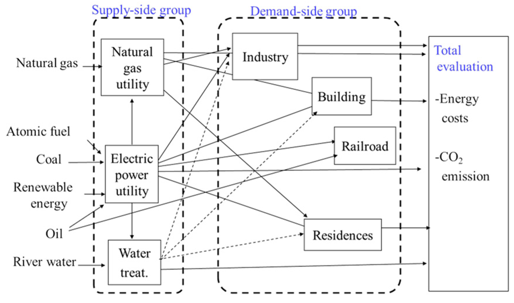
The smart city model has been developed for quantitative evaluation of a smart city. CO2 emission or energy costs of whole smart city can be quantitatively calculated by the model. Various sectors are included in the model (see Figure 1). The model deals with energy supply-side and demand-side groups. Natural gas and electric power utilities, and drinking water and wastewater treatment plant sectors are categorized into the energy supply-side group. The other sectors are categorized into the demand-side group [8,27].
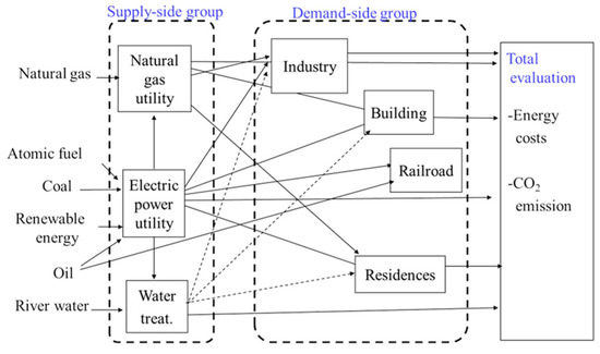
Figure 1.
Configuration of a smart city model (© 2018 IEEE [27]).
2.2. Sector Models in the Supply-Side Group
The group interactively supply energies (natural gas, electric power, and drinking water). Namely, supplied energies by supply-side sectors and energy loads of demand-side sectors should be the same. The details are shown in [9,27].
2.3. Sector Models in the Demand-Side Group
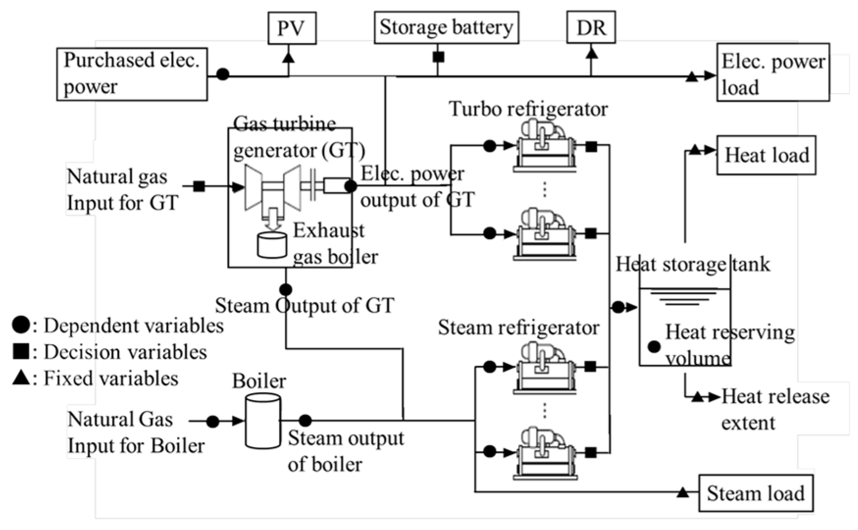
Various energy supply facilities inside each sector are modeled. Various energy loads such as electric power, hot and cold heat, and steam loads are also dealt with. The energy supply facilities supply tertiary energies to the various energy loads when operations of facilities are decided. Hence, required secondary energies are calculated, and the amount is supplied from the energy supply group when various hourly energy loads of one day (24 points) are obtained and operations of facilities (decision variables) are determined. Figure 2 shows an industrial model as an example. The details are shown in [10,27].
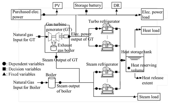
Figure 2.
A configuration of an industrial model (© 2018 IEEE [27]).
3. Problem Formulation of Total Optimization of Energy Networks in a Smart City
This paper considers smart cities such as industrial parks and local governments of cities aiming at minimization of energy cost, actual electric power at high load hours, and CO2 emission. Purchase costs of various fuels by electric power and gas companies from resource companies are not included in the problem.
3.1. Decision Variables
Decision variables in considered sectors are shown in Table 1. Each decision variable has to consider 24 hourly decision variables per day. Therefore, when the number of each facility at each sector is set to 1, the total number of decision variables can be 816. Hence, the problem can be considered as one of the large-scale optimization problems.

Table 1.
Decision variables in various sectors.
3.2. Objective Function
The objective function of the smart city problem considers three terms. The function considers minimization of energy costs of whole smart city as the first term. Actual electric power at high load hours are minimized by the second term of the function. The function also considers minimization of CO2 emission in the whole city as the third term. The functions are shown in the following Equation (1):
where is the number of sectors except electric power and natural gas utilities, is the number of hours per day (=24), is natural gas purchase at hour of sector , is a natural gas purchase unit cost at hour of sector , is electric power purchase at hour of sector , is an electric power purchase unit cost at hour of of sector , is an actual electric power load at hour of sector , is the start hour of peak load hours of actual electric power loads, the end hour of peak load hours of actual electric power loads, is a coefficient between the purchased natural gas and CO2 emission, is a coefficient between purchased electric power and CO2 emission, and , , and are weighting coefficients ().
Authors include one of a member of a smart city model committee in IEE of Japan. In the committee, a scope of a smart city has been discussed in order to consider a closed community such as industrial parks and local governments. In such a case, purchase costs of various fuels by electric power and gas companies from resource companies are not out of the scope of the city and we follow the scope in (1). After decision variables are calculated, the amounts of natural gas and electric power purchase are calculated as dependent variables. Hence, when the dependent variables violate limits of the constraints, penalty function values are calculated and they are added to the objective function values.
3.3. Constraints
- (1)
- Energy balances: Electric power, hot and cold heat, and steam energy balances are considered. These energy balances are expressed using the following equation:where is a balance equation of energy in sector , is a startup or shutdown status of a facility for decision variable , and is an input or output real value of a facility for decision variable , is the number of energies in sector , and is the number of decision variables.
- (2)
- Facility characteristics: Efficiency functions of facilities, and upper and lower bounds of various facilities in each sector can be expressed using the following equation:where is an efficiency function of facility, or upper and lower bounds of facility of sector , and is the number of facilities in sector .Efficiency of facility should be sometimes expressed with nonlinear functions. Hence, the problem is considered as one of mixed-integer nonlinear optimization problems (MINLPs) and evolutionary computation methods should be utilized in order to treat the problem.
4. The Proposed Multi-Population Global-Best Modified Brain Storm Optimization with Migration
MP-GMBSO is based on GMBSO which has been proposed using MBSO and GBSO [17]. Since MP-GMBSO is based on BSO variations, this section summarizes BSO, MBSO, GBSO and GMBSO.
4.1. Overview of BSO
BSO has developed by Shi in 2011 [28]. The BSO’s main procedure is shown below.
- Step 1
- Initialization: Randomly generate individuals and calculate the objective function values of individuals.
- Step 2
- Clustering: The k-means method is applied to divide individuals into clusters.
- Step 3
- Generation of New individual: One or two clusters are randomly selected, and new individuals are generated.
- Step 4
- Selection of individuals: Individuals which are newly generated are compared with the current individuals which have the same individual indices of the newly generated individuals. Keep the better ones and the individuals are stored as the current individuals.
- Step 5
- Evaluation of individuals: The newly stored individuals are evaluated.
- Step 6
- The procedure can be stopped and go to Step 7 when the iteration number reaches the maximum iteration number which is pre-determined. Otherwise, go to Step 2 and repeat the procedures.
- Step 7
- The objective function value and the finally obtained variables are output as a set of the final solution.
Details of Step 2 and 3 are explained below.
4.1.1. Clustering of BSO
BSO utilizes the k-means method as a clustering method for dividing search space into small regions. A probability is utilized in order to change a cluster center to a randomly generated searching point. The method can avoid fast convergence, namely premature convergence, and individuals can escape from the local optima. The clustering algorithm is shown below:
- Step 2-1
- Clustering: The k-means algorithm is applied to divide individuals into clusters.
- Step 2-2
- A value is randomly generated in random (1,0).
- Step 2-3
- Individuals are ranked in each cluster.If (a pre-determined probability),the best individual is set as the cluster center in each cluster,Otherwise,One individual is randomly selected in each cluster, and the selected individual is set as the cluster center.
4.1.2. Generation of New Individual of BSO
The following equations are utilized in order to generate new individuals based on one or two current individuals:
where, is decision variable of the th new individual, is decision variable of the th current individual, is a step size function, is the number of maximum iteration, is the current number of iteration, is a coefficient to change slope of the log-sigmoid transfer function, and are decision variable of two individuals which are randomly selected two cluster centers or randomly selected two individuals of the selected two clusters.
Several conditions utilized to determine is shown below:
If , one cluster is randomly selected.
If ,
the cluster center in the selected one cluster is set as and one new individual is generated using (4) and (5).
Otherwise,
one individual is randomly set as in the selected one cluster and one new individual is generated using (4) and (5).
If ,
two clusters are randomly selected.
If ,
Set the two cluster centers as and and the two centers are combined using (6). one new individual is generated using the combined with (4) and (5).
Otherwise,
Randomly select two individuals from the two selected clusters and the selected individuals are set as and and combined using (6). One new individual is generated using the combined with (4) and (5).
4.2. Overview of MBSO
MBSO has been proposed in order to improve two procedures of BSO [29]: Clustering and generation of new individuals. The k-means method is utilized for clustering in BSO algorithm and it takes a long time. Hence, simple grouping method (SGM) is applied in MBSO for reduction of calculation time. In addition, the method utilizes a different method for generation of new individuals for increase of individual diversification.
4.2.1. Clustering of MBSO
In MBSO, SGM is utilized as a clustering method. The algorithm of SGM is shown below:
- Step 1
- different individuals are randomly selected from the current generation as group centers of groups.
- Step 2
- Calculate distances between the individuals and each group center. Distances to all group centers are compared. The individuals are assigned to the closest group.
- Step 3
- Individuals are ranked in each cluster.If (a pre-determined probability),the best individual is set as the cluster center in each cluster,Otherwise,One individual is randomly selected in each cluster, and the selected individual is set as the cluster center.
4.2.2. Generation of New Individuals in MBSO
MBSO utilizes the following different equation in order to diversify individuals:
where, is a probability utilized to determine which equation is utilized, is the lower bound of decision variable , is the upper bound of decision variable , and are the randomly selected individuals for decision variable of individual .
4.3. Overview of GBSO
GBSO has been proposed in order to improve BSO [30]. The fitness-based grouping method is utilized as a clustering method in GBSO. In addition, the global-best idea information is added to individuals when a condition is satisfied. Details of the fitness-based grouping and the way to update individuals considering the global-best idea are explained in the next subsections.
4.3.1. Clustering
GBSO utilizes fitness-based grouping as a clustering method. An algorithm of the fitness-based grouping method is explained as follows:
- Step 1
- Individuals are ranked using calculated values of the objective function.
- Step 2
- individuals are divided into groups using (8).where, is the selected group number of individual , is a ranking of individual .
4.3.2. Generation of New Individuals of GBSO
GBSO utilizes the same BSO algorithm for generation of new individuals. However, information of “gbest”, which is the best individual so far among all individuals, is applied to individuals when a certain condition is satisfied. In such a case, using (11), gbest information is added to of a selected one individual or which is combined with (6) using two selected individuals before new individual is generate in GBSO. Generally, when evolutionary computation is applied, diversification should be focused at the early searching iterations and intensification should be focused at the final searching iterations. Therefore, the authors change the condition (9) [16].
where, is a probability and utilized to determine whether information of “gbest” is applied or not, is the maximum bound of , is the minimum bound of .
When the condition (9) is satisfied, information of “gbest” is applied to using the following equation:
4.4. Overview of GMBSO
The GMBSO has been proposed by the authors as a combined method of MBSO [29] and GBSO [30]. For clustering in GBSO, the Fitness-grouping method is utilized, which is proposed in [30]. For new individual generation, an update equation developed for MBSO is utilized which is proposed in [29] considering diversification. In addition, information of "gbest", is applied to individuals when a certain condition is satisfied. In such a case, using (11), information of "gbest" is applied to of a selected one individual or which is combined with (6) using two selected individuals before new individual is generate in GMBSO [17]. The procedure of GMBSO is shown below:
- Step 1
- Initialization: individuals are randomly generated and evaluated.
- Step 2
- Clustering: individuals are divided into clusters by Fitness-based grouping explained in 4.3.
- Step 3
- Generation of new individuals: Randomly select one cluster or two clusters. When the condition (9) is satisfied, information of “gbest” is applied to using (11). Then, new individuals are generated using Equation (7) explained in 4.2.
- Step 4
- Selection: The individuals which are newly generated are compared with the current individuals with the same individual indices. The better one is kept and stored as the current individual.
- Step 5
- Evaluation: The individuals are evaluated.
- Step 6
- The procedure can be stopped and go to Step 7 if the number of current iteration reaches the maximum number of iteration which is pre-determined. Otherwise, go to Step 2 and repeat the procedures.
- Step 7
- The objective function value and the finally obtained variables are output as a final solution.
4.5. Overview of the Proposed MP-GMBSO
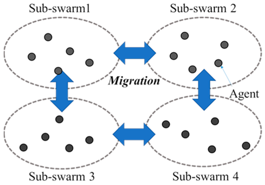
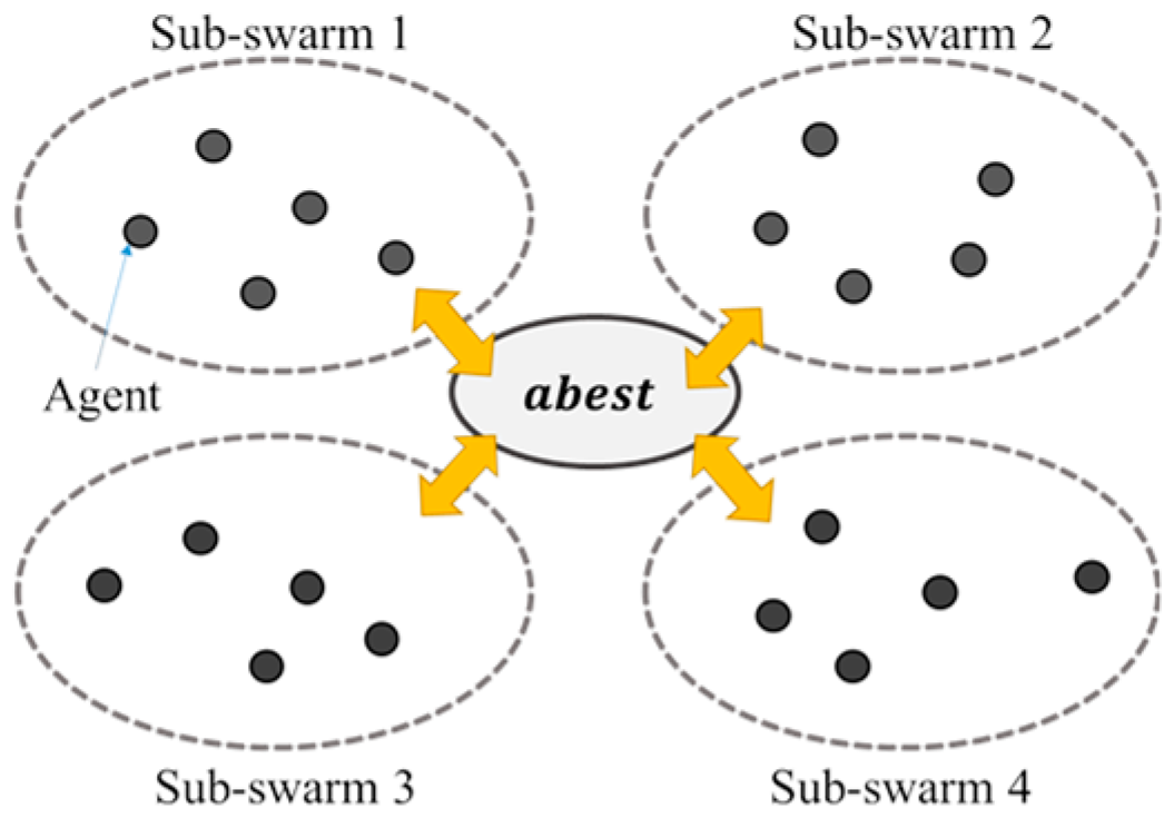
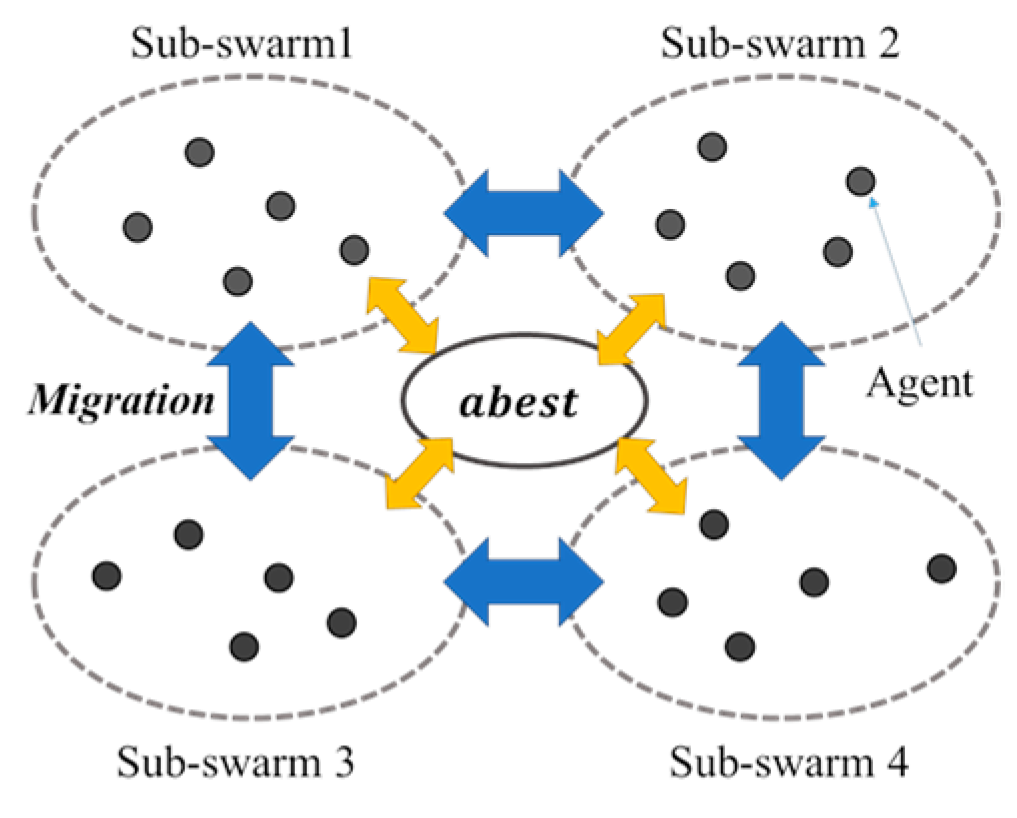
Conventionally, the migration model [18,19,21,23,24,25] (see Figure 3), the abest model [20,22] (see Figure 4), and a model using both migration and abest [26,31] (see Figure 5) has been considered in multi-population based evolutionary computation methods. The migration and abest model has been proposed by the authors because the smart city problem can be considered as one of the large-scale optimization problems [26]. Evolutionary computation methods with multiple searching points utilize only one population. On the contrary, the multi-population models divide searching individuals of one population into several sub-populations, and different searching process is performed at each sub-population. In addition, multi-population models exchange and replace searching individuals among sub-populations at certain intervals. The model shares the information of the best searching point of all sub-populations (abest) among all sub-populations in the abest model, and the combined migration and abest model. The various parameters of the models are shown below.

Figure 3.
A concept of a multi-population model using only migration (© 2018 IEEE [27]).

Figure 4.
A concept of a multi-population model using only abest (© 2018 IEEE [27]).
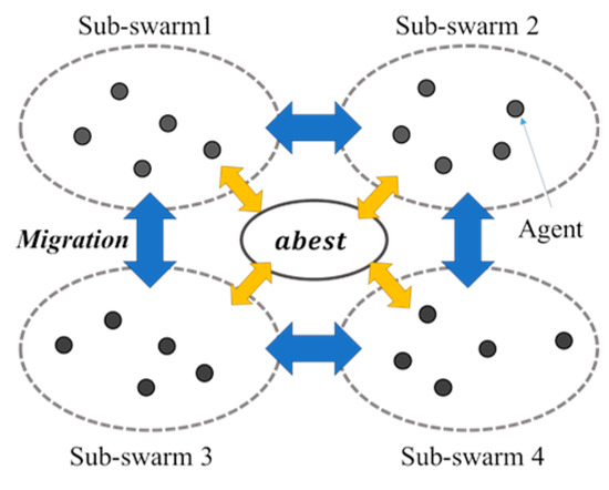
Figure 5.
A concept of a multi-population model using both migration and abest (© 2018 IEEE [27]).
- -
- The number of sub-populations: the number of sub-populations which performs GMBSO independently.
- -
- Migration topology: topological structures of sub-populations. Ring topology with 2, 4, 8, and 16 sub-populations (see Figure 6a–d), trigonal pyramid topology with four sub-populations, a cube topology with eight sub-populations, or hyper-cube topology with 16 sub-populations (see Figure 7a–c) can be utilized.
 Figure 6. Examples of ring topologies using various numbers of sub-populations (© 2018 IEEE [27]).
 Figure 7. Topologies with three and more connections using various numbers of sub-populations (© 2018 IEEE [27]).
 - -
- Migration interval: how often searching individuals migrate.
- -
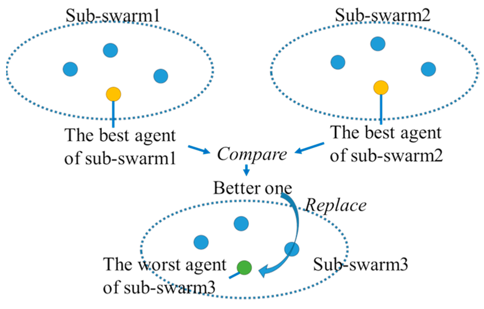
- Migration policy: the way to select searching individuals for replacement in the receiving sub-population and the way to select searching individuals for migration in the sending sub-population. The worst individual of the receiving sub-population is replaced by the best individual of the sending sub-populations (W-B) (see Figure 8) , a randomly selected individual of the receiving sub-population is replaced by the best individual of the sending sub-populations (R-B) , the best individual of the receiving sub-population is replaced by the best individual of the sending sub-populations (B-B), the worst individual of the receiving sub-population is replaced by a randomly selected individual of the sending sub-populations (W-R), a randomly selected individual of the receiving sub-population is replaced by a randomly selected individual of the sending sub-populations (R-R), the best individual of the receiving sub-population is replaced by a randomly selected individual of the sending sub-populations (B-R), the worst individual of the receiving sub-population is replaced by the worst individual of the sending sub-populations (W-W), a randomly selected individual of the receiving sub-population is replaced by the worst individual of the sending sub-populations (R-W), or the best individual of the receiving sub-population is replaced by the worst individual of the sending sub-populations (B-W), can be utilized .
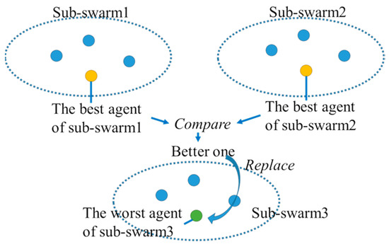 Figure 8. The concept of W-B policy (© 2018 IEEE [27]).
4.6. Update Equations of The Proposed MP-GMBSO with Migration
This paper proposes MP-GMBSO with migration. Equations for Fitness-based grouping, updating in order to apply information of “gbest” to , and equations for new individual generation are shown below.
Following Equation (12) is utilized for fitness-based grouping of MP-GMBSO.
where is a selected group number of individual in a sub-population , is the rank of individual in a sub-population , is the number of cluster in a sub-population , and is the number of sub-populations.
An equation for updating in order to apply information of “gbest” to is expanded for multi-population. There are two equations. One is for the only migration model. Another one is for the only abest model, and the combined migration and abest model.
- -
- the proposed MP-GMBSO with only migration model (see Figure 3):where is decision variable of the th individual in sub-population , and is decision variable of the best individual in sub-population .
- -
An equation for new individual generation is expanded for multi-population as shown below.
where is decision variable of the th newly generated individual in sub-population , and and are decision variable of the randomly selected two individuals of individual in sub-population .
5. Total Optimization of Energy Networks in a Smart City by Multi-Population Global-Best Modified Brain Storm Optimization with Migration
5.1. Cutout Transformation Function
Both discrete and continuous variables are dealt as the decision variables of the problem. In order to easily utilize evolutionary computation method, decision variables should be only continuous variables. Therefore, the authors utilize a cutout transformation function which changes both discrete and continuous variables to only continuous variables. In addition, the function can reduce the number of decision variables. Startup and shutdown status of facilities can be expressed as discrete variables (0 and 1). Operational values of facilities are expressed as continuous variables . Discrete variable is expressed as follows:
Shutdown status () of facilities cannot be searched effectively considering (16), because is equal to 0 if and only if is equal to 0. Hence, new continuous variables are utilized and the relationship between and are expressed as follows:
where is a minimum bound of (the minimum input/output value of a facility), is an maximum bound of (the upper input/output bound of a facility), is a parameter of for shutdown status of a facility, is a lower limit of , and is an upper limit of .
Both discrete and continuous variables are utilized in the problem. However, the function can change both the discrete and continuous variables to only continuous variables and the evolutionary computation can be easily utilized.
5.2. Reduction of Search Space
Conventionally and usually, from the current operating conditions of various facilities, search space is calculated using the maximum decrease/increase of energy output/input values of facilities, upper/lower bounds of energy output/input values of facilities. The authors have proposed a reduction method of search space considering not only characteristics of various facilities but also considering electric and natural gas hourly cost and hourly load characteristics, and smooth transition to the next day facility operation in weekdays. As an example, the reduction of search space of the heat storage tank is explained in this section. The upper and lower bounds of the stored heat energies are calculated from the initial condition () [11,12]. The bounds are calculated by the equations shown below:
where is the stored heat energies at hour , is the upper bound of stored heat energies in the heat storage tank at hour , is the lower bound of stored heat energies in the heat storage tank at hour , is the upper bound of heat input value at hour , is the lower bound of heat input value at hour , is heat output at hour , and is hourly heat loss.
Solid lines in Figure 9 show and and dash-dotted lines in Figure 9 show and . Using the same calculation concept of (20) and (21), and can be calculated using the opposite direction from hour considering smooth transition to the next day facility operation in weekdays. Finally, considering the upper and lower bounds explained above, the following (22) and (23) shows the reduced search space at each hour.
where is the upper bound of the stored heat energies in the heat storage tank in the reduced search space at hour , is the lower bound of the stored heat energies in the heat storage tank in the reduced search space at hour , is an upper bound of heat energies in the heat storage tank, and a lower bound of heat energies in the heat storage tank.
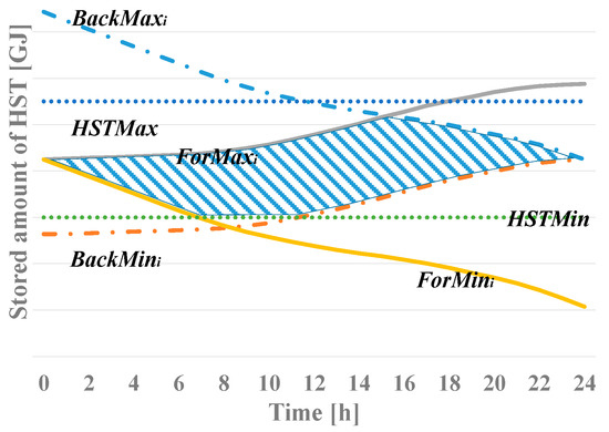
Figure 9.
A conventional search space (inside solid lines) and a reduced search space (shaded area) of a heat storage tank (© 2018 IEEE [27]).
The reduced search space is shown with a shaded area in Figure 9 considering not only characteristics of various facilities but also smooth transition to the next day facility operation in weekdays and heat hourly load characteristics. Consequently, the reduction of search space can realize effective search to the target problem.
5.3. The Proposed Total Optimization Algorithm of Smart City by MP-GMBSO with Migration
The proposed total optimization algorithm by MP-GMBSO with migration is shown below:
- Step 1
- Initialization: Divide all individuals into sub-populations. Generate initial individuals at each sub-population considering the reduced search space for a smart city.
- Step 2
- Calculate the objective function at all individuals in sub-populations.
- Step 3
- Clustering:
- Step 3-1
- Generate clusters using in all sub-populations.
- Step 3-2
- Calculate objective functions of all individuals in each cluster in all sub-populations.
- Step 3-3
- Rank individuals ascending order.
- Step 3-4
- The highest rank individuals at each cluster of all sub-populations are set as cluster centers. If randomly generate a new individual and replace a cluster center with the newly generated individual.
- Step 4
- Generation of new individual: When condition (9) is satisfied, information of “gbest” is applied to using (13) or (14). New individuals are generated considering several conditions explained in 4.1.2 using Equation (15).
- Step 5
- Selection:
- Step 5-1
- The objective function values are calculated for all individuals.
- Step 5-2
- The new individual is compared with the current individual with the same individual index. Keep the better one and the individual is stored as the current individual in all sub-populations.
- Step 6
- Evaluation: Calculate objective function values of individuals in all sub-populations. The best individual is updated when the objective function value of the individual is better than the current best individual.
- Step 7
- Individuals are migrated when the current iteration number reaches the migration interval which is pre-determined.
- Step 8
- the whole procedure is stopped and go to Step 9 when the current number of iterations reaches the maximum number of iterations which is pre-determined. Otherwise, go to Step 3 and repeat the procedures.
- Step 9
- The finally obtained objective function value and the best operational values are output as a final solution.
6. Simulations
6.1. Simulation Conditions
The proposed MP-GMBSO with migration is applied to a typical mid-sized city model referring to data of Toyama city in Japan. The numbers of models in each sector in the model are shown below. They are determined so that sector load ratios of the model are approximately the same as the sector load ratios of Toyama city [32]:
Industry model: 15, Building model: 50, Residential model: 45,000, Railroad: 1, Drinking water treatment plant: 1, Wastewater treatment plant: 1.
Usually, each smart city has each goal. Therefore, this paper considers the following three cases in order to consider different goals of smart cities:
- Case 1:
- a goal of a general smart city considering all three terms of the objective function equally,
- Case 2:
- a goal of an industrial park which usually concentrates only minimization of total energy cost
- Case 3:
- a goal of local government of a city which usually concentrates only minimization of CO2 emission.
The results of GMBSO based method are compared with those by the conventional DEEPSO, BSO, MBSO, and GBSO based methods. In addition, the results of the MP-GMBSO based method are compared with those by the originally proposed GMBSO based method with a single population, the MP-GMBSO based methods with only migration (the proposed method), with only abest, and with both migration and abest.
The following parameters are utilized for conventional DEEPSO:
- : 0.2, : 0.006, : 0.75, the initial weight coefficients (A, B, and C): 0.5, the number of clones: 1.
The following parameters are utilized for conventional BSO, MBSO, GBSO, and GMBSO:
- , , , , 0.2 (for MBSO, GMBSO), , (for GBSO and GMBSO).
The following parameters are utilized for the conventional and the proposed MP-GMBSO based method.
- -
- The initial weight coefficients of each term (D) is set to 0.5,
- -
- The number of sub-populations (NumSubPop): 2, 4, 8, and 16,
- -
- The total number of individuals (NumInd): 1280 (640 individuals/sub-population for 2 sub-populations, 320 individuals/sub-population for 4 sub-populations, 160 individuals/sub-population for 8 sub-populations, and 80 individuals/sub-population for 16 sub-populations), 640 (320 individuals/sub-population for 2 sub-populations, 160 individuals/sub-population for 4 sub-populations, 80 individuals/sub-population for 8 sub-populations, and 40 individuals/sub-population for 16 sub-populations), 320 (160 individuals/sub-population for 2 sub-populations, 80 individuals/sub-population for 4 sub-populations, 40 individuals/sub-population for 8 sub-populations, and 20 individuals/sub-population for 16 sub-populations), 160 (80 individuals/sub-population for 2 sub-populations, 40 individuals/sub-population for 4 sub-populations, 20 individuals/sub-population for 8 sub-populations, and 10 individuals/sub-population for 16 sub-populations), and 80 (40 individuals/sub-population for 2 sub-populations, 20 individuals/sub-population for 4 sub-populations, 10 individuals/sub-population for 8 sub-populations).
- -
- -
- Migration interval: 10 to 100 in 10 increments,
- -
- Migration policy: W-B, R-B, B-B, W-R, R-R, B-R, W-W, R-W, B-W.
The following parameters are utilized for all methods.
- -
- The number of trials: 50
- -
- The maximum iteration number for BSO, GBSO, MBSO, and GMBSO based methods: 2000
- -
- The maximum iteration number for DEEPSO based method is set to 1000
The conventional DEEPSO based method evaluates the objective function twice at each iteration for both new and clone individuals. Therefore, the maximum iteration number for DEEPSO is set to be half in order to keep the same number of objective function evaluation among all methods. Initial searching points are randomly generated for all methods. The simulation software has been developed using C language (gcc version 4.4.7) on a PC (Intel Xeon E5-2660 (2.20 GHz)).
6.2. Simulation Results
Firstly, the comparison of the mean, the minimum, the maximum, and the standard deviation of the objective function values for Case 1 among DEEPSO, BSO, MBSO, GBSO, and GMBSO based methods are shown in Table 2. Eighty individuals are utilized in Table 2. The number of individuals is set to 80 because the condition is the most severe for all methods. The results in the table are percentages of the objective function value when the mean of the objective function value by DEEPSO is set to 100%. It is verified that the mean, the minimum, the maximum, and the standard deviation of GMBSO based method can be the most reduced among all methods.

Table 2.
Comparison of the mean, the minimum, the maximum, and the standard deviation of the objective function value among conventional DEEPSO, BSO, MBSO, GBSO, and the proposed GMBSO based methods with 80 individuals. 1
Table 3 shows results of the mean ranks for Friedman test and p-value among the conventional DEEPSO, BSO, GBSO, MBSO, and GMBSO based methods. It is verified that there are significant differences at 0.05 significance level among all methods and the mean ranks by the GMBSO based method for each case are the best in Table 2.

Table 3.
Results of average ranks and Friedman Test through 50 trials among the conventional DEEPSO, BSO, GBSO, MBSO, and the proposed GMBSO based methods.
Secondly, the best multi-population model is investigated among three models, namely, only migration model, only abest model, or a model using both migration and abest. Table 4 shows comparison of the mean, the minimum, the maximum, the standard deviation, and the mean rank of the objective function value among various numbers of sub-populations, and topologies using both migration with the W-B policy and abest, only migration with the W-B policy, and only abest with 640 individuals for Case 1 through 50 trials and a p-value by Friedman test. Six hundred and forty individuals are utilized in the table because there is a possibility to obtain better results by the MP-GMBSO based method through previous studies. The results of Table 4 are calculated when the mean of the objective function value using one sub-population is set to 100%. It is verified that the mean, the minimum, the maximum, and the standard deviation can be the most reduced by the only migration model with 16 sub-populations (bold numbers). It can be considered that the GMBSO based method can focus on intensification more than the other methods including the multi-swarm DEEPSO based method with a model using both migration and abest [26]. Therefore, the only migration model is the best model especially for the proposed MP-GMBSO based model in order to balance diversification and intensification. In addition, the mean rank by the only migration model with 16 sub-populations is the best among all parameters in the table.

Table 4.
Comparison of the mean, the minimum, the maximum, the standard deviation, and average rank of the objective function value of the optimal objective function values among various numbers of sub-populations, and topologies using both migration with the W-B policy and abest, only migration with the W-B policy, and only abest with 640 individuals through 50 trials for Case 1 and a p-value by Friedman test. 1
Table 5 shows the mean, the minimum, the maximum, the standard deviation, and the average rank of the objective function value of the optimal objective function values of each migration model with 640 individuals through 50 trials for Case 1 and a p-value by Friedman test. It is verified that the mean, the minimum, the maximum value, and the average rank using only migration model are the best among all multi-population models. It is also verified that there are significant differences at 0.05 significance level among all parameters in Table 4.

Table 5.
The best values of the mean, the minimum, the maximum, the standard deviation, and the average rank of the objective function value of the optimal objective function values of each migration model with 640 individuals through 50 trials for Case 1 from Table 4 and a p-value by Friedman test. 1
Next, the best migration policy and topology are investigated in Table 6 when the only migration model is utilized. Table 6 shows comparison of the mean, the minimum, the maximum, the standard deviation values, and the average rank of the optimal objective function values using only migration model among various migration policies, various topologies, and various numbers of sub-populations with 640 individuals through 50 trials for Case 1 and a p-value by Friedman test. The results of the table are calculated when the average of the objective function value using one sub-population is set to 100%. It is studied that, using only migration, the results can be the most reduced by the “W-B” policy with 16 sub-populations and the ring topology (bold numbers), and the average rank by the “W-B” policy with 16 sub-populations and the ring topology is the best among all parameters in the table.

Table 6.
Comparison of the mean, the minimum, the maximum, the standard deviation values, and the average rank of the optimal objective function values using only migration model among various migration policies, various topologies, and various numbers of sub-populations with 640 individuals through 50 trials for Case 1 and a p-value by Friedman test. 1
Table 7 shows the best values of the mean, the minimum, and the maximum, the standard deviation values, and the average rank of the results calculated using optimal objective function values using only migration model of each migration policy with 640 individuals through 50 trials for Case 1 and a p-value by Friedman test. It is studied that the mean, the minimum, and the maximum values, and the average rank using W-B policy are the best among all migration policies (bold numbers). It is also studied that there are significant differences at 0.05 significance level among all parameters in Table 6.

Table 7.
The best values of the mean, the minimum, the maximum, the standard deviation values, and the average rank of the optimal objective function values using only migration model of each migration policy with 640 individuals through 50 trials for Case 1 from Table 6 and a p-value by Friedman test. 1
The best topology, the best number of individuals, and the best number of sub-populations are investigated in Table 8. Table 8 explains the comparison of the mean, the minimum, the maximum the standard deviation values, and average rank of the results calculated using objective function values using only migration model with the W-B policy among various topologies, various numbers of individuals, and various number of sub-populations and a p-value by Friedman test. When the number of individuals is 40 with 4 or 8 sub-population, the results include penalty value because dependent variables are out of allowable ranges. On the contrary, when the number of individuals is more than 80 or equal to 80, the results do not include penalty because dependent variables are inside allowable ranges. Especially, when the number of individuals is set to 320 with 16 sub-populations using ring topology, the mean, the minimum, and the maximum values can be the most reduced (bold numbers). Namely, the proposed method with such conditions can balance diversification and intensification the most effectively for the problem. In addition, the average rank is the best when the number of individuals is set to 320 with 16 sub-populations using ring topology among all parameters in Table 8.

Table 8.
Comparison of the mean, the minimum, the maximum, the standard deviation, and average rank of the objective function value of the optimal objective function values among various migration topologies with W-B policy, and various numbers of sub-populations using only migration with various number of individuals through 50 trials for Case 1 and a p-value by Friedman test. 1
Table 9 shows the best values of the mean, the minimum, the maximum, the standard deviation, and average rank of the objective function value of the optimal objective function values of each number of individuals with W-B policy using only migration and ring topology through 50 trials for Case 1 and a p-value by Friedman test. It is verified that the mean, the minimum, the maximum value, and the average rank with 320 individuals and 16 sub-populations are the best among all multi-population models (bold numbers). It is also verified that there are significant differences at 0.05 significance level among all methods.

Table 9.
The best values of the mean, the minimum, the maximum, the standard deviation, and average rank of the objective function value of the optimal objective function values of each number of individuals with WB policy using only migration and ring topology through 50 trials for Case 1 from Table 8 and a p-value by Friedman test. 1
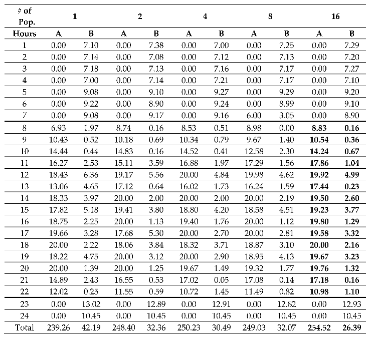
Table 10 and Table 11 investigate the above results (Table 2, Table 3, Table 4, Table 5, Table 6, Table 7, Table 8 and Table 9) from a facility operation point of view. In order to clarify these results, Table 10 shows comparison of the optimal operation of the facilities in an industrial model of Case 2 by MP-GMBSO using migration model, and W-B migration policy with ring topology when the number of individuals is set to 320 among various numbers of sub-populations. Column A indicates electric power output of a GTG and column B indicates electric power which is purchased from electric power utility at each hour. From 8 to 22 h, in the model, electric power which is purchased from electric power utility is expensive and electric power which is output of a GTG is inexpensive and purchased electricity is expensive. Hence, electric power which is purchased from electric power utility should be reduced and electric power which is output of a GTG should be increased from 8 to 22 h for reduction of energy cost. It is investigated that the electric power which is purchased from electric power utility can be the most reduced and electric power which is output of a GTG can be the most increased from 8 to 22 h by the proposed method (MP-GMBSO using migration model) with 16 sub-populations (bold numbers). Table 11 shows comparison of the best facility operation of an industrial model for Case 3 using only migration model, and W-B migration policy with ring topology when the number of individuals is set to 320 among various numbers of sub-populations. Electric power which is purchased from electric power utility should be reduced and electric power which is output of a GTG should be increased a whole day for reduction of CO2 emission in the model. It was verified that electric power which is purchased from electric power utility can be reduced and electric power output of a GTG can be increased at most a whole day by the proposed method with 16 (bold numbers).

Table 10.
Comparison of the best facility operation in an industrial model of Case 2 using migration model, and W-B migration policy with ring topology when the number of individuals is set to 320 among 1, 2, 4, 8, and 16 sub-populations.

Table 11.
Comparison of the best facility operation in an industrial model of Case 3 using migration model, and W-B migration policy with ring topology when the number of individuals is set to 320 among 1, 2, 4, 8, and 16 sub-populations. 1
Consequently, the proposed MP-GMBSO with only migration-based method with the W-B policy, the ring topology, 320 individuals, and 16 sub-populations is the most effective to the total optimization of energy networks in the smart city problem.
7. Conclusions
This paper proposes total optimization of energy networks in a smart city by multi-population global-best modified brain storm optimization (MP-GMBSO) with migration. A new evolutionary computation technique, called MP-GMBSO is proposed in order to obtain better results and the MP-GMBSO based method is proposed for total optimization of energy networks in a smart city. Effectiveness of the conventional GMBSO based method for total optimization of smart city by comparing with the conventional DEEPSO, BSO, MBSO, and GBSO based methods is verified. Moreover, effectiveness of the proposed MP-GMBSO based method for total optimization of smart city with migration is verified by comparing with the original GMBSO (MP-GMBSO with a sub-population) based method, and the MP-GMBSO based methods with various migration model (only using migration, only using abest, and using both migration and abest), various policies, various topologies, various numbers of individuals, and various numbers of sub-populations. It is verified that the quality of solution is the most improved by the proposed MP-GMBSO with migration-based method using the ring topology with 16 sub-populations and 320 individuals, and the W-B policy (the worst individual of a sub-population is replaced by the other sub-populations) among all multi-population parameters. Solutions by the proposed method can be changed by tuning weighting coefficients of the objective function considering the purpose of the target smart city.
As future works, several challenges can be considered. The smart city problem can be considered as one of the large-scale MINLP problems and it is hard to obtain solutions effectively. Therefore, firstly, state-of-the-art techniques of evolutionary computation will be applied in order to improve quality of solution. Secondly, various uncertainties of the problem will be considered. For example, uncertainty of renewable energy output depends on weather conditions. Uncertainty of various energy loads depends on various sector conditions. Hence, stochastic approaches such as a Monte Carlo simulation and robust optimization techniques should be applied. Thirdly, robustness of the proposed method will be investigated with various scale smart city models with different purposes.
Author Contributions
Conceptualization, M.S., Y.F.; methodology, M.S, Y.F.; software, M.S.; validation, M.S., Y.F.; analysis, M.S., Y.F.; investigation, M.S., Y.F., T.I., T.M.; writing—original draft preparation, M.S.; writing—review and editing, M.S., Y.F., T.I., T.M.; supervision, Y.F.
Funding
This work was supported by the Sasakawa Scientific Research Grant from the Japan Science Society.
Conflicts of Interest
The authors declare no conflicts of interest.
References
- Jaber, S.A.A. The MASDAR Initiative. In Proceedings of the First International Energy 2030 Conference, Abu Dhabi, UAE, 1–2 November 2006; pp. 36–37. [Google Scholar]
- Ministry of Economy, Trade, and Industry of Japan, Smart Community. Available online: http://www.meti.go.jp/english/policy/energy_environment/smart_community/ (accessed on 12 December 2018).
- Reconstruction Agency. Available online: http://www.reconstruction.go.jp/english/ (accessed on 20 December 2018).
- Henze, M. (Ed.) Activated Sludge Models ASM1, ASM2, ASM2d and ASM3; Scientific and Technical Report No. 9; IWA Publishing: London, UK, 2000. [Google Scholar]
- Makino, Y.; Fujita, H.; Lim, Y.; Tan, Y. Development of a Smart Community Simulator with Individual Emulation Modules for Community Facilities and Houses. In Proceedings of the IEEE 4th Global Conference on Consumer Electronics (GCCE), Osaka, Japan, 27–30 October 2015. [Google Scholar]
- Marckle, G.; Savic, D.A.; Walters, G.A. Application of Genetic Algorithms to Pump Scheduling for Water Supply. In Proceedings of the First International Conference on Genetic Algorithms in Engineering Systems: Innovations and Applications, Sheffield, UK, 12–14 September 1995. [Google Scholar]
- Suzuki, R.; Okamoto, T. An Optimization Benchmark Problem for Operational Planning of an Energy Plant. In Proceedings of the Electronics, Information, and Systems Society Meeting of IEEJ, TC7-2, Aomori, Japan, 5–7 September 2012. (In Japanese). [Google Scholar]
- Yasuda, K. Definition and Modelling of Smart Community. In Proceedings of the IEEJ National Conference, 1-H1-2, Tokyo, Japan, 24–25 March 2015. (In Japanese). [Google Scholar]
- Yamaguchi, N.; Ogata, T.; Ogita, Y.; Asanuma, S. Modelling Energy Supply Systems in Smart Community. In Proceedings of the Annual Meeting of the IEEJ, 1-H1-3, Tokyo, Japan, 24–25 March 2015. (In Japanese). [Google Scholar]
- Matsui, T.; Kosaka, T.; Komaki, D.; Yamaguchi, N.; Fukuyama, Y. Energy Consumption Models in Smart Community. In Proceedings of the Annual Meeting of the IEEJ, 1-H1-4, Tokyo, Japan, 24–25 March 2015. (In Japanese). [Google Scholar]
- Sato, M.; Fukuyama, Y. Total Optimization of Smart Community by Particle Swarm Optimization Considering Reduction of Search Space. In Proceedings of the 2016 IEEE International Conference on Power System Technology (POWERCON), Wollongong, NSW, Australia, 28 September–1 October 2016. [Google Scholar]
- Sato, M.; Fukuyama, Y. Total Optimization of Smart Community by Differential Evolution Considering Reduction of Search Space. In Proceedings of the IEEE TENCON 2016, Singapore, 22–25 November 2016. [Google Scholar]
- Sato, M.; Fukuyama, Y. Total Optimization of Smart Community by Differential Evolutionary Particle Swarm Optimization. In Proceedings of the IFAC World Congress 2017, Toulouse, France, 9–14 July 2017. [Google Scholar]
- Sato, M.; Fukuyama, Y. Total Optimization of Smart Community by Brain Storm Optimization. In Proceedings of the SICE Annual Conference 2018, Nara, Japan, 11–14 September 2018. [Google Scholar]
- Sato, M.; Fukuyama, Y. Total Optimization of Smart Community by Modified Brain Storm Optimization. In Proceedings of the 10th Symposium on Control of Power and Energy Systems (IFAC CPES2018), Tokyo, Japan, 4–6 September 2018. [Google Scholar]
- Sato, M.; Fukuyama, Y. Total Optimization of Smart Community by Global-best Brain Storm Optimization. In Proceedings of the GECCO 2018, Kyoto, Japan, 15–19 July 2018. [Google Scholar]
- Sato, M.; Fukuyama, Y.; Iizaka, T.; Matsui, T. Total Optimization of Smart Community by Global-best Modified Brain Storm Optimization. In Proceedings of the 11th International Joint Conference on Computational Intelligence (IJCCI 2018), Seville, Spain, 18–20 September 2018. [Google Scholar]
- Fukuyama, Y.; Chiang, H.D. A Parallel Genetic Algorithm for Generation Planning. IEEE Trans. Power Syst. 1996, 11, 955–961. [Google Scholar] [CrossRef]
- Lou, S.-H.; Wu, Y.-W.; Xiong, X.-Y.; Tu, G.-Y. A Parallel PSO Approach to Multi-Objective Reactive Power Optimization with Static Voltages Stability Consideration. In Proceedings of the IEEE Transmission and Distribution Conference and Exhibition, Dallas, TX, USA, 21–24 May 2006. [Google Scholar]
- Wang, D.; Wu, C.H.; Ip, A.; Wang, D.; Yan, Y. Parallel Multi-Population Particle Swarm Optimization Algorithm for the Uncapacitated Facility Location Problem using OpenMP. In Proceedings of the IEEE Congress on Evolutionary Computation (CEC) Conference, Hong Kong, China, 1–6 June 2008. [Google Scholar]
- Lorion, Y.; Bogon, T.; Timm, I.J.; Drobnik, O. An Agent Based Parallel Particle Swarm Optimization-APPSO. In Proceedings of the Swarm Intelligence Symposium (SIS), Nashville, TN, USA, 30 March–2 April 2009; pp. 52–59. [Google Scholar]
- Yazawa, K.; Tamura, K.; Yasuda, K.; Motoki, M.; Ishigame, A. Cluster-Structured Particle Swarm Optimization with Interaction and Adaptation. Electron. Commun. Jpn. 2011, 94, 9–17. [Google Scholar] [CrossRef]
- Lopes, R.A.; Pedrosa, R.C.; Campelo, F.; Guimaraes, G. A Multi-Agent Approach to the Adaptation of migration Topology in Island Model Evolutionary Algorithms. In Proceedings of the 2012 Brazilian Symposium on Neural Networks (SBRN), Curitiba, Brazil, 20–25 October 2012. [Google Scholar]
- Tang, J.; Lim, M.H.; Ong, Y.S.; Er, M.J. Study of migration topology in island model parallel hybrid-GA for large scale quadratic assignment problems. In Proceedings of the Eighth International Conference on Control, Automation, Robotics and Vision, Special Session on Computational Intelligence on the Grid, Kunming, China, 6–9 December 2014. [Google Scholar]
- Singh, H.; Srivastava, L. Optimal VAR control for Real Power Loss Minimization Voltage Stability Improvement using Hybrid Multi-Swarm PSO. In Proceedings of the International Conference on Circuit, Power and Computing Technologies (ICCPCT), Nagercoil, India, 18–19 March 2016. [Google Scholar]
- Sato, M.; Fukuyama, Y. Total Optimization of Smart Community by Multi-Swarm Differential Evolutionary Particle Swarm Optimization. In Proceedings of the IEEE Symposium Series on Computational Intelligence 2017 (SSCI 2017), Honolulu, HI, USA, 27 November–1 December 2017. [Google Scholar]
- Sato, M.; Fukuyama, Y.; Iizaka, T.; Matsui, T. Total Optimization of Energy Networks in a Smart City by Multi-Swarm Differential Evolutionary Particle Swarm Optimization. IEEE Trans. Sustain. Energy. [CrossRef]
- Shi, Y. Brain Storm Optimization Algorithm. In Proceedings of the International Conference in Swarm Intelligence, Chongqing, China, 12–15 June 2011; Lecture Notes in Computer Science. Volume 6728, pp. 295–303. [Google Scholar]
- Zhan, Z.; Zhang, J.; Shi, Y.; Liu, H. A Modified Brain Storm Optimization. In Proceedings of the 2012 IEEE Congress on Evolutionary Computation, Brisbane, Australia, 10–15 June 2012. [Google Scholar]
- El-Adb, M. Global-best brain storm optimization algorithm. Swarm Evol. Comput. 2017, 37, 27–44. [Google Scholar]
- Sato, M.; Fukuyama, Y.; Iizaka, T.; Matsui, T. Total Optimization of Smart City by Multi-population Global-best Modified Brain Storm Optimization. Proceedings of Joint 10th International Conference on Soft Computing and Intelligent Systems and 19th International Symposium on Advanced Intelligent Systems in conjunction with Intelligent Systems Workshop 2018 (SCIS&ISIS 2018), Toyama, Japan, 5–8 December 2018. [Google Scholar]
- Kanno, T.; Matsui, T.; Fukuyama, Y. Various Scenarios and Simulation Examples Using Smart Community Models. In Proceedings of the Annual Meeting of the IEEJ, Tokyo, Japan, 24–25 March 2015. (In Japanese). [Google Scholar]
© 2019 by the authors. Licensee MDPI, Basel, Switzerland. This article is an open access article distributed under the terms and conditions of the Creative Commons Attribution (CC BY) license (http://creativecommons.org/licenses/by/4.0/).

