Study of Precipitation Forecast Based on Deep Belief Networks

Abstract

Due to the impact of weather forecasting on global human life, and to better reflect the current trend of weather changes, it is necessary to conduct research about the prediction of precipitation and provide timely and complete precipitation information for climate prediction and early warning decisions to avoid serious meteorological disasters. For the precipitation prediction problem in the era of climate big data, we propose a new method based on deep learning. In this paper, we will apply deep belief networks in weather precipitation forecasting. Deep belief networks transform the feature representation of data in the original space into a new feature space, with semantic features to improve the predictive performance. The experimental results show, compared with other forecasting methods, the feasibility of deep belief networks in the field of weather forecasting.

1. Introduction

Whether it is sailing, navigation, agriculture, or travel, accurate weather forecasts are always needed. In recent years, science and technology have developed rapidly, the methods of weather data collection have become more diverse, and more and more meteorological data can be collected. It is always a challenge to improve the accuracy of traditional weather forecasting with large amounts of collected meteorological data. Information and computer technology have driven the development of massive data analysis capabilities, stimulated the interest of many research groups in using machine learning techniques for big data research, and pushed them to explore hidden correlations of weather forecasting with big data sets. Our mission is to build a powerful weather forecasting model that uses a large amount of weather data to reveal hidden data associations in the data and ultimately improve the accuracy of weather forecasts.

Precipitation forecasting is the core of the meteorological forecasting system. Improving the accuracy of precipitation prediction results is crucial to improving the forecast results of the entire meteorological forecasting system. Precipitation prediction is a complicated systematic project. The establishment of a meteorological forecasting system involves not only the collection and storage of data, such as climate, geography, and environment, but also accurate predictions based on the obtained data. This has always been a hot issue in the field of meteorological forecasting. Currently, precipitation data is collected mainly in the following three ways: Measurement of rain ganges, satellite-derived rainfall data, and radar rainfall estimation [1]. The three acquisition methods have their own advantages and disadvantages. Although the precipitation data obtained by rain ganges is accurate, it only reflects the precipitation in a small area, with poor spatial representativeness. Precipitation data from satellites and radars have a high coverage area, but the data accuracy is not very satisfactory. Therefore, the precipitation data collected by the automatic weather station is the most reliable data among the precipitation observation data. However, due to the limitation of the geographical environment and funds, the automatic weather station cannot be evenly distributed, so the observation data inevitably appear unevenly distributed in time and space. Although the accuracy of precipitation data from rain ganges is great, the data lacks continuity in time and space, and it is difficult to reflect the overall trend of regional climate change. Therefore, the existing ground weather station cannot meet the increasingly demanding accuracy requirements of today’s precipitation products, and there is an urgent need for research breakthroughs.

Nowadays, how to improve the accuracy of forecasts is a hot and difficult topic in the field of forecasting. In the era of big data, how to use the large amount of weather data collected to improve the accuracy of the traditional weather forecast rate has always been a challenge of weather forecasting. Our task is to create a powerful weather forecasting model that uses a large amount of weather data to reveal hidden data associations in the weather data and eventually improve the accuracy of the weather forecast.

2. Related Work

For the requirement of high quality and high resolution precipitation products, the National Oceanic and Atmospheric Administration (NOAA), National Severe Storms Laboratory (NSSL), and the National Weather Service (NWS) Hydrology Development Office jointly developed the NMQ plan (The National Mosaic and Multisensor QPE Project), developed real-time quantitative precipitation estimations and introduced all kinds of high resolution (QPE) products [2,3]. Meanwhile, the free MPing software (Version 2.0) developed is used to collect meteorological data of the public’s participation in the perception, collects the meteorological information around the public’s location, and transmits it to the server through the MPing software installed in smart mobile devices to assist the dual-polarization radar data.

The weather forecasting method has achieved long-term development in recent years, with a lot of scholars establishing some prediction models about precipitation forecasting, such as the ARIMA (Autoregressive Integrating Moving Average) model [4,5,6,7], Markov model [8,9,10], gray theory-based prediction model [11], and so on. These studies have contributed to the development of the precipitation forecast. However, there are some shortcomings that should be further studied. The Markov model and gray model-based forecasting model are more suitable for the exponential growth of rainfall. The prediction error of extremum is larger in the ARIMA model. Deep learning is a novel machine learning method proposed in the field of artificial intelligence in recent years. Deep learning can be an effective big data processing method by training big data, mining and capturing the deep connection between big data to improve the classification and prediction accuracy. In addition, the deep learning model training is faster, and it shows better performance than the general growth of the method with the increase of training samples. The weather forecast model based on deep learning is better equipped to overcome the shortcomings of the existing forecast methods. Due to the achievements of deep learning algorithms in various fields, more and more people have tried to use deep learning algorithms in the field of weather forecasting, and some progress has been made. Researchers have done a lot of important work in this area. For example, Hsu demonstrated the potential of identifying the structure and parameters of three-layer feed forward Artificial Neural Network models (ANN), and it provided a better representation of the rainfall-runoff relationship of the medium-size Leaf River basin near Collins, Mississippi, than the linear ARMAX (autoregressive moving average with exogenous inputs) and the conceptual SAC-SMA (Sacramento soil moisture accounting) model [12]. Liu proposed that the deep neural network (DNN) model may granulate the features of the raw weather data layer by layer to process massive volumes of weather data [13]. Belayneh and Adamowski evaluated the effectiveness of three data-driven models, the artificial neural networks (ANNs), support vector regression (SVR), and wavelet neural networks (WN), by using the standard precipitation index for forecasting drought conditions in the Awash River Basin of Ethiopia [14]. Afshin proposed a long term rainfall forecasting model using the integrated wavelet and neuro-fuzzy long term rainfall forecasting model [15]. The other study has shown the applicability of an ensemble of artificial neural networks and learning paradigms for weather forecasting in southern Saskatchewan, Canada [16]. Valipour forecasted annual precipitation based on a non-linear autoregressive neural network (NARNN) and non-linear inputbility of an ensemble of artificial neural networks with historical precipitation data, and the results showed that the accuracy of the NARNNX (non-linear autoregressive neural network with exogenous input) was better than that of the NARNN and NIO (non-linear input–output), based on values of r [17]. Ha used DBN (Deep belief networks) to improve precipitation accuracy with the past precipitation, temperature, and parameters of the sun and moon’s motion in Seoul. Their experiment proved that the DBN performed better than the MLP (Multi-Layer Perceptron) for forecasting precipitation [18].

Under the background of meteorological big data, deep learning technology can use massive multi-source meteorological data and take sufficient observation data as training samples to ensure the accuracy of the weather forecasting model. The deep learning model can explore the inherent data relationship between meteorological elements in depth, and establish a more accurate proxy model of complex mechanism models between weather conditions and meteorological elements.

Based on the above reasons, this study proposes an effective rainfall forecasting model based on deep belief networks. The purpose of our survey is to explore the potential of deep learning technologies for weather forecasting. We will explore several deep learning models for weather forecasting, such as support vector machine (SVM), support vector machines based on particle swarm optimization (PSO-SVM), and deep belief network models (DBN). The remainder of this paper is organized as follows: In the following section an introduction to PSO-SVM and DBN are presented. In the Simulation and Discussion sections, we describe the features of the data used for predictions of precipitation, as well as the comparative results among these prediction models. The last part is the Results section of this paper, and it presents some discussions of our model and the last section states our conclusions.

3. Material and Methods

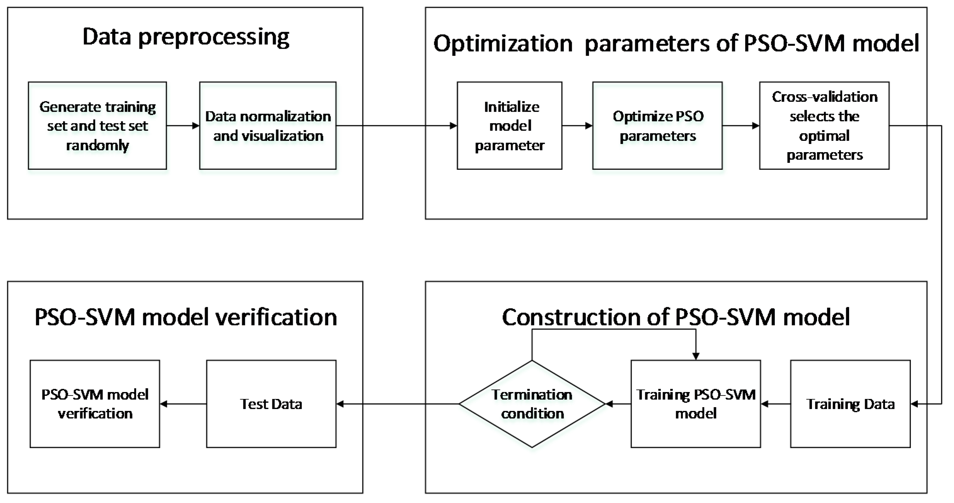
3.1. SVM Based on the PSO

The support vector machine with particle swarm optimization (PSO-SVM) was used to analyze and process the precipitation data in the literature [19]. SVM has many unique advantages in solving small sample, nonlinear, and high dimensional pattern recognition problems. It is given by Vapnik in 1995 [20]. An artificial neural network model based on hybrid genetic algorithm and particle swarm optimization (HGAPSO) optimization was proposed as an intelligent method for predicting natural depletion of asphaltenes [21]. SVM is a classification method based on statistical learning and Vapnik–Chervonenkis (VC) dimensional theories [22].

The literature [19] introduced the particle swarm optimization algorithm to search the training parameters in global space to improve the accuracy of the model for precipitation prediction. A combination of the PSO algorithm and SVM model can effectively solve the parameter selection problem of the SVM algorithm. It used the PSO algorithm to optimize the parameters in the literature [19]: Initialize parameters of particle swarm optimization include the population size, maximum iteration number, and the parameters, C and g. Particle swarm optimization is adopted to search the optimal solution of particles in global space by using the cross-validation algorithm. Inputting the training data into the SVM model with the optimal parameters allows the trained PSO-SVM model to be obtained. Figure 1 is the flowchart of the PSO-SVM model.

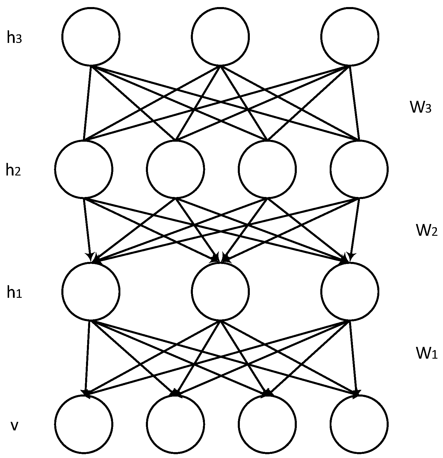
3.2. Deep Belief Network

Deep belief networks are developed based on multi-layer restricted Boltzmann machines (RBMs) [23]. The algorithm is composed of a multi-layer restricted Boltzmann machine (RBM) and a BP (back propagation) network. The top layer of the BP network fine-tunes the RBM layers below to improve the performance of the algorithm. The restricted Boltzmann machine is divided into two parts. The first part is a visible layer, V, which is used to receive the feature data, and the second part is a hidden layer, H, which is used as a feature detector, including abstract features of the data [24]. This is illustrated in the Figure 2 below.

The study [25] showed that RBMs can be stacked and trained in a greedy manner to form so-called deep belief networks (DBN). DBNs learn to extract a deep hierarchical representation of the training data. The joint distribution between the input vector, $x$, and the $l$ hidden layers, $h^k$, is as follows:

$$P(x,h^1,\cdots ,h^l)=({\displaystyle \prod _{k=0}^{l-2}P(h^k|h^{k+1})})P(h^{l-1},h^l)$$

(1)

where $x=h^0$, and $P(h^{l-1},h^l)$ is the V-H joint distribution in the top-level. RBM $P(h^{k-1}|h^k)$ is a conditional distribution for the units of the visible layer conditioned on the units of the hidden layer of the RBM at the level, $k$.

This paper uses a fast layer learning algorithm for deep belief nets proposed by Hinton [26]. The principle of greedy layer-wise unsupervised training can be applied to DBNs with RBMs as the building blocks for each layer [25,27]. The process is as follows:

Step 1.

Train the raw input, $x=h^{(0)}$, as the first RBM layer. The first layer is its visible layer.

Step 2.

The hidden layer of the first RBM layer is used as the visual layer of the second RBM layer. The output of the first layer is used as the input of the second layer. This representation can be chosen as being the samples of $p(h^{(1)}|h^{(0)})$ or mean activations of $p(h^{(1)}=1|h^{(0)})$.

Step 3.

Take the transformed samples or mean activations as training examples to train the second layer as an RBM.

Step 4.

Repeat Step 2 and Step 3, upward of either samples or mean values each iterate.

Step 5.

When the training period is reached, or this satisfies the stop condition, end the iteration.

In this paper, we focus on fine-tuning by supervised gradient descent (SGD). We use a logistic regression classifier (LRC) to classify the input vector, $x$, based on the output of the last hidden layer, $h^{(l)}$, of the DBN. Fine-tuning is then performed via SGD of the negative log-likelihood cost function.

The program module is shown in Figure 3.

Each module in Figure 3 is described as follows:

(1) Import data sets

Import preprocessed weather data from the database. The data is divided into three data sets: Training data, verification data, and test data. Store data and data labels into data_set and data_label_set.

(2) Conversion data format

The format of the read data is a matrix, which requires further processing. Therefore, the data set can be loaded into the shared variable, reducing the consumption of continuously copied data, and improving the efficiency of the program. At the same time, the label of the data set is converted into a one-dimensional vector to facilitate the program calculation.

(3) Establish DBN model

Initialize the parameters. Set the learning rate, fiftytune_lr = 0.1, the maximum iteration number of pre-training, pretraining_epochs = 100, the learning rate of pre-training, pretrain_lr = 0.01, the maximum iteration number of training, training_epochs = 100, and the batch data size, batch_size = 10.

(4) Pre-training model

Divide the training data into several minbatches to shorten the overhead of building models. At the same time, we give an index to every minbatch. An RBM is trained on the minbatch according to the index value, and establishes the function model. Through continuous iteration, we can build function models in all minbatches, so we get a series of model functions.

(5) Fine-tuning the model

Create three functions to complete the fine-tuning of the model. The three functions calculate the loss function on a batch of the training, verification, and test set. During the fine tuning, we perform random gradient descent through the MLP to find the best DBN model with the best loss value.

(6) Results and Models

We test the test data with the best DBN model and get the test results. Get the best test accuracy on the test set and the time spent in the pre-training and fine-tuning phases of the program.

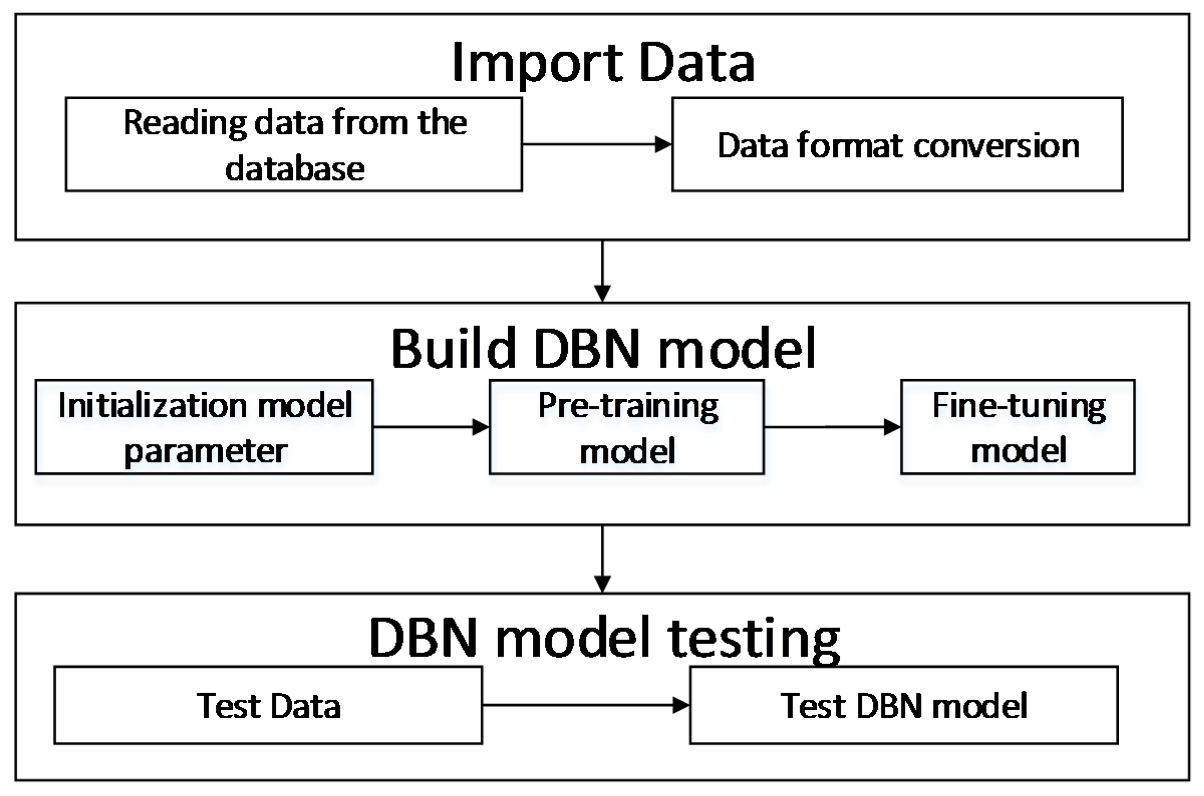
4. Results and Discussion

4.1. Data Collection and Preprocessing

For this study, we use the one-year ground-based meteorological data from Nanjing Station (NO. [58238]). The data sets are downloaded from the China meteorological data network, and the information of the Nanjing station is showed in

Table 1. Station information of China Ground Weather Station.

Province	Station No.	Station Name	Latitude	Longitude	Air Pressure Sensor Pull Height (m)	Observatory Height (m)
Jiangsu	58238	Nanjing	31.56	118.54	36.4	35.2

.

The dataset contains atmospheric pressure, sea level pressure, wind direction, wind speed, relative humidity, and precipitation. Data is collected every three hours. As shown in

Table 2. Original meteorological data.

PRS (hPa)	PRS_Sea (hPa)	WIN_D (°)	WIN_S (0.1 m/s)	TEM (°C)	RHU (%)	PRE_1h (mm)
1031.2	1035.8	89	2.5	77	2	0
1030.8	1035.4	113	2.9	61	6.4	0
1027.3	1031.9	153	2.1	49	8.3	0
1026.2	1030.8	122	2	55	7.1	0
$⋮$	$⋮$	$⋮$	$⋮$	$⋮$	$⋮$	$⋮$
1027.1	1031.7	121	0.7	71	4.1	0

, the first line is the attributes of the original meteorological data set; PRS represents atmospheric pressure, PRS_Sea is the sea level pressure, WIN_D is the wind direction, WIN_S is the wind speed, TEM is the temperature, RHU is the relative humidity, and PRE_1h is the one hourly precipitation.

4.2. Data Normalization

In general, data need to be normalized when the sample data are scattered and the sample span is large, so that the data span is reduced to build the model and prediction. In the DBN modeling, to improve the accuracy of prediction and smooth the training procedure, all the sample data were normalized to fit them in the interval [0,1] using the following linear mapping formula: $(-x_{id\max }^{},x_{id\max }^{})$

$$X^{\prime }=\frac{x_i-x_{\min }}{x_{\max }-x_{\min }},\hspace{1em}i=1,2,3\cdots ,N$$

(2)

where $X^{\prime }$ is the mapped value; x is the initial value from the experimental data; $N$ is the total number; $x_i$ is $i$ of input data; and $x_{\max }$ and $x_{\min }$ denote the maximum and minimum values of the initial data, respectively.

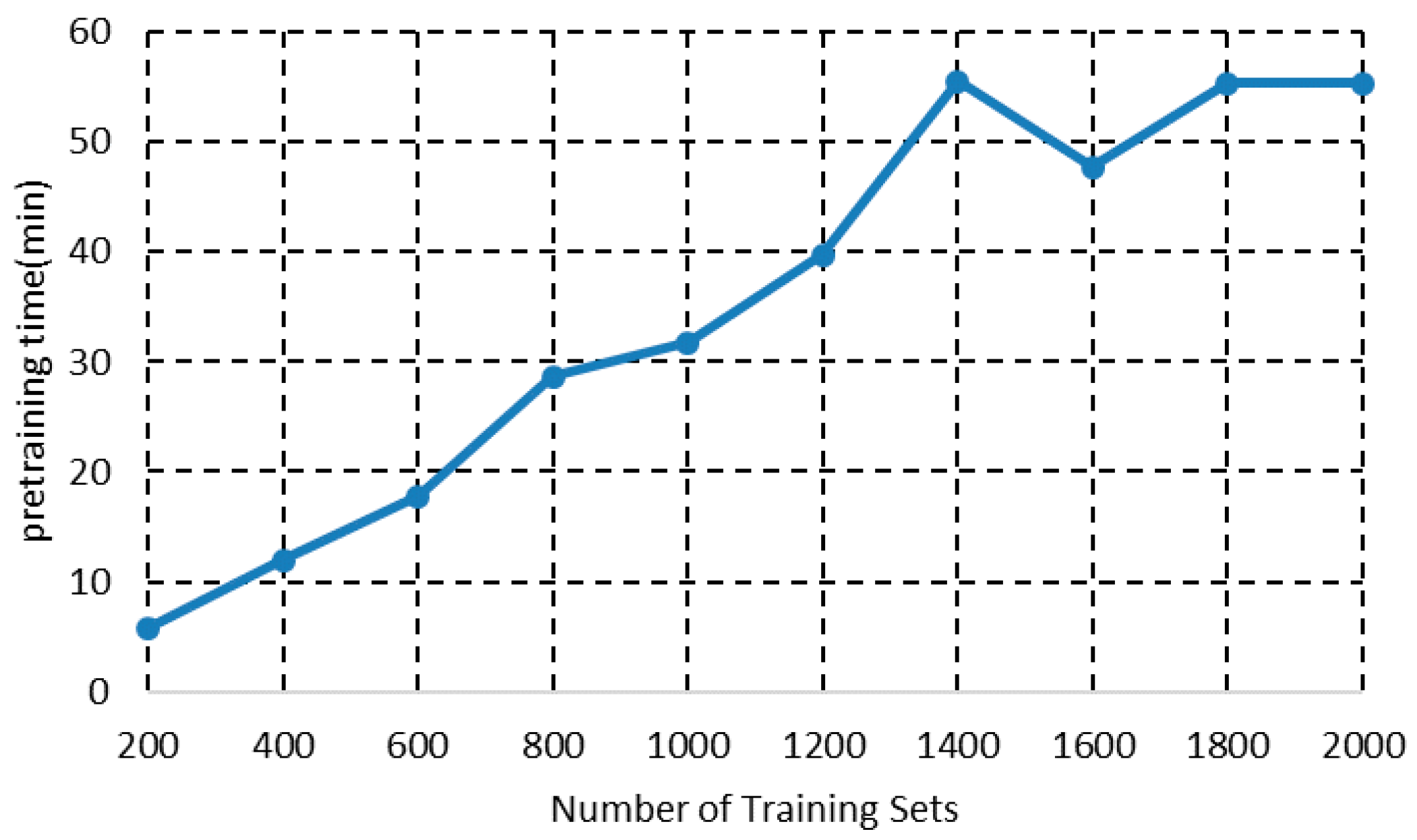
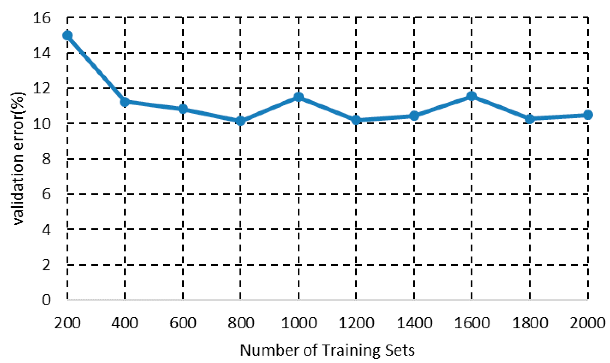
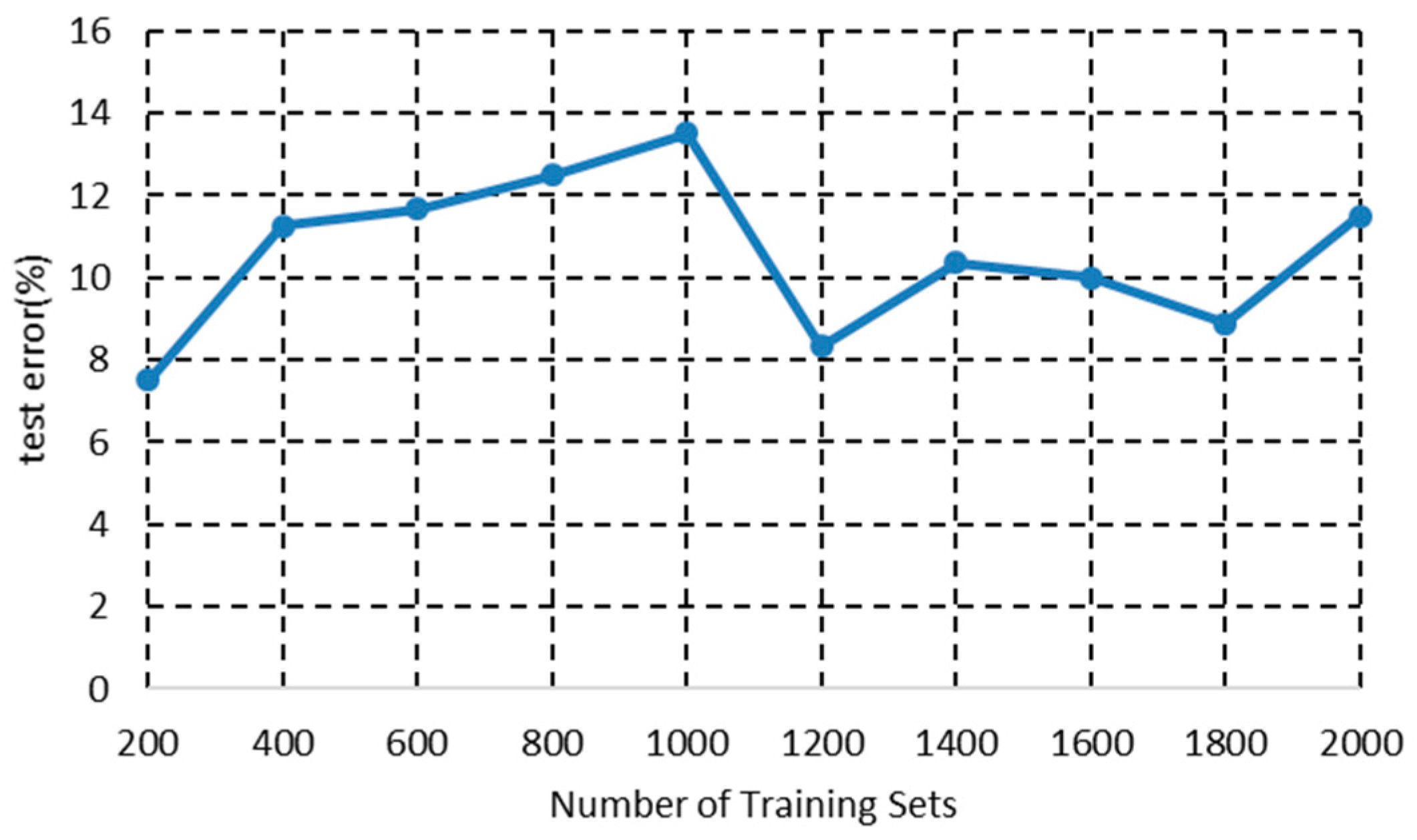
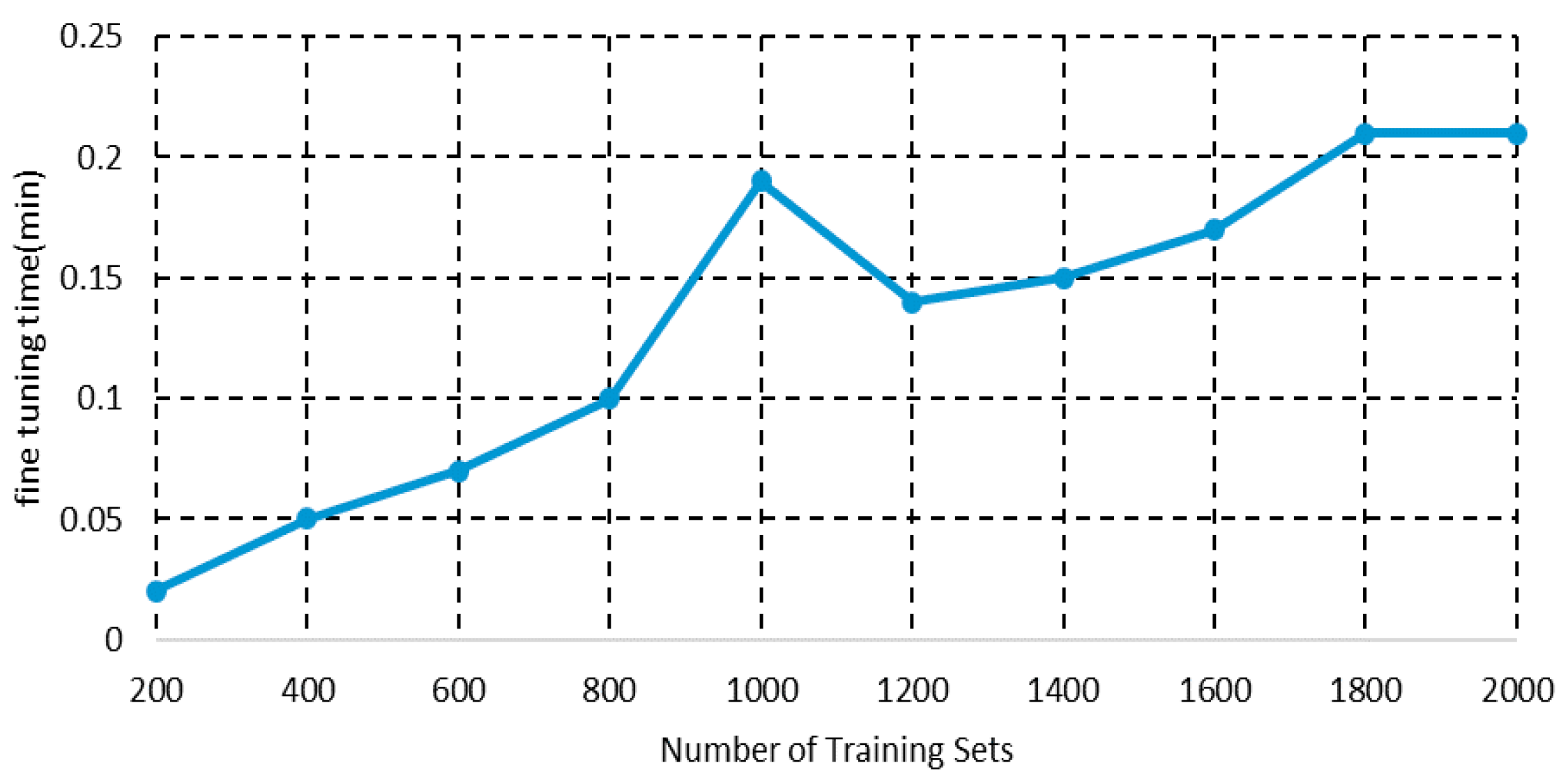
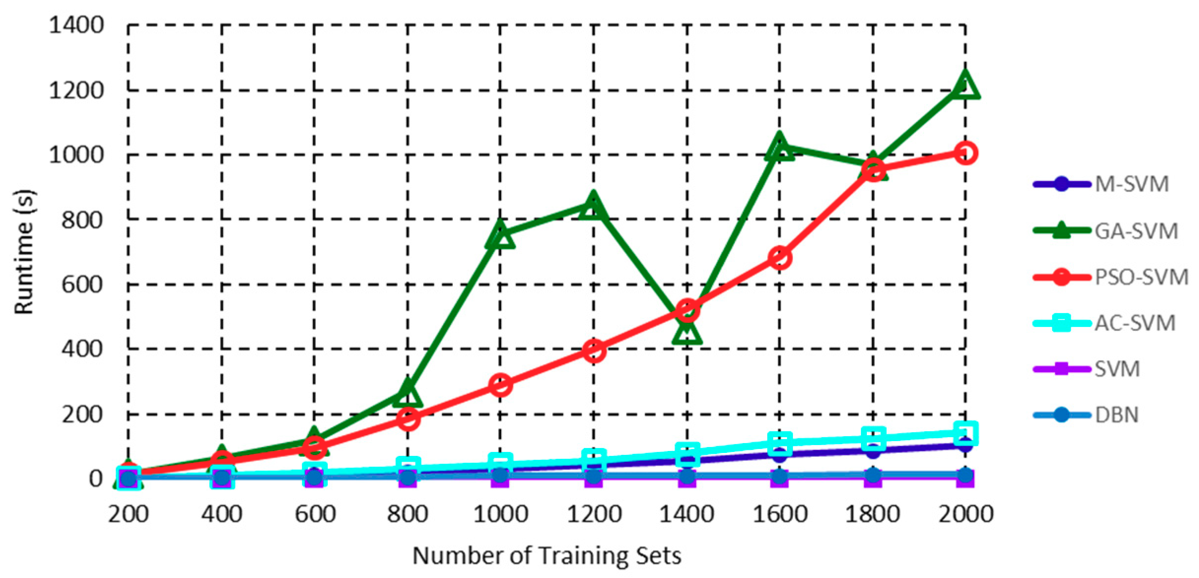
4.3. Algorithm Validation

For the assessment of the algorithms’ results, calibration and external testing were carried out. In the calibration assessment, the models were developed using the training set and validated with the same one. Finally, the prediction results were obtained via an external validation, training and testing the models with the training and test datasets, respectively.

In this paper, the number of samples was 200, 400, 600, 800, 1000, 1200, 1400, 1600, 1800, and 2000. For each type of sample number, 80% of the data were randomly selected as the training set for constructing the algorithm model, and the remaining 20% of the data were used as the test set to validate the model accuracy.

From the analysis in the third section, we know the process of establishing the DBN model. We used the data processing method described in the third section to establish a DBN model for the pre-processed meteorological data. According to the data processing flow, the following data results are obtained.

Figure 4 shows the time required for the pre-training part with the number of samples changes. The figure shows that as the number of samples increases, the time required for pre-training increases too. When the number of samples is small, the curve has a linear relationship with the number of samples; when the number of samples reaches a certain size, such as 1400, 1800, and 2000 points, the time consumed is almost the same, but the training time of 1600 points is less than the 1400 point and 1800 point, and it is higher than the pre-training time of 1200 samples.

We finetuned the pre-training model that was obtained, used the verification set to obtain the error rate of the fine-tuned model, and selected the model with the smallest error rate as the best model. The result in Figure 5 is the best error rate obtained by verifying the prediction effect of the model by the verification set. When the number of samples gradually increases, the error of the pre-training model in the validation set gradually becomes stable. The error rate of the 200 point is the highest compared to the number of other samples. Because of the small size of the data set, it cannot establish a better pre-training model, so the error is higher than others. The subsequent curve changes smoothly and the error rate is stable at around 11%.

The curve in Figure 6 is the error rate curve obtained by training the test data on the model. The average error rate of the verification data is 11.17%, and the average error rate of the test data is 10.55%, which is lower than the error rate of training and verification data. The lowest error rate is at the 200 point. Due to the small sample size, the error rate at this point changes significantly. The error rate of the 1600 point is 10%. Although the pre-training time of this point is shorter than others, the error rate is not higher than that of other sample numbers. On the whole, the error rate of the small sample size of the data is larger than the error rate when the sample size of the data is large.

Figure 7 shows the time curve of the model training test data. With the increase of the number of samples, the time of the model training test data gradually increases. Only the time of 1000 points is slightly higher than the other points around.

Experiments show that the application of DBN is effective and feasible in the field of precipitation prediction.

The deep confidence network used in this article is implemented in the python platform using the theano package, which makes the program have very good scalability and facilitates the application of the program. The python platform has a large number of open source frameworks that can be applied to big data processing, and has a very broad prospect in the field of big data processing.

As shown in Figure 8, the blue line indicates the time required for DBN to make predictions. M-SVM is based on mesh optimization, GA-SVM is based on genetic algorithm optimization, and PSO-SVM is based on particle swarm optimization. Because it consumes a lot of time for the model establishment in the previous period, when the model is used for prediction, the time consumed is lower than all the SVM methods used to establish the model. Additionally, it is guaranteed to have a certain accuracy rate. In practice, it is feasible to establish a good model using historical data in advance, and it will not affect the result of predicting precipitation. Therefore, an SVM method with excellent performance can be used when the data set is small, and the high efficiency of the DBN method can be used for large-scale data sets.

Data preprocessing can improve the running results of the model. After data preprocessing, the result of the operation is relatively smooth, so it is very necessary to preprocess the source data. According to Figure 4, Figure 5, Figure 6, Figure 7 and Figure 8, in terms of the test set’s training accuracy, the accuracy of the DBN model is more stable than that of the PSO-SVM model. However, because the steps for building the model are different, the PSO-SVM optimizes the parameters (C, g) on the training set. It then uses the value of (C, g) on the test set to recreate the model. DBN establishes and fine-tunes the model on the training set. Then, the model is directly invoked on the test set, which saves the time for building the model. Therefore, in the application of large data volume, the model can be trained in advance and the response speed is faster.

5. Conclusions

The result of this study is expected to contribute to weather forecasting for wide range of application domains, including flight navigation, agriculture, and tourism.

This paper focuses on the increasing size of meteorological datasets, discusses the application of big data processing technology in the meteorological field, and proposes a meteorological precipitation forecasting method based on deep learning. This method is based on the deep belief network and establishes a statistical model between precipitation features and other meteorological elements based on historical meteorological data. It uses meteorological big data to train the model, fully tap potential features between data elements, and achieve precipitation forecast based on meteorological data. The validity of the DBN model in precipitation forecasting was verified by comparison with the classical machine learning prediction method. The research shows that the forecasting method based on deep learning can overcome the shortcomings of traditional forecasting methods, especially in the context of big data, and it can better tap the value of air, like big data, and improve the application effect of meteorological big data.

References

1. Pan, Y.; Shen, Y.; Yu, J.J.; Xiong, A.Y. An experiment of high-resolution gauge-radar-satellite combined precipitation retrieval based on the Bayesian merging method. J. Meteorol. 2015, 73, 177–186. [Google Scholar] [CrossRef]
2. Kondragunta, C.; Seo, D.J. Toward Integration of Satellite Precipitation Estimates into the Multisensor Precipitation Estimator Algorithm. Available online: https://www.google.com.hk/url?sa=t&rct=j&q=&esrc=s&source=web&cd=2&ved=2ahUKEwj2jrnJ4Z3dAhUOHXAKHWqoAD8QFjABegQICBAC&url=https%3A%2F%2Fams.confex.com%2Fams%2Fpdfpapers%2F71020.pdf&usg=AOvVaw3O8d6_9aKJB8DEx0731J-P (accessed on 3 September 2004).
3. Seo, D.J. Real-time esimation of rainfall fields using radar rainfall and rain gage data. J. Hydrol. 1998, 208, 37–52. [Google Scholar] [CrossRef]
4. Lin, F.H.; Liang, L.I.; Chen, L.B. Theoretical Forecast Model of Rainfall and Its Application in Engineering. China Railway Sci. 2002, 23, 62–66. [Google Scholar]
5. Qian, H.; Li, P.Y.; Wang, T. Precipitation Predictionon Shizuishan City in Ningxia Province Based on Moving Average and Weighted Markov Chain. J. North China Inst. Water Conserv. Hydroelectr. Power 2010, 31, 6–9. [Google Scholar]
6. Cui, L.; Chi, D.C.; Qu, X. Application of Smooth and Steady Time Series Based on Wavelet Denoising in Precipitation Prediction. China Rural Water Hydropower 2010, 34, 30–32, 35. [Google Scholar]
7. Cui, D.Y. Application of Combination Model in Rainfall Prediction. Comput. Simul. 2012, 29, 163–166. [Google Scholar]
8. Wang, T.; Qian, H.; Li, P.Y. Prediction of Precipitation Based on the Weighted Markov Chain in Yinchuan Area. South-to-North Water Transf. Water Sci. Technol. 2010, 8, 78–81. [Google Scholar] [CrossRef]
9. Wang, Y.; Mao, M.Z. Application of Weighted Markov Chain Determined by Optimal Segmentation Method in Rainfall Forecasting. Stat. Decis. 2009, 11, 17–18. [Google Scholar] [CrossRef]
10. Zhong, Y.J.; Li, J.; Wang, L. Precipitation Predicting Model Based on Improved Markov Chain. J. Univ. Jinan (Sci. Technol.) 2009, 23, 402–405. [Google Scholar] [CrossRef]
11. Ren, Y.; Xu, S.M. Gray neural network combination model Application of Annual Precipitation Forecast in Qingan County. Water Sav. Irrig. 2012, 9, 24–25, 29. [Google Scholar]
12. Hsu, K.L.; Gupta, H.V.; Sorooshian, S. Artificial neural network modeling of rainfall-runoff process. Water Resources Res. 1995, 31, 2517–2530. [Google Scholar] [CrossRef]
13. Liu, J.N.K.; Hu, Y.; He, Y.; Chan, P.W.; Lai, I. Deep Neural Network Modeling for Big Data Weather Forecasting, Information Granularity, Big Data, and Computational Intelligence; Springer International Publishing: Cham, Switzerland, 2015; pp. 389–408. [Google Scholar]
14. Belayneh, A.; Adamowski, J. Standard Precipitation Index Drought Forecasting Using Neural Networks, Wavelet Neural Networks, and Support Vector Regression. In Applied Computational Intelligence and Soft Computing; Article ID 794061; Hindawi Publishing Corporation: New York, NY, USA, 2012; 13p. [Google Scholar]
15. Afshin, S. Long Term Rainfall Forecasting by Integrated Artificial, Neural Network-Fuzzy Logic-Wavelet Model in Karoon Basin. Sci. Res. Essay 2011, 6, 1200–1208. [Google Scholar]
16. Maqsood, I.; Khan, M.R.; Abraham, A. An ensemble of neural networks for weather forecasting. Neural Comput. Appl. 2004, 13, 112–122. [Google Scholar] [CrossRef] [Green Version]
17. Valipour, M. Optimization of neural networks for precipitation analysis in a humid region to detect drought and wet year alarms. Meteorol. Appl. 2016, 23, 91–100. [Google Scholar] [CrossRef]
18. Ha, J.H.; Yong, H.L.; Kim, Y.H. Forecasting the Precipitation of the Next Day Using Deep Learning. J. Korean Inst. Intell. Syst. 2016, 26, 93–98. [Google Scholar] [CrossRef] [Green Version]
19. Du, J.L.; Liu, Y.Y. A Prediction of Precipitation Data Based on Support Vector Machine and Particle Swarm Optimization (PSO-SVM) Algorithms. Algorithms 2017, 10, 57. [Google Scholar] [CrossRef]
20. Vapnik, V.N. The Nature of Statistical Learning Theory, 1st ed.; Springer: New York, NY, USA, 1995; ISBN 978-1-4757-2442-4. [Google Scholar]
21. Ahmadi, M.A.; Golshadi, M. Neural network based swarm concept for prediction asphaltene precipitation due to natural depletion. J. Pet. Sci. Eng. 2012, 98–99, 40–49. [Google Scholar] [CrossRef]
22. Vapnik, V.N.; Chervonenkis, A. On the Uniform Convergence of Relative Frequencies of Events to Their Probabilities, Theory of Probability and Its Applications; Springer International Publishing: New York, NY, USA, 1971; pp. 264–280. ISBN 978-3-319-21851-9. [Google Scholar]
23. Bengio, Y.; Delalleau, O. On the expressive power of deep architectures. In International Conference on Algorithmic Learning Theory; Springer: Berlin/Heidelberg, Germany, 2011; pp. 18–36. [Google Scholar]
24. Liu, W.; Wang, Z.; Liu, X. A survey of deep neural network architectures and their applications. Neurocomputing 2016, 234, 11–26. [Google Scholar] [CrossRef]
25. Hinton, G.E.; Salakhutdinov, R.R. Reducing the Dimensionality of Data with Neural Networks. Science 2006, 313, 504–507. [Google Scholar] [CrossRef] [PubMed]
26. Hinton, G.E.; Osindero, S.; The, Y.W. A fast learning algorithm for deep belief nets. Neural Comput. 2006, 18, 1527–1554. [Google Scholar] [CrossRef] [PubMed]
27. Bengio, Y.; Lamblin, P.; Popovici, D.; Larochelle, H. Greedy Layer-Wise Training of Deep Networks. In Proceedings of the Advances in Neural Information Processing Systems 19 (NIPS 2006), Vancouver, BC, Canada, 4–7 December 2006; pp. 153–160. [Google Scholar]
Figure 1. The flowchart of the support vector machine with particle swarm optimization (PSO-SVM) model.
Algorithms 11 00132 g001
Figure 2. The structure chart of deep belief networks.
Algorithms 11 00132 g002
Figure 3. The flow chart of the deep belief networks model.
Algorithms 11 00132 g003
Figure 4. Time-varying curve of pre-training with different sample sizes.
Algorithms 11 00132 g004
Figure 5. The error curve of the pre-training model in the validation set with different sample sizes.
Algorithms 11 00132 g005
Figure 6. The error rate curve of the test data with the model.
Algorithms 11 00132 g006
Figure 7. The time curve of the model training test data.
Algorithms 11 00132 g007
Figure 8. Several model time comparison curves.
Algorithms 11 00132 g008