An Efficient Algorithm to Determine Probabilistic Bisimulation

Abstract

We provide an algorithm to efficiently compute bisimulation for probabilistic labeled transition systems, featuring non-deterministic choice as well as discrete probabilistic choice. The algorithm is linear in the number of transitions and logarithmic in the number of states, distinguishing both action states and probabilistic states, and the transitions between them. The algorithm improves upon the proposed complexity bounds of the best algorithm addressing the same purpose so far by Baier, Engelen and Majster-Cederbaum (Journal of Computer and System Sciences 60:187–231, 2000). In addition, experimentally, on various benchmarks, our algorithm performs rather well; even on relatively small transition systems, a performance gain of a factor 10,000 can be achieved.

1. Introduction

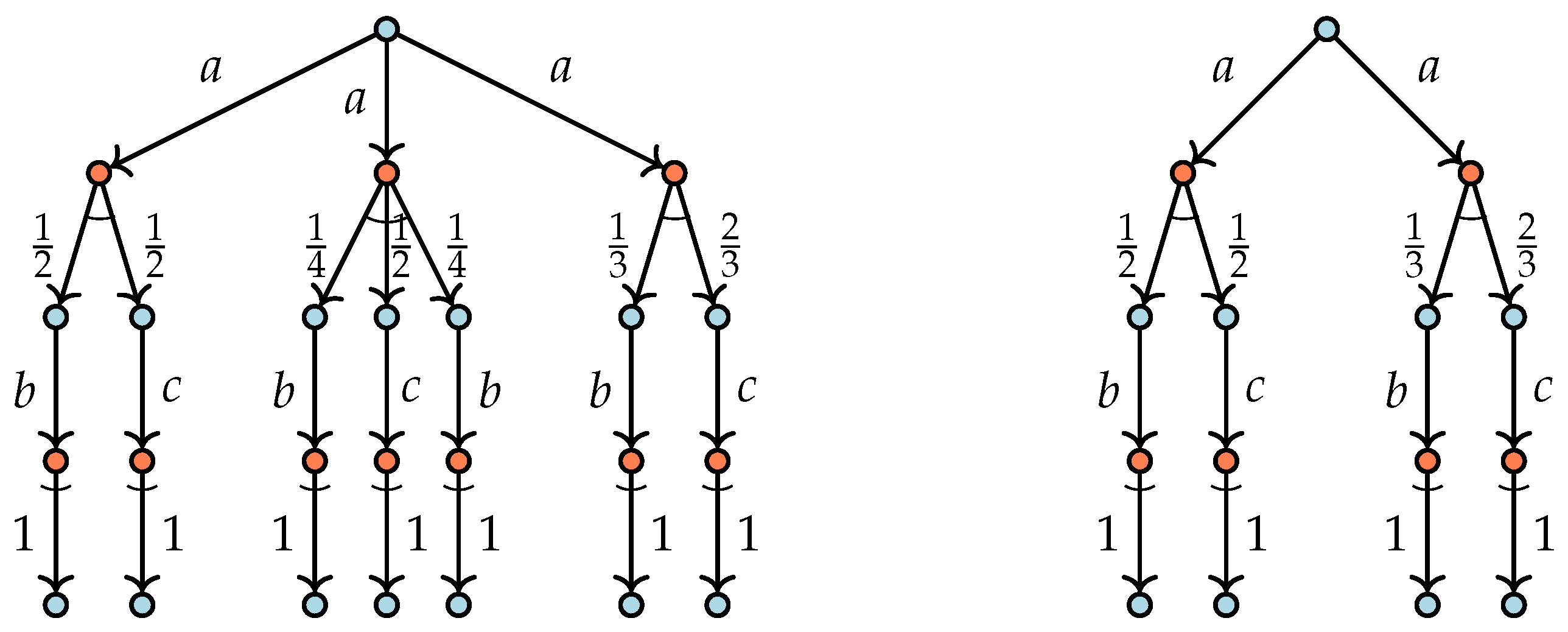
In [1], Larsen and Skou proposed the notion of probabilistic bisimulation. Although described for deterministic transition systems, the same notion is also very suitable for probabilistic transition systems with nondeterminism [2,3], i.e. so-called PLTSs. It expresses that two states are equivalent exactly when the following condition holds: if one state can perform an action ending up in a set of states, each with a certain probability, and then the other state can do the same step ending up in an equivalent set of states with the same distribution of probabilities. Two characteristic nondeterministic transition systems of which the initial states are probabilistically bisimilar are given in Figure 1.

In [4], Baier et al. gave an algorithm for probabilistic bisimulation for PLTSs, thus dealing both with probabilistic and nondeterministic choice, of time complexity $\mathit{O}\left(mn(logm+logn)\right)$ and space complexity $\mathit{O}\left(mn\right)$, where n is the number of states and m is the number of transitions (from states to distributions over states; there is no separate measure for the size of the distributions). As far as we know, it is the only practical algorithm for bisimulation à la Larsen-Skou for PLTSs. In essence, other algorithms for probabilistic systems typically target Markov chains without nondeterminism. The algorithm in [4] performs an iterative refinement of a partition of states and a partition of transitions per action label. The crucial point is splitting the groups of states based on probabilities. For this, a specific data structure is used, called augmented ordered balanced trees, to support efficient storage, retrieval and ordering of states indexed by probabilities.

In this paper, we provide a new algorithm for probabilistic bisimulation for PLTSs of time complexity $\mathit{O}\left((m_a+m_p)log{n}_p+m_{p}log{n}_a)\right)$ and space complexity $\mathit{O}\left(m_a+m_p\right)$, where $n_a$ is the number of states, $m_a$ the number of transitions labelled with actions, $n_p$ the number of distributions and $m_p$ the cumulative support of the distributions. Our $n_a$ coincides with the n of Baier et al. We prefer to use $m_a$, $n_p$, and $m_p$ over m as the former support a more refined analysis. A detailed comparison between the algorithms reveals that, if the distributions have a positive probability for all states, the complexities of the algorithms are similar. However, when distributions only touch a limited number of states, as is often the common situation, the implementation of our algorithm outperforms our implementation of the algorithm in [4], both in time as well as in space complexity.

Similar to the algorithm of Baier et al., our algorithm keeps track of a partition of states and of distributions (referred to as action states and probabilistic states below) but in line with the classical Paige–Tarjan approach [5] it also maintains a courser partition of so-called constellations. The treatment of distributions in our algorithm is strongly inspired by the work for Markov Chain lumping by Valmari and Franceschinis, but our algorithm applies to the richer setting of non-deterministic labelled probabilistic transition systems. Using a brilliant, yet simple argument, taken from [6], the number of times a probabilistic transition is sorted can be limited by the fan-out of the source state of the transition. This leads to the observation that we can use straightforward sorting without the need of any tailored data structure such as augmented ordered balanced trees or similar as in [4,7]. Actually, our algorithm uses a simplification of the algorithm in [6] since the calculation of so-called majority candidates can be avoided, too.

We implemented both the new algorithm and the algorithm from [4]. We spent quite some effort to establish that both implementations are free from programming flaws. To this end, we ran them side-by-side and compared the outcomes on a vast amount of randomly generated probabilistic transition systems (in the order of millions). Furthermore, we took a number of examples from the field, among others from the Prism toolset [8], and ran both implementations on the probabilistic transition systems that were obtained in this way. Time-wise, all benchmarks indicated better results for our algorithm compared to the algorithm from [4]. Even for rather small transition systems of about 100,000 states, performance gains of a factor 10,000 can be achieved. Memory-wise the implementation of our algorithm also outperforms the implementation in [4] when the sizes of the probabilistic state space are larger. Both findings are in line with the theoretical complexity analyses of both algorithms. Both implementations have been incorporated in the open source mCRL2 toolset [9,10].

1.1. Related Work

Probabilistic bisimulation preserves logic equivalence for PCTL [11]. In [12], Katoen c.s. reported up to logarithmic state space reduction obtained by probabilistic bisimulation minimisation for DTMCs. Quotienting modulo probabilistic bisimulation is based on the algorithm in [7]. In the same vein, Dehnert et al. proposed symbolic probabilistic bisimulation minimisation to reduce computation time for model checking PCTL in a setting for DTMCs [13], where an SMT solver is exploited to do the splitting of blocks. Partition reduction modulo probabilistic bisimulation is also used as an ingredient in a counter-example guided abstraction refinement approach (CEGAR) for model checking for PCTL by Lei Song et al. in [14].

For CTMCs, Hillston et al. proposed the notion of contextual lumpability based on lumpable bisimulation in [15]. Their reduction technique uses the Valmari–Franceschinis algorithm for Markov chain lumping mentioned earlier. Crafa and Renzato [16] characterised probabilistic bisimulation of PLTSs as a partition shell in the setting of abstract interpretation. The algorithm for probabilistic bisimulation that comes with such a characterisation turns out to coincide with that in [4]. A similar result applies to the coalgebraic approach to partition refinement in [17] that yields a general bisimulation decision procedure, which can be instantiated with probabilistic system types.

Probabilistic simulation for PLTSs has been treated in [4], too. In [18], maximum flow techniques are proposed to improve the complexity. Zhang and Jansen [19] presented a space-efficient algorithm based on partition refinement for simulation between probabilistic automata, which improves upon the algorithm for simulation by Crafa and Renzato  [16] for concrete experiments taken from the PRISM benchmark suite. A polynomial algorithm, essentially cubic, for deciding weak and branching probabilistic bisimulation by Turrini and Hermanns, recasting the algorithm in [20], is presented in [21].

1.2. Synopsis

The structure of this article is as follows. In Section 2, we provide the notions of a probabilistic transition system as well as that of probabilistic bisimulation. In Section 3, the outline of our algorithm is provided and it is proven that it correctly calculates probabilistic bisimulation. This section ends with an elaborate example. In Section 4 we provide a detailed version the algorithm with a focus on the implementation details necessary to achieve the complexity. In Section 5, we provide some benchmarking results and a few concluding remarks are made in Section 6.

2. Preliminaries

Let S be a finite set. A distribution f over S is a function $f:S\to [0,1]$ such that ${\sum }_{s\in S}f\left(s\right)=1$. For each distribution f, its support is the set $\{s\in S\mid f(s)>0\}$. The size of f is defined as the number of elements in its support, written as $\left|f\right|$. The set of all distributions over a set S is denoted by $\mathcal{D}\left(S\right)$. Distributions are lifted to act on subsets $T\subseteq S$ by $f\left[T\right]={\sum }_{s\in T}f\left(s\right)$.

For an equivalence relation R on S, we use $S/R$ to denote the set of equivalence classes of R. We define $s/R=\{t\in S\mid sRt\}$ and, for a subset T of S, we define $T/R=\{s\in S\mid \exists t\in T:sRt\}$. A partition $\pi =\{B_i\subseteq S\mid i\in I\}$ is a set of non-empty subsets such that $B_i\cap B_j=\varnothing$ for all $i,j\in I$ and ${\bigcup }_{i\in I}{B}_i=S$. Each $B_i$ is called a block of the partition. Slightly ambiguously, we use $S/R$ to denote the set of equivalence classes of R with respect to S. Clearly, the set of equivalence classes of R forms a partition of S. Reversely, a partition $\pi$ of S induces an equivalence relation $R_{\pi }$ on S, by $s{R}_{\pi }t$ iff $s,t\in B$ for some block B of $\pi$. A partition $\pi$ is called a refinement of a partition $\varrho$ iff each block of $\pi$ is a subset of a block of $\varrho$. Hence, each block in $\varrho$ is a disjoint union of blocks from $\pi$.

We use probabilistic labeled transition systems as the canonical way to represent the behaviour of systems.

Definition 1. (Probabilistic Labeled Transition System).

A probabilistic labeled transition system (PLTS) for a set of actions $\mathit{Act}$ is a pair $\mathcal{A}=(S,\stackrel{}{\to })$ where

• S is a finite set of states, and
• $\stackrel{}{\to }\subseteq S\times \mathit{Act}\times \mathcal{D}\left(S\right)$ is a finite transition relation relating states and actions to distributions.

It is common to write $s\stackrel{a}{\to }f$ for $\langle s,a,f\rangle \in \stackrel{}{\to }$. For $s\in S$, $a\in \mathit{Act}$, and a set $F\subseteq \mathcal{D}\left(S\right)$ of distributions, we write $s\stackrel{a}{\to }F$ if $s\stackrel{a}{\to }f$ for some $f\in F$. Similarly, we write $\stackrel{a}{\nrightarrow }F$ if there is no distribution $f\in F$ such that $s\stackrel{a}{\to }f$. For the presentation below, we associate a so-called probabilistic state $u_f$ with each distribution f provided there is some transition $s\stackrel{a}{\to }f$ of $\mathcal{A}$. We write U for $\{u_f\mid \exists s\in S,a\in \mathit{Act}:s\stackrel{a}{\to }f\}$, with typical element u. Note that, since $\stackrel{}{\to }$ is finite, U is also finite. We also use the notation $s\stackrel{a}{\to }{u}_f$ if $s\stackrel{a}{\to }f$ for some $f\in \mathcal{D}\left(S\right)$. As a matter of notation, we write $u_f\left[T\right]$ for $f\left[T\right]$ if probabilistic state $u_f$ corresponds to the distribution f. We sometimes use a so-called probabilistic transition $u_f{\mapsto }_{p}s$ for $0<p⩽1$ and $s\in S$ iff $u_f\left(s\right)=p$. To stress $S\cap U=\varnothing$, we refer to states $s\in S$ as action states.

Below, in particular in the complexity analysis, we use $n_a=\left|S\right|$ as the number of action states, $n_p=\left|U\right|$ as the number of probabilistic states, $m_a=|\to |$ as the number of action transitions and $m_p={\sum }_{u_f\in U}\left|f\right|$ as the cumulative size of the support of the distributions corresponding to all probabilistic states. Note that $m_p⩾n_p$ as every distribution has support of at least size 1.

The following definition for probabilistic bisimulation stems from [1].

Definition 2. (Probabilistic Bisimulation).

Consider a PLTS $\mathcal{A}=(S,\stackrel{}{\to })$. An equivalence relation $R\subseteq S\times S$ is called aprobabilistic bisimulationfor $\mathcal{A}$ iff for all states $s,t\in S$ such that $sRt$ and $s\stackrel{a}{\to }f$, for some action $a\in \mathit{Act}$ and distribution $f\in \mathcal{D}\left(S\right)$, it holds that $t\stackrel{a}{\to }g$ for some distribution $g\in \mathcal{D}\left(S\right)$, and $f\left[B\right]=g\left[B\right]$ for each $B\in S/R$.

Two states $s,t\in S$ are probabilistically bisimilar iff a probabilistic bisimulation R for $\mathcal{A}$ exists such that $sRt$, which we write as $s{\simeq }_{p}t$. Two distributions $f,g\in \mathcal{D}\left(S\right)$, and similarly two probabilistic states $u_f,u_g\in U$, areprobabilistically bisimilariff for all $B\in S/{\simeq }_p$ it holds that $f\left[B\right]=g\left[B\right]$, which we also denote by $f{\simeq }_{p}g$ and $u_f{\simeq }_p{u}_g$, respectively.

By definition, probabilistic bisimilarity is the union of all probabilistic bisimulations. To be able to speak of probabilistically bisimilar distributions (or of probabilistically bisimilar probabilistic states), probabilistic bisimilarity needs to be an equivalence relation. In fact, probabilistic bisimilarity is a probabilistic bisimulation. See [22] for a proof.

3. A Partition Refinement Algorithm for Probabilistic Bisimulation (Outline)

Many efficient algorithms for standard bisimulation calculate partitions of states [5,23,24]. Here, we consider the construction of a partition $\mathcal{B}$ of the sets of action states S and of probabilistic states U for some fixed PLTS $\mathcal{A}$ over a set of actions $\mathit{Act}$. Below blocks of the partition always contain either action states or probabilistic states.

3.1. Stability of Blocks and Partitions

An important notion underlying the algorithm introduced below is that of the stability of a block of a partition. If a block is not stable, it contains states that are not bisimilar. These states either have different transitions or different distributions. We first define the notion of stability more generically on sets instead of on blocks. Then, we lift it to partitions.

Definition 3. (Stable Sets and Partitions).

1. 

A set of action states $B\subseteq S$ is called stable under a set of probabilistic states $C\subseteq U$ with respect to an action $a\in \mathit{Act}$ iff $s\stackrel{a}{\to }C$ whenever $t\stackrel{a}{\to }C$ and vice versa for all $s,t\in B$. The set B is called stable under C iff B is stable under C with respect to all actions $a\in \mathit{Act}$.

2. 

A set of probabilistic states $B\subseteq U$ is called stable under a set of action states $C\subseteq S$ iff $u\left[C\right]=v\left[C\right]$ for all $u,v\in B$.

3. 

A set of states B with $B\subseteq S$, respectively $B\subseteq U$, is called stable under a partition $\mathcal{C}$ of $S\cup U$, with $C\subseteq S$ or $C\subseteq U$ for all $C\in \mathcal{C}$, iff B is stable under each $C\in \mathcal{C}$ with $C\subseteq U$, respectively $C\subseteq S$.

4. 

A partition $\mathcal{B}$ is called stable under a partition $\mathcal{C}$ iff all blocks B of $\mathcal{B}$ are stable under $\mathcal{C}$.

There are two simple but important properties stating that stability is preserved when splitting sets. The first one says that subsets of stable sets are also stable.

Lemma 1.

Let $B\subseteq S$ be a set of action states and $C\subseteq U$ a set of probabilistic states. If B is stable under C, then any $B^{\prime }\subseteq B$ is also stable under C. Similarly, if C is stable under B, then any $C^{\prime }\subseteq C$ is also stable under B.

Proof. 

We only prove the first part as the argument for the second part is essentially the same. If $s,t\in B^{\prime }$, then also $s,t\in B$. As B is stable under C, it holds that for every action $a\in \mathit{Act}$ either both satisfy $s\stackrel{a}{\to }C$ and $t\stackrel{a}{\to }C$, or neither does. Thus, $B^{\prime }$ is stable under C. ☐

The second property says that splitting a set in two parts can only influence the stability of an other set if there is a transition or a positive probability from this other set to one of the parts of the split set.

Lemma 2.

Let $B\subseteq S$ be a set of action states and $C\subseteq U$ a set of probabilistic states.

1. 

Suppose B is stable under C with respect to an action a, $C^{\prime }\subseteq C$, and there is no $s\in B$ such that $s\stackrel{a}{\to }{C}^{\prime }$. Then, B is stable under $C^{\prime }$ and $C\setminus C^{\prime }$ with respect to a.

2. 

Suppose C is stable under B, $B^{\prime }\subseteq B$, and $u\left[B^{\prime }\right]=0$ for all $u\in C$. Then, C is stable under $B^{\prime }$ and $B\setminus B^{\prime }$.

Proof. 

We only provide the proof for the first part of this lemma. If $s,t\in B$, then both $s\stackrel{a}{\nrightarrow }{C}^{\prime }$ and $t\stackrel{a}{\nrightarrow }{C}^{\prime }$ by assumption. Thus, B is stable under $C^{\prime }$ with respect to a. Furthermore, B is stable under $C\setminus C^{\prime }$: Suppose $s,t\in B$ and $s\stackrel{a}{\to }C\setminus C^{\prime }$. Thus, $s\stackrel{a}{\to }C$. As B is stable under C, $t\stackrel{a}{\to }C$, and by assumption $t\stackrel{a}{\nrightarrow }{C}^{\prime }$. Therefore, $t\stackrel{a}{\to }C\setminus C^{\prime }$. Suppose $s\stackrel{a}{\nrightarrow }C\setminus C^{\prime }$. Then, also $s\stackrel{a}{\nrightarrow }C$. As B is stable under C, $t\stackrel{a}{\nrightarrow }C$ and hence, $t\stackrel{a}{\nrightarrow }C\setminus C^{\prime }$. ☐

The following property, called the stability property, says that a partition stable under itself induces a probabilistic bisimulation. In general, partition based algorithms for bisimulation search for such a stable partition.

Lemma 3. Stability Property.

Let $\mathcal{A}=(S,\stackrel{}{\to })$ be a PLTS. If a partition $\mathcal{B}$ for $\mathcal{A}$ is stable under itself, then the corresponding equivalence relation $\mathcal{B}$ on S is a probabilistic bisimulation.

Proof. 

By the first condition of Definition 3 and stability of all blocks in $\mathcal{B}$ we have that either $B\subseteq S$ or $B\subseteq U$, for each block $B\in \mathcal{B}$. We write $s\mathcal{B}t$ iff $s,t\in B$ for some $B\in \mathcal{B}$. Note that used in this way $\mathcal{B}$ is an equivalence relation on S.

Suppose $s\mathcal{B}t$ for some $s,t\in S$ and $s\stackrel{a}{\to }f$. Let $u\in U$ correspond to f. Say $s,t\in B$ and $u\in B^{\prime }$ for some blocks $B,B^{\prime }\in \mathcal{B}$. Then, $s\stackrel{a}{\to }{B}^{\prime }$. By stability of B for $B^{\prime }$, it follows that $t\stackrel{a}{\to }{B}^{\prime }$. Hence, $v\in B^{\prime }$ and $g\in \mathcal{D}\left(S\right)$ exist such that v corresponds to g and $s\stackrel{a}{\to }g$. Therefore, for any block $B^{\prime \prime }\in \mathcal{B}$ we have $f\left[B^{\prime \prime }\right]=u\left[B^{\prime \prime }\right]=v\left[B^{\prime \prime }\right]=g\left[B^{\prime \prime }\right]$ since the block $B^{\prime }$ of u and v is stable under each block $B^{\prime \prime }$ of $\mathcal{B}$.

Thus, the stable partition $\mathcal{B}$ induces an equivalence relation that satisfies the conditions for a probabilistic bisimulation of Definition 2, as was to be shown. ☐

3.2. Outline of the Algorithm

We present our algorithm in two stages. An abstract description of the algorithm is presented as Algorithm 1; the detailed algorithm is provided as Algorithm 2. The set-up of Algorithm 1 is a fairly standard, iterative refinement of a partition $\mathcal{B}$, in this particular case containing both action states and probabilistic states, which are treated differently. In addition, following the approach of Paige and Tarjan [5], we maintain a coarser partition $\mathcal{C}$, which we call the set of constellations. Each constellation in partition $\mathcal{C}$ is a union of one or more blocks of $\mathcal{B}$, thus $\mathcal{B}$ is a refinement of $\mathcal{C}$. A constellation $C\in \mathcal{C}$ that consists of exactly one block in $\mathcal{B}$ is called trivial. We refine partitions $\mathcal{B}$ and $\mathcal{C}$ until $\mathcal{C}$ only contains trivial constellations (see Line 5 of Algorithm 1).

Algorithm 1 Abstract Partition Refinement Algorithm for Probabilistic Bisimulation.

1: functionpartition-refinement 2: $\mathcal{C}:=\{S,U\}$ 3: $\mathcal{B}:=\left\{U\right\}\cup \{S_A\mid A\subseteq \mathit{Act}\}$ 4:       where $S_A=\{s\in S\mid \forall a\in A\exists u\in U:s\stackrel{a}{\to }u\}$ 5: while$\mathcal{C}$ contains a non-trivial constellation C do 6:  choose block $B_C$ from $\mathcal{B}$ in C 7:  replace in $\mathcal{C}$ constellation C by $B_C$ and $C\setminus B_C$ 8:  if C contains probabilistic states then 9:   for all blocks B of action states in $\mathcal{B}$ unstable under $B_C$ or $C\setminus B_C$ do 10:    refine $\mathcal{B}$ by splitting B into blocks of states with the same actions into $B_C$ and $C\setminus B_C$ 11:   end for 12:  else 13:   for all blocks B of probabilistic states in $\mathcal{B}$ unstable under $B_C$ do 14:    refine $\mathcal{B}$ by splitting B into blocks of states with equal probabilities into $B_C$ 15:   end for 16:  end if 17: end while 18: return$\mathcal{B}$

Algorithm 2 Partition Refinement Algorithm for Probabilistic Bisimulation

Among others, we preserve the invariant that the blocks in partition $\mathcal{B}$ are always stable under partition $\mathcal{C}$. If all constellations in $\mathcal{C}$ are trivial, then the partitions $\mathcal{B}$ and $\mathcal{C}$ coincide. Hence, the blocks in $\mathcal{B}$ are stable under itself, and according to Lemma 3 we have found a probabilistic bisimulation. Our algorithm works by iteratively refining the set of constellations $\mathcal{C}$. When refining $\mathcal{C}$, we must also refine $\mathcal{B}$ to preserve the above mentioned invariant.

Since the set of states of a PLTS is finite (cf. Definition 1) refinement of the partitions $\mathcal{B}$ and $\mathcal{C}$ cannot be repeated indefinitely. Thus, termination of the algorithm is guaranteed. The partition consisting of singletons of action states and of probabilistic states is the finest that can be obtained, but this is only possible if all states are not bisimilar. In practice, the main loop of the algorithm stops well before reaching that point.

The algorithm maintains the following three invariants:

Invariant 1.

Probabilistic bisimilarity ${\simeq }_p$ is a refinement of $\mathcal{B}$.

Invariant 2.

Partition $\mathcal{B}$ is a refinement of partition $\mathcal{C}$.

Invariant 3.

Partition $\mathcal{B}$ is stable under the set of constellations $\mathcal{C}$ (mentioned already above).

Invariant 1 states that if two action states or two probabilistic states are probabilistically bisimilar, then they are in the same block of partition $\mathcal{B}$. Thus, the partition-refinement algorithm will not separate states if they are bisimilar. By Invariant 2, we have that, at the end and at the start of each iteration, each constellation in $\mathcal{C}$ is a union of blocks in $\mathcal{B}$. Invariant 3 says that blocks in partition $\mathcal{B}$ cannot be split by blocks in constellation $\mathcal{C}$.

In Lines 2 and 3 of Algorithm 1, the set of constellation and the initial partition are set such that the invariants hold. All probabilistic states are put in one block, and all action states with exactly the same actions labelling outgoing transitions are also put together in blocks. (Note the universal quantification over all actions a in A for the set comprehension at Line 4 to ensure that only maximal blocks are included in $\mathcal{B}$ for it being a partition indeed.) The set of constellations contains two constellations namely one with all action states, and one with all probabilistic states. It is straightforward to see that Invariants 1 and 2 hold. Invariant 3 is valid because all transitions from action states go to probabilistic states and vice versa.

Invariants 1–3 guarantee correctness of Algorithm 1. That is, from the invariants, it follows that, upon termination, when all constellations have become trivial, the computed partition $\mathcal{B}$ identifies probabilistically bisimilar action states and probabilistically bisimilar probabilistic states.

Theorem 1.

Consider the partition $\mathcal{B}$ resulting from Algorithm 1. We find that (i) two action states are in the same block of $\mathcal{B}$ iff they are probabilistically bisimilar, and (ii) two probabilistic states are in the same block of $\mathcal{B}$ iff they are probabilistically bisimilar.

Proof. 

Upon termination, because of the while loop of Algorithm 1, all constellations of $\mathcal{C}$ are trivial, i.e. each constellation in $\mathcal{C}$ consists of exactly one block of $\mathcal{B}$. Hence, by Invariant 2, the partitions $\mathcal{B}$ and $\mathcal{C}$ coincide. Thus, by Invariant 3, each block of $\mathcal{B}$ is stable under each block in $\mathcal{B}$. In other words, partition $\mathcal{B}$ is stable under itself.

By the Stability Property of Lemma 3, we have that $\mathcal{B}$ is a probabilistic bisimulation on S. It follows that two action states in the same block of $\mathcal{B}$ are probabilistically bisimilar. Reversely, by Invariant 1, probabilistically bisimilar action states are in the same block of $\mathcal{B}$. Thus, ${\simeq }_p$ and $\mathcal{B}$ coincide on S. In other words, two action states are in the same block of $\mathcal{B}$ iff they are probabilistically bisimilar.

To compare ${\simeq }_p$ and the relation $\mathcal{B}$ on U, choose probabilistic states $u,v\in U$ such that $u\mathcal{B}v$. Thus, u and v are in the same block of $\mathcal{B}$. By stability of block B for $\mathcal{B}$ it follows that $u\left[B^{\prime }\right]=v\left[B^{\prime }\right]$, for each block $B^{\prime }\subseteq S$. Since ${\simeq }_p$ and $\mathcal{B}$ coincide on S this implies $u\left[B^{\prime }\right]=v\left[B^{\prime }\right]$ for all $B^{\prime }\in S/{\simeq }_p$. Thus, we have $u{\simeq }_{p}v$. Reversely, if $u{\simeq }_{p}v$, we have $u,v\in B$ for some block B of $\mathcal{B}$ by Invariant 1. Thus, two probabilistic states are in the same block of $\mathcal{B}$ iff they are probabilistically bisimilar. ☐

It is worth noting that in Line 5 of Algorithm 1 an arbitrary non-trivial constellation is chosen and in Line 6 an arbitrary block $B_C$ is selected from C (we later put a constraint on the choice of $B_C$). In general, there are many possible choices and this influences the way the final partition is calculated. The previous theorem indicates that the final partition is not affected by this choice, neither is the complexity upper-bound, see Section 4.6. However, it is conceivable that practical runtimes can be improved by choosing the non-trivial constellation C and the block $B_C$ optimally.

3.3. Refining the Set of Constellations and Restoring the Invariants

As we see from the high-level description of the partition refinement Algorithm 1, a non-trivial constellation C and a constituent block $B_C$ are chosen (Lines 5 and 6) and C is replaced in $\mathcal{C}$ by the smaller constellations $B_C$ and $C\setminus B_C$ (Line 7). This preserves Invariants 1 and 2, but Invariant 3 may be violated as stability under $B_C$ or $C\setminus B_C$ (or both) may be lost: On the one hand, it may be the case that two actions states s and t both have an a-transition into C, but s may have one to $B_C$ but t to $C\setminus B_C$ only or vice versa. On the other hand, it may be the case that two probabilistic states u and v yield the same value for C as a whole, i.e. $u\left[C\right]=v\left[C\right]$, but by no means this needs to hold for $B_C$ or $C\setminus B_C$, i.e. $u\left[B_C\right]\ne v\left[B_C\right]$ and $u[C\setminus B_C]\ne v[C\setminus B_C]$. Therefore, in the remainder of the body of Algorithm 1, the blocks that are unstable under $B_C$ and $C\setminus B_C$ are split such that Invariant 3 is restored, both for blocks of actions states (Lines 9 and 10) and for blocks of probabilistic states (Lines 13 and 14). In the next section, the detailed Algorithm 2 describes how this is done precisely.

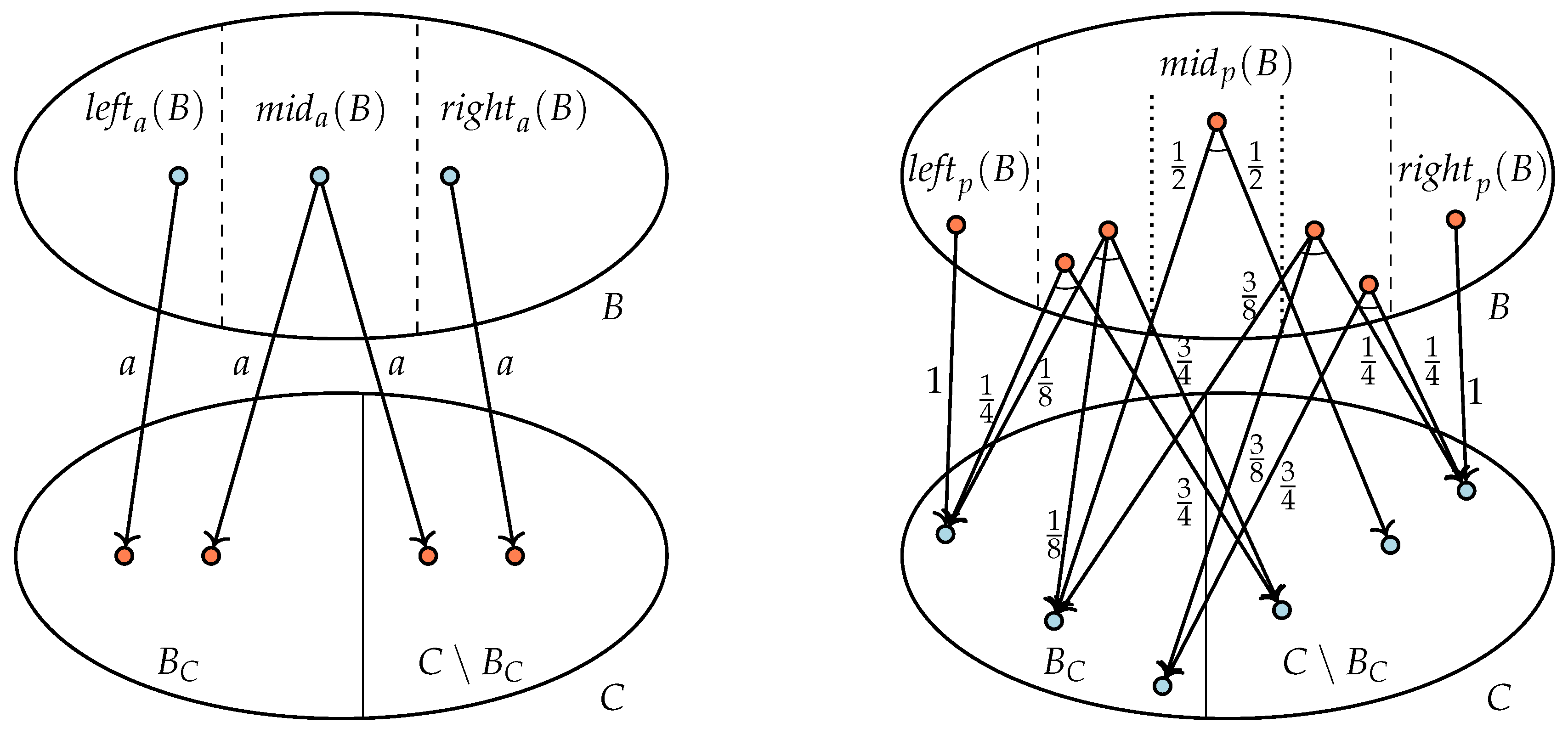
The general situation when splitting a block B for a constellation C containing a block $B_C$ is depicted in Figure 2, at the left where B contains action states and at the right where B consists of probabilistic states. We first consider the case at the left.

In this case, block $B\subseteq S$ is stable under constellation $C\subseteq U$ and C is non-trivial. Thus, C properly contains a block $B_C$ of $\mathcal{B}$, and we distinguish two non-empty subsets of C, the block $B_C$ on its own and the remaining blocks together in $C\setminus B_C$. As B is stable under C, the block B can only be unstable under $B_C$ or $C\setminus B_C$ if there is an action $a\in \mathit{Act}$ and a state $s\in B$ such that $s\stackrel{a}{\to }{B}_C$ (Lemma 2.1). Thus, we only investigate and split blocks, for which such a transition $s\stackrel{a}{\to }{B}_C$ exists.

We can restore stability by splitting B into the following three subsets:

$$\begin{array}{ccc}\hfill {\mathit{left}}_a\left(B\right)& =& \{s\in B\mid s\stackrel{a}{\to }{B}_C\wedge s\stackrel{a}{\nrightarrow }C\setminus B_C\},\hfill \\ \hfill {\mathit{mid}}_a\left(B\right)& =& \{s\in B\mid s\stackrel{a}{\to }{B}_C\wedge s\stackrel{a}{\to }C\setminus B_C\},\mathrm{and}\hfill \\ \hfill {\mathit{right}}_a\left(B\right)& =& \{s\in B\mid s\stackrel{a}{\nrightarrow }{B}_C\wedge s\stackrel{a}{\to }C\setminus B_C\}.\hfill \end{array}$$

Note that the remaining set $\{s\in B\mid s\stackrel{a}{\nrightarrow }{B}_C\wedge s\stackrel{a}{\nrightarrow }C\setminus B_C\}$ must be empty; if not, this would imply that there is some action state t such that $t\stackrel{a}{\nrightarrow }C$. However, due to the existence of state s such that $s\stackrel{a}{\to }{B}_C$, this would mean that block B is unstable under C, contradicting Invariant 3.

Checking that the sets ${\mathit{left}}_a\left(B\right)$, ${\mathit{mid}}_a\left(B\right)$, ${\mathit{right}}_a\left(B\right)$ are stable under C is immediate. As subsets of stable sets are also stable (Lemma 1) and B is stable all other configurations of $\mathcal{C}$, the sets ${\mathit{left}}_a\left(B\right)$, ${\mathit{mid}}_a\left(B\right)$, and ${\mathit{right}}_a\left(B\right)$ are stable under all other configurations of $\mathcal{C}$ too.

Note that, due to the existence of state s with $s\stackrel{a}{\to }{B}_C$, it is not possible that both ${\mathit{left}}_a\left(B\right)$ and ${\mathit{mid}}_a\left(B\right)$ are equal to the empty set. It is however possible that ${\mathit{left}}_a\left(B\right)=B$ or ${\mathit{mid}}_a\left(B\right)=B$, leaving the other two sets empty.

Lines 9 and 10 can now be read as follows. For all $a\in \mathit{Act}$, investigate all blocks B such that there is an action state $s\in B$ with $s\stackrel{a}{\to }{B}_C$ as these blocks are the only candidates to be unstable. Replace each such block B in $\mathcal{B}$ by $\{{\mathit{left}}_a\left(B\right),{\mathit{mid}}_a\left(B\right),{\mathit{right}}_a\left(B\right)\}\setminus \varnothing$ to restore stability under $B_C$ and $C\setminus B_C$.

Invariants 1 and 2 are preserved by splitting B. For Invariant 2, this is trivial by construction. For Invariant 1, note that the states in different blocks among ${\mathit{left}}_a\left(B\right),{\mathit{mid}}_a\left(B\right),{\mathit{right}}_a\left(B\right)$ cannot be probabilistically bisimilar as they have unique transitions to states $B_C$ and $C\setminus B_C$ and these target states cannot be bisimilar by Invariant 1. Thus, if two states of B are probabilistically bisimilar then both are in the same subset ${\mathit{left}}_a\left(B\right)$, ${\mathit{mid}}_a\left(B\right)$, or ${\mathit{right}}_a\left(B\right)$ of B.

We next turn to the case of a set of probabilistic states B, see the right-side of Figure 2. Again, we assume that the non-trivial constellation C is replaced by its two non-empty subsets $B_C$ and $C\setminus B_C$. As in the previous case, although the block B is stable under the constellation C, this may not be the case under the subsets $B_C$ and $C\setminus B_C$.

To restore stability, we now consider for all q, $0⩽q⩽1$, the sets

$$\begin{array}{ccc}\hfill B_q& =& \{u\in B\mid u\left[B_C\right]=q\}.\hfill \end{array}$$

Note that, for finitely many $q\in [0,1]$, we have $B_q\ne \varnothing$. Observe that each set $B_q$ is stable under $B_C$ as by construction $u\left[B_C\right]=v\left[B_C\right]=q$ for any $u,v\in B_q$. The set $B_q$ is also stable under $C\setminus B_C$. To see this consider two states $u,v\in B_q$. As block $B\subseteq U$ is stable under constellation $C\subseteq S$, $u\left[C\right]=v\left[C\right]$. Hence, $u[C\setminus B_C]=u\left[C\right]-u\left[B_C\right]=v\left[C\right]-v\left[B_C\right]=v[C\setminus B_C]$. By Lemma 1, the new blocks $B_q$ are also stable under the other constellations in $\mathcal{C}$.

According to Lemma 2.2, only those blocks B that contain a probabilistic state $u\in B$ such that $u\left[B_C\right]>0$ can be unstable under $B_C$ and $C\setminus B_C$. Thus, at Line 13 of Algorithm 1 we consider all those blocks B and replace each of them by the non-empty subsets $B_q$, $0⩽q⩽1$ at Line 14 in $\mathcal{B}$. This makes the partition stable again under all constellations in $\mathcal{C}$, in particular under the new constellations $B_C$ and $C\setminus B_C$.

Again, it is straightforward to see that Invariants 1 and 2 are not violated by replacing the block B by the blocks $B_q$. For Invariant 1, if states are probabilistically bisimilar in B, they remain in the same block $B_q$. For Invariant 2, as B is refined, partition $\mathcal{B}$ remains a refinement of partition $\mathcal{C}$.

For the detailed algorithm in Section 4, it is required to group the sets $B_q$ as follows: ${\mathit{left}}_p\left(B\right):=B_0$, ${\mathit{right}}_p\left(B\right):=B_1$, and ${\mathit{mid}}_p\left(B\right)=\{B_q\mid 0<q<1\}$. This does not play a role here, but ${\mathit{left}}_p\left(B\right)$, ${\mathit{mid}}_p\left(B\right)$, and ${\mathit{right}}_p\left(B\right)$ are already indicated in Figure 2, in particular ${\mathit{mid}}_p\left(B\right)=\{B_{\frac{1}{4}},B_{\frac{1}{2}},B_{\frac{3}{4}}\}$.

3.4. An Example

We provide an example to illustrate how Algorithm 1 calculates partitions.

Example 1.

Consider the PLTS given in Figure 3. We provide a detailed account of the partitions that are obtained when calculating probabilistic bisimulation. The obtained partitions are listed in

Table 1. The generated partitions for the PLTS of Example 1.

	Blocks of Actions States		Blocks of Probabilistic States
	S0 = {t1, t3, t4, t6, t7, r1–5}		U0 = {u1–6, v1–5}
	S1 = {s1–4}		U1 = {u1, u3, v1–5}
	S2 = {t2, t5, t8, t9}		U2 = {u2, u4}
	S3 = {t10}		U3 = {u5, u6}
	S4 = {s1, s2}		U4 = {u5}
	S5 = {s3, s4}		U5 = {u6}
	S6 = {s3}
	S7 = {s4}
	$\mathcal{B}$		$\mathcal{C}$
0	S0, S1, S2, S3	U0	S0 ∪ S1 ∪ S2 ∪ S3	U0
1	S0, S1, S2, S3	U1, U2, U3	S0, S1 ∪ S2 ∪ S3	U1 ∪ U2 ∪ U3
2	S0, S1, S2, S3	U1, U2, U3	S0, S1, S2 ∪ S3	U1 ∪ U2 ∪ U3
3	S0, S1, S2, S3	U1, U2, U4, U5	S0, S1, S2, S3	U1 ∪ U2 ∪ U4 ∪ U5
4	S0, S2, S3, S4, S5	U1, U2, U4, U5	S0, S2, S3, S4 ∪ S5	U1, U2 ∪ U4 ∪ U5
5	S0, S2, S3, S4, S5	U1, U2, U4, U5	S0, S2, S3, S4 ∪ S5	U1, U2, U4 ∪ U5
6	S0, S2, S3, S4, S6, S7	U1, U2, U4, U5	S0, S2, S3, S4 ∪ S6 ∪ S7	U1, U2, U4, U5
7	S0, S2, S3, S4, S6, S7	U1, U2, U4, U5	S0, S2, S3, S4, S6 ∪ S7	U1, U2, U4, U5
8	S0, S2, S3, S4, S6, S7	U1, U2, U4, U5	S0, S2, S3, S4, S6, S7	U1, U2, U4, U5

. In the lower table, nine partitions together with their constellations are listed that are generated for a run of Algorithm 1. In the upper table the blocks that occur in these partitions are defined. Observe that we put the blocks and constellations with action states and probabilistic states in different columns. This is only for clarity, as in the current partition and the current set of constellations they are joined.

Algorithm 1 starts with four blocks of action states, $S_0$ to $S_3$, which contain the action states with no outgoing transitions and those with an outgoing transition labelled with a, with b, and with c, respectively. In the algorithm, all probabilistic states are initially collected in block $U_0$. There are two constellations, viz. $S_0\cup S_1\cup S_2\cup S_3$ and $U_0$. These initial partitions are listed in R0w 0 of the lower part of Table 1.

Since the constellation with action states is non-trivial we split it, rather arbitrarily, in $S_0$ and $S_1\cup S_2\cup S_3$. The block $U_0$ is not stable under $S_0$ and $S_1\cup S_2\cup S_3$ and is split in $U_1=\left\{u_1,u_3,v_{1-5}\right\}$, $U_2=\left\{u_2,u_4\right\}$ and $U_3=\left\{u_5,u_6\right\}$. This is because we have $u\left[S_0\right]=1$ for u equal to $u_1$, $u_3$, and $v_1$ to $v_5$; we have $u\left[S_0\right]=\frac{1}{2}$ for u equal to $u_2$ and $u_4$; we have $u_5\left[S_0\right]=0$ and $u_6\left[S_0\right]=0$. The resulting partitions are listed at Row 1 in Table 1.

For the second iteration, we consider the non-trivial constellation $S_1\cup S_2\cup S_3$ and split it into $S_1$ and $S_2\cup S_3$. Note, the action states $s_1$ to $s_4$ in $S_1$ do not have incoming transitions. Consequently, for all $u\in U_1$, we have $u\left[S_1\right]=0$; for all $u\in U_2$ we have $u\left[S_1\right]=0$; for all $u\in U_3$ we have $u\left[S_1\right]=0$. Thus, all blocks of probabilistic states are stable under $S_1$ and $S_2\cup S_3$. Hence, no block is split.

In the third iteration, we split the non-trivial constellation $S_2\cup S_3$ into $S_2$ and $S_3$. For all, $u\in U_1$ we have $u\left[S_2\right]=0$. Thus, $U_1$ is stable under $S_2$ and $S_3$. For $U_2$, the probabilistic states $u_2$ and $u_4$ agree on the value $\frac{1}{2}$ for $S_2$, hence for $S_3$ too. Thus, $U_2$ is stable as well. However, for $u_5$ and $u_6$ in $U_3$ we have $u_5\left[S_2\right]=1$ and $u_6\left[S_2\right]=\frac{1}{3}$. Therefore, $U_1$ needs to be split in $U_4=\left\{u_5\right\}$ and $U_5=\left\{u_6\right\}$.

At this point, all constellations with actions states are trivial, so at iteration 4 we turn to the non-trivial constellation of probabilistic states $U_1\cup U_2\cup U_4\cup U_5$ and split it into $U_1$ and $U_2\cup U_4\cup U_5$. Block $S_0$ is stable since each of its states has no transitions at all. Block $S_1$ is not stable: $s_1,s_2\stackrel{a}{\to }{U}_1$ and $s_1,s_2\stackrel{a}{\to }{U}_2\cup U_4\cup U_5$, but $s_3,s_4\stackrel{a}{\nrightarrow }{U}_1$ and $s_3,s_4\stackrel{a}{\to }{U}_2\cup U_4\cup U_5$. Thus, $S_1$ needs to be split into $S_4=\left\{s_1,s_2\right\}$ and $S_5=\left\{s_3,s_4\right\}$. Block $S_2$ is stable since its states have only b-transitions into $U_1$. Block $S_3$ is a singleton and therefore cannot be split.

The following iteration, Iteration 5, sets $U_2$ and $U_4\cup U_5$ apart as constellations. Again, in absence of transitions, block $S_0$ is stable under $U_2$ and $U_4\cup U_5$. The same holds for $S_2$ that has only b-transitions into $U_0$. Block $S_3$ can be ignored. For $S_4$, both $s_1$ and $s_2$ have an a-transition into $U_2$ as their only transition. Hence, block $S_4$ is stable. Similarly, $S_5$ is stable, as its states $s_3$ and $s_4$ both have an a-transition into $U_4\cup U_5$ and no other transitions. Overall, in this iteration, no blocks require splitting to restore Invariant 3.

Next, at Iteration 6, we split non-trivial constellation $U_4\cup U_5$ into $U_4$ and $U_5$. For $S_0$, $S_2$, $S_3$ and $S_4$ we conclude stability in the same way as in the previous iteration. However, now we have for $s_3,s_4\in S_5$ on the one hand $s_3\stackrel{a}{\to }{U}_4$ and $s_3\stackrel{a}{\nrightarrow }{U}_5$, but on the other hand $s_4\stackrel{a}{\nrightarrow }{U}_4$ and $s_4\stackrel{a}{\to }{U}_5$. Hence, $S_5$ needs to be split, yielding the singletons $S_6=\left\{s_3\right\}$ and $S_7=\left\{s_4\right\}$.

Returning to constellations of actions states, at Iteration 7, we split $S_4\cup S_6\cup S_7$ over $S_4$ and $S_6\cup S_7$. All probabilistic states have value 0 for both $S_4$ and $S_6\cup S_7$, hence no split of probabilistic blocks is needed.

This is similar in Iteration 8, where the non-trivial constellation $S_6\cup S_7$ is split, and none of the blocks become unstable. Now, all constellations are trivial and the algorithm terminates. According to the Stability Property, Lemma 3, the corresponding equivalence relation is a probabilistic bisimulation. Thus, the final partition is $\left\{S_0,S_2,S_3,S_4,S_6,S_7,U_1,U_2,U_4,U_5\right\}$. Moreover, the deadlock states $t_1,t_3,t_4,t_6,t_7$ and $r_1$ to $r_5$ are probabilistically bisimilar, the states $t_2,t_5,t_8,t_9$ that have only a b-transition into a Dirac distribution to deadlock are probabilistically bisimilar, the states $s_1$ and $s_2$ are probabilistically bisimilar (which is clear when identifying states $t_7$ and $t_8$), whereas the remaining action states $s_3$, $s_4$ and $t_{10}$ have no probabilistically bisimilar counterpart. For the probabilistic states the states $u_1$, $u_3$ and $v_1$ to $v_5$ are identified by probabilistic bisimulation. This also holds for the probabilistic states $u_2$ and $u_4$. Probabilistic states $u_5$ and $u_6$ each have no probabilistically bisimilar counterpart.

4. A Partition-Refinement Algorithm for Probabilistic Bisimulation (Detailed)

Algorithm 1 gives an outline but leaves many details implicit. The detailed refinement-partition algorithm is presented in this section as Algorithm 2. It has the same structure as Algorithm 1, but in this section we focus on how to efficiently calculate whether and how blocks must be split, and how this split is actually carried out. We first explain grouping of action transitions per action, next we introduce various data structures that are used by the algorithm, subsequently we explain how the algorithm is working line-by-line, and finally we give an account of its complexity.

4.1. Grouping Action Transitions per Action Label

To obtain the complexity bound of our algorithm, it is essential that we can group action transitions by actions linearly in the number of transitions. Grouping means that the action transitions with the same action occur consecutively in this ordering. It is not necessary that the transitions are ordered according to some overall ordering.

We assume that $\left|\mathit{Act}\right|⩽m_a$ and that the actions in $\mathit{Act}$ are consecutively numbered. Recall, $m_a$ denotes the number of transitions $s\stackrel{a}{\to }u$. These assumptions are easily satisfied, by removing those actions in $\mathit{Act}$ that are not used in transitions and by sorting and numbering the remaining action labels. Sorting these actions adds a negligible $O\left(\right|\mathit{Act}|log|\mathit{Act}\left|\right)⩽O(m_{a}log{m}_a)$.

Grouping transitions is performed by an array of buckets indexed with actions. All transitions are put in the appropriate bucket in constant time exploiting actions being numbered. Furthermore, all buckets that contain transitions are linked together. When all transitions are in the buckets, a straightforward traversal of all linked buckets provides the transitions in a grouped order. This requires time linear in the number of considered action transitions. Note that the number of buckets is equal to $\left|\mathit{Act}\right|⩽m_a$ and, therefore, the buckets do not require more than linear memory.

4.2. Data Structures

We give a concise overview of the concrete data structures in the algorithm for states, transitions, blocks, and constellations. We list the names of the fields in these data structures in a programming vein to keep a close link with the actual implementation.

The chosen data structures are not particularly optimised. Exploiting ideas from [6,24,25] to store states, blocks, and constellations, usage of time and memory can be further reduced. All data structures come in two flavours, one related to actions and the other related to probabilities. We treat them simultaneously and only mention their differences when appropriate.

4.2.1. Global

In the detailed algorithm, there are arrays containing transitions, actions, blocks and constellations. There is a stack of non-trivial constellations to identify in constant time which constellation must be investigated in the main loop. Furthermore, there is an array containing the variables $\mathit{state}\_\mathit{to}\_\mathit{constellation}\_\mathit{cnt}$, which are explained below.

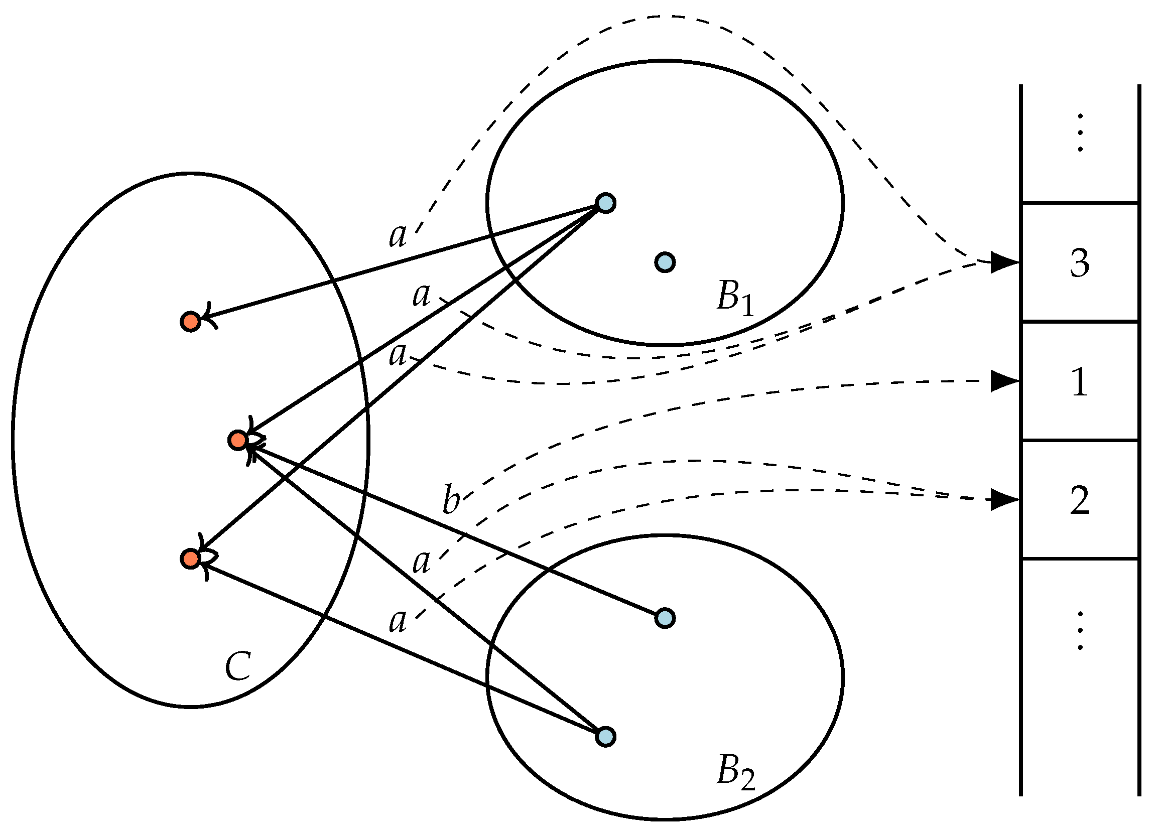
For all action transitions $s\stackrel{a}{\to }u$, it is maintained how many action transitions there are labelled with the same action a, and that go from s to the constellation C containing u. This value is called $\mathit{state}\_\mathit{to}\_\mathit{constellation}\_\mathit{cnt}$ for this transition. The value is required to efficiently split probabilistic blocks (the idea of using such variables stems from [5]). For each state s, constellation C, and action a there is one instance of $\mathit{state}\_\mathit{to}\_\mathit{constellation}\_\mathit{cnt}$ stored in a global array. Each transition $s\stackrel{a}{\to }u$ contains a reference called $\mathit{state}\_\mathit{to}\_\mathit{constellation}\_\mathit{cnt}\_\mathit{ptr}$ to the appropriate value in this array. See Figure 3 for a graphical illustration with a constellation C of probabilistic states and blocks $B_1$ and $B_2$ of action states. The purpose of this construction is that $\mathit{state}\_\mathit{to}\_\mathit{constellation}\_\mathit{cnt}$ can be changed by one operation for all transitions from the same state with the same action to the same constellation, simultaneously.

4.2.2. Transition

Each transition consists of the fields $\mathit{from}$, $\mathit{label}$ and $\mathit{to}$. Here, $\mathit{from}$ and $\mathit{to}$ refer to an action/probabilistic state, and $\mathit{label}$ is the action label or probabilistic label of the transition. The action labels are consecutive numbers; the probabilistic labels are exact fractions. Action transitions also contain a reference $\mathit{state}\_\mathit{to}\_\mathit{constellation}\_\mathit{cnt}\_\mathit{ptr}$ to the variable $\mathit{state}\_\mathit{to}\_\mathit{constellation}\_\mathit{cnt}$ as indicated above.

4.2.3. State

Each action state and probabilistic state contains a list of incoming transitions and a reference to the block in which the state resides. For intermediate calculations, each state contains a boolean $\mathit{mark}\_\mathit{state}$ which is used to indicate that a state has been marked. Each action state also contains two more variables for temporary use. When deciding whether blocks need to be split, the variable $\mathit{residual}\_\mathit{transition}\_\mathit{cnt}$ indicates how many residual transitions there are to blocks $C\setminus B_C$ when splitting takes place by a block $B_C$. The variable $\mathit{transition}\_\mathit{cnt}\_\mathit{ptr}$ is used to let the variable $\mathit{state}\_\mathit{to}\_\mathit{constellation}\_\mathit{cnt}\_\mathit{ptr}$ for an action transition point to a new instance of $\mathit{state}\_\mathit{to}\_\mathit{constellation}\_\mathit{cnt}$ when this transitions is moved to a new block. In probabilistic states, there is the temporary variable $\mathit{cumulative}\_\mathit{prob}$ used to calculate the total probability to reach a block under splitting.

4.2.4. Block

Blocks contain an indication of the constellation in which it occurs, a list of the states contained in the block including the size of this list, and a list of transitions ending in this block. For blocks of action states, this list of transitions is grouped by action label, i.e., transitions with the same action label are a consecutive sublist. For temporary use, there is also a variable to indicate that the block is marked. This marking contains exactly the information that the functions $\mathit{aMark}$ and $\mathit{pMark}$, discussed below, provide for blocks of action states and blocks of probabilistic states, respectively.

4.2.5. Constellation

Finally, constellations contain a list of the blocks in the constellation as well as the cumulative number of states contained in all blocks in this constellation.

4.3. Explanation of the Detailed Algorithm

Algorithm 1 focuses on how, by refining partitions and sets of constellations, probabilistic bisimulation can be calculated. In Algorithm 2, we stress the details of carrying out concrete refinement steps to realise the required time bound. As already indicated, the overall structure of both algorithms is the same.

The initial Lines 2 and 3 of Algorithm 2 are the same as those of Algorithm 1. In Line 3, the partition $\mathcal{B}$ is set to contain one block with all probabilistic states and a number of blocks of action states, grouped per common outgoing action labels. Thus, two action states are in the same block initially if their menu, i.e., the set of actions for which there is a transition, is identical. This initial partition $\mathcal{B}$ is calculated using a simple partition refinement algorithm on outgoing transitions of states. This operation is linear in the number of outgoing action transitions when using grouping of transitions as explained in Section 4.1.

At Line 4, the incoming transitions are ordered on actions as indicated in Section 4.1. At Line 5, an array with one instance of $\mathit{state}\_\mathit{to}\_\mathit{constellation}\_\mathit{cnt}$ for each action label is made where each instance contains the number of action transitions that contain that action label. The reference $\mathit{state}\_\mathit{to}\_\mathit{constellation}\_\mathit{cnt}$ for each action transition is set to refer to the appropriate instance in this array. This is done by simply traversing all transitions $s\stackrel{a}{\to }u$ grouped by action labels and incrementing the appropriate entry in the array containing all $\mathit{state}\_\mathit{to}\_\mathit{constellation}\_\mathit{cnt}$ variables. The appropriate entry can be found using the temporary variable $\mathit{transition}\_\mathit{cnt}\_\mathit{ptr}$ associated to state s. If no entry for $\mathit{state}\_\mathit{to}\_\mathit{constellation}\_\mathit{cnt}$ exists yet, the variable $\mathit{transition}\_\mathit{cnt}\_\mathit{ptr}$ belonging to s is null and an appropriate entry must be created.

In Line 6, selecting a non-trivial constellation is straightforward, as a stack of non-trivial constellations is maintained. Initially, this stack contains $\mathcal{C}=\{\mathcal{S},\mathcal{U}\}$. To obtain the required time complexity, we select $B_C$ such that $|B_C|⩽\frac{1}{2}\left|C\right|$ in Line 8. This is done in constant time as we know the number of states in C. Hence, either the first or second block B of constellation C satisfies that $\left|B\right|⩽\frac{1}{2}\left|C\right|$ (for if the first block contains more than half the states the second one cannot). We replace the constellation C by $B_C$ and $C\setminus B_C$ in $\mathcal{C}$, see Line 8, and put the constellation $C\setminus B_C$ on the stack of non-trivial constellations if it is non-trivial.

From Line 9 to Line 19, the partition $\mathcal{B}$ is refined to restore the invariants, especially Invariant 3. This is done by first marking the blocks (Line 11 and Line 16) such that it is clear how they must be split, and by subsequently splitting the blocks (Lines 12–14, and Lines 17–19). Both operations are described in the next two subsections.

4.4. Marking

Given a constellation C that contains a block $B_C$ and in the case of an action transition, an action a, we need to know which blocks need to be split in what way. This is calculated using the functions $\mathit{aMark}(\mathcal{B},C,B_C,a)$ and $\mathit{pMark}(\mathcal{B},C,B_C)$. The first one is for marking blocks with respect to action transitions, the second for marking blocks with respect to probabilities.

Both functions yield a five-tuple $\langle \mathit{B},\mathit{left},\mathit{mid},\mathit{right},and\mathit{large}\rangle$. Here, $\mathit{B}\subseteq \mathcal{B}$ is a set of blocks that may have to be split and $\mathit{left}$, $\mathit{mid}$, and $\mathit{right}$ are functions that together for each block $B\in \mathit{B}$ provide the sets into which B must be partitioned. The set $\mathit{large}\left(B\right)$ is the largest set among them. For every set $B^{\prime }$ in which B must be partitioned, except for $\mathit{large}\left(B\right)$, it holds that $|B^{\prime }|⩽\frac{1}{2}\left|B\right|$. To obtain the complexity bound, we only move such small blocks out of B, i.e., those blocks not equal to $\mathit{large}\left(B\right)$.

We note that sets in $\mathit{left}\left(B\right)$, $\mathit{mid}\left(B\right)$ and $\mathit{right}\left(B\right)$ can be empty. Such sets can be ignored. It is also possible that there is only one non-empty set being equal to B itself. In this case, B is stable under $B_C$ and $C\setminus B_C$. Furthermore, it is equal to $\mathit{large}\left(B\right)$ and therefore B is kept intact.

We now concentrate on the function $\mathit{aMark}(\mathcal{B},C,B_C,a)$ with a partition $\mathcal{B}$, a constellation C, a block $B_C$ contained in C, and an action a. In this situation, C is a non-trivial constellation of probabilistic states. Since C contains probabilistic states only, incoming transitions for states in $B_C$ are action transitions. The situation is depicted in Figure 2, at the left. The call $\mathit{aMark}(\mathcal{B},C,B_C,a)$ returns the tuple $\langle {\mathit{B}}_a,{\mathit{left}}_a,{\mathit{mid}}_a,{\mathit{right}}_a,{\mathit{large}}_a\rangle$ defined as follows.

$$\begin{array}{ccc}\hfill {\mathit{B}}_a& =& \{B\in \mathcal{B}\mid \exists s\in B:s\stackrel{a}{\to }{B}_C\}\hfill \\ \multicolumn{3}{c}{\mathrm{and},\mathrm{for}\mathrm{each}B\in {\mathit{B}}_a,}\\ \hfill {\mathit{left}}_a\left(B\right)& =& \{s\in B\mid s\stackrel{a}{\to }{B}_C\wedge s\stackrel{a}{\nrightarrow }C\setminus B_C\},\hfill \\ \hfill {\mathit{mid}}_a\left(B\right)& =& \{s\in B\mid s\stackrel{a}{\to }{B}_C\wedge s\stackrel{a}{\to }C\setminus B_C\},\hfill \\ \hfill {\mathit{right}}_a\left(B\right)& =& \{s\in B\mid s\stackrel{a}{\nrightarrow }{B}_C\wedge s\stackrel{a}{\to }C\setminus B_C\},\mathrm{and}\hfill \\ \hfill {\mathit{large}}_a\left(B\right)& :& \mathrm{the}\mathrm{largest}\mathrm{set}\mathrm{among}{\mathit{left}}_a\left(B\right),{\mathit{mid}}_a\left(B\right),\mathrm{and}{\mathit{right}}_a\left(B\right).\hfill \end{array}$$

We calculate ${\mathit{B}}_a$ by traversing the list of all transitions with action a going into $B_C$ and adding each block containing any source state of these transitions to ${\mathit{B}}_a$. The blocks in ${\mathit{B}}_a$ are the only blocks that may be unstable under $B_C$ and $C\setminus B_C$ with respect to a (Lemma 2).

The for loop at Line 10 iterates over all actions. As the incoming transitions into block $B_C$ are grouped per action, all incoming transitions with the same action can easily be processed together, while the total processing time is linear in the number of incoming transitions. However, note that calculating ${\mathit{B}}_a$ is based on partition $\mathcal{B}$, while $\mathcal{B}$ is refined at Line 14. Thus, the calculation of ${\mathit{B}}_a$ for different actions a can be based on repeatedly refined partitions $\mathcal{B}$.

Next, we discuss how to construct the blocks ${\mathit{left}}_a\left(B\right)$, ${\mathit{mid}}_a\left(B\right)$, and ${\mathit{right}}_a\left(B\right)$. While traversing a-labelled transitions into $B_C$, all action states in a block B with an a-transition into $B_C$ are marked and (temporarily) moved into ${\mathit{left}}_a\left(B\right)$. The remaining states in block B form the subset ${\mathit{right}}_a\left(B\right)$. We keep track of the number of states in a block. Thus, we can easily maintain the size of ${\mathit{right}}_a\left(B\right)$.

To find out which states now in ${\mathit{left}}_a\left(B\right)$ must be transferred to ${\mathit{mid}}_a\left(B\right)$, the variables $\mathit{state}\_\mathit{to}\_\mathit{constellation}\_\mathit{cnt}$ are used. Recall that these variables record for each transition $s\stackrel{a}{\to }u$, with $u\in S$, how many transitions $s\stackrel{a}{\to }v$ there are to states $v\in C$. These variables are initialised in Line 5 of Algorithm 2. When the first state is moved to ${\mathit{left}}_a\left(B\right)$, we copy the value of $\mathit{state}\_\mathit{to}\_\mathit{constellation}\_\mathit{cnt}$ of transition $s\stackrel{a}{\to }u$ to the variable $\mathit{residual}\_\mathit{transition}\_\mathit{cnt}$ belonging to state s of the transition, subtracted by one. The number $\mathit{residual}\_\mathit{transition}\_\mathit{cnt}$ indicates how many unvisited a-transitions are left from the state s into C. Every time an a-transition is visited of which the source state is already in ${\mathit{left}}_a\left(B\right)$, we decrease $\mathit{residual}\_\mathit{transition}\_\mathit{cnt}$ of the source state by one again. If all a-transitions into $B_C$ have been visited, the number $\mathit{residual}\_\mathit{transition}\_\mathit{cnt}$ of a state s indicates how many transitions labelled a go from s into $C\setminus B_C$.

Subsequently, we traverse the states in ${\mathit{left}}_a\left(B\right)$. If a state s has a non-zero $\mathit{residual}\_\mathit{transition}\_\mathit{cnt}$, we know that there are a-transitions from s to both $B_C$ and $C\setminus B_C$. Therefore, we move state s into ${\mathit{mid}}_a\left(B\right)$. Otherwise, all transitions from s with action a go to $B_C$ and s must remain in ${\mathit{left}}_a\left(B\right)$.

While moving states into ${\mathit{left}}_a\left(B\right)$ and ${\mathit{mid}}_a\left(B\right)$, we also keep track of the sizes of these sets. Hence, it is easy to indicate in ${\mathit{large}}_a\left(B\right)$ which set is the largest.

We calculate $\mathit{pMark}(\mathcal{B},C,B_C)$ in a slightly different manner than $\mathit{aMark}$. In particular, we have ${\mathit{mid}}_p:\mathit{B}\to 2^{2^U}$, i.e., ${\mathit{mid}}_p\left(B\right)$ is a set of blocks. This indicates that the block B can be partitioned in many sets, contrary to the situation with action blocks where B could be split in at most three blocks. The situation is depicted in Figure 2 at the right. The five-tuple that $\mathit{pMark}$ returns has the following components:

$$\begin{array}{ccc}\hfill {\mathit{B}}_p& =& \{B\in \mathcal{B}\mid \exists u\in B:u\left[B_C\right]>0\}\hfill \\ \multicolumn{3}{c}{\mathrm{and},\mathrm{for}\mathrm{each}B\in {\mathit{B}}_p,}\\ \hfill {\mathit{left}}_p\left(B\right)& =& \{u\in B\mid u\left[B_C\right]=1\},\hfill \\ \hfill {\mathit{mid}}_p\left(B\right)& =& \left\{\{u\in B\mid u\left[B_C\right]=q\}|q\in \langle 0,1\rangle \right\},\hfill \\ \hfill {\mathit{right}}_p\left(B\right)& =& \{u\in B\mid u\left[B_C\right]=0\},\mathrm{and}\hfill \\ \hfill {\mathit{large}}_p\left(B\right)& :& \mathrm{the}\mathrm{largest}\mathrm{set}\mathrm{from}\left\{{\mathit{left}}_p\left(B\right)\right\}\cup {\mathit{mid}}_p\left(B\right)\cup \left\{{\mathit{right}}_p\left(B\right)\right\}.\hfill \end{array}$$

The above is obtained by traversing through all incoming probabilistic transitions in $B_C$. Whenever there is a state u in a block B such that $u{\mapsto }_p{B}_C$, one of the following cases applies:

• If B is not in ${\mathit{B}}_p$ yet, it is added now. The variable $\mathit{cumulative}\_\mathit{prob}$ in state u is set to p, and u is (temporarily) moved from B to ${\mathit{left}}_p\left(B\right)$.
• If B is already in ${\mathit{B}}_p$, then the probability p is added to $\mathit{cumulative}\_\mathit{prob}$ of state u.

After the traversal of all incoming probabilistic transitions into $B_C$, the variable $\mathit{cumulative}\_\mathit{prob}$ of u contains $u\left[B_C\right]$, i.e., the probability to reach $B_C$ from the state u.

Those states that are left in B form the set ${\mathit{right}}_p\left(B\right)$. We know the number of states in ${\mathit{right}}_p\left(B\right)$ by keeping track how many states were moved to ${\mathit{left}}_p\left(B\right)$. Next, the states temporarily stored in ${\mathit{left}}_p\left(B\right)$ must be distributed over ${\mathit{left}}_p\left(B\right)$ and ${\mathit{mid}}_p\left(B\right)$. First, all states with $\mathit{cumulative}\_\mathit{prob}<1$ are moved into some set M such that ${\mathit{left}}_p\left(B\right)$ contains exactly the states with $\mathit{cumulative}\_\mathit{prob}=1$. Then, the states in M are sorted on their value for $\mathit{cumulative}\_\mathit{prob}$ such that it is easy to move all states with the same $\mathit{cumulative}\_\mathit{prob}$ into separate sets in ${\mathit{mid}}_p\left(B\right)$. In Figure 2, at the right, the set ${\mathit{mid}}_p\left(B\right)$ consists of three sets, corresponding to the probabilities $q=\frac{1}{4}$, $q=\frac{1}{2}$ and $q=\frac{3}{4}$ to reach $B_C$. Note that all processing steps mentioned require time proportional to the number of incoming probabilistic transitions in $B_C$, except for the time to sort. In the complexity analysis below, it is explained that the cumulative sorting time is bounded by $\mathit{O}\left(m_{p}log{n}_p\right)$.

By traversing the sets of states in ${\mathit{left}}_p\left(B\right)$ and ${\mathit{mid}}_p\left(B\right)$ once more, we can determine which set among ${\mathit{left}}_p\left(B\right)$, ${\mathit{right}}_p\left(B\right)$, and the set of sets ${\mathit{mid}}_p\left(B\right)$ contains the largest number of probabilistic states. This set is reported in ${\mathit{large}}_p\left(B\right)$.

4.5. Splitting

In Lines 14 and 19 of Algorithm 2, a block $B^{\prime }$ is moved out of the existing block B. By the marking procedure, either $\mathit{aMark}$ or $\mathit{pMark}$, the states involved are already put in separate lists and are moved in constant time to the new block B’.

Blocks contain lists of incoming transitions. When moving the states to a new block, the incoming transitions are moved by traversing the incoming transitions of each moved state, removing them from the list of incoming transitions of the old block and inserting them in the same list for the new block. There is a complication, namely that incoming action transitions must be grouped by action labels. This is done separately for the transitions moved to $B^{\prime }$ as explained in Section 4.1 and this is linear in the number of transitions being moved. When removing incoming action transitions from the old block B, the ordering of the transitions is maintained. Thus, the grouping of incoming action transitions into B remains intact without requiring extra work.

When moving action states to a new block we also need to adapt the variable $\mathit{state}\_\mathit{to}\_\mathit{constellation}\_\mathit{cnt}$ for each action transition $s\stackrel{a}{\to }C$ with state $s\in B$. Observe that this only needs to be done if there are some a-transitions to $B_C$ and some to $C\setminus B_C$, which means that $s\in {\mathit{mid}}_a\left(B\right)$. In that case $\mathit{residual}\_\mathit{transition}\_\mathit{cnt}$ for state s is larger than 0.

This is accomplished by traversing all incoming transitions $s\stackrel{a}{\to }u$ into $B_C$ one extra time. If $\mathit{residual}\_\mathit{transition}\_\mathit{cnt}$ for s is larger than 0 we need to replace the $\mathit{state}\_\mathit{to}\_\mathit{constellation}\_\mathit{cnt}$ for this transition $s\stackrel{a}{\to }u$ by the value of $\mathit{state}\_\mathit{to}\_\mathit{constellation}\_\mathit{cnt}-\mathit{residual}\_\mathit{transition}\_\mathit{cnt}$ of s. For all non-visited transitions $s\stackrel{a}{\to }{u}^{\prime }$ where $u^{\prime }\in C\setminus B_C$, the value of $\mathit{state}\_\mathit{to}\_\mathit{constellation}\_\mathit{cnt}$ must be set to $\mathit{residual}\_\mathit{transition}\_\mathit{cnt}$ of s.

This is where we use that $\mathit{state}\_\mathit{to}\_\mathit{constellation}\_\mathit{cnt}$ is actually referred to by the pointer $\mathit{state}\_\mathit{to}\_\mathit{constellation}\_\mathit{cnt}\_\mathit{ptr}$ (see Figure 3). When traversing the first transition of the form $s\stackrel{a}{\to }u$ with $u\in B_C$ such that $\mathit{residual}\_\mathit{transition}\_\mathit{cnt}$ for s is larger than 0, a new entry in the array containing the variables $\mathit{state}\_\mathit{to}\_\mathit{constellation}\_\mathit{cnt}$ is constructed containing the value $\mathit{state}\_\mathit{to}\_\mathit{constellation}\_\mathit{cnt}-\mathit{residual}\_\mathit{transition}\_\mathit{cnt}$ and the auxiliary variable $\mathit{transition}\_\mathit{cnt}\_\mathit{ptr}$ is used to point to this entry. At the same time, the value in old entry in this array for $\mathit{state}\_\mathit{to}\_\mathit{constellation}\_\mathit{cnt}$ is replaced by the value $\mathit{residual}\_\mathit{transition}\_\mathit{cnt}$ of state s. In this way, the values of $\mathit{state}\_\mathit{to}\_\mathit{constellation}\_\mathit{cnt}$ of all transitions labelled with a from s to $C\setminus B_C$ are updated in constant time, i.e., without visiting the transitions that are not moved. For all transitions $s\stackrel{a}{\to }{u}^{\prime }$ with $u^{\prime }\in B_C$, the variable $\mathit{state}\_\mathit{to}\_\mathit{constellation}\_\mathit{cnt}\_\mathit{ptr}$ is made to refer the new entry in the array.

4.6. Complexity Analysis

The complexity of the algorithm is determined below. Recall that $n_a$ and $n_p$ are the number of action states and probabilistic states, respectively, while $m_a$ is the number of action transitions and $m_p$ is the cumulative size of the supports of the distributions.

Theorem 2.

The total time complexity of the algorithm is $\mathit{O}\left((m_a+m_p)log{n}_p+(m_p+n_a)log{n}_a\right)$ and the space complexity is $\mathit{O}\left(m_a+m_p+n_a\right)$.

Proof. 

In Algorithm 2, the cost of each computation step is indicated. The initialisation of the algorithm at Lines 2–5 is linear in $n_a$, $n_p$ and $m_a$. At Line 3, calculating $\{S_A\mid A\subseteq \mathit{Act}\}$ can be done by iteratively splitting S using the outgoing transitions grouped per action label. This is linear in the number of action transitions. At Line 4, grouping the incoming transitions per action is also linear as argued in Section 4.1.

The while loop at Line 6 is executed for each $B_C\subseteq C$ where $|B_C|⩽\frac{1}{2}\left|C\right|$. As $B_C$ becomes a constellation itself, each state can only be part of this splitting step ${log}_2\left(n_a\right)$ times and ${log}_2\left(n_p\right)$ times, respectively. The steps in Lines 10–13 and Lines 16–18 require steps proportional to the number of incoming action transitions and probabilistic transitions, respectively, in $B_C$, apart from a sorting penalty which we treat separately below. The cumulative complexity of this part is therefore $\mathit{O}\left(m_{a}log{n}_p+m_{p}log{n}_a\right)$.

At Lines 14 and 19, the states in $B^{\prime }$ are moved to a new block. This requires to group the incoming action transitions in a block $B^{\prime }$ per action, which can be done in time linear in the number of these transitions. Block $B^{\prime }$ is not the largest block of B considered and therefore $|B^{\prime }|⩽\frac{1}{2}\left|B\right|$. Hence, each state can only be ${log}_2\left(n_p\right)$ or ${log}_2\left(n_a\right)$ times be involved in the operation to move to a new block. Hence, the total time to be attributed to moving is $\mathit{O}\left((m_a+n_p)log{n}_p+(m_p+n_a)log{n}_a\right)$.

While marking, probabilistic states in ${\mathit{mid}}_p\left(B\right)$ need to be sorted. An ingenious argument by Valmari and Franceschinis [6] shows that this will at most contribute $\mathit{O}\left(m_{p}log{n}_p\right)$ to the total complexity: Let K be the total number of times sorting takes place. Assume, for $1⩽i⩽K$, that the total number of distributions in ${\mathit{mid}}_p\left(B\right)$ when sorting it for the i-th time is $k_i$. Clearly, $k_i⩽n_p$. Each time a distribution in ${\mathit{mid}}_p\left(B\right)$ is involved in sorting, the number of reachable constellations with non-zero probability from this distribution is increased by one. Before sorting it could reach C, and after sorting it can reach both new constellations $B_C$ and $C\setminus B_C$ with non-zero probability. Note that this does not hold for the states in ${\mathit{left}}_p\left(B\right)$ and ${\mathit{right}}_p\left(B\right)$, and this is the reason why we have to treat them separately. In particular, to obtain complexity $O(m_{p}log{n}_p)$, it is not allowed to involve the states in ${\mathit{left}}_p\left(B\right)$ and ${\mathit{right}}_p\left(B\right)$ in the sorting process as shown by an example in [6]. Due to the increased number of reachable constellations, the total number of times a probabilistic state can be involved in sorting is bounded by the size of the distribution. In other words, ${\sum }_{i=1}^K{k}_i⩽m_p$. Hence, the total time that is required by sorting is bounded as follows:

$$\mathit{O}\left({\sum }_{i=1}^K{k}_{i}log{k}_i\right)⩽\mathit{O}\left({\sum }_{i=1}^K{k}_{i}log{n}_p\right)⩽\mathit{O}\left(m_{p}log{n}_p\right).$$

Adding up the complexities leads to the conclusion that the total complexity of the algorithm is $\mathit{O}\left((m_a+m_p+n_p)log{n}_p+(m_p+n_a)log{n}_a\right)$. As $m_p⩾n_p$, the stated time complexity in the theorem follows.

The space complexity follows as all data structures are linear in the number of transitions and states. As $n_p⩽m_p$, this complexity can be stated as $\mathit{O}\left(m_a+m_p+n_a\right)$. ☐

Note that it is reasonable that the number of probabilistic transitions $m_p$ is at least equal to the number of action states $n_a-1$ as otherwise there are unreachable action states. This allows formulating our complexity more compactly.

Corollary 1.

Algorithm 2 has time complexity $\mathit{O}\left((m_a+m_p)log{n}_p+m_{p}log{n}_a)\right)$ and space complexity $\mathit{O}\left(m_a+m_p\right)$ if all action states are reachable.

The only other algorithm to determine probabilistic bisimilarity for PLTS is by Baier, Engelen and Majster-Cederbaum [4]. The algorithm uses extended ordered binary trees and is claimed to have a complexity of $\mathit{O}\left(mn(logm+logn)\right)$ where m is the number of transitions (including distributions) and n the number of action states. For a fair comparison, we reconstructed their complexity in terms of $n_a$, $n_p$, $m_a$ and $m_p$. Their space complexity is $\mathit{O}\left(n_a{n}_p\left|\mathit{Act}\right|\right)$ and the time complexity is $\mathit{O}\left(m_a{n}_{a}log{n}_a+n_a{n}_{p}log{n}_p+n_a^2{n}_p\right)$. The last part $n_a^2{n}_p$ is not mentioned in the analysis in [4]. It is due to taking the time into account for “inserting $\mathit{Pre}(\alpha ,{\mu }_i)$ into $v.\mathit{states}$” (see page 208 of [4]) for the version of ordered balanced trees used, and we believe it to be forgotten [26].

This complexity is not easily comparable to ours. We make two reasonable assumptions to facilitate comparison. The first assumption is that the number of action transitions is equal to the number of distributions: $m_a=n_p$. As second assumption, we use that $log{n}_p$ and $log{n}_a$ only differ by a constant.

In the rare case that the support of distributions is large, i.e., if all or nearly all action states have a positive probability in each distribution, then $m_p$ is equal or close to $n_a{n}_p$. In this case our space complexity becomes $\mathit{O}\left(n_a{n}_p\right)$ and our time complexity is $\mathit{O}\left(n_a{n}_{p}log{n}_p\right)$, which is comparable mutatis mutandis to the complexity in [4]. However, in the more common case where the support of distributions is limited by some constant c, i.e., $m_p⩽c{n}_p$, we can simplify the space and time complexities to those in the following

Table 2. Space and time complexity of the GRV algorithm and the BEM algorithm.

	GRV (this article)	BEM [4]
Space complexity	$\mathit{O}\left(n_p\right)$	$\mathit{O}\left(n_a{n}_p\left|\mathit{Act}\right|\right)$
Time complexity	$\mathit{O}\left(n_{p}log{n}_a\right)$	$\mathit{O}\left(n_a{n}_{p}log{n}_a+\underline{n_a^2{n}_p}\right)$

.

In the table the underlined part stems from the extra time needed for insertions. It is clear tha,t if the assumptions mentioned are satisfied, the complexity of the present algorithm stands out well. This is confirmed in the next section where we report on the performance on a number of benchmarks of implementations of both algorithms.

5. Benchmarks

Both our algorithm, below referred to as GRV, and the reference algorithm by Baier, Engelen and Majster-Cederbaum [4], for which we use the abbreviation BEM, have been implemented in C++ as part of the mCRL2 toolset [9,10] (www.mcrl2.org). This toolset is available under a Boost license which means that the source code is open and available without restriction to be inspected or used. In the implementation of BEM, some of the operations are not carried out exactly as prescribed in [4] for reasons of practicality.

We have extensively tested the correctness of the implementation of the new algorithm by applying it to millions of randomly generated PLTSs, and comparing the results to those of the implementation of the BEM algorithm. This is not done because we doubt the correctness of the algorithm, but because we want to be sure that all the details of our implementation are right.

We experimentally compared the performance of both implementations. All experiments have been performed on a relatively dated machine running Fedora 12 with INTEL XEON E5520 2.27 GHz CPUs and 1TB RAM. For the probabilities exact rational number arithmetic is used which is much more time consuming than floating point arithmetic. The reported runtimes do not include the time to read the input PLTS and write the output.

Our first experimental question regards the growth of the practical complexity of the BEM and GRV algorithm when concrete probabilistic transition systems grow in size. To get an impression of this, we considered the so-called “ant on a grid” puzzle published in the New York Times [27,28]. In this puzzle, an ant sits on a square grid. When it reaches the leftmost or rightmost position on the grid it dies. When it reaches the upper or lower position of the grid it is free and lives happily ever after. On any remaining position, the ant chooses with equal probability to go to a neighbouring position on the grid. The question is what the probabilities for the ant are to die and stay alive, given an initial position on the grid.

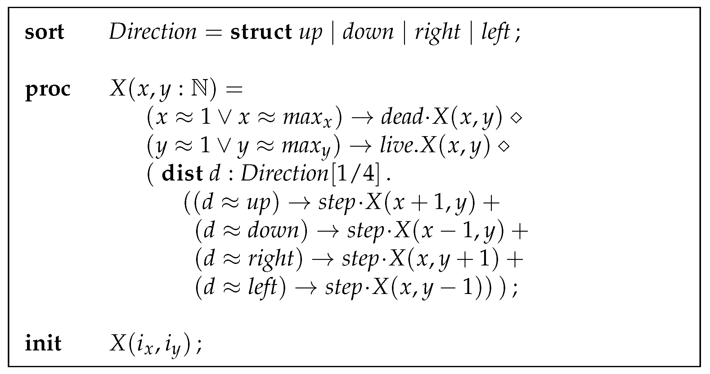
The specification in probabilistic mCRL2 of the ant-on-a-grid is given in Figure 4, where the dimensions of the grid are ${\mathit{max}}_x$ and ${\mathit{max}}_y$, and the initial position is given by $i_x$ and $i_y$.

The actions $\mathit{dead}$, $\mathit{live}$ and $\mathit{step}$ indicate that the ant is dead, stays alive and makes a step. The process expression $p·q$ stands for sequential composition and $p+q$ represents the choice in behaviour. The notations $c\to p$ and $c\to p\diamond q$ are the if-then and if-then-else of mCRL2. The curly equal sign (≈) in conditions stands for equality applied to data expressions. The expression $\mathbf{dist}d:\mathit{Direction}[1/4]$ means that each direction d is chosen with probability $\frac{1}{4}$. From this description, PLTSs are generated that are used as input for the probabilistic bisimulation reduction tools.

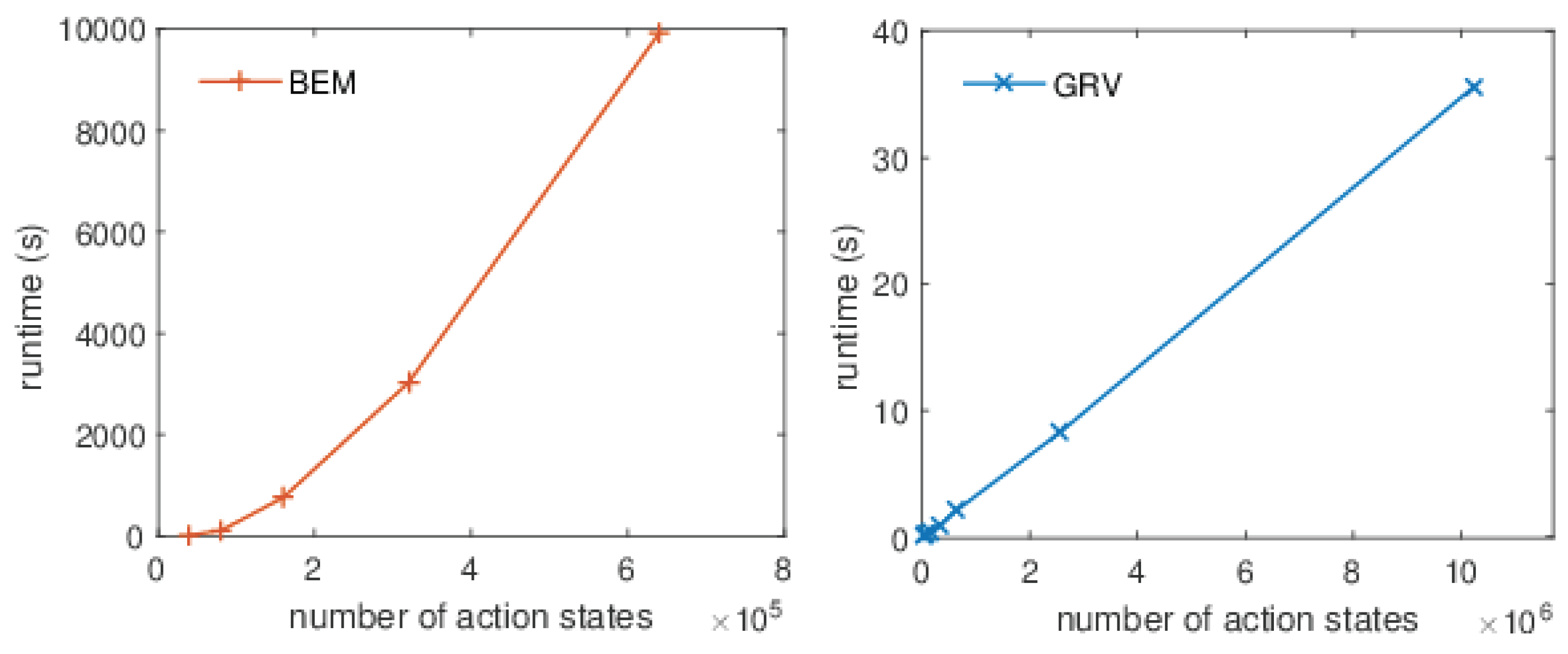
Figure 5 depicts the runtime results of a set of experiments when increasing the total number of states of the ant on the grid model. At the left are the results when running the BEM algorithm, whereas the results for the GRV algorithm are shown at the right. Note that the x-axis only depicts the number of action states. This figure indicates that the practical running times of both algorithms are pretty much in line with the theoretical complexity. This is in agreement with our findings on other examples as well. Furthermore, it should be noted that the difference in performance is dramatic. The largest example that our implementation of the BEM algorithm can handle within a timeout of 5 h requires approximately 10,000 s compared to 2 s for GRV. The particular example regards a PLTS of $6.4\times {10}^5$ action states. The graphs clearly indicate that the difference grows when the probabilistic transition systems get larger.

To further understand the practical usability of the GRV algorithm, we applied it to a number of benchmarks taken from the PRISM Benchmark Suite (www.prismmodelchecker.org/benchmarks/) and the mCRL2 toolset (www.mcrl2.org/). The tests taken from PRISM were first translated into mCRL2 code to generate the corresponding PLTSs.

Table 3. Runtime (in s) and memory use (in MB) results for the reference algorithm (BEM) and the GRV algorithm.

Model	${\mathit{n}}_{\mathit{a}}$	${\mathit{m}}_{\mathit{a}}$	${\mathit{n}}_{\mathit{p}}$	${\mathit{m}}_{\mathit{p}}$	min. ${\mathit{n}}_{\mathit{a}}$	min. ${\mathit{m}}_{\mathit{a}}$	min. ${\mathit{n}}_{\mathit{p}}$	min. ${\mathit{m}}_{\mathit{p}}$	timeBEM	me.BEM	timeGRV	me.GRV	Speed-up	Memory
shared_coin_2_5	14,096	28,192	12,891	14,801	998	1995	1163	1479	5.45	53.57	0.08	51.34	68	1.04
brp_100_20	15,003	15,003	10,803	15,003	8504	8504	8504	12,704	37.27	82.51	0.06	55.79	621	1.48
self_stab_7	16,130	56,462	14,337	57,346	2060	9324	2836	5672	14.08	71.54	0.17	66.35	83	1.08
brp_100_40	29,003	29,003	20,803	29,003	16,504	16,504	16,504	24,704	368.67	176.34	0.22	65.41	1676	2.70
airplane_4000	31,991	31,990	15,998	31,991	23,995	23,994	15,998	23,995	491.75	219.01	0.15	66.88	3278	3.27
ant_100_100_grid	39,984	39,984	9997	39,988	2405	2405	2404	9608	18.52	78.08	0.14	61.85	132	1.26
random_40	40,000	63,981	54,123	86,231	29,610	60,864	45,092	73,861	1766.80	546.21	0.50	111.70	3534	4.89
shared_coin_2_10	53,736	107K	48,131	551K	1978	3955	2303	2939	65.41	107.85	0.36	81.34	182	1.33
self_stab_8	65,026	260K	65,537	262K	6306	32,960	9721	19,442	401.17	294.44	0.69	157.17	581	1.87
brp_200_50	72,003	72,003	51,603	72,003	41,004	41,004	41,004	61,404	1674.53	814.89	0.38	101.86	4407	8.00
ant_200_100_grid	79,984	79,984	19,997	79,988	4855	4855	4854	19,408	105.78	164.55	0.20	82.85	529	1.99
airplane_10000	79,991	79,990	39,998	79,991	59,995	59,994	39,998	59,995	2805.12	1073.63	0.37	113.83	7581	9.43
random_100	100K	160K	134K	215K	73,607	151K	112K	183K	15,439.18	2975.38	1.14	213.08	13,534	13.96
ant_200_200_grid	160K	160K	39,997	160K	9805	9805	9804	39,208	760.17	484.78	0.41	124.84	1854	3.88
shared_coin_2_20	210K	419K	185K	212K	3938	7875	4583	5859	654.94	440.18	1.19	198.80	550	2.21
self_stab_9	262K	1175K	294K	1180K	19,172	113K	32,806	65,612	4015.53	2809.32	3.24	598.14	1239	4.70
shared_coin_3_2	280K	837K	274K	318K	5841	17,347	7722	10,068	1781.64	974.92	1.78	294.68	1001	3.31
ant_400_200_grid	320K	320K	79,997	320K	19,705	19,705	19,704	78,808	3026.02	1703.80	0.88	218.95	3439	7.78
airplane_40000	320K	320K	160K	320K	240K	240K	160K	240K	-	-	1.34	333.17	-	-
random_400	400K	638K	540K	859K	293K	605K	446K	730K	-	-	5.11	729.84	-	-
shared_coin_2_30	468K	936K	413K	472K	5898	11,795	6863	8779	2427.55	1248.44	2.95	389.13	823	3.21
ant_400_400_grid	640K	640K	160K	640K	39,605	39,605	39,604	158K	9917.64	6477.75	2.09	397.23	4745	16.31
airplane_100000	800K	800K	400K	800K	600K	600K	400K	600K	-	-	4.22	755.948	-	-
random_800	800K	1277K	1079K	1718K	587K	1210K	893K	1462K	-	-	11.98	1418.79	-	-
brp_600_200	846K	846K	604K	846K	483K	483K	483K	724K	-	-	4.94	789.05	-	-
self_stab_10	1046K	5232K	1311K	5242K	58,026	383K	109K	218K	-	-	16.53	2369.75	-	-
shared_coin_2_60	1858K	3716K	1632K	1866K	11,778	23,555	13,703	17,539	-	-	12.25	1416.92	-	-
ant_800_800_grid	2560K	2560K	640K	2560K	159K	159K	159K	636K	-	-	8.27	1466.44	-	-
shared_coin_3_5	3222K	9665K	2984K	3437K	14,085	41,863	18,630	24,432	-	-	26.97	2809.88	-	-
brp_1000_500	3510K	3510K	2508K	3510K	2005K	2005K	2005K	3007K	-	-	24.85	3122.14	-	-
ant_1600_1600_grid	10,240K	10,240K	2560K	10,240K	638K	638K	638K	2553K	-	-	35.64	5743.74	-	-
brp_2000_1000	14,020K	14,020K	10,016K	14,020K	8010K	8010K	8010K	12,015K	-	-	115.95	12,351.47	-	-
brp_4000_2000	56,040K	56,040K	40,032K	56,040K	32,020K	32,020K	32,020K	48,030K	-	-	652.78	49,253.50	-	-

collects the results for the experiments conducted. The ant_N_M_grid examples refer to the ant-on-a-grid puzzle for an N by M grid with the ant initially placed at the approximate center of the grid. The models airplane_N are instances of an airplane ticket problem using N seats. In the airplane ticket problem, N passengers enter a plane. The first passenger lost his boarding pass and therefore takes a random seat. Each subsequent passenger will take his own seat unless it is already taken, in which case he randomly selects an empty seat as well. The intriguing question is to determine the probability that the last passenger will have his or her own seat (see [28] for a more detailed account).

The following three benchmarks stem from PRISM: The brp_N_MAX models are instances of the bounded retransmission protocol when transmitting N packages and bounding the number of retransmissions to $\mathit{MAX}$. The self_stab_N and shared_coin_N_K are extensions of the self stabilisation protocol and the shared coin protocol, respectively. For the self stabilisation protocol, N processes are involved in the protocol, each holding a token initially. The shared coin protocol is modelled using N processes and setting the threshold to decide head or tail to K.

Finally, the random_N tests are randomly generated PLTSs with N action states. All the models are available in the mCRL2 toolset.

At the left of Table 3, the characteristics for each PLTS are given: the number of action states ($n_a$), the number of action transitions ($m_a$), the number of distributions ($n_p$), and the cumulative support of the distributions ($m_p$). The symbol “K” is an indicator for 1000 states. The same characteristics for the minimised PLTS are also provided. Furthermore, the runtime for minimising the probabilistic transition system in seconds as well as the required memory in megabytes are indicated for both algorithms. As mentioned earlier, we limited the runtime to 5 h.

The experiments show that the GRV algorithm outperforms the reference algorithm quite substantially in all studied cases. In the case of “random_100” the difference is four orders of magnitude, despite the fact that this state space has only 100 K action states. The second last column of Table 3 lists the relative speed-up, i.e. the quotient of the time needed by BEM over the time needed by GRV, when applicable. Memory usage is comparable for both algorithms for small cases, whereas for larger examples the BEM algorithm requires up to one order of magnitude more memory than the GRV algorithm. The right-most column of Table 3 contains the relative efficiency in memory, i.e. the quotient of the memory used by BEM over the memory used by GRV, for the cases where BEM terminated before the deadline.

6. Concluding Remarks

We believe we have formulated a very efficient algorithm to determine probabilistic bisimulation. As the algorithm restricts the handling of distributions to the states in the support of the distributions, the running time of the algorithm compares favourably when the fan-out is low in the PLTS under consideration, a situation occurring frequently in practice.

Apart from deciding strong probabilistic bisimilarity, our algorithm is instrumental in the mCRL2 toolset for minimising PLTSs modulo probabilistic bisimulation. Such a reduction can be useful as a preprocessing step before applying other forms of analysis on the PLTS. Occasionally, minimisation can even simplify PLTSs such that they become suitable for visual inspection. See for example the discussion the airplane ticket problem, also known as the problem of the lost boarding pass, in [28]. However, having smaller state spaces will be beneficial regardless, as this reduces the processing time for other tools further down the analysis chain.

To fine tune the algorithm, it will be interesting in future work to investigate how to choose the non-trivial constellations C and its sub-blocks $B_C$ optimally; their choice is now non-deterministic. Furthermore, it is interesting to refine the algorithm to probabilistic bisimulation with combined transitions [29] as this appears to be required to extend this algorithm to weaker notions of equivalence [21], such as probabilistic branching bisimulation.

References