Degradation Trend Prediction for Rotating Machinery Using Long-Range Dependence and Particle Filter Approach


Abstract
1. Introduction
- (1)
- If the fractional order or LRD property of the health indicator time series (HITS) is too weak (e.g., the Hurst exponent approaching 0.5), especially the time series at the stationary operation stage, the f-ARIMA and FBM models might become unusable and the prediction accuracy reduced dramatically if the classical FOC model lacks the optimal solution.
- (2)
- Similar to the physics-based model, the model parameters of the classical LRD model such as f-ARIMA cannot be adjusted with the evolution of an actual degeneration trend of the HITS, and the prediction accuracies are also greatly decreased.
- (3)
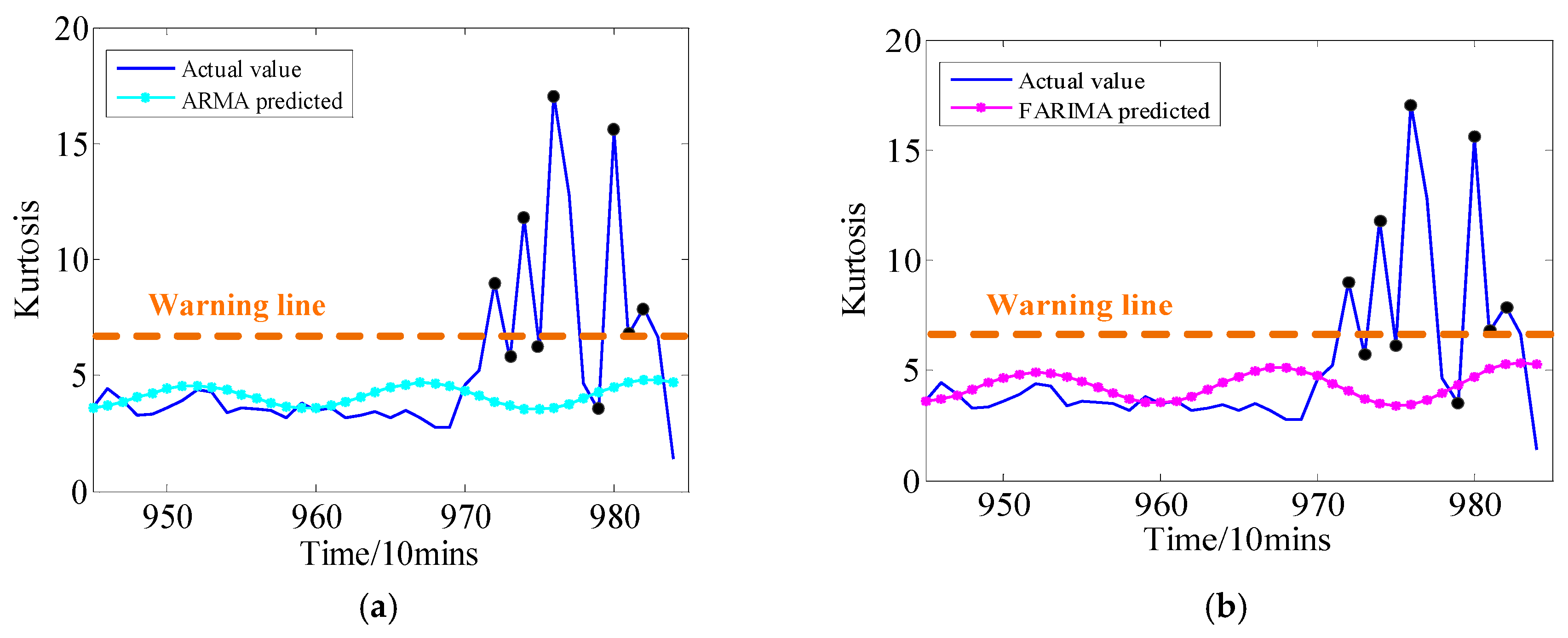
- If some sharp transition points (STPs) are contained in the health indicator time series (HITS), especially the time series at the incipient/severe fault phase, the traditional f-ARIMA and FOC approaches treat all time series values equally, which ignore the fact that the STPs value should be preserved at a larger weight, thus limiting their effectiveness in practical application.
2. Fractional Gaussian Noise and LRD Model
3. Particle Filter Frame
3.1. Bayesian Filter Algorithm
- (1)
- Suppose the prior probability distribution is known, the number of samples is N from the posterior distribution according to Equation (7). Considering the first-order Markov process, the approximation of the posterior distribution can be given by,
- (2)
- The posterior distribution function estimation can be updated by the Bayes formula as follows,where is likelihood function at time k, and is the normalizing constant which can be calculated as follow,
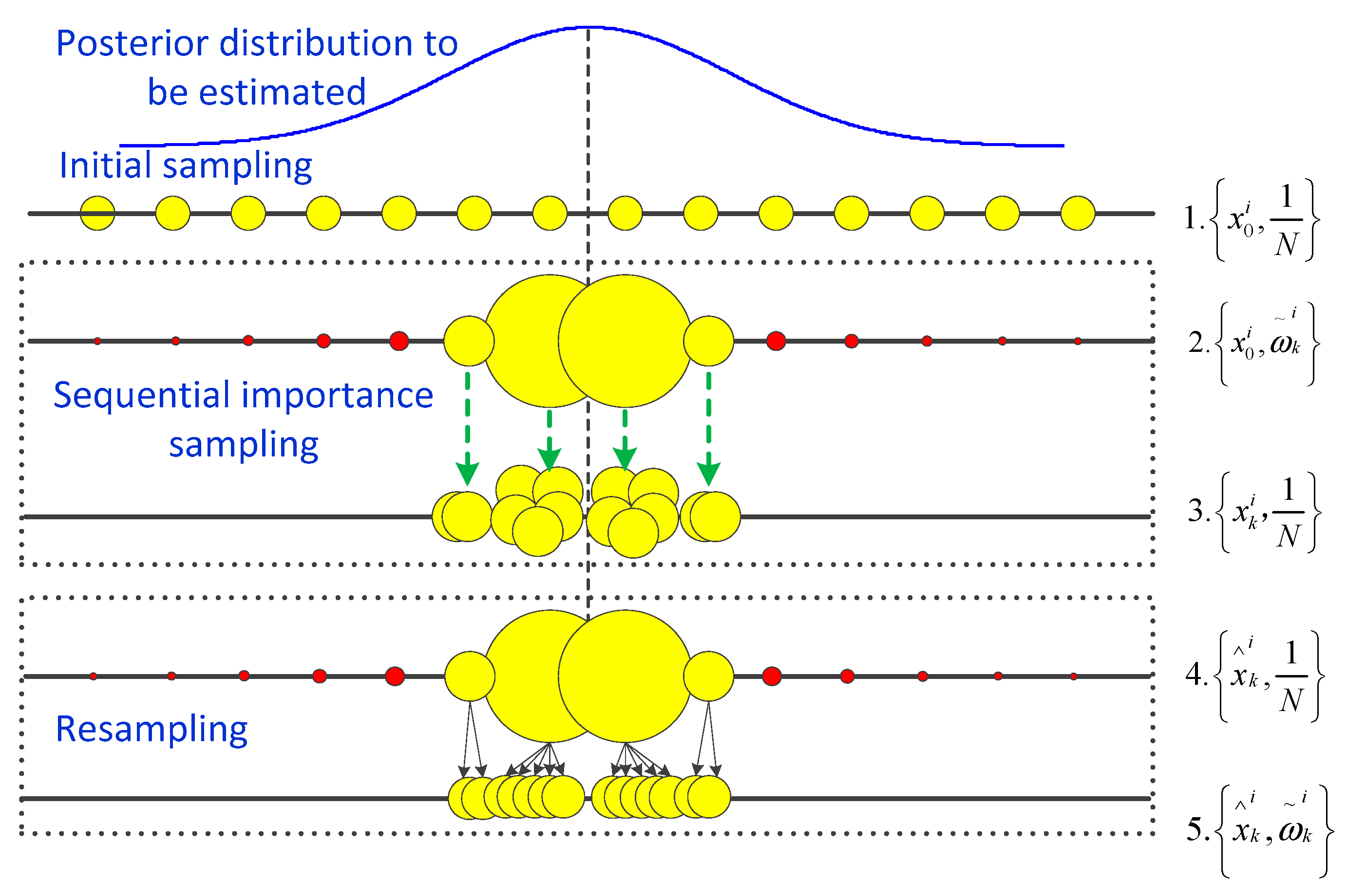
3.2. Particle Filter Frame Algorithm
- (a)
- Initialization.Sampling N particles from the prior probability distribution function, and the initialization weight is accordingly.
- (b)
- Sequential importance sampling (SIS).
- (1)
- Resample independently N times from the above discrete distribution.
- (2)
- The prior weights are used to update the new weights, as follow,where is the likelihood function.
- (3)
- Normalize the importance weights, i.e., , where is the normalized weight of the i-th particle at time k, and N the number of particles.
- (c)
- Resampling.
3.3. LRD Predicting Operator Driven by Particle Filter Frame
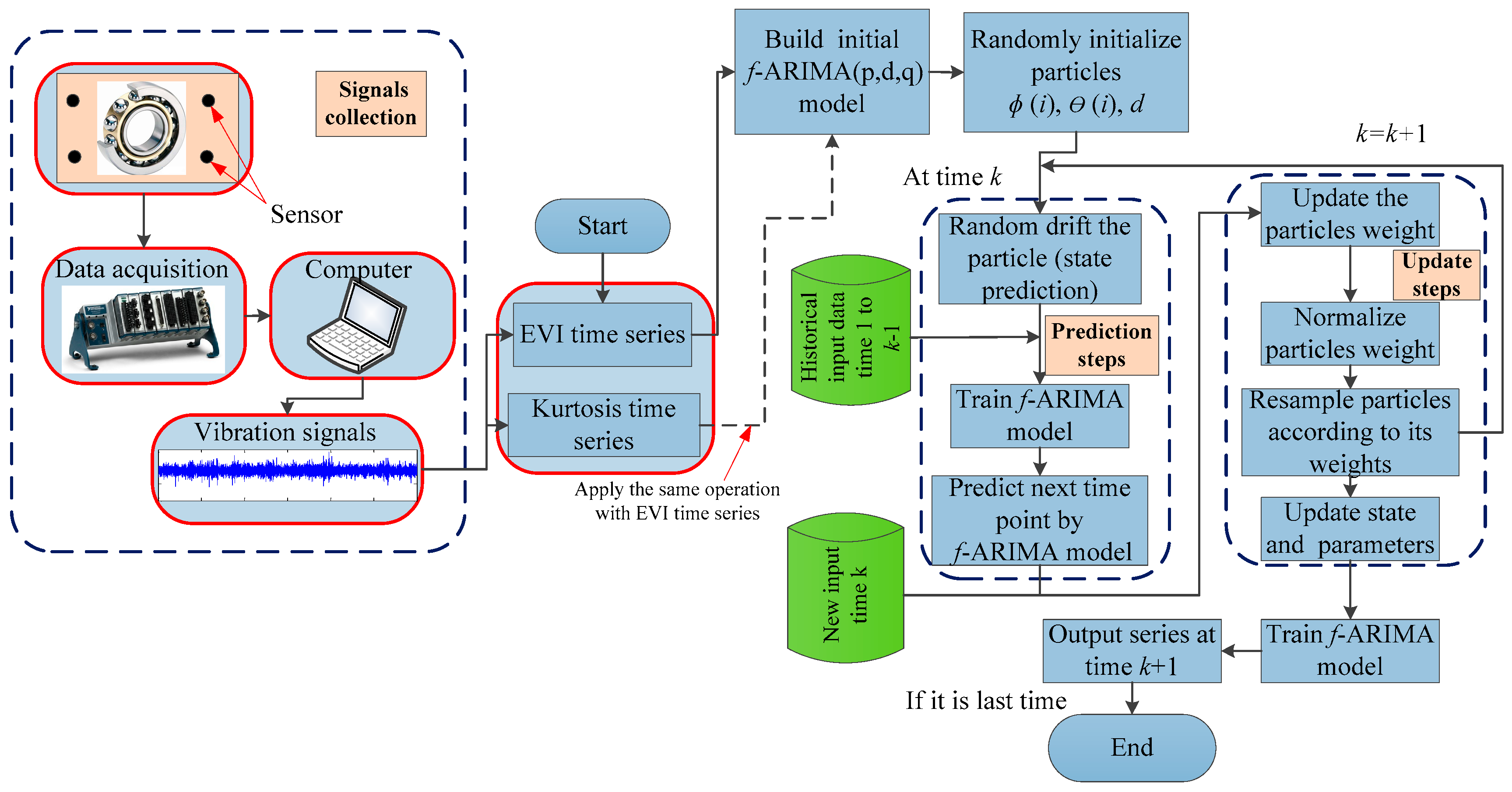
- Step 1.
- Particle initialization.
- (a)
- The f-ARIMA degradation models are established by the tested EVI time series or kurtosis time series. In this stage, the initial f-ARIMA model order and coefficients distribution are determined, i.e., , where p and q are model orders, d0 is initial fractional value, and ϕ(i) and θ(i) are model coefficients.
- (b)
- By drifting all of the coefficients set randomly, that is, , where is noise sequence, then the particles set is obtained, the number of particles set is N, and their weights are initialized as .
- Step 2.
- For k = 1, 2, …, L (L is step length):
- (a)
- For k = k − 1, predict the time series output one-step by f-ARIMA model with the parameters .
- (b)
- When the new output time series point yk arrives, update each particle’s weight: .
- (c)
- Normalize the particles weight, i.e., .
- (d)
- Resampling is performed to remove the small weight particles and generate promising new particles with the larger weight, thus the new particles set is .
- Step 3.
- The state vector can be estimated as .
- Step 4.
- Train the f-ARIMA model using the update state vector to get the prediction value of .
- Step 5.
- Algorithm stops when k is equal to step length L, otherwise, go to step (2).
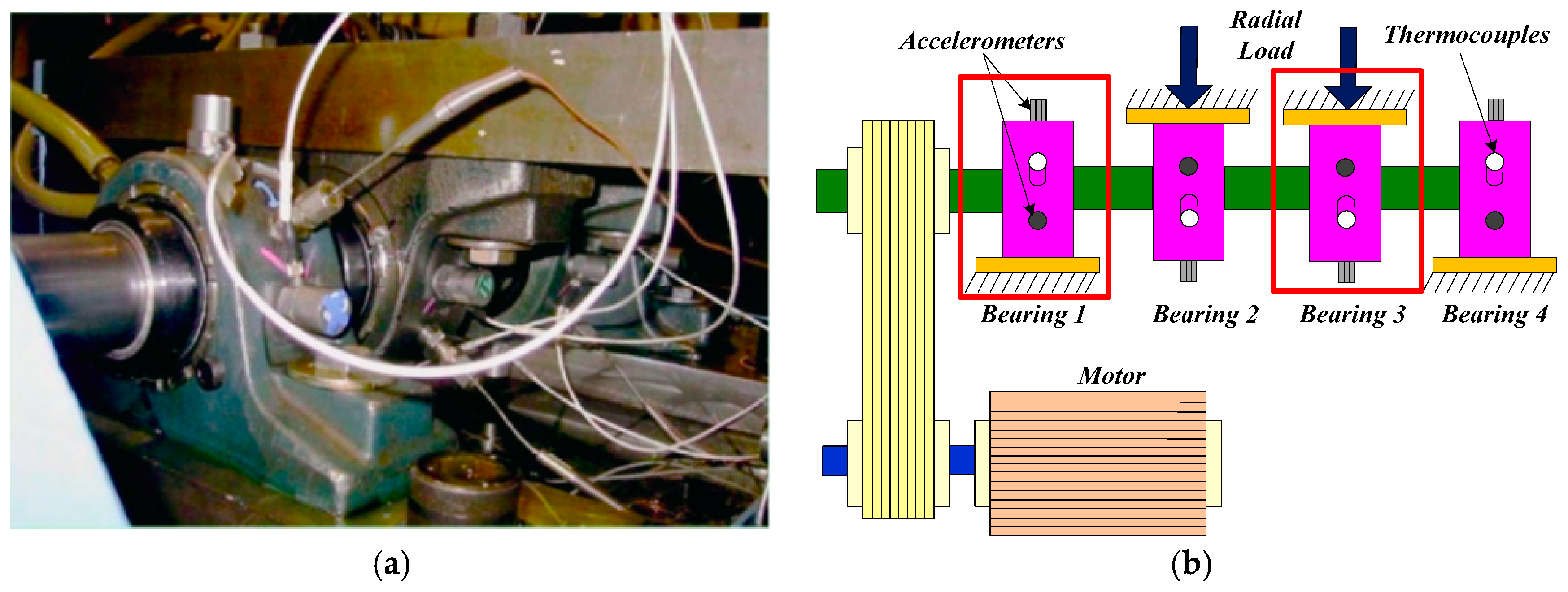
4. Experimental Evaluations
4.1. Experimental Setup
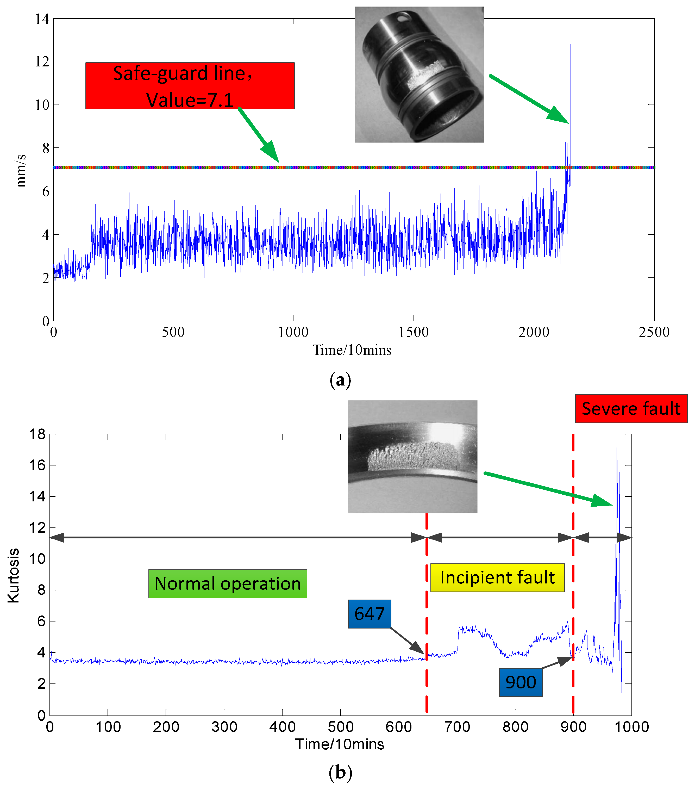
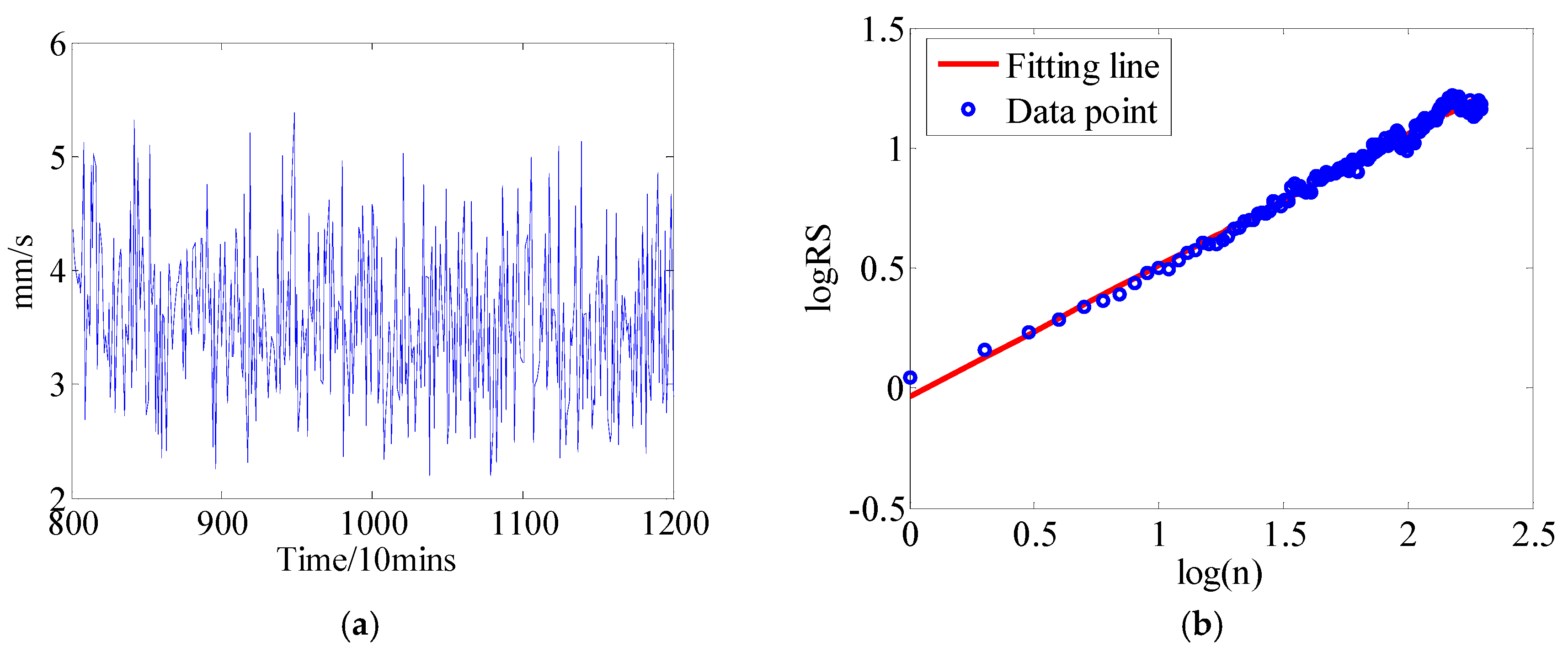
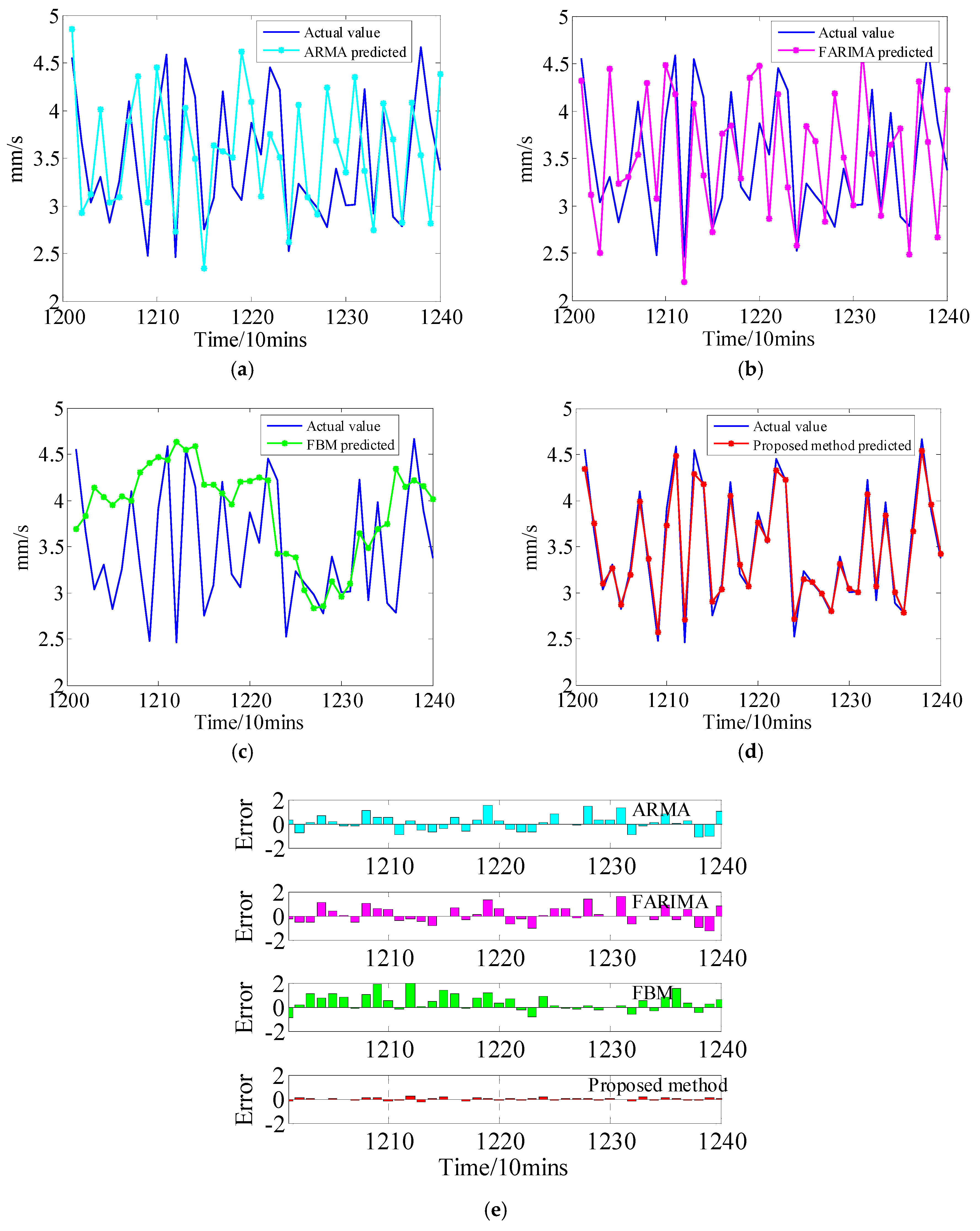
4.2. Case 1: The EVI Time Series with Weak LRD Property
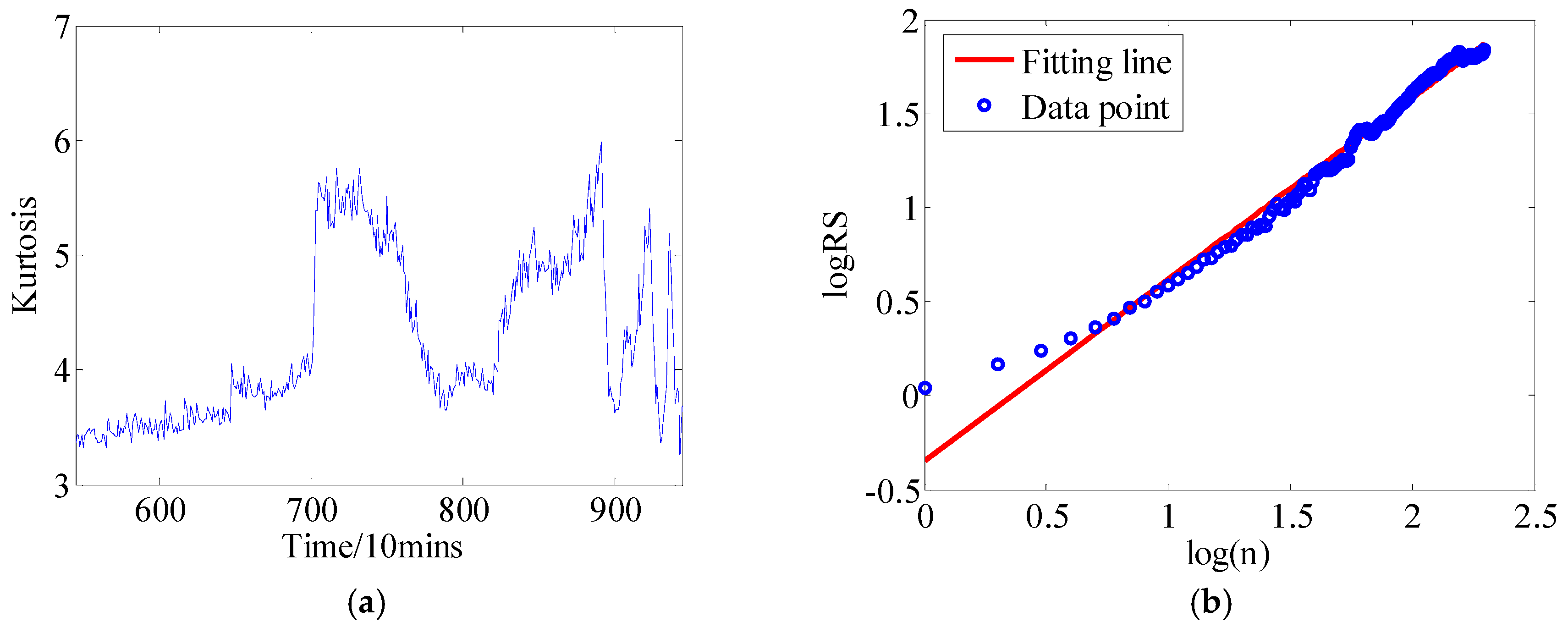
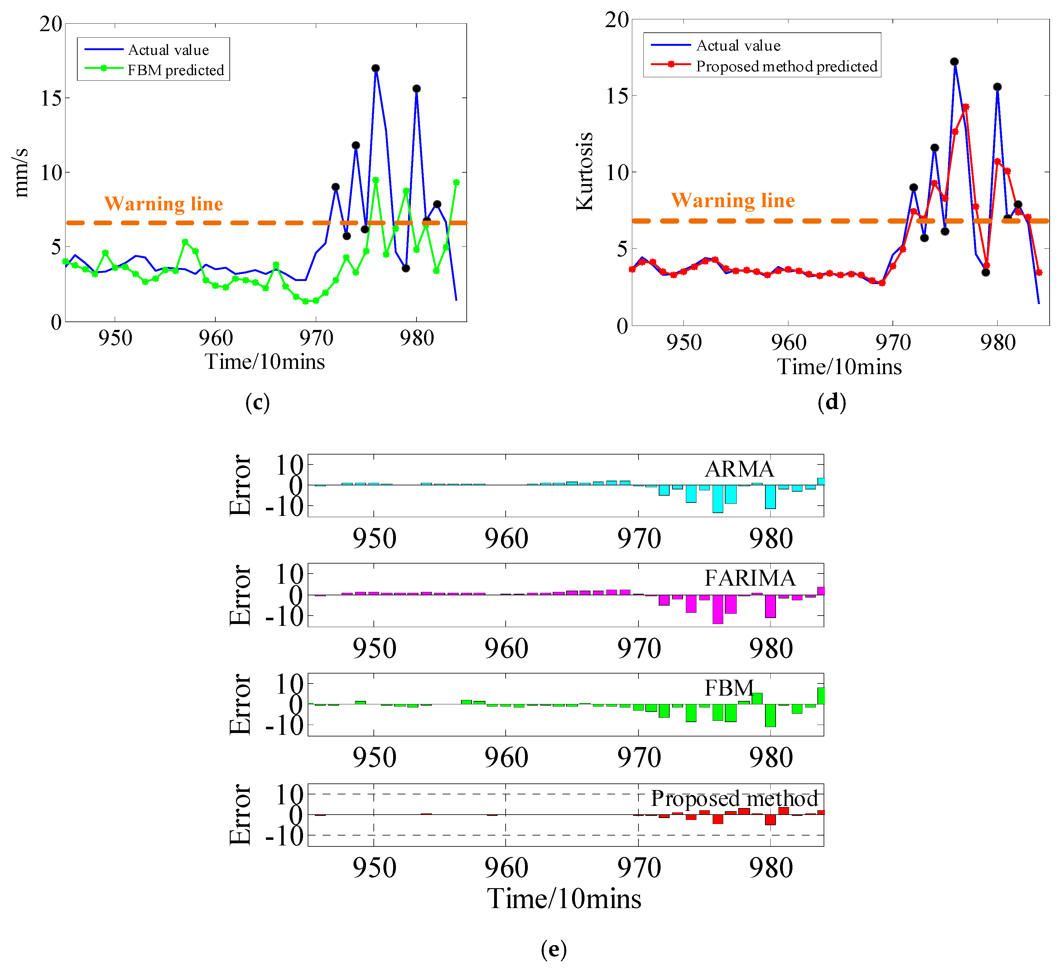
4.3. Case 2: The Kurtosis Time Series with STPs
5. Conclusions
- (1)
- For engineering applications, a new condition prognostic method is introduced as an effective tool for the long lifetime prediction and assessment of mechanical equipment in the PHM filed, the mechanical running degradation pattern can be predicted well in real-time and the most vital components of the mechanical equipment can be repaired and replaced prior to actual catastrophic failure.
- (2)
- For theoretical analysis, the particle filter frame (PFF) is embedded in the FOC model, an update scheme for online model parameters has been introduced to adapt the initial state model based on the PFF algorithm. Due to the adaptability of the parameters, the performance of our proposed model is remarkably efficient than classical time-series ARMA model and the FOC models, even the initial health status is unknown and the failure degradation behavior is time-varying. That is to say, the main advantage of the proposed approach is that the prognostic model has an ability to generate the reliable probabilistic results despite the uncertainties of the initial model parameters.
Author Contributions
Acknowledgments
Conflicts of Interest
Appendix A

| Real | ARMA | Error | RE | FARIMA | Error | RE | FBM | Error | RE | Proposed | Error | RE |
|---|---|---|---|---|---|---|---|---|---|---|---|---|
| 4.5522 | 4.851179 | 0.298979 | 0.065678 | 4.315315 | −0.23689 | 0.052038 | 3.692463 | −0.85974 | 0.188862 | 4.338669 | −0.21353 | 0.046907 |
| 3.6649 | 2.928812 | −0.73609 | 0.200848 | 3.116309 | −0.54859 | 0.149688 | 3.829959 | 0.165059 | 0.045038 | 3.754522 | 0.089622 | 0.024454 |
| 3.036 | 3.122478 | 0.086478 | 0.028484 | 2.500855 | −0.53514 | 0.176266 | 4.138178 | 1.102178 | 0.363036 | 3.1013 | 0.0653 | 0.021508 |
| 3.3038 | 4.012963 | 0.709163 | 0.214651 | 4.443229 | 1.139429 | 0.344884 | 4.036887 | 0.733087 | 0.221892 | 3.262692 | −0.04111 | 0.012443 |
| 2.8203 | 3.032396 | 0.212096 | 0.075203 | 3.228642 | 0.408342 | 0.144787 | 3.947579 | 1.127279 | 0.399702 | 2.87064 | 0.05034 | 0.017849 |
| 3.2525 | 3.090151 | −0.16235 | 0.049915 | 3.305279 | 0.052779 | 0.016227 | 4.043051 | 0.790551 | 0.243059 | 3.19275 | −0.05975 | 0.018371 |
| 4.1008 | 3.887408 | −0.21339 | 0.052037 | 3.536877 | −0.56392 | 0.137515 | 3.998855 | −0.10194 | 0.02486 | 3.985144 | −0.11566 | 0.028203 |
| 3.2772 | 4.359959 | 1.082759 | 0.330391 | 4.294689 | 1.017489 | 0.310475 | 4.301419 | 1.024219 | 0.312529 | 3.362803 | 0.085603 | 0.026121 |
| 2.4798 | 3.038506 | 0.558706 | 0.225303 | 3.073638 | 0.593838 | 0.23947 | 4.407019 | 1.927219 | 0.777167 | 2.569523 | 0.089723 | 0.036181 |
| 3.9129 | 4.451459 | 0.538559 | 0.137637 | 4.483454 | 0.570554 | 0.145814 | 4.465283 | 0.552383 | 0.14117 | 3.731065 | −0.18184 | 0.046471 |
| 4.5876 | 3.712715 | −0.87489 | 0.190707 | 4.176524 | −0.41108 | 0.089606 | 4.436422 | −0.15118 | 0.032954 | 4.487611 | −0.09999 | 0.021795 |
| 2.4631 | 2.732075 | 0.268975 | 0.109202 | 2.190463 | −0.27264 | 0.110689 | 4.635023 | 2.171923 | 0.881784 | 2.706797 | 0.243697 | 0.098939 |
| 4.55 | 4.025714 | −0.52429 | 0.115228 | 4.073607 | −0.47639 | 0.104702 | 4.550027 | 2.66×10⁻⁵ | 5.84×10⁻⁶ | 4.286559 | −0.26344 | 0.057899 |
| 4.146 | 3.494402 | −0.6516 | 0.157163 | 3.316627 | −0.82937 | 0.200042 | 4.588838 | 0.442838 | 0.106811 | 4.175007 | 0.029007 | 0.006996 |
| 2.7487 | 2.343199 | −0.4055 | 0.147525 | 2.717725 | −0.03097 | 0.011269 | 4.165975 | 1.417275 | 0.515617 | 2.905444 | 0.156744 | 0.057025 |
| 3.0865 | 3.63355 | 0.54705 | 0.17724 | 3.757182 | 0.670682 | 0.217295 | 4.169485 | 1.082985 | 0.350878 | 3.03899 | −0.04751 | 0.015393 |
| 4.1998 | 3.571195 | −0.62861 | 0.149675 | 3.843438 | −0.35636 | 0.084852 | 4.076447 | −0.12335 | 0.029371 | 4.052326 | −0.14747 | 0.035115 |
| 3.1988 | 3.510075 | 0.311275 | 0.09731 | 3.290616 | 0.091816 | 0.028703 | 3.958997 | 0.760197 | 0.237651 | 3.30548 | 0.10668 | 0.03335 |
| 3.0569 | 4.620933 | 1.564033 | 0.51164 | 4.349495 | 1.292595 | 0.422845 | 4.201031 | 1.144131 | 0.374278 | 3.065222 | 0.008322 | 0.002722 |
| 3.8719 | 4.094481 | 0.222581 | 0.057486 | 4.475258 | 0.603358 | 0.15583 | 4.209925 | 0.338025 | 0.087302 | 3.761908 | −0.10999 | 0.028408 |
| 3.5429 | 3.102141 | −0.44076 | 0.124406 | 2.865971 | −0.67693 | 0.191066 | 4.244785 | 0.701885 | 0.19811 | 3.568503 | 0.025603 | 0.007227 |
| 4.4554 | 3.754243 | −0.70116 | 0.157372 | 4.179654 | −0.27575 | 0.06189 | 4.216189 | −0.23921 | 0.05369 | 4.328812 | −0.12659 | 0.028412 |
| 4.2155 | 3.506033 | −0.70947 | 0.1683 | 3.196617 | −1.01888 | 0.241699 | 3.419768 | −0.79573 | 0.188763 | 4.224678 | 0.009178 | 0.002177 |
| 2.521 | 2.621368 | 0.100368 | 0.039813 | 2.579941 | 0.058941 | 0.02338 | 3.423397 | 0.902397 | 0.357952 | 2.714081 | 0.193081 | 0.076589 |
| 3.2362 | 4.057441 | 0.821241 | 0.253767 | 3.836757 | 0.600557 | 0.185575 | 3.377986 | 0.141786 | 0.043813 | 3.143407 | −0.09279 | 0.028673 |
| 3.1059 | 3.091177 | −0.01472 | 0.00474 | 3.682622 | 0.576722 | 0.185686 | 3.026959 | −0.07894 | 0.025416 | 3.112301 | 0.006401 | 0.002061 |
| 2.9839 | 2.908971 | −0.07493 | 0.025111 | 2.831969 | −0.15193 | 0.050917 | 2.832535 | −0.15137 | 0.050727 | 2.990418 | 0.006518 | 0.002184 |
| 2.7785 | 4.240453 | 1.461953 | 0.526166 | 4.188664 | 1.410164 | 0.507527 | 2.850715 | 0.072215 | 0.025991 | 2.796518 | 0.018018 | 0.006485 |
| 3.3918 | 3.682935 | 0.291135 | 0.085835 | 3.509299 | 0.117499 | 0.034642 | 3.124385 | −0.26741 | 0.078842 | 3.309347 | −0.08245 | 0.02431 |
| 3.0046 | 3.348826 | 0.344226 | 0.114566 | 3.001548 | −0.00305 | 0.001016 | 2.957211 | −0.04739 | 0.015772 | 3.041626 | 0.037026 | 0.012323 |
| 3.0101 | 4.347179 | 1.337079 | 0.444197 | 4.64161 | 1.63151 | 0.542012 | 3.099322 | 0.089222 | 0.029641 | 3.001522 | −0.00858 | 0.00285 |
| 4.226 | 3.36362 | −0.86238 | 0.204065 | 3.548991 | −0.67701 | 0.160201 | 3.639928 | −0.58607 | 0.138682 | 4.066107 | −0.15989 | 0.037836 |
| 2.9203 | 2.747795 | −0.1725 | 0.059071 | 2.890067 | −0.03023 | 0.010353 | 3.486781 | 0.566481 | 0.19398 | 3.064534 | 0.144234 | 0.04939 |
| 3.9785 | 4.071772 | 0.093272 | 0.023444 | 3.644438 | −0.33406 | 0.083967 | 3.687806 | −0.29069 | 0.073066 | 3.839084 | −0.13942 | 0.035042 |
| 2.8849 | 3.696822 | 0.811922 | 0.281438 | 3.812164 | 0.927264 | 0.32142 | 3.740511 | 0.855611 | 0.296583 | 3.004821 | 0.119921 | 0.041569 |
| 2.781 | 2.821017 | 0.040017 | 0.014389 | 2.481329 | −0.29967 | 0.107757 | 4.339559 | 1.558559 | 0.560431 | 2.787078 | 0.006078 | 0.002185 |
| 3.8017 | 4.081894 | 0.280194 | 0.073702 | 4.310372 | 0.508672 | 0.133801 | 4.144882 | 0.343182 | 0.090271 | 3.668168 | −0.13353 | 0.035124 |
| 4.6639 | 3.529533 | −1.13437 | 0.243223 | 3.672363 | −0.99154 | 0.212598 | 4.21923 | −0.44467 | 0.095343 | 4.540967 | −0.12293 | 0.026358 |
| 3.8834 | 2.812674 | −1.07073 | 0.275719 | 2.667587 | −1.21581 | 0.313079 | 4.152104 | 0.268704 | 0.069193 | 3.957954 | 0.074554 | 0.019198 |
| 3.3754 | 4.384567 | 1.009167 | 0.298977 | 4.223374 | 0.847974 | 0.251222 | 4.010072 | 0.634672 | 0.188029 | 3.422911 | 0.047511 | 0.014076 |
| Real | ARMA | Error | RE | FARIMA | Error | RE | FBM | Error | RE | Proposed | Error | RE |
|---|---|---|---|---|---|---|---|---|---|---|---|---|
| 3.643158 | 3.583676 | −0.05948 | 0.016327 | 3.573756 | −0.0694 | 0.01905 | 4.032532 | 0.389374 | 0.106878 | 3.658809 | 0.015651 | 0.004296 |
| 4.458712 | 3.72162 | −0.73709 | 0.165315 | 3.698368 | −0.76034 | 0.17053 | 3.767629 | −0.69108 | 0.154996 | 4.125354 | −0.33336 | 0.074765 |
| 3.885578 | 3.867426 | −0.01815 | 0.004672 | 3.848826 | −0.03675 | 0.009459 | 3.486229 | −0.39935 | 0.102777 | 4.097066 | 0.211488 | 0.054429 |
| 3.26448 | 4.058685 | 0.794206 | 0.243287 | 4.109618 | 0.845139 | 0.258889 | 3.156036 | −0.10844 | 0.033219 | 3.507751 | 0.243271 | 0.074521 |
| 3.326908 | 4.248171 | 0.921263 | 0.276913 | 4.428144 | 1.101236 | 0.331009 | 4.602094 | 1.275186 | 0.383295 | 3.306727 | −0.02018 | 0.006066 |
| 3.596278 | 4.40949 | 0.813212 | 0.226126 | 4.669793 | 1.073515 | 0.298507 | 3.575741 | −0.02054 | 0.005711 | 3.490924 | −0.10535 | 0.029295 |
| 3.911841 | 4.51446 | 0.602619 | 0.15405 | 4.809623 | 0.897783 | 0.229504 | 3.624969 | −0.28687 | 0.073334 | 3.781957 | −0.12988 | 0.033203 |
| 4.374046 | 4.545397 | 0.171351 | 0.039175 | 4.892967 | 0.518921 | 0.118636 | 3.181498 | −1.19255 | 0.272642 | 4.17795 | −0.1961 | 0.044832 |
| 4.252138 | 4.496206 | 0.244068 | 0.057399 | 4.834369 | 0.582232 | 0.136927 | 2.674354 | −1.57778 | 0.371057 | 4.28264 | 0.030502 | 0.007173 |
| 3.393007 | 4.374221 | 0.981215 | 0.289187 | 4.699951 | 1.306944 | 0.385188 | 2.841052 | −0.55195 | 0.162674 | 3.724723 | 0.331716 | 0.097765 |
| 3.612475 | 4.199098 | 0.586623 | 0.162388 | 4.481938 | 0.869463 | 0.240683 | 3.447842 | −0.16463 | 0.045574 | 3.52586 | −0.08662 | 0.023977 |
| 3.561138 | 3.999812 | 0.438674 | 0.123184 | 4.222849 | 0.661711 | 0.185815 | 3.387714 | −0.17342 | 0.048699 | 3.579461 | 0.018323 | 0.005145 |
| 3.465567 | 3.809977 | 0.34441 | 0.099381 | 3.963394 | 0.497827 | 0.14365 | 5.315971 | 1.850404 | 0.53394 | 3.502904 | 0.037337 | 0.010774 |
| 3.168745 | 3.662308 | 0.493563 | 0.15576 | 3.700369 | 0.531624 | 0.167771 | 4.683602 | 1.514857 | 0.478062 | 3.289646 | 0.120902 | 0.038154 |
| 3.819911 | 3.583102 | −0.23681 | 0.061993 | 3.562851 | −0.25706 | 0.067295 | 2.746134 | −1.07378 | 0.2811 | 3.56325 | −0.25666 | 0.06719 |
| 3.500932 | 3.587702 | 0.08677 | 0.024785 | 3.53361 | 0.032678 | 0.009334 | 2.37261 | −1.12832 | 0.322292 | 3.623144 | 0.122212 | 0.034908 |
| 3.570946 | 3.677685 | 0.106739 | 0.029891 | 3.616021 | 0.045075 | 0.012623 | 2.29524 | −1.27571 | 0.357246 | 3.54248 | −0.02847 | 0.007972 |
| 3.168281 | 3.840316 | 0.672035 | 0.212113 | 3.826746 | 0.658465 | 0.20783 | 2.838346 | −0.32994 | 0.104137 | 3.329741 | 0.16146 | 0.050961 |
| 3.293096 | 4.05039 | 0.757294 | 0.229964 | 4.099097 | 0.806001 | 0.244755 | 2.776671 | −0.51643 | 0.156821 | 3.249593 | −0.0435 | 0.01321 |
| 3.446315 | 4.274201 | 0.827886 | 0.240224 | 4.429192 | 0.982877 | 0.285197 | 2.604462 | −0.84185 | 0.244276 | 3.388605 | −0.05771 | 0.016745 |
| 3.162353 | 4.475022 | 1.312669 | 0.415092 | 4.722749 | 1.560396 | 0.493429 | 2.233966 | −0.92839 | 0.293575 | 3.278397 | 0.116044 | 0.036696 |
| 3.466872 | 4.619211 | 1.152339 | 0.332386 | 4.955867 | 1.488995 | 0.429492 | 3.825701 | 0.358829 | 0.103502 | 3.350685 | −0.11619 | 0.033513 |
| 3.173705 | 4.68192 | 1.508215 | 0.475222 | 5.108123 | 1.934418 | 0.609514 | 2.313129 | −0.86058 | 0.271158 | 3.293016 | 0.119311 | 0.037594 |
| 2.735459 | 4.651447 | 1.915989 | 0.700427 | 5.101645 | 2.366186 | 0.865005 | 1.647156 | −1.0883 | 0.39785 | 2.919846 | 0.184387 | 0.067406 |
| 2.741126 | 4.531477 | 1.790351 | 0.653145 | 4.975918 | 2.234792 | 0.815283 | 1.354652 | −1.38647 | 0.505804 | 2.755165 | 0.014039 | 0.005121 |
| 4.596144 | 4.340782 | −0.25536 | 0.05556 | 4.725386 | 0.129242 | 0.02812 | 1.409942 | −3.1862 | 0.693234 | 3.86102 | −0.73512 | 0.159944 |
| 5.237255 | 4.110381 | −1.12687 | 0.215165 | 4.39778 | −0.83947 | 0.160289 | 1.939538 | −3.29772 | 0.629665 | 4.953759 | −0.2835 | 0.054131 |
| 9.022867 | 3.878593 | −5.14427 | 0.570137 | 4.052994 | −4.96987 | 0.550809 | 2.780149 | −6.24272 | 0.691877 | 7.451932 | −1.57093 | 0.174106 |
| 5.710835 | 3.684756 | −2.02608 | 0.354778 | 3.721233 | −1.9896 | 0.348391 | 4.30398 | −1.40685 | 0.246348 | 6.932928 | 1.222093 | 0.213995 |
| 11.78736 | 3.562644 | −8.22472 | 0.697757 | 3.501299 | −8.28607 | 0.702962 | 3.285498 | −8.50187 | 0.72127 | 9.278318 | −2.50905 | 0.212859 |
| 6.161553 | 3.534682 | −2.62687 | 0.426333 | 3.397958 | −2.7636 | 0.448522 | 4.699429 | −1.46212 | 0.237298 | 8.261117 | 2.099564 | 0.340752 |
| 17.11001 | 3.607951 | −13.5021 | 0.789132 | 3.439155 | −13.6709 | 0.798997 | 9.469801 | −7.64021 | 0.446534 | 12.61797 | −4.49204 | 0.262538 |
| 12.79646 | 3.772676 | −9.02378 | 0.705178 | 3.639572 | −9.15689 | 0.71558 | 4.514397 | −8.28206 | 0.647215 | 14.24967 | 1.453207 | 0.113563 |
| 4.624278 | 4.003519 | −0.62076 | 0.134239 | 3.945269 | −0.67901 | 0.146836 | 6.213077 | 1.588799 | 0.343578 | 7.733383 | 3.109106 | 0.672344 |
| 3.468857 | 4.263509 | 0.794651 | 0.229082 | 4.336045 | 0.867188 | 0.249992 | 8.735766 | 5.266909 | 1.518341 | 3.912321 | 0.443463 | 0.127841 |
| 15.5777 | 4.510005 | −11.0677 | 0.710483 | 4.723523 | −10.8542 | 0.696777 | 4.796129 | −10.7816 | 0.692116 | 10.67374 | −4.90396 | 0.314806 |
| 6.759972 | 4.701735 | −2.05824 | 0.304474 | 5.057507 | −1.70246 | 0.251845 | 6.469648 | −0.29032 | 0.042947 | 10.07051 | 3.310534 | 0.489726 |
| 7.891755 | 4.805755 | −3.086 | 0.391041 | 5.288081 | −2.60367 | 0.329923 | 3.409635 | −4.48212 | 0.56795 | 7.36274 | −0.52901 | 0.067034 |
| 6.637513 | 4.803148 | −1.83437 | 0.276363 | 5.347143 | −1.29037 | 0.194406 | 4.985756 | −1.65176 | 0.248852 | 7.050467 | 0.412954 | 0.062215 |
| 1.390226 | 4.692493 | 3.302267 | 2.375345 | 5.250833 | 3.860607 | 2.776964 | 9.331603 | 7.941377 | 5.712292 | 3.44751 | 2.057284 | 1.47982 |
References
- Lee, J.; Wu, F.J.; Zhao, W.Y.; Ghaffari, M.; Liao, L.X.; Siegel, D. Prognostics and health management design for rotary machinery systems-Reviews, methodology and applications. Mech. Syst. Signal Process. 2014, 42, 314–334. [Google Scholar] [CrossRef]
- Li, Y.; Kurfess, T.R.; Liang, S.Y. Stochastic prognostic for rolling element bearings. Mech. Syst. Signal Process. 2000, 14, 747–762. [Google Scholar] [CrossRef]
- Chen, Z.S.; Yang, Y.M.; Hu, Z. A technical framework and roadmap of embedded diagnostics and prognostics for complex mechanical systems in prognostics and health management systems. IEEE Trans. Reliab. 2012, 61, 314–322. [Google Scholar] [CrossRef]
- Li, Q.; Liang, S.Y. Incipient fault diagnosis of rolling bearings based on impulse-step impact dictionary and re-weighted minimizing nonconvex penalty Lq regular technique. Entropy 2017, 19, 421. [Google Scholar] [CrossRef]
- Shih, Y.; Chen, J. Analysis of fatigue crack growth on a cracked shaft. Int. J. Fatigue 1997, 19, 477–485. [Google Scholar]
- Choi, Y.; Liu, C. Spall progression life model for rolling contact verified by finish hard machined surfaces. Wear 2007, 262, 24–35. [Google Scholar] [CrossRef]
- Samah, A.A.; Shahzad, M.K.; Zamai, E. Bayesian based methodology for the extraction and validation of time bound failure signatures for online failure prediction. Reliab. Eng. Syst. Safe 2017, 167, 616–628. [Google Scholar] [CrossRef]
- Chetouani, Y. Model selection and fault detection approach based on Bayes decision theory: Application to changes detection problem in a distillation column. Process. Saf. Environ. 2014, 92, 215–223. [Google Scholar] [CrossRef]
- Ren, L.; Cui, J.; Sun, Y.Q.; Cheng, X.J. Multi-bearing remaining useful life collaborative prediction: A deep learning approach. J. Manuf. Syst. 2017, 43, 248–256. [Google Scholar] [CrossRef]
- Mao, W.T.; He, L.; Yan, Y.J.; Wang, J.W. Online sequential prediction of bearings imbalanced fault diagnosis by extreme learning machine. Mech. Syst. Signal Process. 2017, 83, 450–473. [Google Scholar] [CrossRef]
- Gangsar, P.; Tiwari, R. Comparative investigation of vibration and current monitoring for prediction of mechanical and electrical faults in induction motor based on multiclass-support vector machine algorithms. Mech. Syst. Signal Process. 2017, 94, 464–481. [Google Scholar] [CrossRef]
- Hou, S.M.; Li, Y.R. Short-term fault prediction based on support vector machines with parameter optimization by evolution strategy. Expert. Syst. Appl. 2009, 36, 12383–12391. [Google Scholar] [CrossRef]
- Li, M.; Li, J.Y. Generalized Cauchy model of sea level fluctuations with long-range dependence. Physica A 2017, 484, 309–335. [Google Scholar] [CrossRef]
- Li, M.; Li, J.Y. On the predictability of long-range dependent series. Math. Probl. Eng. 2010, 2010, 397454. [Google Scholar] [CrossRef]
- Li, Q.; Liang, S.Y.; Yang, J.G.; Li, B.Z. Long range dependence prognostics for bearing vibration intensity chaotic time series. Entropy 2016, 18, 23. [Google Scholar] [CrossRef]
- Li, Q.; Liang, S.Y. Degradation trend prognostics for rolling bearing using improved R/S statistic model and fractional Brownian motion approach. IEEE Access 2017, 99, 21103–21114. [Google Scholar] [CrossRef]
- Song, W.Q.; Li, M.; Liang, J.K. Prediction of bearing fault using fractional Brownian motion and minimum entropy deconvolution. Entropy 2016, 18, 418. [Google Scholar] [CrossRef]
- Mandelbrot, B.B.; Ness, J.W.V. Fractional Brownian motions, fractional noises and applications. SIAM Rev. 1968, 10, 422–437. [Google Scholar] [CrossRef]
- Li, M. Fractional gaussian noise and network traffic modeling. In Proceedings of the 8th WSEAS International Conference on Applied Computer and Applied Computational Science, Canary Islands, Spain, 14–16 December 2009; Volume 34, p. 39. [Google Scholar]
- Beran, J.; Feng, Y.; Ghosh, S.; Kulik, R. Long-Memory Processes-Probabilistic Properties and Statistical Methods; Springer: London, UK, 2013. [Google Scholar]
- Hosking, J.R.M. Fractional differencing. Biometrika 1981, 68, 165–176. [Google Scholar] [CrossRef]
- Kavasseri, R.G.; Seetharaman, K. Day-ahead wind speed forecasting using f-ARIMA models. Renew. Energy 2009, 34, 1388–1393. [Google Scholar] [CrossRef]
- Beran, J. Statistics for Long-Memory Processes; Chapman and Hall: New York, NY, USA, 1994. [Google Scholar]
- Taqqu, M.S.; Teverovsky, V. On estimating the intensity of long-range dependence in finite and infinite variance time series. In A Practical Guide to Heavy Tails: Statistical Techniques and Applications; Birkhauser Boston Inc.: Cambridge, MA, USA, 1998; pp. 177–217. [Google Scholar]
- Arulampalam, M.S.; Maskell, S.; Gordon, N.; Clapp, T. A tutorial on particle filters for online nonlinear/non-Gaussian Bayesian tracking. IEEE Trans. Signal Process. 2002, 50, 174–188. [Google Scholar] [CrossRef]
- Doucet, A.; Freitas, N.D.; Gordon, N. Sequential Monte Carlo Methods in Practice; Springer: New York, NY, USA, 2001. [Google Scholar]
- Wang, P.; Gao, R.X. Adaptive resampling-based particle filtering for tool life prediction. J. Manuf. Syst. 2015, 37, 528–534. [Google Scholar] [CrossRef]
- Center for Intelligent Maintenance Systems. Available online: http://www.imscenter.net/ (accessed on 14 January 2018).
- Qiu, H.; Lee, J.; Lin, J.; Yu, G. Wavelet filter-based weak signature detection method and its application on roller bearing prognostics. J. Sound Vib. 2006, 289, 1066–1090. [Google Scholar] [CrossRef]
- Yuan, X.H.; Tan, Q.X.; Lei, X.H.; Yuan, Y.B.; Wu, X.T. Wind power prediction using hybrid autoregressive fractionally integrated moving average and least square support vector machine. Energy 2017, 129, 122–137. [Google Scholar] [CrossRef]
- Chu, F.L. A fractionally integrated autoregressive moving average approach to forecasting tourism demand. Tour. Manag. 2008, 29, 79–88. [Google Scholar] [CrossRef]
- Akaike, H. A new look at the statistical model identification. IEEE Trans. Autom. Control 1974, 19, 716–723. [Google Scholar] [CrossRef]
- Akaike, H. Prediction and Entropy; Springer: New York, NY, USA, 1985; pp. 1–24. [Google Scholar]


© 2018 by the authors. Licensee MDPI, Basel, Switzerland. This article is an open access article distributed under the terms and conditions of the Creative Commons Attribution (CC BY) license (http://creativecommons.org/licenses/by/4.0/).
Share and Cite
Li, Q.; Liang, S.Y. Degradation Trend Prediction for Rotating Machinery Using Long-Range Dependence and Particle Filter Approach. Algorithms 2018, 11, 89. https://doi.org/10.3390/a11070089
Li Q, Liang SY. Degradation Trend Prediction for Rotating Machinery Using Long-Range Dependence and Particle Filter Approach. Algorithms. 2018; 11(7):89. https://doi.org/10.3390/a11070089
Chicago/Turabian StyleLi, Qing, and Steven Y. Liang. 2018. "Degradation Trend Prediction for Rotating Machinery Using Long-Range Dependence and Particle Filter Approach" Algorithms 11, no. 7: 89. https://doi.org/10.3390/a11070089
APA StyleLi, Q., & Liang, S. Y. (2018). Degradation Trend Prediction for Rotating Machinery Using Long-Range Dependence and Particle Filter Approach. Algorithms, 11(7), 89. https://doi.org/10.3390/a11070089