Abstract
Timely maintenance and accurate fault prediction of rotating machinery are essential for ensuring system availability, minimizing downtime, and contributing to sustainable production. This paper proposes a novel approach based on long-range dependence (LRD) and particle filter (PF) for degradation trend prediction of rotating machinery, taking the rolling bearing as an example. In this work, the degradation prediction is evaluated based on two health indicators time series; i.e., equivalent vibration severity (EVI) time series and kurtosis time series. Specifically, the degradation trend prediction issues here addressed have the following two distinctive features: (i) EVI time series with weak LRD property and (ii) kurtosis time series with sharp transition points (STPs) in the forecasted region. The core idea is that the parameters distribution of the LRD model can be updated recursively by the particle filter algorithm; i.e., the parameters degradation of the LRD model are restrained, and thus the prognostic results could be generated real-time, wherein the initial LRD model is designed randomly. The prediction results demonstrate that the significant improvements in prediction accuracy are obtained with the proposed method compared to some state-of-the-art approaches such as the autoregressive–moving-average (ARMA) model and the fractional order characteristic (FOC) model, etc.
1. Introduction
The prognostics and health management (PHM) in mechanical equipment and systems has become extremely important in many industrial applications including aero-engines, metallurgy machinery, wind turbine, etc.; owing to the fact that the PHM is able to minimize downtime and maintenance costs, maximize machinery utilization, and ensure system availability [1,2]. Prognostics is a key issue in PHM, which aims at utilizing real monitoring data to facilitate relevant degradation indicators and trends (DITs) that depict the current system health status and evaluate of remaining useful life (RUL) of a device. Therefore, reasonable prediction models with high accuracy are very crucial in the fields of industrial applications, because they should overcome different challenges and obstacles from the sampled data with external noise, variation trend, model perturbations and other underlying uncertainties, etc. [3,4].
Over the past few decades, various prognostic efforts have been proposed for mechanical condition maintenance. Current existing techniques can roughly be classified into two categories: (i) physics-based prognostics and (ii) data driven prognostics models. For a physics-based approach, the degradation model requires the knowledge of material properties, failure physical mechanisms (FPM), and the geometric structure of the mechanical equipment to estimate its failure degradation trend or remaining useful life. Generally, physics-based models with sufficient physical knowledge in a specific system may obtain an accurate prediction assessment, for example, fatigue crack growth (FCG) model [5] and fatigue spall progression life (FSPL) model [6], etc. However, it is difficult to obtain adequate modeling information regarding specific knowledge in most actual applications, especially the failure degradation process, which is too complicated. On the other hand, usually, once a physics-based model is established, the relevant model’s parameters cannot be adjusted in real-time, which means that the actual degeneration in running states as reflected in the observed vibration signals will not be used. In contrast, data-driven prediction models such as the Bayesian method [7,8], machine learning techniques [9,10], support vector machine [11,12], etc., which utilize the measured historical data to establish the failure degradation model and avoid merging all kinds of physical knowledge of the system allow for an adjustment of the model parameters to capture the degradation trend of vibration signals. However, the common drawback of data-driven approaches is that they do not establish a theoretical mechanism between the physical degradation state (e.g., defect size) and the parameters obtained from the prediction models.
Today, fractional order characteristic (FOC) methods have aroused great interest for time series prediction among scholars. The FOC method emphasize long-range time correlation between the historical degradation and the predicted data and it has been demonstrated that this characteristic is difficult to restrain and control in practical applications [13,14]. In this regard, the PHM community has chosen FOC models such as long-range dependence (LRD) and fractional Brownian motion (FBM) models as the state-of-the-art approaches to address this scenario. For instance, in ref. [15], Li et al., utilized a fractionally autoregressive integrated moving average (f-ARIMA) model to investigate the degradation tendency of a rolling bearing based on the equivalent vibration intensity (EVI) health indicator, and also proved that the prediction accuracy outperforms the classical statistical time series and computational intelligence models. In ref. [16], Li et al., proposed an improved rescaled range (R/S) statistic and hybrid FBM model for the rolling bearing degradation process. In ref. [17], Song et al., developed a FBM degradation model to predict the bearing running tendency during a serious fault condition.
Although fractional order property can be observed in a wide range of mechanical operation systems and some good prediction results were obtained by the FOC models, there are two potential problems that the above mentioned references have not solved:
- (1)
- If the fractional order or LRD property of the health indicator time series (HITS) is too weak (e.g., the Hurst exponent approaching 0.5), especially the time series at the stationary operation stage, the f-ARIMA and FBM models might become unusable and the prediction accuracy reduced dramatically if the classical FOC model lacks the optimal solution.
- (2)
- Similar to the physics-based model, the model parameters of the classical LRD model such as f-ARIMA cannot be adjusted with the evolution of an actual degeneration trend of the HITS, and the prediction accuracies are also greatly decreased.
- (3)
- If some sharp transition points (STPs) are contained in the health indicator time series (HITS), especially the time series at the incipient/severe fault phase, the traditional f-ARIMA and FOC approaches treat all time series values equally, which ignore the fact that the STPs value should be preserved at a larger weight, thus limiting their effectiveness in practical application.
To overcome these issues and improve the prediction accuracy, this paper proposes a new approach for degradation prediction based on the long-range dependence (LRD) and particle filter (PF) algorithm, using EVI and kurtosis health indicators of a rolling bearing as the tested time series. The proposed method presents a prognostic tool by recursively updating the LRD model parameters with online measurements based on the particle filter (PF) algorithm. The initial parameters in the LRD model are described as probability distribution functions to incorporate the FOC property of rotating machinery degradation trend. Then, the PF is introduced to recursively estimate and update the model parameters, in which the small weighted particles will be removed in order to overcome the degeneracy phenomenon of particles, meanwhile, the updated parameters are fed into the established LRD model to predict the future health indicators step-by-step. The proposed technique is implemented to the accelerated life test of rolling bearing, which achieves a higher prognostic accuracy compared with some state-of-the-arts models such as the autoregressive–moving-average ARMA, f-ARIMA and FBM.
The remainder of this paper is organized as follows: Section 2 introduces the algorithm and theoretical derivation of the fractional Gaussian noise and LRD model. Section 3 describes the algorithm of a particle filter frame. In Section 4, the results and discussion of the proposed method are presented. Finally, conclusions and future research objectives are drawn in Section 5.
2. Fractional Gaussian Noise and LRD Model
Let X(t) be a random fractional Gaussian noise (FGN) series, then its auto-correlation function (ACF) denoted by is given by [18],
where 0 < H < 1 is the Hurst exponent, and is the intensity of FGN [19,20]. Parameter is utilized by regularizing fractional Brownian motion (FBM) so that the regularized FBM is differentiable (see ref. [18]). Without loss of generality, let , the ACF form of the FGN in the discrete case is expressed by,
Generally, the random fractional Gaussian noise (FGN) series correspond to three subclasses of the time series, and the subclasses can be defined by the specific Hurst exponent H: (a) LRD process with 0.5 < H < 1; (b) short-range dependence process (SRD) with 0 < H < 0.5; and (c) anti-persistence process (the time series displays a random walk behavior) with H = 0.5. Thus, the LRD time series is special case of the FGN.
For a stochastic process x(t), its ACF is denoted by , and τ denotes the time lag. When x(t) exhibits LRD characteristic, its ACF is non-integrable, that is , otherwise, x(t) exhibits SRD characteristic if the integral of ACF is finite, that is . From the perspective of asymptotic approximation, equivalently, two almost equivalent definitions with ACF and two-sided power spectral density (PSD) are as follow,
where c1 and c2 are constants. Note that the parameter β is the exponent of the LRD. As a matter of fact, the parameter β can be computed by Hurst H, i.e., β = 2 − 2H or H = 1 − β/2.
The f-ARIMA as a typical fractional order characteristic (FOC) model, which includes all three cases is the fractional ARIMA (p, d, q) process, i.e., f-ARIMA (p, d, q), the f-ARIMA (p, d, q) formulation is described by [21,22],
where , is a Gaussian white noise, B is the backshift operator, i.e., . The function and are polynomials of the backshift operator B, i.e., , and . Since d denotes fractional value, the operator is defined by binomial series, we have,
where is the Gamma function.
It can be seen from the Equations (5) and (6) that d is a parameter to measure LRD feature, which can be calculated by the Hurst exponent; i.e., d = H − 0.5. Usually, the larger the Hurst exponent value, the stronger the long-range persistence. Besides, for the Hurst parameter H, several estimators can be used to estimate the value of the H, including the absolute value method (AVM), rescaled range (R/S) analysis method, Abry—Veitch, Whittle estimator, periodogram method, etc. The detailed formulas or estimation methodologies are presented in [23,24]. In this paper, we will employ the R/S method to investigate the LRD characteristic of a bearing degradation time series.
3. Particle Filter Frame
The PFF is a sequential series simulation-based algorithm based on a recursive Bayesian filter (RBF), which utilizes the Monte Carlo (MC) algorithm to constantly adjust the weight and position of the samples (called particles) and revise the original experience conditional distribution according to the adjusted particle information [25,26,27]. Actually, it uses the particles and its weights as a discrete random metric to approximate and accordingly update the related probability distribution (RPD).
3.1. Bayesian Filter Algorithm
To illustrate the PFF algorithm, the theoretical background of general Bayesian filter theory should be firstly introduced. For a non-linear stochastic system, we use the state equation and measurement equation to describe the dynamic state-space formulation, i.e.,
where xk and yk represent the state variable value and data measurement at k, respectively. Symbols nk−1 and uk denote the process noise representing uncertainty and measurement update noises, and fk is state transition function. Symbol hk is measurement function, which denotes the nonlinear relationship between the dynamic system states and the noisy measurements.
Within a Bayesian framework, the recursive process (or posterior distribution estimation) is basically divided into two parts.
- (1)
- Suppose the prior probability distribution is known, the number of samples is N from the posterior distribution according to Equation (7). Considering the first-order Markov process, the approximation of the posterior distribution can be given by,
- (2)
- The posterior distribution function estimation can be updated by the Bayes formula as follows,where is likelihood function at time k, and is the normalizing constant which can be calculated as follow,
3.2. Particle Filter Frame Algorithm
The specific PFF algorithm is described as follows:
- (a)
- Initialization.Sampling N particles from the prior probability distribution function, and the initialization weight is accordingly.
- (b)
- Sequential importance sampling (SIS).
- (1)
- Resample independently N times from the above discrete distribution.
- (2)
- The prior weights are used to update the new weights, as follow,where is the likelihood function.
- (3)
- Normalize the importance weights, i.e., , where is the normalized weight of the i-th particle at time k, and N the number of particles.
- (c)
- Resampling.
After calculating the normalized weights, resampling is used to avoid the particle degeneracy phenomenon of the PFF algorithm by means of removing the small weighted particles and preserving the promising particles with the larger weight.
The threshold of resampling is defined as effective sample Neff, if , then generating a new set of particles by resampling N-times from , and set the weights of all the new particles to 1/N accordingly. Finally, for the sampled particles with the associated weights, the state vector can be estimated with . Figure 1 illustrates the filter evolution procedures of particles in the recursive processes, where the dash line represents the optimal solution.
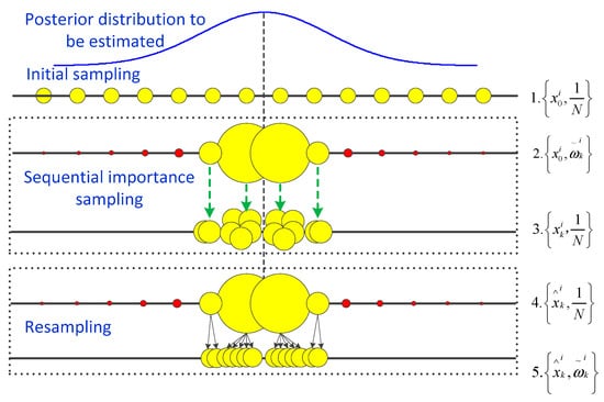
Figure 1.
Schematic diagram of particle filter frame (PFF).
3.3. LRD Predicting Operator Driven by Particle Filter Frame
The flow chart of the degradation trend prognostics for the rolling bearings based on the proposed method is illustrated in Figure 2. The main procedures of the degradation trend prognostics can be described as follows:
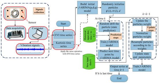
Figure 2.
The flow chart of the proposed method for degeneration trend prognostics of rotating machinery.
- Step 1.
- Particle initialization.
- (a)
- The f-ARIMA degradation models are established by the tested EVI time series or kurtosis time series. In this stage, the initial f-ARIMA model order and coefficients distribution are determined, i.e., , where p and q are model orders, d0 is initial fractional value, and ϕ(i) and θ(i) are model coefficients.
- (b)
- By drifting all of the coefficients set randomly, that is, , where is noise sequence, then the particles set is obtained, the number of particles set is N, and their weights are initialized as .
- Step 2.
- For k = 1, 2, …, L (L is step length):
- (a)
- For k = k − 1, predict the time series output one-step by f-ARIMA model with the parameters .
- (b)
- When the new output time series point yk arrives, update each particle’s weight: .
- (c)
- Normalize the particles weight, i.e., .
- (d)
- Resampling is performed to remove the small weight particles and generate promising new particles with the larger weight, thus the new particles set is .
- Step 3.
- The state vector can be estimated as .
- Step 4.
- Train the f-ARIMA model using the update state vector to get the prediction value of .
- Step 5.
- Algorithm stops when k is equal to step length L, otherwise, go to step (2).
4. Experimental Evaluations
4.1. Experimental Setup
The experimental data were acquired by the Center for Intelligent Maintenance Systems (IMS) [28,29]. The experimental setup and its schematic diagram are displayed in Figure 3a,b, respectively. The vibration acceleration signals were collected every 10 min while input shaft speed was 2000 rpm (33.33 Hz) and the sampling frequency was 20 kHz. Two kinds of accelerated life test experiments were investigated: (1) the first test was carried out successively for 34 days (about 21,560 min), and (2) the second test was carried out successively for 8 days (about 9840 min). In this experiment, the severe wear failure in the inner race of bearing 3 and severe wear failure in the outer race of bearing 1 were respectively detected after dismantling. More details about the experimental description and experiment parameters can be found at the following website: http://www.imscenter.net/.
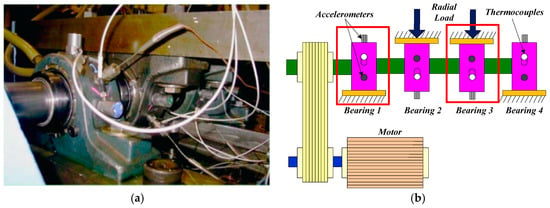
Figure 3.
Experimental setup. (a) Physical experimental platform; (b) Schematic diagram [28,29].
The health indicators time series; i.e., the EVI degeneration curve of bearing 3, and the Kurtosis degeneration curve of bearing 1—are illustrated in Figure 4a,b, respectively. The detailed calculation process of health indicator EVI can be found in ref. [15]. The kurtosis waveform presented in Figure 4b can be divided into running status based on vibration amplitude; i.e., (1) normal operation, (2) incipient fault, and (3) severe fault status. It also should be noted in Figure 6b that some sharp transition points (STPs) are displayed in the incipient and severe fault stages of bearing 1 degeneration.
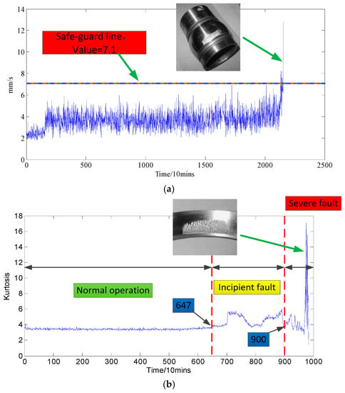
Figure 4.
The equivalent vibration intensity (EVI) curve and kurtosis curve of the bearing degeneration. (a) EVI curve of rolling bearing 3; (b) kurtosis curve of rolling bearing 1.
To demonstrate the validity and superiority of the proposed approach, the EVI and kurtosis degeneration curves are presented as test cases. As a first test case, the EVI time series with weak LRD property has been measured. The second test case is a kurtosis time series with some STPs. Meanwhile, some state-of-the-art prediction methods including the ARMA and FOC methods (f-ARIMA model [15] and FBM model [16]) are also employed for comparison.
4.2. Case 1: The EVI Time Series with Weak LRD Property
Figure 5a shows the EVI curve of bearing 3, from the 801st-point to 1200th-point. The Hurst exponent is calculated via the R/S approach, as shown in Figure 5b. For the time series X(t), the R/S statistic can be expressed by,
where S(n) is the standard deviation (SD); i.e., , and R(n) is the range in each segment. The Hurst H can be generated from the fitted straight line of vs. . The resulting H = 0.5455 is close to 0.5, thus the fractional differencing parameter d = H − 0.5 = 0.0455 > 0 indicates that the EVI time series is to conform to the long-range dependence property. However, the LRD feature is very weak, that is to say, the performance in the future degradation trend has equal probability to be below and above the performance in the current degradation trend. Usually, the prediction accuracy generated by the FOC models may be decreased greatly in this case [13,14,16]. Further, the EVI prognostic result with the proposed method will be described and the results are also compared with the classical ARMA, f-ARIMA, and FBM models.
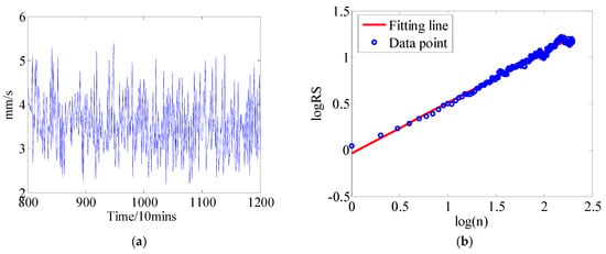
Figure 5.
Weak long-range dependence (LRD) characteristic time series and its Hurst curve. (a) Weak LRD characteristic time series; (b) Hurst curve.
Initially, the LRD model (e.g., f-ARIMA) is defined as , the particular modeling process can refer to [15,30,31], the AR coefficients ϕ(1), ϕ(2), ϕ(3), …, ϕ(p), MA coefficients θ(1), θ(2), θ(3), …, θ(q), wherein the parameters p and q can be calculated by the Akaike information criterion (AIC) [32,33]. The AR coefficients, MA coefficients, and the fractional differencing parameter d are modeled as probability distributions following a certain distribution (called particles). The initial distribution of model parameters can determine the performance of sequential importance sampling (SIS) of PFF. In the update stage, the unknown parameters combined with the state transition probability p(xk|xk−1) can be estimated recursively. Once the update measurements stop, the posterior distribution function p(xk+l|xk) can be calculated to predict a one-step ahead EVI time series based on the latest updated parameters distribution. Furthermore, multi-step (here the step length is L = 40) ahead prognostics can be obtained by performing the prediction process in Bayesian inference. In this experiment, the proposed model is applied to predict 40 points vibration intensity ahead; i.e., 400 min in advance.
The EVI prediction results and errors generated by the proposed method and the ARMA and FOC methods are shown in Figure 6, using the 400 EVI points (from the 801st point to 1200th point) as the historical-based data. The results indicate that the ARMA, f-ARIMA and FBM models cannot generally track the EVI fluctuation trend well under the time series with weak LRD property. As shown in Figure 6d,e, the predicted EVI time series fit the actual time series better than the ARMA, f-ARIMA, and FBM models. It can be seen from Figure 6d,e that, compared with the ARMA and FOC methods, the EVI predictions by the proposed method are closer to the actual values, the prediction results having smaller error values. The specific parameters for quantitative assessment can be found in Table A1 in Appendix A.
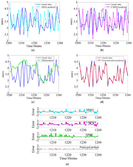
Figure 6.
The EVI prediction results by the proposed method and the other state-of-the-art methods. (a) Prediction result using the autoregressive–moving-average (ARMA) model; (b) Prediction result using the fractionally autoregressive integrated moving average (f-ARIMA) model; (c) Prediction result using the fractional Brownian motion (FBM) model; (d) Prediction result using the proposed model; (e) Prognostic errors.
4.3. Case 2: The Kurtosis Time Series with STPs
Figure 7a shows the kurtosis curve bearing 1 at incipient fault stage, from the 546th point to 945th point. The Hurst exponent is also computed via the R/S approach, as shown in Figure 7b. The resulting H = 0.9640, which is much larger than 0.5, and d = H − 0.5 = 0.4640 indicates that the kurtosis time series have a strong LRD property. However, it should be noted that some STPs are contained in this kurtosis time series (here is historical region, which means the region is formed by the points 546th to point 945th), which illustrates the uncertainties of the predicted data.
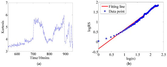
Figure 7.
Kurtosis time series and its Hurst curve. (a) kurtosis time series with sharp transition points; (b) Hurst curve.
In this experiment, 400 kurtosis points (from the 546th point to 945th point) are used as the historical-based data to predict the 40 points; i.e., 400 mins in advance. The prognostic results and prognostic errors with the proposed method and other methods are displayed in Figure 8. It is observed that the prediction values by the f-ARIMA and FBM models gradually deviate from the actual values, especially in the last 15 points (some STPs are contained in the predicted region), which shows that the FOC models have failed when the STPs are contained in the predicted region. By comparison, the proposed approach performs better in multi-step prediction than the existent ARMA model and the FOC models. The specific parameters for quantitative assessment can be found in Table A2 in Appendix A. Overall, the above experimental results verify that the improvement of the proposed approach in terms of the weak-LRD property and STPs time series, which is able to provide a more accurate prediction for the rolling bearing degeneration.
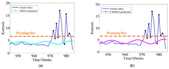
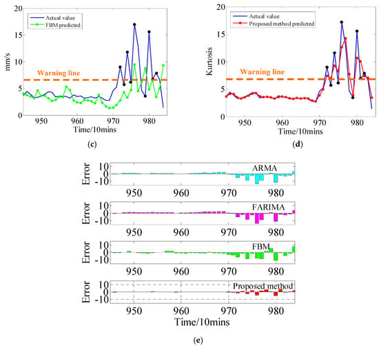
Figure 8.
The kurtosis prediction results by the proposed method and the other state-of-the-art methods. (a) Prediction result using the ARMA model; (b) Prediction result using the f-ARIMA model; (c) Prediction result using the FBM model; (d) Prediction result using the proposed model; (e) Prognostic errors.
5. Conclusions
This paper proposes a novel prognosis approach for the degradation trend of rotating machinery based on a long-range dependence and particle filter algorithm. The main objective is to address the problem of prognostics in FOC models while health indicators time series possess a weak LRD property and the STPs are contained in the predicted range. The two main contributions of this work can be summarized as:
- (1)
- For engineering applications, a new condition prognostic method is introduced as an effective tool for the long lifetime prediction and assessment of mechanical equipment in the PHM filed, the mechanical running degradation pattern can be predicted well in real-time and the most vital components of the mechanical equipment can be repaired and replaced prior to actual catastrophic failure.
- (2)
- For theoretical analysis, the particle filter frame (PFF) is embedded in the FOC model, an update scheme for online model parameters has been introduced to adapt the initial state model based on the PFF algorithm. Due to the adaptability of the parameters, the performance of our proposed model is remarkably efficient than classical time-series ARMA model and the FOC models, even the initial health status is unknown and the failure degradation behavior is time-varying. That is to say, the main advantage of the proposed approach is that the prognostic model has an ability to generate the reliable probabilistic results despite the uncertainties of the initial model parameters.
As we all known, in the case of offline, the vibration data has been collected for further analysis (e.g., trend prediction or remaining useful life, i.e., RUL), and many adaptive prediction methods (such as Wavelet neural network (WNN) and ARMA-recursive least squares, i.e., ARMA-RLS, etc.) with parameters adjustment strategy can be performed only under the known data. Thus, the forecast errors are adjusted based on the predicted data and original data. If the original data is known before the prediction the adaptive prediction methods can work well, but in most cases, the original data is unknown, especially when the equipment is working under normal conditions, so the parameters adjustment strategy does not make sense. Based on this principle, if the original data is unknown, the proposed model is actually able to correctly identify when the bearing lifetime will enter the incipient fault region based on the data from the normal operational region. If not, the proposed model may lose its function.
Future research will investigate the suitability of the proposed model under harsh working conditions or different operational conditions, and the prediction for the remaining useful life (RUL) of the bearing will be investigated. As well, the proposed model might be expanded to other complex industrial applications such as diesel engine failure degradation and aero-engine fault monitor, etc.
Author Contributions
Algorithm improvement, programming and analysis, paper writing was done by Q.L. Review and suggestions were provided by S.Y.L. All authors have read and approved the final manuscript.
Acknowledgments
This research is funded by the Fundamental Research Funds for the Central Universities (Grant No. CUSF-DH-D-2017059 and BCZD2018013) and the Research Funds of Worldtech Transmission Technology (Grant No. 12966EM).
Conflicts of Interest
The authors declare no conflict of interest.
Appendix A

Table A1.
Predicting results using different quantitative parameters for case 1 (The EVI time series with weak LRD property).
Table A1.
Predicting results using different quantitative parameters for case 1 (The EVI time series with weak LRD property).
| Real | ARMA | Error | RE | FARIMA | Error | RE | FBM | Error | RE | Proposed | Error | RE |
|---|---|---|---|---|---|---|---|---|---|---|---|---|
| 4.5522 | 4.851179 | 0.298979 | 0.065678 | 4.315315 | −0.23689 | 0.052038 | 3.692463 | −0.85974 | 0.188862 | 4.338669 | −0.21353 | 0.046907 |
| 3.6649 | 2.928812 | −0.73609 | 0.200848 | 3.116309 | −0.54859 | 0.149688 | 3.829959 | 0.165059 | 0.045038 | 3.754522 | 0.089622 | 0.024454 |
| 3.036 | 3.122478 | 0.086478 | 0.028484 | 2.500855 | −0.53514 | 0.176266 | 4.138178 | 1.102178 | 0.363036 | 3.1013 | 0.0653 | 0.021508 |
| 3.3038 | 4.012963 | 0.709163 | 0.214651 | 4.443229 | 1.139429 | 0.344884 | 4.036887 | 0.733087 | 0.221892 | 3.262692 | −0.04111 | 0.012443 |
| 2.8203 | 3.032396 | 0.212096 | 0.075203 | 3.228642 | 0.408342 | 0.144787 | 3.947579 | 1.127279 | 0.399702 | 2.87064 | 0.05034 | 0.017849 |
| 3.2525 | 3.090151 | −0.16235 | 0.049915 | 3.305279 | 0.052779 | 0.016227 | 4.043051 | 0.790551 | 0.243059 | 3.19275 | −0.05975 | 0.018371 |
| 4.1008 | 3.887408 | −0.21339 | 0.052037 | 3.536877 | −0.56392 | 0.137515 | 3.998855 | −0.10194 | 0.02486 | 3.985144 | −0.11566 | 0.028203 |
| 3.2772 | 4.359959 | 1.082759 | 0.330391 | 4.294689 | 1.017489 | 0.310475 | 4.301419 | 1.024219 | 0.312529 | 3.362803 | 0.085603 | 0.026121 |
| 2.4798 | 3.038506 | 0.558706 | 0.225303 | 3.073638 | 0.593838 | 0.23947 | 4.407019 | 1.927219 | 0.777167 | 2.569523 | 0.089723 | 0.036181 |
| 3.9129 | 4.451459 | 0.538559 | 0.137637 | 4.483454 | 0.570554 | 0.145814 | 4.465283 | 0.552383 | 0.14117 | 3.731065 | −0.18184 | 0.046471 |
| 4.5876 | 3.712715 | −0.87489 | 0.190707 | 4.176524 | −0.41108 | 0.089606 | 4.436422 | −0.15118 | 0.032954 | 4.487611 | −0.09999 | 0.021795 |
| 2.4631 | 2.732075 | 0.268975 | 0.109202 | 2.190463 | −0.27264 | 0.110689 | 4.635023 | 2.171923 | 0.881784 | 2.706797 | 0.243697 | 0.098939 |
| 4.55 | 4.025714 | −0.52429 | 0.115228 | 4.073607 | −0.47639 | 0.104702 | 4.550027 | 2.66×10⁻⁵ | 5.84×10⁻⁶ | 4.286559 | −0.26344 | 0.057899 |
| 4.146 | 3.494402 | −0.6516 | 0.157163 | 3.316627 | −0.82937 | 0.200042 | 4.588838 | 0.442838 | 0.106811 | 4.175007 | 0.029007 | 0.006996 |
| 2.7487 | 2.343199 | −0.4055 | 0.147525 | 2.717725 | −0.03097 | 0.011269 | 4.165975 | 1.417275 | 0.515617 | 2.905444 | 0.156744 | 0.057025 |
| 3.0865 | 3.63355 | 0.54705 | 0.17724 | 3.757182 | 0.670682 | 0.217295 | 4.169485 | 1.082985 | 0.350878 | 3.03899 | −0.04751 | 0.015393 |
| 4.1998 | 3.571195 | −0.62861 | 0.149675 | 3.843438 | −0.35636 | 0.084852 | 4.076447 | −0.12335 | 0.029371 | 4.052326 | −0.14747 | 0.035115 |
| 3.1988 | 3.510075 | 0.311275 | 0.09731 | 3.290616 | 0.091816 | 0.028703 | 3.958997 | 0.760197 | 0.237651 | 3.30548 | 0.10668 | 0.03335 |
| 3.0569 | 4.620933 | 1.564033 | 0.51164 | 4.349495 | 1.292595 | 0.422845 | 4.201031 | 1.144131 | 0.374278 | 3.065222 | 0.008322 | 0.002722 |
| 3.8719 | 4.094481 | 0.222581 | 0.057486 | 4.475258 | 0.603358 | 0.15583 | 4.209925 | 0.338025 | 0.087302 | 3.761908 | −0.10999 | 0.028408 |
| 3.5429 | 3.102141 | −0.44076 | 0.124406 | 2.865971 | −0.67693 | 0.191066 | 4.244785 | 0.701885 | 0.19811 | 3.568503 | 0.025603 | 0.007227 |
| 4.4554 | 3.754243 | −0.70116 | 0.157372 | 4.179654 | −0.27575 | 0.06189 | 4.216189 | −0.23921 | 0.05369 | 4.328812 | −0.12659 | 0.028412 |
| 4.2155 | 3.506033 | −0.70947 | 0.1683 | 3.196617 | −1.01888 | 0.241699 | 3.419768 | −0.79573 | 0.188763 | 4.224678 | 0.009178 | 0.002177 |
| 2.521 | 2.621368 | 0.100368 | 0.039813 | 2.579941 | 0.058941 | 0.02338 | 3.423397 | 0.902397 | 0.357952 | 2.714081 | 0.193081 | 0.076589 |
| 3.2362 | 4.057441 | 0.821241 | 0.253767 | 3.836757 | 0.600557 | 0.185575 | 3.377986 | 0.141786 | 0.043813 | 3.143407 | −0.09279 | 0.028673 |
| 3.1059 | 3.091177 | −0.01472 | 0.00474 | 3.682622 | 0.576722 | 0.185686 | 3.026959 | −0.07894 | 0.025416 | 3.112301 | 0.006401 | 0.002061 |
| 2.9839 | 2.908971 | −0.07493 | 0.025111 | 2.831969 | −0.15193 | 0.050917 | 2.832535 | −0.15137 | 0.050727 | 2.990418 | 0.006518 | 0.002184 |
| 2.7785 | 4.240453 | 1.461953 | 0.526166 | 4.188664 | 1.410164 | 0.507527 | 2.850715 | 0.072215 | 0.025991 | 2.796518 | 0.018018 | 0.006485 |
| 3.3918 | 3.682935 | 0.291135 | 0.085835 | 3.509299 | 0.117499 | 0.034642 | 3.124385 | −0.26741 | 0.078842 | 3.309347 | −0.08245 | 0.02431 |
| 3.0046 | 3.348826 | 0.344226 | 0.114566 | 3.001548 | −0.00305 | 0.001016 | 2.957211 | −0.04739 | 0.015772 | 3.041626 | 0.037026 | 0.012323 |
| 3.0101 | 4.347179 | 1.337079 | 0.444197 | 4.64161 | 1.63151 | 0.542012 | 3.099322 | 0.089222 | 0.029641 | 3.001522 | −0.00858 | 0.00285 |
| 4.226 | 3.36362 | −0.86238 | 0.204065 | 3.548991 | −0.67701 | 0.160201 | 3.639928 | −0.58607 | 0.138682 | 4.066107 | −0.15989 | 0.037836 |
| 2.9203 | 2.747795 | −0.1725 | 0.059071 | 2.890067 | −0.03023 | 0.010353 | 3.486781 | 0.566481 | 0.19398 | 3.064534 | 0.144234 | 0.04939 |
| 3.9785 | 4.071772 | 0.093272 | 0.023444 | 3.644438 | −0.33406 | 0.083967 | 3.687806 | −0.29069 | 0.073066 | 3.839084 | −0.13942 | 0.035042 |
| 2.8849 | 3.696822 | 0.811922 | 0.281438 | 3.812164 | 0.927264 | 0.32142 | 3.740511 | 0.855611 | 0.296583 | 3.004821 | 0.119921 | 0.041569 |
| 2.781 | 2.821017 | 0.040017 | 0.014389 | 2.481329 | −0.29967 | 0.107757 | 4.339559 | 1.558559 | 0.560431 | 2.787078 | 0.006078 | 0.002185 |
| 3.8017 | 4.081894 | 0.280194 | 0.073702 | 4.310372 | 0.508672 | 0.133801 | 4.144882 | 0.343182 | 0.090271 | 3.668168 | −0.13353 | 0.035124 |
| 4.6639 | 3.529533 | −1.13437 | 0.243223 | 3.672363 | −0.99154 | 0.212598 | 4.21923 | −0.44467 | 0.095343 | 4.540967 | −0.12293 | 0.026358 |
| 3.8834 | 2.812674 | −1.07073 | 0.275719 | 2.667587 | −1.21581 | 0.313079 | 4.152104 | 0.268704 | 0.069193 | 3.957954 | 0.074554 | 0.019198 |
| 3.3754 | 4.384567 | 1.009167 | 0.298977 | 4.223374 | 0.847974 | 0.251222 | 4.010072 | 0.634672 | 0.188029 | 3.422911 | 0.047511 | 0.014076 |
Note that: .

Table A2.
Predicting results using different quantitative parameters for case 2 (The Kurtosis time series with STPs).
Table A2.
Predicting results using different quantitative parameters for case 2 (The Kurtosis time series with STPs).
| Real | ARMA | Error | RE | FARIMA | Error | RE | FBM | Error | RE | Proposed | Error | RE |
|---|---|---|---|---|---|---|---|---|---|---|---|---|
| 3.643158 | 3.583676 | −0.05948 | 0.016327 | 3.573756 | −0.0694 | 0.01905 | 4.032532 | 0.389374 | 0.106878 | 3.658809 | 0.015651 | 0.004296 |
| 4.458712 | 3.72162 | −0.73709 | 0.165315 | 3.698368 | −0.76034 | 0.17053 | 3.767629 | −0.69108 | 0.154996 | 4.125354 | −0.33336 | 0.074765 |
| 3.885578 | 3.867426 | −0.01815 | 0.004672 | 3.848826 | −0.03675 | 0.009459 | 3.486229 | −0.39935 | 0.102777 | 4.097066 | 0.211488 | 0.054429 |
| 3.26448 | 4.058685 | 0.794206 | 0.243287 | 4.109618 | 0.845139 | 0.258889 | 3.156036 | −0.10844 | 0.033219 | 3.507751 | 0.243271 | 0.074521 |
| 3.326908 | 4.248171 | 0.921263 | 0.276913 | 4.428144 | 1.101236 | 0.331009 | 4.602094 | 1.275186 | 0.383295 | 3.306727 | −0.02018 | 0.006066 |
| 3.596278 | 4.40949 | 0.813212 | 0.226126 | 4.669793 | 1.073515 | 0.298507 | 3.575741 | −0.02054 | 0.005711 | 3.490924 | −0.10535 | 0.029295 |
| 3.911841 | 4.51446 | 0.602619 | 0.15405 | 4.809623 | 0.897783 | 0.229504 | 3.624969 | −0.28687 | 0.073334 | 3.781957 | −0.12988 | 0.033203 |
| 4.374046 | 4.545397 | 0.171351 | 0.039175 | 4.892967 | 0.518921 | 0.118636 | 3.181498 | −1.19255 | 0.272642 | 4.17795 | −0.1961 | 0.044832 |
| 4.252138 | 4.496206 | 0.244068 | 0.057399 | 4.834369 | 0.582232 | 0.136927 | 2.674354 | −1.57778 | 0.371057 | 4.28264 | 0.030502 | 0.007173 |
| 3.393007 | 4.374221 | 0.981215 | 0.289187 | 4.699951 | 1.306944 | 0.385188 | 2.841052 | −0.55195 | 0.162674 | 3.724723 | 0.331716 | 0.097765 |
| 3.612475 | 4.199098 | 0.586623 | 0.162388 | 4.481938 | 0.869463 | 0.240683 | 3.447842 | −0.16463 | 0.045574 | 3.52586 | −0.08662 | 0.023977 |
| 3.561138 | 3.999812 | 0.438674 | 0.123184 | 4.222849 | 0.661711 | 0.185815 | 3.387714 | −0.17342 | 0.048699 | 3.579461 | 0.018323 | 0.005145 |
| 3.465567 | 3.809977 | 0.34441 | 0.099381 | 3.963394 | 0.497827 | 0.14365 | 5.315971 | 1.850404 | 0.53394 | 3.502904 | 0.037337 | 0.010774 |
| 3.168745 | 3.662308 | 0.493563 | 0.15576 | 3.700369 | 0.531624 | 0.167771 | 4.683602 | 1.514857 | 0.478062 | 3.289646 | 0.120902 | 0.038154 |
| 3.819911 | 3.583102 | −0.23681 | 0.061993 | 3.562851 | −0.25706 | 0.067295 | 2.746134 | −1.07378 | 0.2811 | 3.56325 | −0.25666 | 0.06719 |
| 3.500932 | 3.587702 | 0.08677 | 0.024785 | 3.53361 | 0.032678 | 0.009334 | 2.37261 | −1.12832 | 0.322292 | 3.623144 | 0.122212 | 0.034908 |
| 3.570946 | 3.677685 | 0.106739 | 0.029891 | 3.616021 | 0.045075 | 0.012623 | 2.29524 | −1.27571 | 0.357246 | 3.54248 | −0.02847 | 0.007972 |
| 3.168281 | 3.840316 | 0.672035 | 0.212113 | 3.826746 | 0.658465 | 0.20783 | 2.838346 | −0.32994 | 0.104137 | 3.329741 | 0.16146 | 0.050961 |
| 3.293096 | 4.05039 | 0.757294 | 0.229964 | 4.099097 | 0.806001 | 0.244755 | 2.776671 | −0.51643 | 0.156821 | 3.249593 | −0.0435 | 0.01321 |
| 3.446315 | 4.274201 | 0.827886 | 0.240224 | 4.429192 | 0.982877 | 0.285197 | 2.604462 | −0.84185 | 0.244276 | 3.388605 | −0.05771 | 0.016745 |
| 3.162353 | 4.475022 | 1.312669 | 0.415092 | 4.722749 | 1.560396 | 0.493429 | 2.233966 | −0.92839 | 0.293575 | 3.278397 | 0.116044 | 0.036696 |
| 3.466872 | 4.619211 | 1.152339 | 0.332386 | 4.955867 | 1.488995 | 0.429492 | 3.825701 | 0.358829 | 0.103502 | 3.350685 | −0.11619 | 0.033513 |
| 3.173705 | 4.68192 | 1.508215 | 0.475222 | 5.108123 | 1.934418 | 0.609514 | 2.313129 | −0.86058 | 0.271158 | 3.293016 | 0.119311 | 0.037594 |
| 2.735459 | 4.651447 | 1.915989 | 0.700427 | 5.101645 | 2.366186 | 0.865005 | 1.647156 | −1.0883 | 0.39785 | 2.919846 | 0.184387 | 0.067406 |
| 2.741126 | 4.531477 | 1.790351 | 0.653145 | 4.975918 | 2.234792 | 0.815283 | 1.354652 | −1.38647 | 0.505804 | 2.755165 | 0.014039 | 0.005121 |
| 4.596144 | 4.340782 | −0.25536 | 0.05556 | 4.725386 | 0.129242 | 0.02812 | 1.409942 | −3.1862 | 0.693234 | 3.86102 | −0.73512 | 0.159944 |
| 5.237255 | 4.110381 | −1.12687 | 0.215165 | 4.39778 | −0.83947 | 0.160289 | 1.939538 | −3.29772 | 0.629665 | 4.953759 | −0.2835 | 0.054131 |
| 9.022867 | 3.878593 | −5.14427 | 0.570137 | 4.052994 | −4.96987 | 0.550809 | 2.780149 | −6.24272 | 0.691877 | 7.451932 | −1.57093 | 0.174106 |
| 5.710835 | 3.684756 | −2.02608 | 0.354778 | 3.721233 | −1.9896 | 0.348391 | 4.30398 | −1.40685 | 0.246348 | 6.932928 | 1.222093 | 0.213995 |
| 11.78736 | 3.562644 | −8.22472 | 0.697757 | 3.501299 | −8.28607 | 0.702962 | 3.285498 | −8.50187 | 0.72127 | 9.278318 | −2.50905 | 0.212859 |
| 6.161553 | 3.534682 | −2.62687 | 0.426333 | 3.397958 | −2.7636 | 0.448522 | 4.699429 | −1.46212 | 0.237298 | 8.261117 | 2.099564 | 0.340752 |
| 17.11001 | 3.607951 | −13.5021 | 0.789132 | 3.439155 | −13.6709 | 0.798997 | 9.469801 | −7.64021 | 0.446534 | 12.61797 | −4.49204 | 0.262538 |
| 12.79646 | 3.772676 | −9.02378 | 0.705178 | 3.639572 | −9.15689 | 0.71558 | 4.514397 | −8.28206 | 0.647215 | 14.24967 | 1.453207 | 0.113563 |
| 4.624278 | 4.003519 | −0.62076 | 0.134239 | 3.945269 | −0.67901 | 0.146836 | 6.213077 | 1.588799 | 0.343578 | 7.733383 | 3.109106 | 0.672344 |
| 3.468857 | 4.263509 | 0.794651 | 0.229082 | 4.336045 | 0.867188 | 0.249992 | 8.735766 | 5.266909 | 1.518341 | 3.912321 | 0.443463 | 0.127841 |
| 15.5777 | 4.510005 | −11.0677 | 0.710483 | 4.723523 | −10.8542 | 0.696777 | 4.796129 | −10.7816 | 0.692116 | 10.67374 | −4.90396 | 0.314806 |
| 6.759972 | 4.701735 | −2.05824 | 0.304474 | 5.057507 | −1.70246 | 0.251845 | 6.469648 | −0.29032 | 0.042947 | 10.07051 | 3.310534 | 0.489726 |
| 7.891755 | 4.805755 | −3.086 | 0.391041 | 5.288081 | −2.60367 | 0.329923 | 3.409635 | −4.48212 | 0.56795 | 7.36274 | −0.52901 | 0.067034 |
| 6.637513 | 4.803148 | −1.83437 | 0.276363 | 5.347143 | −1.29037 | 0.194406 | 4.985756 | −1.65176 | 0.248852 | 7.050467 | 0.412954 | 0.062215 |
| 1.390226 | 4.692493 | 3.302267 | 2.375345 | 5.250833 | 3.860607 | 2.776964 | 9.331603 | 7.941377 | 5.712292 | 3.44751 | 2.057284 | 1.47982 |
Note that: .
References
- Lee, J.; Wu, F.J.; Zhao, W.Y.; Ghaffari, M.; Liao, L.X.; Siegel, D. Prognostics and health management design for rotary machinery systems-Reviews, methodology and applications. Mech. Syst. Signal Process. 2014, 42, 314–334. [Google Scholar] [CrossRef]
- Li, Y.; Kurfess, T.R.; Liang, S.Y. Stochastic prognostic for rolling element bearings. Mech. Syst. Signal Process. 2000, 14, 747–762. [Google Scholar] [CrossRef]
- Chen, Z.S.; Yang, Y.M.; Hu, Z. A technical framework and roadmap of embedded diagnostics and prognostics for complex mechanical systems in prognostics and health management systems. IEEE Trans. Reliab. 2012, 61, 314–322. [Google Scholar] [CrossRef]
- Li, Q.; Liang, S.Y. Incipient fault diagnosis of rolling bearings based on impulse-step impact dictionary and re-weighted minimizing nonconvex penalty Lq regular technique. Entropy 2017, 19, 421. [Google Scholar] [CrossRef]
- Shih, Y.; Chen, J. Analysis of fatigue crack growth on a cracked shaft. Int. J. Fatigue 1997, 19, 477–485. [Google Scholar]
- Choi, Y.; Liu, C. Spall progression life model for rolling contact verified by finish hard machined surfaces. Wear 2007, 262, 24–35. [Google Scholar] [CrossRef]
- Samah, A.A.; Shahzad, M.K.; Zamai, E. Bayesian based methodology for the extraction and validation of time bound failure signatures for online failure prediction. Reliab. Eng. Syst. Safe 2017, 167, 616–628. [Google Scholar] [CrossRef]
- Chetouani, Y. Model selection and fault detection approach based on Bayes decision theory: Application to changes detection problem in a distillation column. Process. Saf. Environ. 2014, 92, 215–223. [Google Scholar] [CrossRef]
- Ren, L.; Cui, J.; Sun, Y.Q.; Cheng, X.J. Multi-bearing remaining useful life collaborative prediction: A deep learning approach. J. Manuf. Syst. 2017, 43, 248–256. [Google Scholar] [CrossRef]
- Mao, W.T.; He, L.; Yan, Y.J.; Wang, J.W. Online sequential prediction of bearings imbalanced fault diagnosis by extreme learning machine. Mech. Syst. Signal Process. 2017, 83, 450–473. [Google Scholar] [CrossRef]
- Gangsar, P.; Tiwari, R. Comparative investigation of vibration and current monitoring for prediction of mechanical and electrical faults in induction motor based on multiclass-support vector machine algorithms. Mech. Syst. Signal Process. 2017, 94, 464–481. [Google Scholar] [CrossRef]
- Hou, S.M.; Li, Y.R. Short-term fault prediction based on support vector machines with parameter optimization by evolution strategy. Expert. Syst. Appl. 2009, 36, 12383–12391. [Google Scholar] [CrossRef]
- Li, M.; Li, J.Y. Generalized Cauchy model of sea level fluctuations with long-range dependence. Physica A 2017, 484, 309–335. [Google Scholar] [CrossRef]
- Li, M.; Li, J.Y. On the predictability of long-range dependent series. Math. Probl. Eng. 2010, 2010, 397454. [Google Scholar] [CrossRef]
- Li, Q.; Liang, S.Y.; Yang, J.G.; Li, B.Z. Long range dependence prognostics for bearing vibration intensity chaotic time series. Entropy 2016, 18, 23. [Google Scholar] [CrossRef]
- Li, Q.; Liang, S.Y. Degradation trend prognostics for rolling bearing using improved R/S statistic model and fractional Brownian motion approach. IEEE Access 2017, 99, 21103–21114. [Google Scholar] [CrossRef]
- Song, W.Q.; Li, M.; Liang, J.K. Prediction of bearing fault using fractional Brownian motion and minimum entropy deconvolution. Entropy 2016, 18, 418. [Google Scholar] [CrossRef]
- Mandelbrot, B.B.; Ness, J.W.V. Fractional Brownian motions, fractional noises and applications. SIAM Rev. 1968, 10, 422–437. [Google Scholar] [CrossRef]
- Li, M. Fractional gaussian noise and network traffic modeling. In Proceedings of the 8th WSEAS International Conference on Applied Computer and Applied Computational Science, Canary Islands, Spain, 14–16 December 2009; Volume 34, p. 39. [Google Scholar]
- Beran, J.; Feng, Y.; Ghosh, S.; Kulik, R. Long-Memory Processes-Probabilistic Properties and Statistical Methods; Springer: London, UK, 2013. [Google Scholar]
- Hosking, J.R.M. Fractional differencing. Biometrika 1981, 68, 165–176. [Google Scholar] [CrossRef]
- Kavasseri, R.G.; Seetharaman, K. Day-ahead wind speed forecasting using f-ARIMA models. Renew. Energy 2009, 34, 1388–1393. [Google Scholar] [CrossRef]
- Beran, J. Statistics for Long-Memory Processes; Chapman and Hall: New York, NY, USA, 1994. [Google Scholar]
- Taqqu, M.S.; Teverovsky, V. On estimating the intensity of long-range dependence in finite and infinite variance time series. In A Practical Guide to Heavy Tails: Statistical Techniques and Applications; Birkhauser Boston Inc.: Cambridge, MA, USA, 1998; pp. 177–217. [Google Scholar]
- Arulampalam, M.S.; Maskell, S.; Gordon, N.; Clapp, T. A tutorial on particle filters for online nonlinear/non-Gaussian Bayesian tracking. IEEE Trans. Signal Process. 2002, 50, 174–188. [Google Scholar] [CrossRef]
- Doucet, A.; Freitas, N.D.; Gordon, N. Sequential Monte Carlo Methods in Practice; Springer: New York, NY, USA, 2001. [Google Scholar]
- Wang, P.; Gao, R.X. Adaptive resampling-based particle filtering for tool life prediction. J. Manuf. Syst. 2015, 37, 528–534. [Google Scholar] [CrossRef]
- Center for Intelligent Maintenance Systems. Available online: http://www.imscenter.net/ (accessed on 14 January 2018).
- Qiu, H.; Lee, J.; Lin, J.; Yu, G. Wavelet filter-based weak signature detection method and its application on roller bearing prognostics. J. Sound Vib. 2006, 289, 1066–1090. [Google Scholar] [CrossRef]
- Yuan, X.H.; Tan, Q.X.; Lei, X.H.; Yuan, Y.B.; Wu, X.T. Wind power prediction using hybrid autoregressive fractionally integrated moving average and least square support vector machine. Energy 2017, 129, 122–137. [Google Scholar] [CrossRef]
- Chu, F.L. A fractionally integrated autoregressive moving average approach to forecasting tourism demand. Tour. Manag. 2008, 29, 79–88. [Google Scholar] [CrossRef]
- Akaike, H. A new look at the statistical model identification. IEEE Trans. Autom. Control 1974, 19, 716–723. [Google Scholar] [CrossRef]
- Akaike, H. Prediction and Entropy; Springer: New York, NY, USA, 1985; pp. 1–24. [Google Scholar]
© 2018 by the authors. Licensee MDPI, Basel, Switzerland. This article is an open access article distributed under the terms and conditions of the Creative Commons Attribution (CC BY) license (http://creativecommons.org/licenses/by/4.0/).