Safe Path Planning of Mobile Robot Based on Improved A* Algorithm in Complex Terrains

Abstract

The A* algorithm has been widely investigated and applied in path planning problems, but it does not fully consider the safety and smoothness of the path. Therefore, an improved A* algorithm is presented in this paper. Firstly, a new environment modeling method is proposed in which the evaluation function of A* algorithm is improved by taking the safety cost into account. This results in a safer path which can stay farther away from obstacles. Then a new path smoothing method is proposed, which introduces a path evaluation mechanism into the smoothing process. This method is then applied to smoothing the path without safety reduction. Secondly, with respect to path planning problems in complex terrains, a complex terrain environment model is established in which the distance and safety cost of the evaluation function of the A* algorithm are converted into time cost. This results in a unification of units as well as a clarity in their physical meanings. The simulation results show that the improved A* algorithm can greatly improve the safety and smoothness of the planned path and the movement time of the robot in complex terrain is greatly reduced.

1. Introduction

Path planning is one of the fundamental problems in robotics [1,2]. It is typically defined as finding a sequence of state transitions for a robot from its initial state to some desired goal state. According to the information of obstacles, the working environment of a robot can be categorized as a completely known environment, a partially known environment, a completely unknown environment, and a dynamic environment [3]. The planned path of the robot can be evaluated according to path length, movement time, energy consumption, or risk level [4,5].

There have been numerous algorithms proposed for path planning of intelligent robots and navigational objects [6], such as the probabilistic roadmap method (PRM) [7], the rapidly exploring random trees algorithm (RRT) [8], the expansive space trees algorithm (EST) [9], the rapidly exploring random trees star (RRT*) algorithm [10], the artificial potential field method (APF) [11,12], the model predictive control method (MPC) [13], fuzzy logic approach [14,15], the artificial neural networks algorithm (ANN) [16], the genetic algorithm (GA) [17], ant colony optimization (ACO) [18,19], particle swarm optimization (PSO) [20], and other new nature-inspired meta-heuristic algorithms [21,22]. Compared to these algorithms, A* algorithm has been widely investigated and applied because of its advantages such as its simple principle, easy realization, high efficiency, and its ability to find the optimal solution. To further increase the applicability of A* algorithm, many scholars have improved the conventional A* algorithm. First, the evaluation function of A* algorithm has been improved so that the planned path can meet specific requirements [23,24,25]. H. Shi et al. [23] took the distance and direction as two heuristic elements of the evaluation function and solved the problem of non-uniform units by normalization; thus, the search efficiency of A* algorithm was improved. Z.Y. Lu et al. [24] introduced the gravity navigation information into the evaluation function so that the improved A* algorithm could enhance the performance of gravity-aided inertial navigation. W. W. Zhan et al. [25] took the flight altitude, detected probability, and flight length into consideration to search for the optimal flight path between two waypoints so that the planned path could be a significant distance away from the danger zone. Second, in the path planning process, the grid states to be expanded are selected based on new rules to improve the search’s efficacy or the path performance [26,27,28]. R. J. Szczerba et al. [26] presented a novel path planning approach called Sparse A* Search; the approach removed the unfeasible search space of the current track point according to the track constraint. As a result, search time was shortened and the memory space was reduced. Y.N. Zhang et al. [27] only selected those neighboring states which satisfy dynamic motion constraints, including maximum turning angle and maximum climb/glide slope angle of the vehicle; thus, the search space was diminished and search efficiency was improved. In Y. Xin et al. [28], the search state was defined as the grid line instead of the grid center; accordingly, the number of searchable neighbor states was extended from eight to infinity. As a result, the planned path was much shorter and the number of turning states was greatly reduced. Third, the path generated by A* algorithm was smoothed to reduce the length, turning times, and turning angle to be more in line with the actual motion requirements of the robot [29,30,31]. H.W. Wang et al. [29] established a smoothing A* model by traversing all the states on initial path planned by A* algorithm and deleting the states which prolonged the length of initial path as no obstacles existing on the line connected by forward and after states. W. Shan et al. [30] applied a key optimization process to simplify the global path, which was planned by the conventional A* algorithm, to be connected among a series of key points. In this process, the polar polynomials curve was introduced to smooth the path according to the constraints of position, curvature, and slope. D. J. Wang et al. [31] simplified the planned path by keeping only the start point, inflection point, and the end point of the path. The rotation direction and the minimum rotation angles at the inflection points were calculated for adjusting the robot’s posture. There have been many other improvements to the conventional A* algorithm, such as the Jump Point Search [32] and hierarchical A* algorithm [33].

The above-mentioned works have enhanced the performance of conventional A* algorithm to some extent. However, the influence of the distance between the robot and obstacles on the safety of the robot has not been fully considered. To avoid a collision between the robot and obstacles, the most common way is to expand the obstacles when establishing an environment model in the grid-based path planning algorithm. The planned path maintains a certain distance to the actual obstacles as he traversing process of path planning does not allow an extension to the states in the expanding obstacles. This method conveniently can establish environment models and simplify algorithm operations; however, in reality, the safety of the robot is not only related to the distances between the robot and any obstacles but also the speed of the robot. The faster the robot moves, the larger a distance should be maintained between the robot and obstacles. The robot could pass through narrow areas where the obstacles are close together safely by reducing speed. A simple expansion of the obstacles may increase the length of the planned path because the obstacle area is increase; moreover, in a complex environment with dense obstacles, expanding obstacles may block the passable areas and lead to the failure of path searching. Juan David Hernández et al. [34] proposed to establish risk zones and direction vectors risk around the vehicle; the RRT* algorithm was then used to search for a feasible and safe path. In this method, the planned path can keep away from obstacles; however, it needs to check for collision for each sampled configuration from the inner to the outer zone as well as the intermediate steps when connecting to others. Accordingly, search efficiency may be decreased. Therefore, a new modeling method is proposed in this paper. The new method does not expand the obstacles; it sets up the weights of the grid states around obstacles according to the distance between the states and obstacles. The weight of a state indicates the safety cost of a robot to pass through; the closer the state and obstacles are, the greater the weight will be. As a result, the planned path would be as far away as possible from the obstacles and the passable areas would not be blocked by expanding obstacles. Moreover, in order to make the planned path more natural and suitable for the robot’s movement, the path is smoothed and a path evaluation mechanism is adopted in the smoothing process to ensure the optimization of the smooth path.

Additionally, the speed of the robot is usually set to be a constant value in a single terrain environment so that the shorter the planned path is, the less time the robot will spend when moving from the initial state to the goal state. However, in a complex terrain environment, the robot would move at different speeds when passing through different terrains, so that the shorter path does not mean less movement time. Therefore, this paper establishes a complex terrain environment model which focuses on the speed and safety of the robot and takes the movement time of the robot as the objective function of A* algorithm for path planning. Then the planned path is smoothed without a decrease in performance.

The rest of this article is organized as follows: Section 2 reviews the conventional A* algorithm. Section 3 presents the improved A* algorithm in detail, including the new environment modeling method and path smoothing operation. Section 4 establishes a complex terrain environment and searches the optimal path by using the improved A* algorithm. Finally, Section 5 gives the conclusions and suggestions.

2. A* Algorithm

A* algorithm is a heuristic search algorithm established on the basis of Dijkstra’s algorithm [35] and the BFS (Breadth First Search) algorithm [36]. The implementation of A* algorithm largely includes environment modeling and optimal path searching; this section illustrates these respectively.

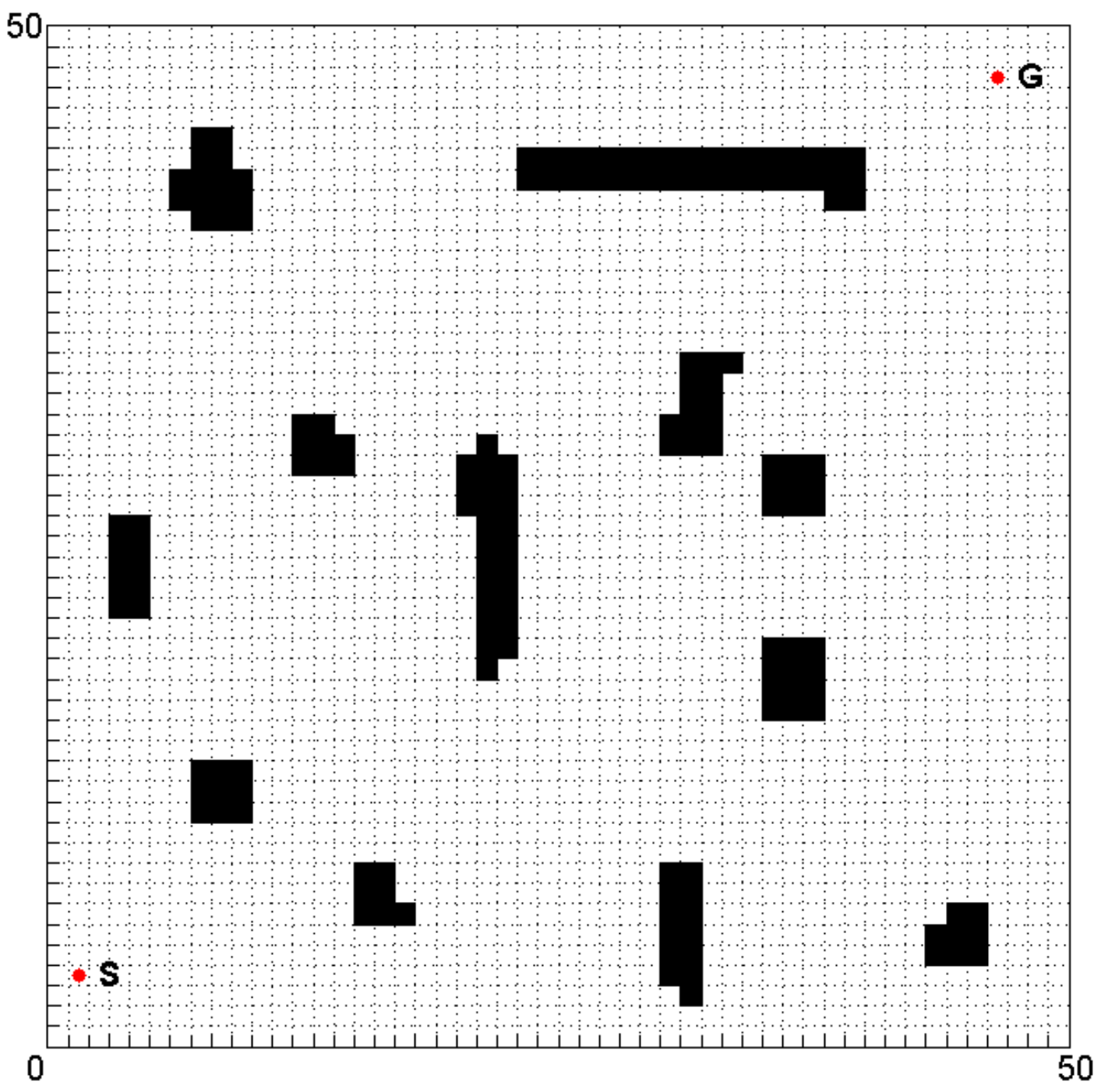
2.1. Environment Model

As A* algorithm is a grid traversal search algorithm, we should first establish the grid model of the environment map by grid method. The grid method divides the map into adjacent grids of equal size. The size of the grid is determined by the size of the robot and it affects the efficiency and searching precision of the algorithm. The grid model of a two-dimensional environment map is as shown in Figure 1.

Figure 1 represents the square with a side of length 50 m; it is divided into 50 × 50 grids. Each grid represents a state where the robot can stay; it is connected to its eight neighbors. The black regions are known obstacle locations while the white regions are locations known to be in free space. The position coordinates of the initial state, S, are (2, 4) and the position coordinates of the goal state, G, are (47, 48). The task of path planning is to find an optimal path that leads the robot from S to G.

2.2. Algorithm Procedures

The focus of A* algorithm is to expand outward from the initial state S, compute the evaluation function value of each neighboring state, and select the state which has the minimum evaluation function value as the next traversal state. It then repeats the expanding process until the goal state G is traversed.

The evaluation function of each state X is defined as follows

f(X) = g(X) + h(X),

(1)

where f(X) denotes the estimated path cost from S through X to G, g(X) denotes the actual path cost from S to X, and h(X) is the heuristic function which denotes the estimated path cost from X to G. The heuristic function is generally expressed as Manhattan distance, diagonal distance, or Euclidean distance. This article adopts diagonal distance as the estimated path cost.

A* algorithm maintains an OPEN list of states for expansion. The OPEN list is used to store states waiting to be traversed. Every state X except S has a hidden arrow pointing to an adjacent state Y denoted by p(X) = Y. A* algorithm uses the arrows to represent the path from X to Y. Every state X has an associated tag t(X) such that t(X) = new if X has never been on the OPEN list, t(X) = open if X is currently on the OPEN list, and t(X) = closed if X is no longer on the OPEN list. The cost of moving from X to a neighboring state Y is a positive number given by the moving cost function c(X, Y). The procedure of A* algorithm is given in Algorithm 1.

Algorithm 1: A*(S, G)

1 for each state X in the environment model: 2  t(X) = new; 3  Initialize the OPEN list to be empty; Place state S on the OPEN list; t(S) = open; g(S) = 0; 4 while t(G) ≠ closed: 5  Find the state, X, on the OPEN list with minimum estimated path cost; 6  for each neighbor Y of X: 7   if Y is not in a forbidden region 8    if t(Y) = new 9     p(Y) = X; g(Y) = g(X) + c(X, Y); f(Y) = g(Y) + h(Y); Place Y on the OPEN list; t(Y) = open; 10    else if t(Y) = open 11     if g(X) + c(X, Y) + h(Y) < f(Y) 12      g(Y) = g(X) + c(X, Y); f(Y) = g(Y) + h(Y); p(Y) = X; 13  Delete X from the OPEN list; t(X) = closed; 14  if OPEN = NULL 15   return NO-PATH; 16 The optimal path from S to G is obtained.

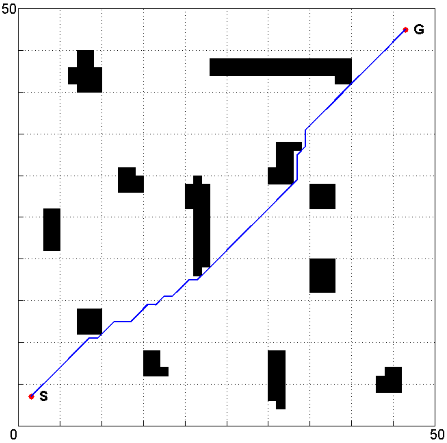
2.3. Algorithm Simulation

According to the procedure of A* algorithm, the simulation experiment of the path planning in the environment model shown in Figure 1 is done by MATLAB R2012a and the result is shown in Figure 2.

It can be seen from Figure 2 that the path generated by the conventional A* algorithm is close to the obstacles and has many turning points; accordingly, it is detrimental to the actual movement of the robot.

3. Improvement of A* Algorithm

In order to increase the safety of the planned path generated by the conventional A* algorithm, a new environment modeling method is proposed and the evaluation function is improved to keep the path away from obstacles. As a result, the safe path is smoothed without decreasing the safety.

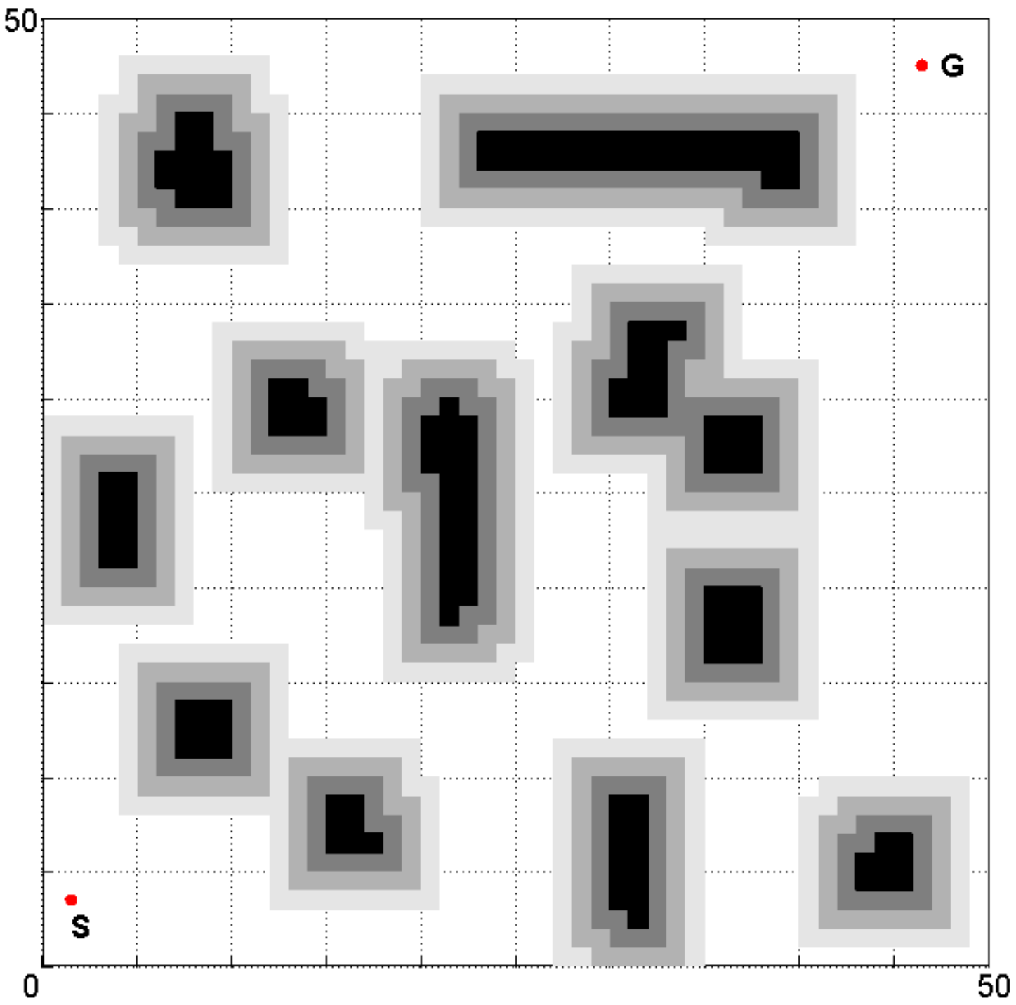
3.1. Improved Environment Model

When the conventional A* algorithm is applied for path planning, the environment is divided into two states: passable regions and forbidden regions. In the path searching process, the states in the forbidden regions would not be traversed and all states in the passable regions are equivalent to each other for the robot. That is to say, no matter how far or close a state is from the obstacles, the robot would spend the same safety cost to pass through the state. However, practically, the safety threat of a robot from the obstacles is inversely proportional to the distance between them. What is more, the expanding obstacles would cover some passable regions and may block the optimal path. For solving this problem, we may introduce the safety cost into the evaluation function of the conventional A* algorithm, but the computation amount is large and the efficiency of the algorithm would be reduced greatly. Therefore, we take the safety threat into account in environment modeling so that the danger coefficient calculation of each state is not required in the path searching process.

In order to avoid excessive amount of calculation, some agreements have been made, as follows:

• The danger coefficient of each state is calculated according to the shortest distance from the state to obstacles. If there is more than one nearest obstacle, only one time computation is needed.
• The danger coefficient of a state is inversely proportional to the minimum distance between the state and obstacles.
• If the minimum distance between a state and obstacles is not less than the given safe distance, the danger coefficient of the state is set to zero.

According to the above rules, the environment model shown in Figure 1 is rebuilt and the danger coefficient of each state is computed and stored in the new improved environment model, as shown in Figure 3.

In Figure 3, the black regions represent the actual obstacles while the grey regions around the obstacles represent the threatened regions. The darker the color of a state is, the greater the danger coefficient is and vice versa. The safe distance between the robot and obstacles is 3 m; if the minimum distance between a state and obstacles is not less than 3 m, the danger coefficient of the state is set to zero.

3.2. Improved Evaluation Function

Evaluation function is the core of A* algorithm. An appropriate evaluation function not only ensures the algorithm to search out the optimal path but also reduces the number of traversal states and improves the efficiency of the algorithm. Nevertheless, in the conventional A* algorithm only the distance cost of the robot has been considered, meaning that the shorter the distance it is, the better the path will be. As a result, the algorithm has only searched the shortest path, which is not necessarily a safe path. In order to obtain a safe path, it is necessary to introduce the safety cost into the evaluation function after the improvement of environment model proposed in Section 3.1. Thus, the actual path cost from state X to S can be expressed as

$$\mathrm{g}\left(X\right)={{\displaystyle \sum }}_{i=1}^n\left({\omega }_1{l}_i+{\omega }_2{s}_i\right),$$

(2)

where, n indicates the number of sections of the path from S to X, ω₁ and ω₂ indicate the weighted coefficients of different parameters, and ω₁ + ω₂ = 1; l_i indicates the length of the i-th section of the path, and s_i indicates the safety cost of the i-th section of the path. Since the i-th section of the path passes through two adjacent states and the safety cost of the path section is not only related to the distance from obstacles but also the length of the path section, we define the safety cost s_i as

$$s_i=d_{i1}{l}_{i1}+d_{i2}{l}_{i2},$$

(3)

where d_i1 and d_i2 respectively indicate the danger coefficients of the two states the path section passes through and l_i1 and l_i2 respectively indicate the lengths of the path section in the two adjacent grids and l_i1 + l_i2 = l_i.

As the robot can move along the diagonal direction in the grid map and the safety cost of the path from X to the goal state G is unable to be computed, the heuristic function h(X) is defined to be proportional to the diagonal distance from X to G. Assuming X’s coordinates are (x₁, y₁) and G’s coordinates are (x_G, y_G) and x = |x₁ − x_G|, y = |y₁ − y_G|, then the diagonal distance l(X) from X to G can be expressed as l(X) = |x − y| + min{x, y} × $\sqrt{2}$. In order to match g(X), the estimated path length should be multiplied by the same weight ω₁, thus

$$h\left(X\right)={\omega }_{1}l\left(X\right)={\omega }_1\left(\left|x-y\right|+\min \left\{x,y\right\}\times \sqrt{2}\right).$$

(4)

According to Equations (1)–(4), the evaluation function f(X) of the improved A* algorithm can be expressed as

$$f\left(X\right)={{\displaystyle \sum }}_{i=1}^n[{\omega }_1{l}_i+{\omega }_2\left(d_{i1}{l}_{i1}+d_{i2}{l}_{i2}\right)]+{\omega }_1\left(\left|x-y\right|+\min \left\{x,y\right\}\times \sqrt{2}\right).$$

(5)

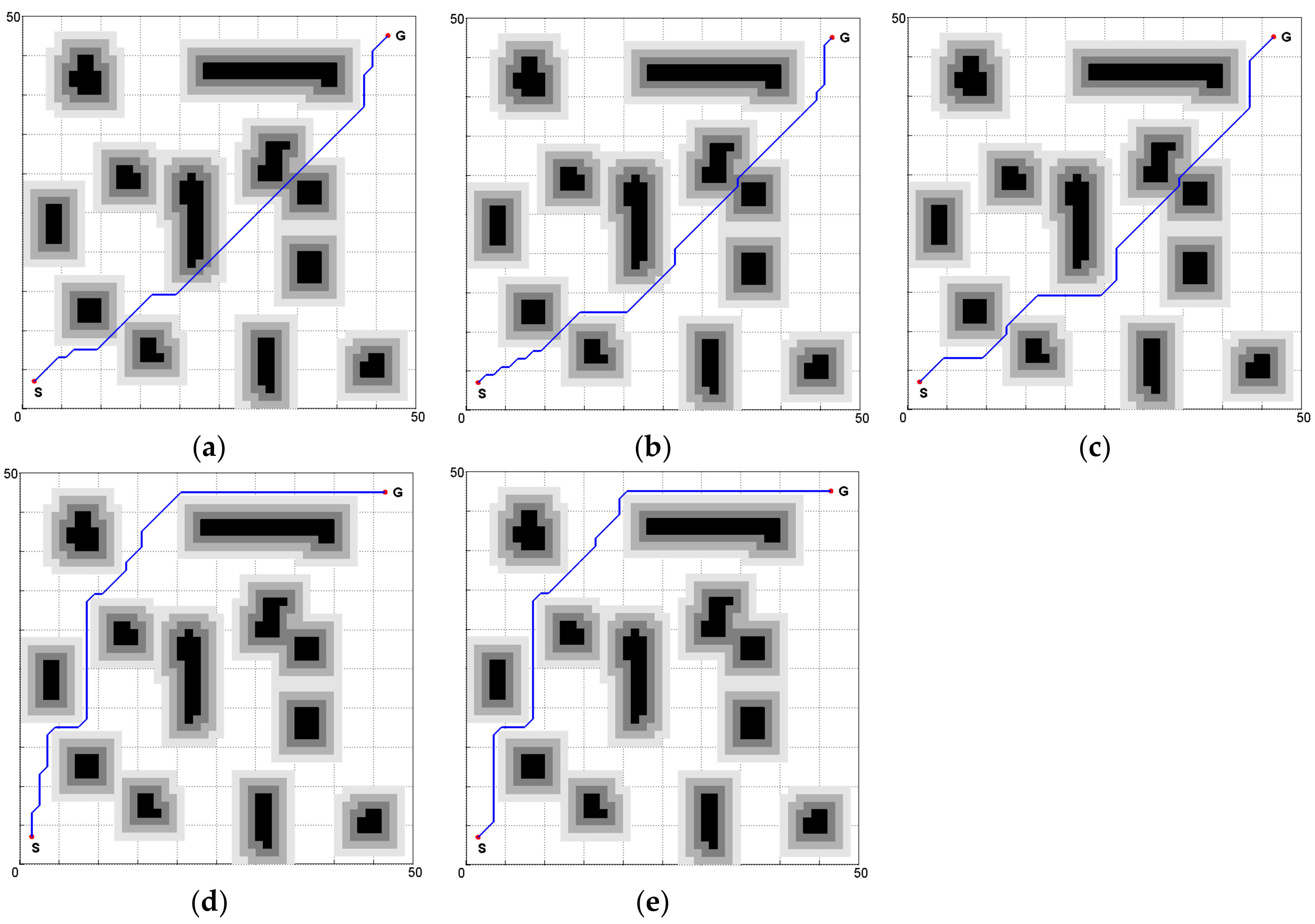
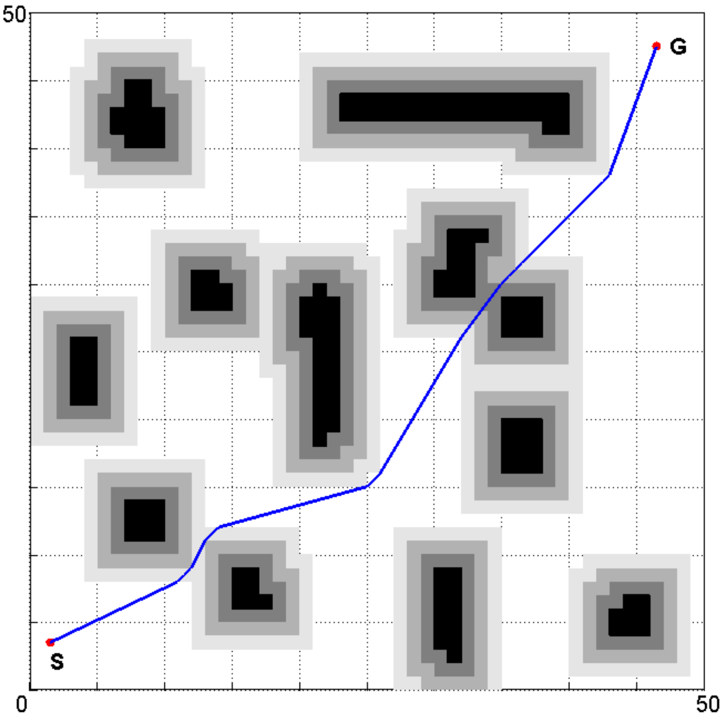
3.3. Algorithm Simulation

The parameter weights ω₁ and ω₂ of the evaluation function are presented and different weights will lead to different results. In order to study the influence of weight coefficients on the path planning, five groups of different weights (ω₁ = 0.9, ω₂ = 0.1; ω₁ = 0.7, ω₂ = 0.3; ω₁ = 0.5, ω₂ = 0.5, ω₁ = 0.3, ω₂ = 0.7, ω₁ = 0.1, ω₂ = 0.9) were chosen to carry out simulations for the improved environment model. The simulation results are shown in Figure 4.

The specific parameters of planning results shown in

Table 1. Path planning of the improved A* algorithm.

ω1:ω2	Path Length (m)	Length of Risky Path	Length of Dangerous Path
0.9:0.1	66.74	22.63	12.73
0.7:0.3	68.50	17.97	6.66
0.5:0.5	70.25	13.31	5.24
0.3:0.7	80.21	0	0
0.1:0.9	80.21	0	0

are where the risky path indicates the path in the threatened regions and the dangerous path indicates the path in the state where the distance from the obstacles is less than half of the safe distance.

It can be seen from Table 1 that the greater the distance weight coefficient ω₁ is, the shorter the length of the planned path. In addition to increasing the safety cost weight coefficient ω₂, the lengths of both the risky path and dangerous path become smaller; this indicates that the planned path becomes safer as the path length becomes longer.

The influence of each weight coefficient on the performance of planned path can be determined from a comparison and is consistent with our expectations. In actual use, the weight coefficients should be set as required. Different results, such as the shortest path or the safest path, can be obtained by setting different weights heuristically. In general, all parameters of the planned path should be taken into account to optimize the planning result. Table 1 demonstrates that the performance of the planned path is excellent when ω₁ = 0.5 and ω₂ = 0.5; the planning result is as shown in Figure 4c. From a comparison of Figure 2 and Figure 4c, we can easily see that the path planned by using the improved A* algorithm is farther away from the path planned obtained by using the conventional A* algorithm. This demonstrates that the improved A* algorithm can determine a safer path.

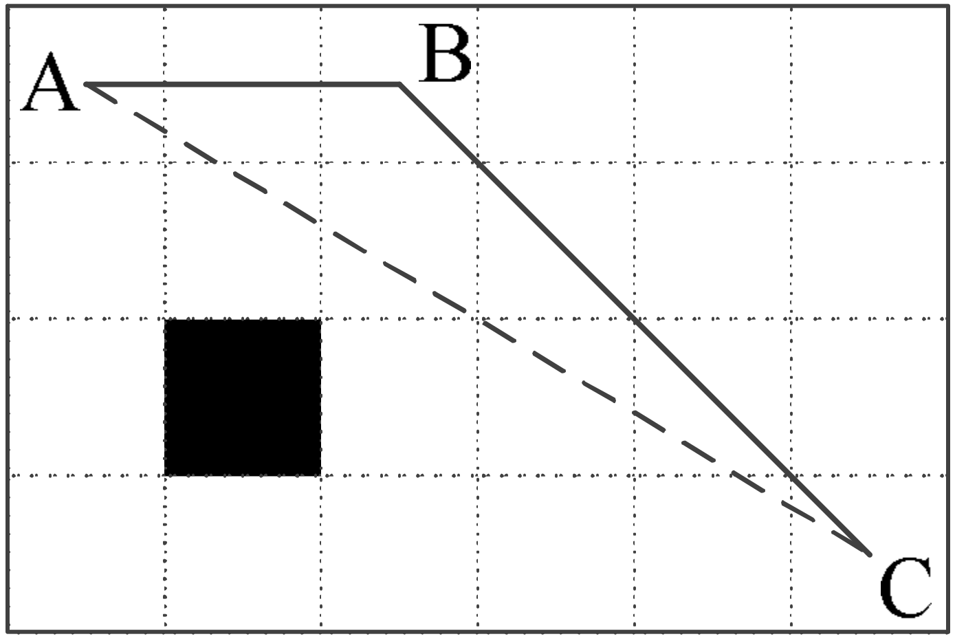
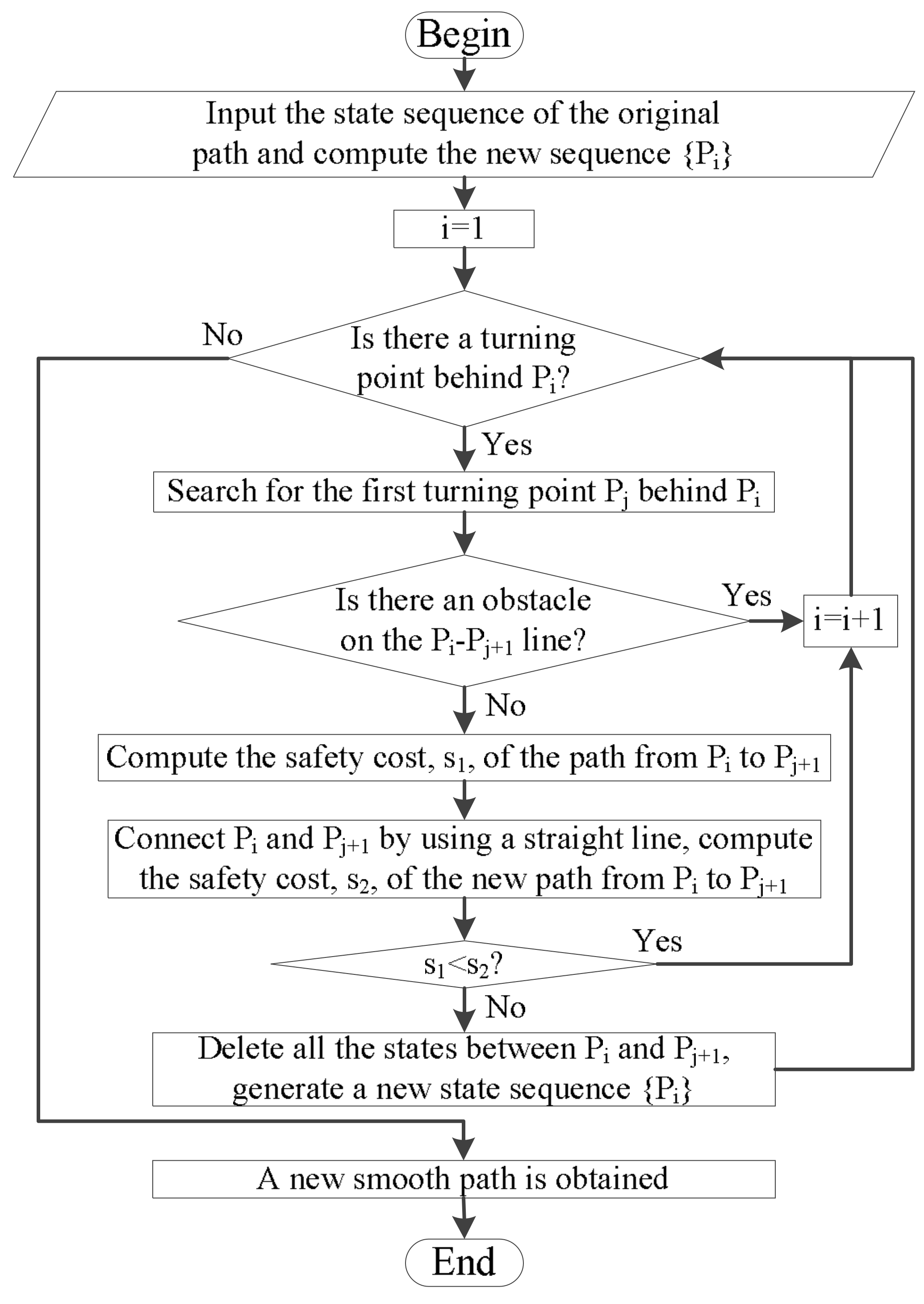
3.4. Path Smoothing Method

From Figure 4c, we can see that a predominant portion of the planned path is within the safe regions; however, there are many turning points on the path which are detrimental to the robot’s movement. Accordingly, it is necessary to smooth the path.

The planning result of A* algorithm is a series of adjacent states. By connecting these adjacent states with straight lines, we can obtain the planned path. To reduce the turning points of the path, we may traverse the path from the initial state to the goal state. For every state X except S and G on the path, we connect the two adjacent states of X by a straight line. If there is no obstacle on the line, then X is deleted and the path is renewed. However, this method does not consider the safety cost of the new path. The number of turning points on the path is reduced but the new path may be closer to obstacles, reducing its safety. As shown in Figure 5, the path AC has fewer turning points than the path ABC, but it is closer to the obstacle.

To keep the new smooth path away from obstacles, a path evaluation mechanism is adopted in the path smoothing process which compute the safety cost of the new path and the old path. The new path can be adopted only when the safety cost is not increased. Concurrently, to improve the flexibility of the path smoothing process, the intersection points between the original path and the map grid lines are added into the state sequence of the original path to generate a new sequence. The flow diagram of the path smoothing method is shown in Figure 6.

The obtained smooth path is shown in Figure 7 which uses the proposed path smoothing method to process the planned path of Figure 4.

Obviously, the smooth path has fewer turning points and smaller turning angles than the path shown in Figure 4. As such, it is more suitable for the robot’s movement. The parameter comparison of the two paths is shown in

Table 2. Path comparison before and after smoothing process.

Path	Path Length (m)	Turning Times (Times)	Sum of Turning Angles (Degree)	Length of Risky Path (m)	Length of Dangerous Path (m)
Before smoothing	70.25	12	540.0	13.31	5.24
After smoothing	66.49	9	168.89	12.89	5.16

.

It can be seen from Table 2 that the smoothing process reduces the path length by 5.4%, reduces the turning times by 25.0%, and reduces the sum of turning angles by 68.7%. At the same time, the length of a risky path is decreased by 3.2% and the length of a dangerous path is decreased by 1.5%. This demonstrates that the path smoothing method is able to smooth the path without decreasing the safety of the path.

3.5. Performance Analysis of the Improved A* algorithm

To analyze the improvement effect, we applied the method proposed in J.D. Hernández et al. [34] to search for the optimal path in the same environment. Risk zones around the vehicle were established to keep the path away from obstacles. The vehicle was assumed to be point-size and occupied only one state at a time. The risk zones around the vehicle consisted of three zones, as shown in Figure 8a. The function of the risk zones is presented as follows.

$$Risk\left(q\right)=\{\begin{array}{cc}1.6,& \hfill if Collision\left({zone}_1\right)\\ 1.4,& \hfill if Collision\left({zone}_2\right)\\ 1.2,& \hfill if Collision\left({zone}_3\right)\\ 1,& \hfill if not Collision(any zone)\end{array}\hspace{1em}q={\left[x,y,\psi \right]}^T$$

(6)

For the RRT* algorithm (Please find additional detail in S. Karaman et al. [10]), the radius of the set Xnear of vertices is eight, the parameter η of the function Steer is set to two, and the number of iterations is set to 1000. Because of the random nature of the sampling process, the improved RRT* algorithm planned different paths each time. Large amounts of simulation were executed and the optimal path we obtained is shown in Figure 8b.

Figure 2, Figure 7, and Figure 8b show the paths generated by using the conventional A* algorithm, the improved A* algorithm, and the improved RRT* algorithm, respectively. The performance comparisons of the three algorithms are shown in

Table 3. Performance comparisons of the conventional A*, improved RRT*, and improved A*.

Parameter	Conventional A*	Improved RRT*	Improved A*
Path length (m)	66.15	65.72	66.49
Turning times (times)	14	11	9
Sum of turning angles (degree)	630.00	124.36	168.89
Length of risky path (m)	41.53	19.25	12.89
Length of dangerous path (m)	30.83	8.45	5.16
Computation time (s)	0.06	17.84	0.24

.

Table 3 shows us the comparisons of the conventional A* algorithm, the improved RRT* algorithm and the improved A* algorithm. Compared to the conversional A* algorithm, although the improved A* algorithm increased the path length by 0.5% and computation time by a factor of three, it reduced the turning time and sum of turning angles by 35.7% and 73.2%, respectively. It also reduced the length of the risky and dangerous paths by 69.0% and 83.3%, respectively. Compared to the improved RRT* algorithm, the improved A* algorithm increased the path length and the sum of turning angles by 1.2% and 35.8%, respectively; however, it reduced the turning time by 18.2% and also reduced the length of the risky and dangerous path by 33.0% and 38.9%, respectively. In these simulations, the improved RRT* algorithm produced the shortest path; however, as it needed to check for collision for each sampled configuration and the intermediate steps when connecting to others, the computation time of the improved RRT* algorithm was two orders of magnitude larger than that of the other two algorithms.

The comparison result shows that, compared to the conventional A* algorithm and the improved RRT* algorithm, the improved A* algorithm can determine a better path for the actual movement of the robot. It also proves the feasibility and effectiveness of the improved A* algorithm.

4. Path Planning in Complex Terrains

The improved A* algorithm proposed in Section 3 was adopted for mobile robot path planning in a single terrain environment and has achieved remarkable results. However, in a complex terrain environment, the movement speeds of the robot in different terrains were not equal. In this case, the shorter path length did not result in a shorter movement time. Accordingly, it was necessary to improve the evaluation function and evaluate the planned path by the movement time of the robot. In addition, in the improved environment model proposed in Section 3.1, the danger coefficient of each state was related to the minimum distance between the state and obstacles. However, in a complex terrain environment, the danger coefficient of each state was also related to its terrain, so we needed to improve the environment model to enhance its applicability. This section will elaborate on the path planning process in a complex terrain environment and verify the planning results by simulation experiments.

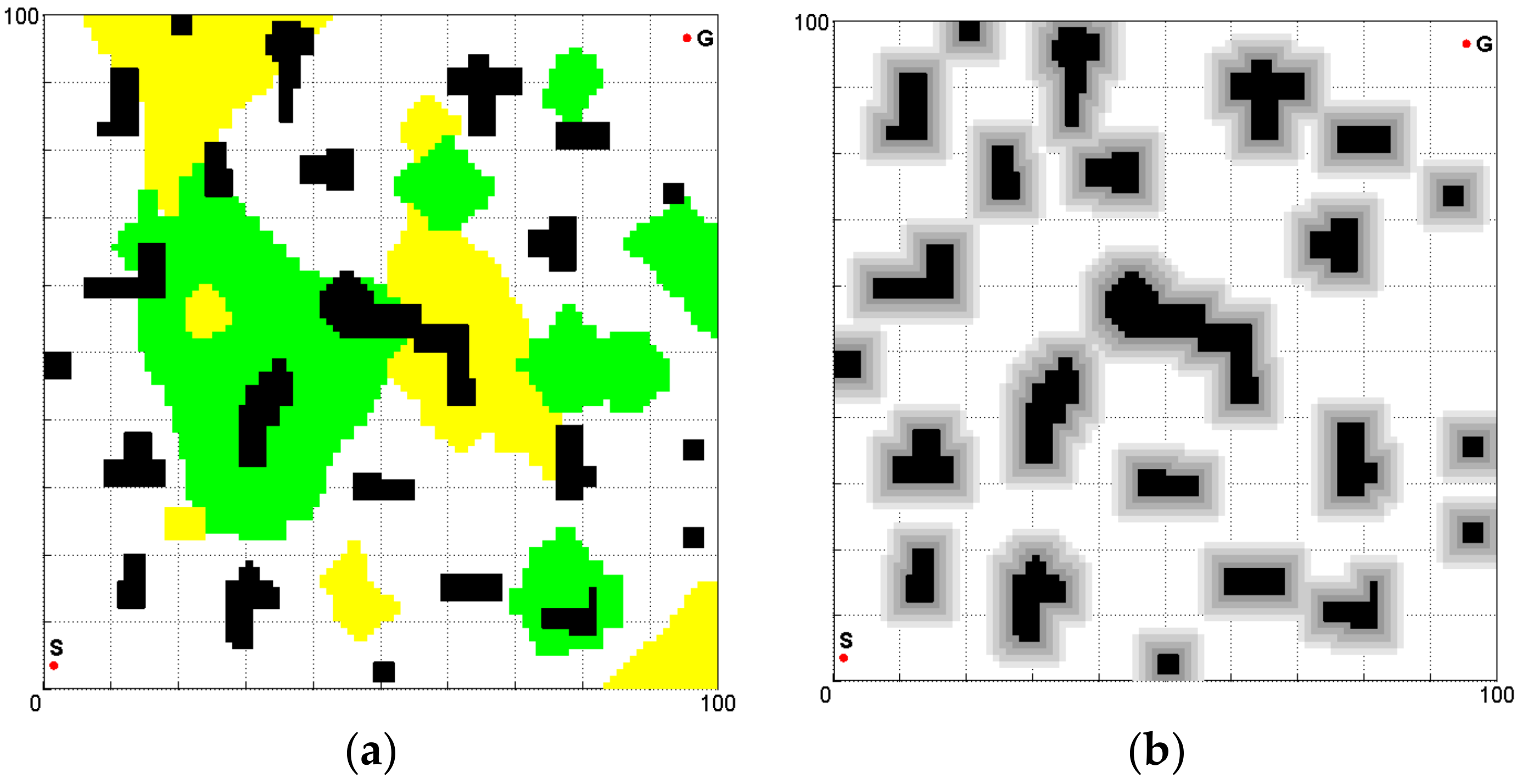
4.1. Complex Terrain Environment Model

Common terrains in the wild include flat land, grassland, mountain land, marsh land, rivers, lakes, etc. If we set the marsh land, rivers, lakes, and other impassable areas as obstacle areas and distinguish the flat land, grassland, and mountain land with different colors, then a complex terrain environment model can be established, as shown in Figure 9.

Figure 9 represents the square with a side length of 100 m, divided into 100 × 100 grids. Figure 9a indicates the terrain model. The obstacles and three different kinds of terrains are distributed irregularly in the regions, wherein the black regions represent obstacles, the yellow regions represent mountain land regions, the green areas represent grassland regions, and the other areas represent flat land regions. Figure 9b indicates the obstacle model. S’s position coordinates are (2, 4) and G’s (96, 97).

4.2. Evaluation Function

In a single terrain environment, the robot moves at a constant speed. A shorter path length means a reduced movement time of the robot. But in complex terrain environment, we need to take the shortest movement time as the goal of path planning under the premise of ensuring the safety of the robot. Moreover, the improved evaluation function proposed in Section 3.2 has two parameters: distance cost and safety cost. The physical meanings and units of the two parameters are different so the evaluation function, which is the weighted sum of the two parameters, lacks physical meaning and is hard to understand. Therefore, the two parameters are converted into time cost so that the units can be unified and their physical meanings are clear as well.

The distance of the path is related to the speed and movement time of the robot; the distance cost of the path can be expressed as a function of speed and time cost. The safety cost of the path is inversely proportional to the distance between the path and obstacles. If a robot is moving along the path, when it nears obstacles it needs to slow down to ensure safety. Accordingly, the safety threat from obstacles affects the speed and movement time of the robot; namely, the safety cost can be converted into time cost. Thus, the actual path cost from X to S can be expressed as

$$\mathrm{g}\left(X\right)={{\displaystyle \sum }}_{i=1}^n(\frac{l_{i1}}{v_{i1}\left(1-p_{i1}\right)}+\frac{l_{i2}}{v_{i2}\left(1-p_{i2}\right)}),$$

(7)

where, v_i1 and v_i2 respectively indicate the speeds of the robot moving at the two states where the path section locates. The speeds are only relative to the terrains that the states are in; p_i1 and p_i2 indicate the speed reduction ratios of the robot affected by the safety cost when moving on the i-th section of the path. When the minimum distance between a state and obstacles exceeds the safe distance, the speed reduction ratio of the state is set to zero.

The heuristic function can be expressed as

$$h\left(X\right)=\frac{l\left(X\right)}{v}=\frac{\left|x-y\right|+\min \left\{x,y\right\}\times \sqrt{2}}{v},$$

(8)

where v indicates the speed of the robot moving on flat land. According to Equations (1), (7), and (8), the evaluation function of the improved A* algorithm can be expressed as

$$f\left(X\right)={{\displaystyle \sum }}_{i=1}^n(\frac{l_{i1}}{v_{i1}(1-p_{i1})}+\frac{l_{i2}}{v_{i2}\left(1-p_{i2}\right)})+\frac{\left|x-y\right|+\min \left\{x,y\right\}\times \sqrt{2}}{v}.$$

(9)

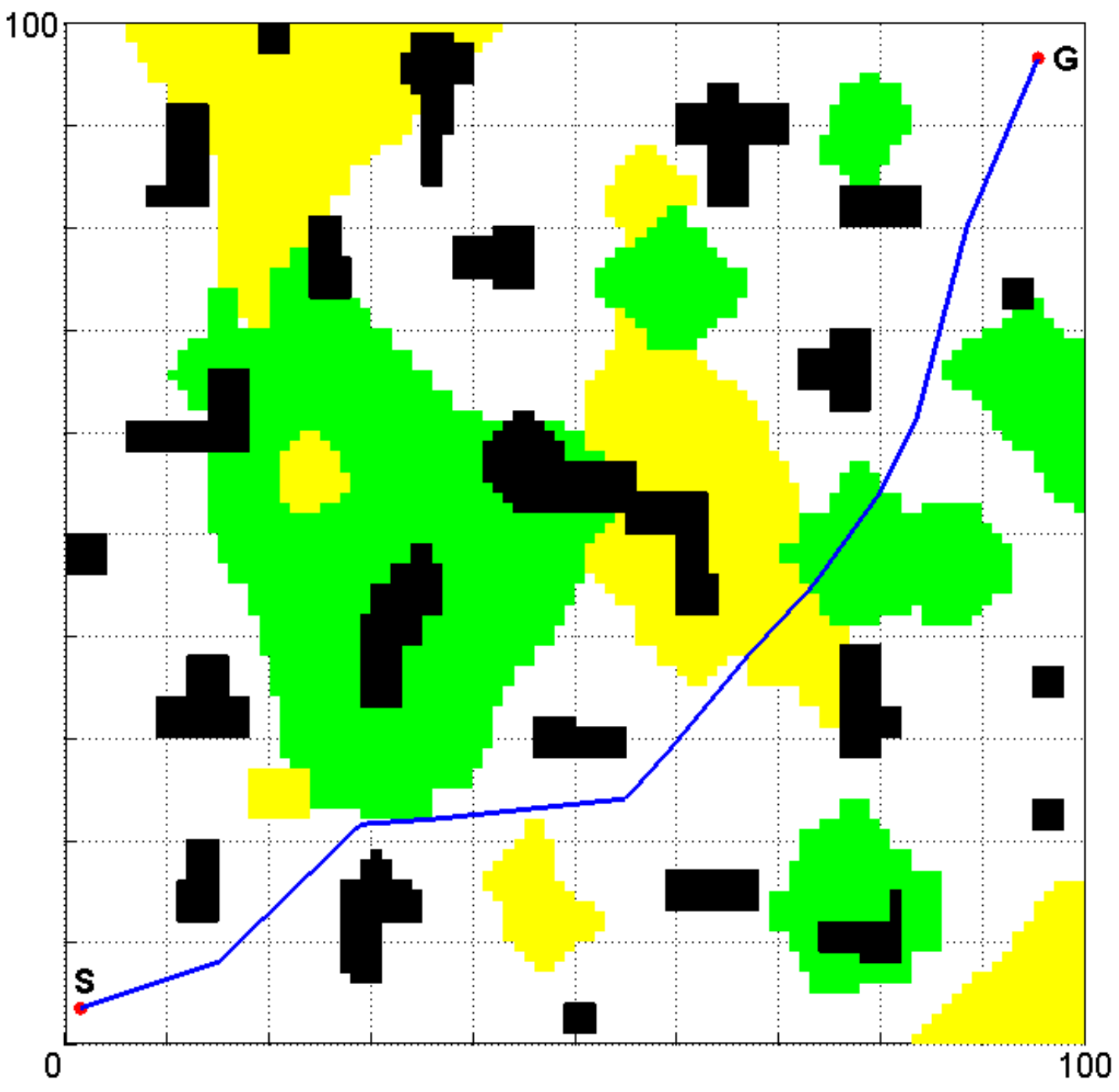
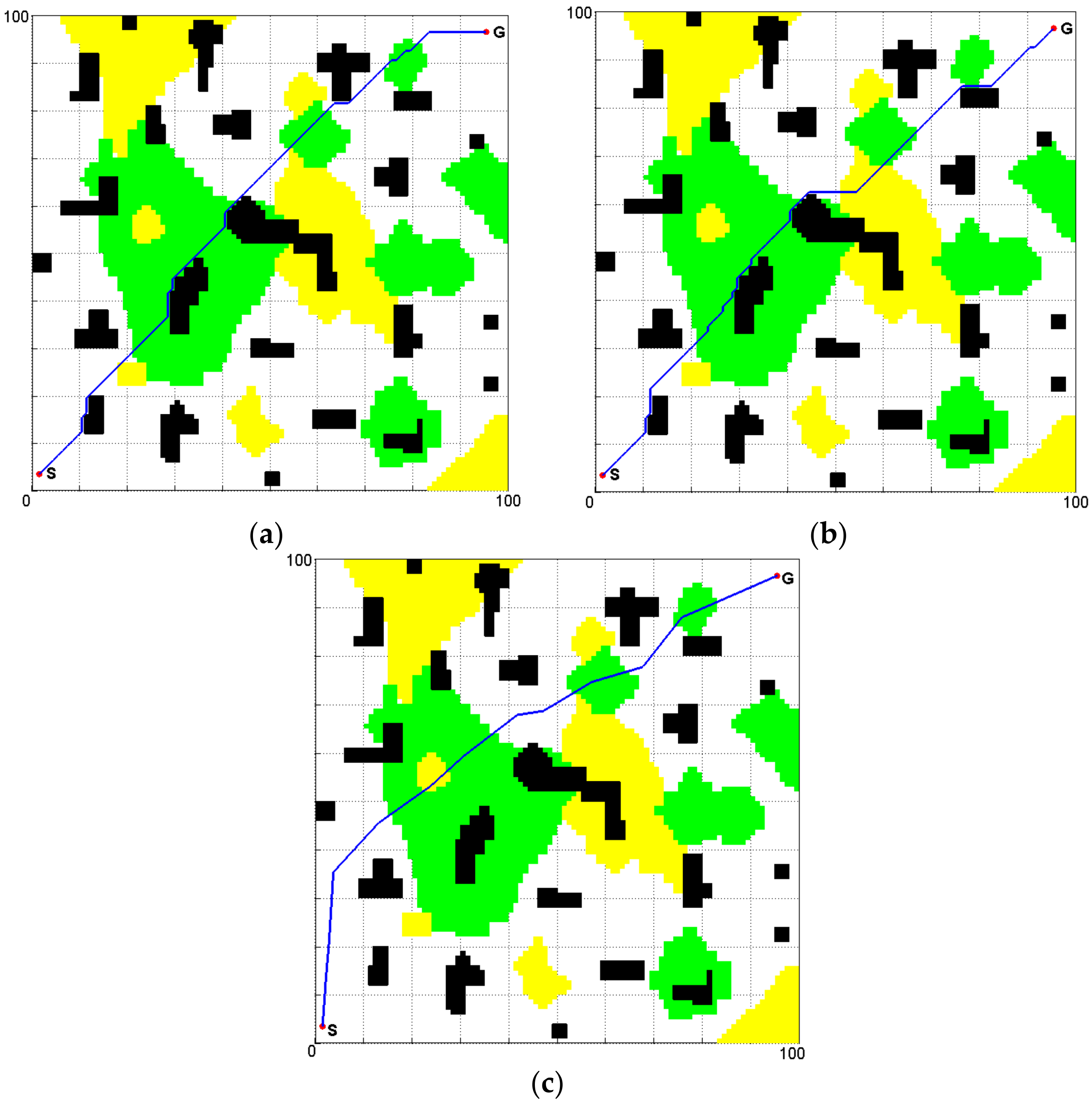
4.3. Simulation Experiments and Analysis in Complex Terrain Environment

Assume the average speeds of the robot moving on flat land, grassland, and mountain land are 2 m/s, 1.6 m/s, and 1.2 m/s, respectively. The speed of the robot should be adjusted according to the minimum distance between the robot and obstacles; the adjustment rules are shown in

Table 4. The adjustment rules of the robot speed.

Minimum Distance (m)	Speed Reduction Ratio
0~1	50%
1~2	40%
2~3	30%
3~4	20%
4~5	10%
>5	0%

.

The smooth path generated by simulation is shown in Figure 10.

It can be seen from Figure 10 that the planned path keeps a certain distance from the obstacles to ensure the safety of the path. A predominant portion of the path is on flat land because the robot moves faster on it. Nevertheless, there is also a part of path which passes through mountain land and grassland instead of detouring around them to favor a path exclusively on flat land. This is because the detouring process would take more time.

The ant colony optimization (ACO) algorithm, the conventional A* algorithm, and the improved RRT* algorithm are applied to search the shortest paths respectively in the same environment. The parameters configuration of the ACO is shown in

Table 5. Parameters configuration of the ant colony optimization algorithm.

K	M	α	β	ρ	Q
15	18	1	4	0.35	140

, where K indicates the largest number of iterations, M indicates the total number of ants, α and β indicate the stimulating factors of pheromone concentration and visibility respectively, ρ indicates the coefficient of the pheromone volatilization, and Q indicates the initial value of the pheromone concentration. For the RRT* algorithm, the risk zones around the vehicle consisted of four zones and the function of the risk zones is presented as follows.

$$Risk\left(q\right)=\{\begin{array}{cc}1.8,& \hfill if Collision\left({zone}_1\right)\\ 1.6,& \hfill if Collision\left({zone}_2\right)\\ 1.4,& \hfill if Collision\left({zone}_3\right)\\ 1.2,& \hfill if Collision\left({zone}_4\right)\\ 1,& \hfill if not Collision(any zone)\end{array}\hspace{1em}q={\left[x,y,\psi \right]}^T$$

(10)

The radius of the set Xnear of vertices is 15, η = 2, the number of iterations was set to 1500. The planning results of the three algorithms are shown in Figure 11.

Obviously, the planned paths generated by the ACO algorithm and the conventional A* algorithm had many turning points and also directly passed through a large area of grassland and mountain land. Both paths were close to the obstacles and were not time-optimal paths. The paths generated by the improved RRT* algorithm and the improved A* algorithm kept away from the obstacles.

Table 6. Performance comparison of the four algorithms in complex terrain environment.

Parameter	ACO	Conventional A*	Improved RRT*	Improved A*
Path length (m)	141.89	141.89	144.72	144.29
Turning times (times)	17	22	11	10
Sum of turning angles (degree)	765.00	990.00	193.84	150.92
Length of risky path (m)	86.88	85.78	14.71	28.25
Length of dangerous path (m)	57.18	56.32	0.49	2.10
Computation time (s)	2.18	0.16	47.39	0.64
Movement time (s)	127.23	127.54	81.30	79.56

shows the detailed parameters of the four paths shown in Figure 10 and Figure 11.

Although the improved A* algorithm increased the path length by 1.7%, Table 6 demonstrates that it reduced the turning times by 41.2%, reduced the sum of turning angles by 80.3%, reduced the length of risky path and dangerous path by 67.5% and 96.3% respectively, reduced the computation time by 70.6%, and it eventually led to a 37.5% fall in the movement time of the robot compared to the ACO algorithm. Compared to the conventional A*algorithm, the improved A* algorithm increased the path length by 1.7% and increased the computation time by a factor of three, but it reduced the turning times by 54.5%, reduced the sum of turning angles by 84.8%, reduced the length of risky path and dangerous path by 67.1% and 96.3% respectively, and it eventually led to a 37.6% decrease in the movement time of the robot. Compared to the improved RRT* algorithm, the improved A* algorithm increased the length risky path and dangerous path by 92.0% and 3.3 times respectively; however, it reduced the path length by 0.3%, reduced the turning times by 9.1%, reduced the sum of turning angles by 22.1%, reduced the movement time by 2.1%, and, more importantly, the computation time dropped by two orders of magnitude.

The comparison results show that the planned path of the improved A* algorithm was more suitable for the actual movement of the robot; it proves the feasibility and effectiveness of the improved A* algorithm for solving safe path planning problems in complex terrain environment.

5. Conclusions and Suggestions

This paper studies the path planning problem of mobile robot based on an improved A* algorithm in a two-dimensional complex terrain environment. The conclusions and suggestions are as follows:

• In light of the disadvantages of the conventional A* algorithm, an improved A* algorithm is presented in this paper for the path planning of mobile robot. A new environment modeling method is proposed in which the evaluation function of A* algorithm is improved by taking into account of the safety cost. Accordingly, the planned path can be farther away from obstacles to ensure the safety of the path. A new path smoothing method is also proposed which introduces a path evaluation mechanism into the smoothing process; this is applied to smooth the path without safety reduction. Compared to the conventional A* algorithm, although the improved A* algorithm increased the path length by 0.5% and computation time by a factor of three, it reduced the turning times and sum of turning angles by 35.7% and 73.2%, respectively. It also reduced the length of risky and dangerous paths by 69.0% and 83.3%, respectively. Compared to the improved RRT* algorithm, the improved A* algorithm increased the path length and the sum of turning angles by 1.2% and 35.8%, respectively; however, it reduced the turning times by 18.2%, and also reduced the length of risky and dangerous paths by 33.0% and 38.9%, respectively. The computation time of the improved RRT* algorithm was two orders of magnitude larger than that of the improved A* algorithm.
• In order to solve the path planning problems in complex terrains, a complex terrain environment model, which considered flat land, grassland, mountain land, and obstacles, is established in this paper. The distance and safety cost of the evaluation function of the A* algorithm were converted into time cost so that the units could be unified and their physical meanings clarified. Compared to the ACO algorithm, although the path length was increased by 1.7%, the improved A* algorithm reduced the turning times by 41.2%, reduced the sum of turning angles by 80.3%, reduced the length of risky and dangerous paths by 67.5% and 96.3% respectively, reduced the computation time by 70.6%, and it eventually led to a 37.5% fall in the movement time of the robot. Compared to the conventional A* algorithm, the improved A* algorithm increased the path length by 1.7% and increased the computation time by a factor of three; however, it reduced the turning times by 54.5%, reduced the sum of turning angles by 84.8%, reduced the length of risky and dangerous paths by 67.1% and 96.3% respectively, and it eventually led to a 37.6% fall in the movement time of the robot. Compared to the improved RRT* algorithm, the improved A* algorithm increased the length of risky and dangerous paths by 92.0% and 3.3 times respectively; however, it reduced the path length by 0.3%, reduced the turning times by 9.1%, reduced the sum of turning angles by 22.1%, reduced the movement time by 2.1%, and more importantly, the computation time dropped in two orders of magnitude.
• Compared to the conventional A* algorithm, the improved A* algorithm achieved remarkable results and was more suitable for the path planning of mobile robots. However, the path searching time was considerably increased, especially for the path planning of complex terrain environment whose consuming time was increased by a factor of three. Through analysis, we can know that it is because of the substantial increase in the number of traversal states of the improved A* algorithm. Therefore, it is suggested that the future work should be focused on improving the computational efficiency of the improved A* algorithm so as to enhance its real-time performance.
• In our recent studies, we assume that the environment is completely known. Accordingly, path planning research in unknown environments may be the next step of our research.

References

1. Choset, H.; Lynch, K.M.; Hutchinson, S.; Kantor, G.A.; Burgard, W.; Kavraki, L.E.; Thrun, S. Principles of Robot Motion: Theory, Algorithms, and Implementations; MIT Press: Cambridge, MA, USA, 2005; pp. 1–15. [Google Scholar]
2. LaValle, S.M. Planing Algorithms; Cambridge University Press: Cambridge, UK, 2006; pp. 1–26. [Google Scholar]
3. Wei, W.; Ouyang, D.T.; Lu, S.; Feng, Y.X. Multiobjective path planning under dynamic uncertain environment. Chin. J. Comput. 2011, 34, 836–846. [Google Scholar] [CrossRef]
4. Wang, F.; Wan, L.; Xu, Y.R.; Zhang, Y.K. Path planning based on improved artificial potential field for autonomous underwater vehicles. J. Huazhong Univ. Sci. Technol. 2011, 39, 184–187. [Google Scholar]
5. Gu, Q.; Dou, F.Q.; Ma, F. Energy optimal path planning of electric vehicle based on improved A* algorithm. Trans. Chin. Soc. Agric. Mach. 2015, 46, 316–322. [Google Scholar]
6. Zhu, D.Q.; Yan, M.Z. Survey on technology of mobile robot path planning. Control Decis. 2010, 25, 961–967. [Google Scholar]
7. Kavraki, L.E.; Svestka, P.; Latombe, J.C.; Overmars, M.H. Probabilistic roadmaps for path planning in high-dimensional configuration spaces. IEEE Trans. Robot. Autom. 1996, 12, 566–580. [Google Scholar] [CrossRef]
8. Lavalle, S.M. Rapidly-exploring random trees: A new tool for path planning. In Algorithmic and Computational Robotics New Directions; Taylor & Francis: Oxford, UK, 1998; pp. 293–308. [Google Scholar]
9. Hsu, D. Randomized Single-Query Motion Planning in Expansive Spaces. Ph.D. Thesis, Stanford University, Stanford, CA, USA, 2000. [Google Scholar]
10. Karaman, S.; Frazzoli, E. Incremental sampling-based algorithms for optimal motion planning. In Proceedings of the Robotics: Science and Systems Conference, Zaragoza, Spain, 27–30 June 2010; pp. 5326–5332. [Google Scholar]
11. Yu, Z.Z.; Yan, J.H.; Zhao, J.; Chen, Z.F.; Zhu, Y.H. Mobile robot path planning based on improved artificial potential field method. J. Harbin Inst. Technol. 2011, 43, 50–55. [Google Scholar]
12. Li, G.H.; Tong, S.G.; Cong, F.Y.; Yamashita, A.; Asama, H. Improved artificial potential field-based simultaneous forward search method for robot path planning in complex environment. In Proceedings of the IEEE/SICE International Symposium on System Integration, Nagoya, Japan, 11–13 December 2015; pp. 760–765. [Google Scholar]
13. Thaker, N.; Nikolakopoulos, G.; Gustafsson, T. On-line path planning for an articulated vehicle based on model predictive control. In Proceedings of the IEEE International Conference on Control Applications, Hyderabad, India, 28–30 August 2013; pp. 772–777. [Google Scholar]
14. Chen, W.D.; Zhu, Q.G. Mobile robot path planning based on fuzzy algorithm. Acta Electron. Sin. 2011, 39, 971–974, 980. [Google Scholar]
15. Mobadersany, P.; Khanmohammadi, S.; Ghaemi, S. A fuzzy multi-stage path-planning method for a robot in a dynamic environment with unknown moving obstacles. Robotica 2015, 33, 1869–1885. [Google Scholar] [CrossRef]
16. Wang, K.; Shi, W.R. Back propagation neural network to the application of cleaning robot’s path planning. J. Chongqing Univ. 2009, 32, 349–352. [Google Scholar]
17. Shorakaei, H.; Vahdani, M.; Imani, B.; Gholami, A. Optimal cooperative path planning of unmanned aerial vehicles by a parallel genetic algorithm. Robotica 2016, 34, 823–836. [Google Scholar] [CrossRef]
18. Shi, E.X.; Chen, M.M.; Li, J.; Huang, Y.M. Research on method of global path-planning for mobile robot based on ant-colony algorithm. Trans. Chin. Soc. Agric. Mach. 2014, 45, 53–57. [Google Scholar]
19. Zeng, M.R.; Xi, L.; Xiao, A.M. The free step length ant colony algorithm in mobile robot path planning. Adv. Robot. 2016, 30, 1509–1514. [Google Scholar] [CrossRef]
20. Ziadi, S.; Njah, M.; Chtourou, M. PSO optimization of mobile robot trajectories in unknown environments. In Proceedings of the 13th International Multi-Conference on System, Signals & Devices, Leipzig, Germany, 21–24 March 2016; pp. 774–782. [Google Scholar]
21. Mohanty, P.K.; Parhi, D.R. Optimal path planning for a mobile robot using cuckoo search algorithm. J. Exp. Theor. Artif. Intell. 2016, 28, 35–52. [Google Scholar] [CrossRef]
22. Wang, W.F.; Xu, C.; Yin, B.B.; Du, Z.J. Path planning in dynamic environment based on improved shuffled frog leaping algorithm. J. Jilin Univ. 2016, 54, 857–861. [Google Scholar]
23. Shi, H.; Cao, W.; Zhu, S.L.; Zhu, B.S. Application of an improved A* algorithm in shortest route planning. Geomat. Spat. Inf. Technol. 2009, 32, 208–211. [Google Scholar]
24. Lu, Z.Y.; Cai, T.J. Gravity aided navigation path plan research based on A* algorithm. J. Chin. Inert. Technol. 2010, 18, 556–560. [Google Scholar]
25. Zhan, W.W.; Wang, W.; Chen, N.C.; Wang, C. Path planning strategies for UAV based on improved A* algorithm. Geomat. Inf. Sci. Wuhan Univ. 2015, 40, 315–320. [Google Scholar]
26. Szczerba, R.J.; Galkowski, P.; Glickstein, I.S.; Ternullo, N. Robust algorithm for real-time route planning. IEEE Trans. Aerosp. Electron. Syst. 2000, 36, 869–878. [Google Scholar] [CrossRef]
27. Zhang, Y.N.; Gao, J.Y. Three-dimensional route planning based on an advanced A* algorithm. Flight Dyn. 2008, 26, 48–51. [Google Scholar]
28. Xin, Y.; Liang, H.W.; Du, M.B.; Mei, T.; Wang, Z.L.; Jiang, R.H. An improved A* algorithm for searching infinite neighbourhoods. Robot 2014, 36, 627–633. [Google Scholar]
29. Wang, H.W.; Ma, Y.; Xie, Y.; Guo, M. Mobile robot optimal path planning based on smoothing A* algorithm. J. Tongji Univ. 2010, 38, 1647–1650. [Google Scholar]
30. Shan, W.; Meng, Z.D. Smooth path design for mobile service robots based on improved A* algorithm. J. Southeast Univ. 2010, 40, 155–161. [Google Scholar]
31. Wang, D.J. Indoor mobile-robot path planning based on an improved A* algorithm. J. Tsinghua Univ. 2012, 52, 1085–1089. [Google Scholar]
32. Harabor, D.; Grastien, A. Online graph pruning for pathfinding on grid maps. In Proceedings of the AAAI Conference on Artificial Intelligence, San Francisco, CA, USA, 7–11 August 2011; pp. 1114–1119. [Google Scholar]
33. Cheng, L.P.; Liu, C.X.; Yan, B. Improved hierarchical A-star algorithm for optimal parking path planning of the large parking lot. In Proceedings of the IEEE International Conference on Information & Automation, Hailar, China, 26–31 July 2014; pp. 695–698. [Google Scholar]
34. Hernández, J.D.; Moll, M.; Vidal, E.; Carreras, M.; Kavraki, L.E. Planning feasible and safe paths online for autonomous underwater vehicles in unknown environments. In Proceedings of the 2016 IEEE/RSJ International Conference on Intelligent Robots and Systems, Daejeon, Korea, 9–14 October 2016. [Google Scholar]
35. Dijkstra, E.W. A note on two problems in connexion with graphs. Numer. Math. 1959, 1, 269–271. [Google Scholar] [CrossRef]
36. Moore, E.F. The shortest path through a maze. In Proceedings of the International Symposium on the Theory of Switching, Cambridge, MA, USA, 2–5 April 1957; Harvard University Press: Cambridge, MA, USA, 1959; pp. 285–292. [Google Scholar]
Figure 1. Environment model.
Algorithms 11 00044 g001
Figure 2. Simulation result of A* algorithm.
Algorithms 11 00044 g002
Figure 3. Improved environment model.
Algorithms 11 00044 g003
Figure 4. Planned path of the improved A* algorithm: (a) ω1 = 0.9, ω2 = 0.1; (b) ω1 = 0.7, ω2 = 0.3; (c) ω1 = 0.5, ω2 = 0.5; (d) ω1 = 0.3, ω2 = 0.7; (e) ω1 = 0.1, ω2 = 0.9.
Algorithms 11 00044 g004
Figure 5. Diagram of path smoothing.
Algorithms 11 00044 g005
Figure 6. Flow diagram of the path smoothing method.
Algorithms 11 00044 g006
Figure 7. Smooth path of the improved A* algorithm.
Algorithms 11 00044 g007
Figure 8. Planned path of the improved RRT* algorithm: (a) Risk zones; (b) Planned path.
Algorithms 11 00044 g008
Figure 9. Complex terrain environment model: (a) Terrain model; (b) Obstacle model.
Algorithms 11 00044 g009
Figure 10. Path planning in complex terrain environment by using the improved A* algorithm.
Algorithms 11 00044 g010
Figure 11. Path planning in complex terrain environment by using different algorithms: (a) Simulation result of the ant colony optimization (ACO) algorithm; (b) Simulation result of the conventional A* algorithm; (c) Simulation result of the improved RRT* algorithm.
Algorithms 11 00044 g011