Local Coupled Extreme Learning Machine Based on Particle Swarm Optimization


Abstract
1. Introduction
2. Theoretical Background
2.1. Local Coupled Extreme Learning Machine
| Algorithm 1. The algorithm flow of LC-LEM |
| (1) Input weights , hidden bias and the node address are allocated randomly. |
| (2) The output matrix of the hidden layer is computed using Equation (4). |
| (3) Calculate the output weights between the hidden layer and the output layer based on Equation (5): . |
2.2. Particle Swarm Optimization
3. Local Coupled Extreme Learning Machine Based on the PSO Algorithm
| Algorithm 2. The algorithm flow of LC-PSO-ELM |
(1) Initiate the population (particle).
|
| (2) Iter = 1 |
| (3) While Iter |
| (4) (1) Evaluate the fitness function of each particle (the root means standard error for regression problems and the classification accuracy for classification problems). (2) Modify the position of the particle according to Equations (4)–(8). (3) Iter = Iter +1 |
| (5) end while (6) The optimal parameters of the LC-ELM can be determined. Then, based on the optimized parameters:
|
4. Simulations and Performance Verification
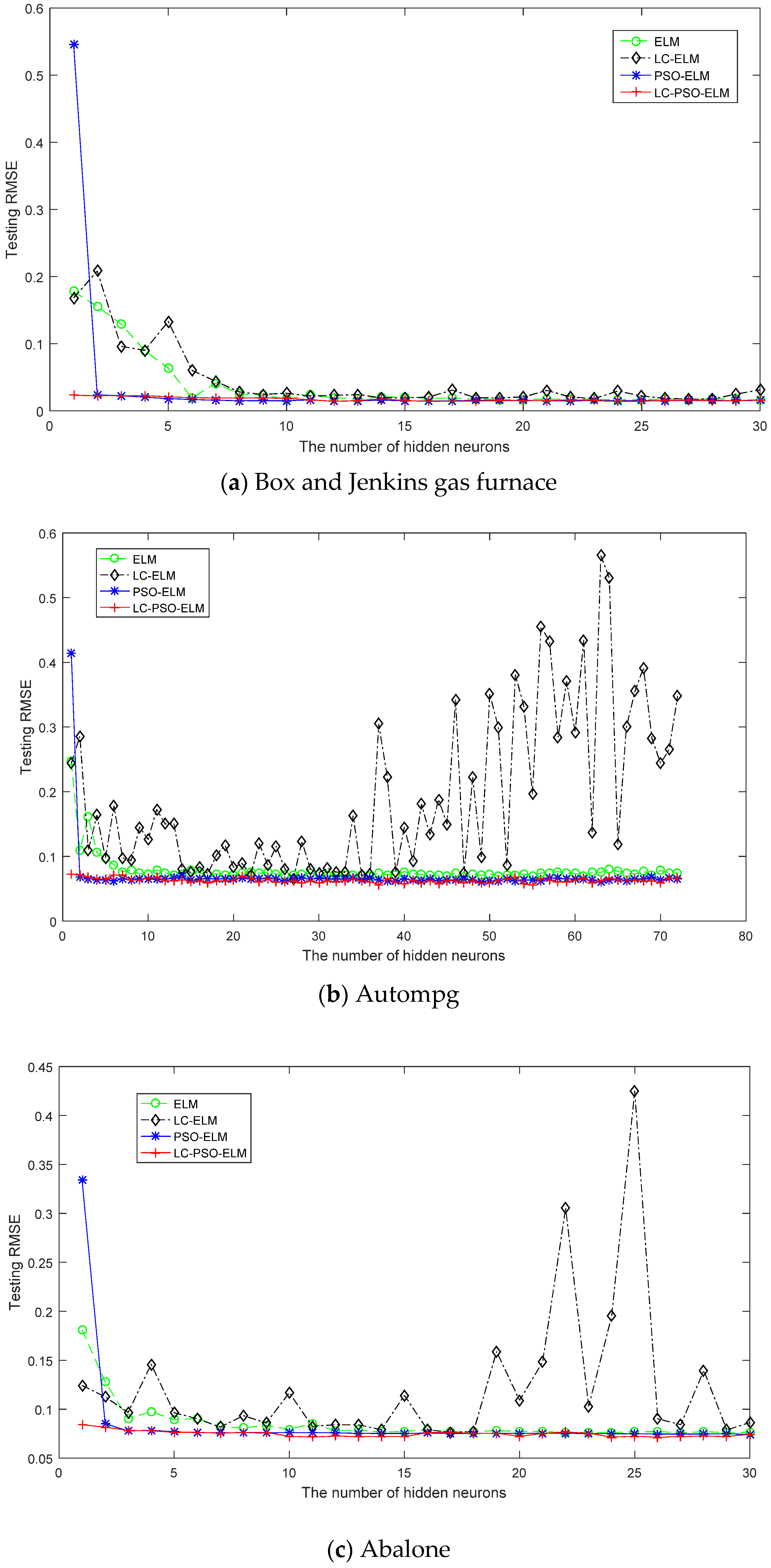
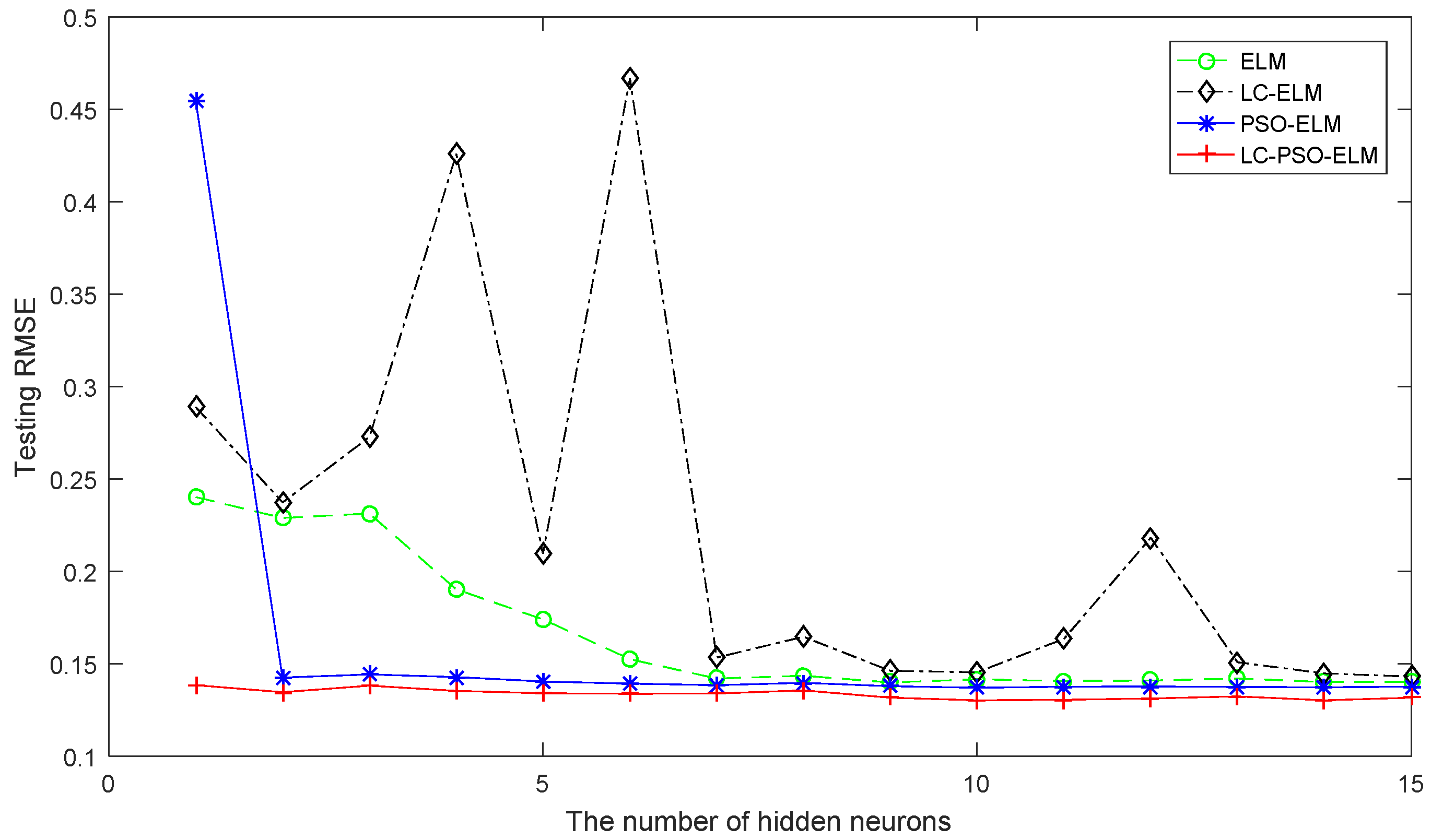
4.1. Performance Comparison of Regression Benchmark Problems
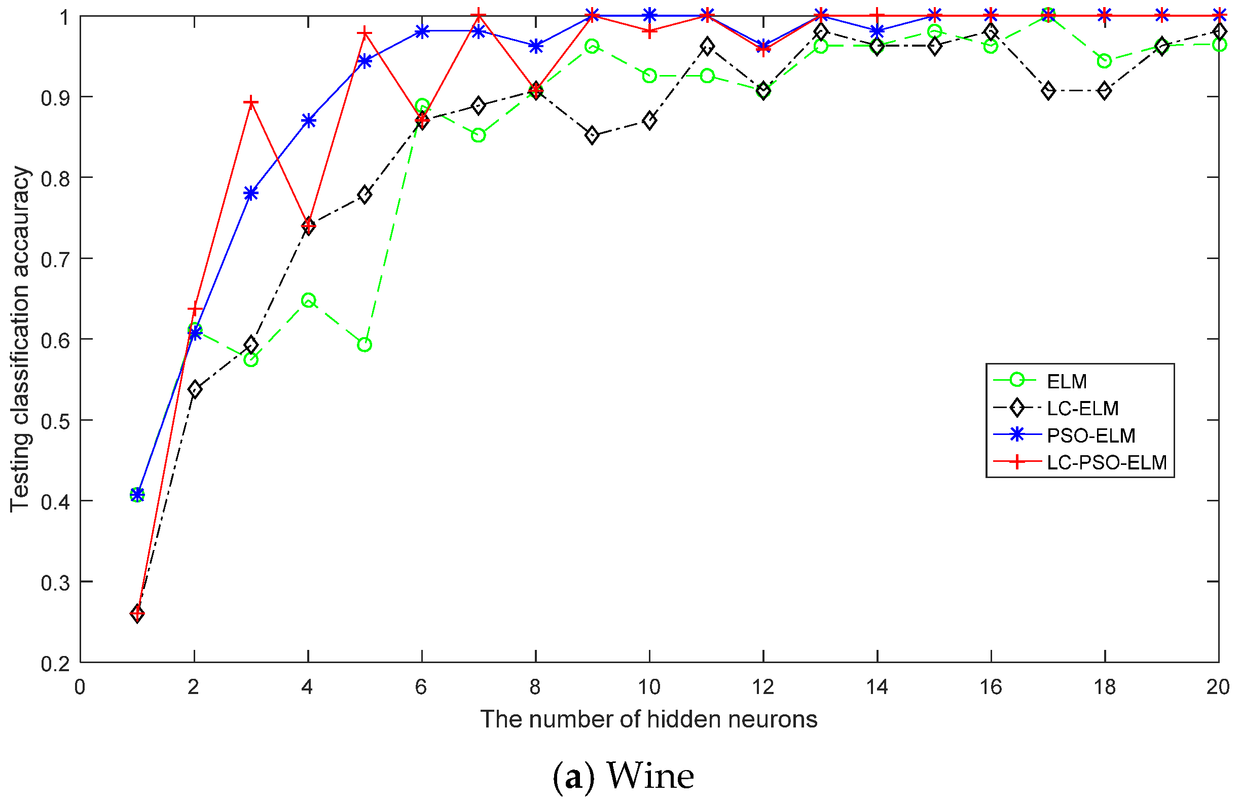
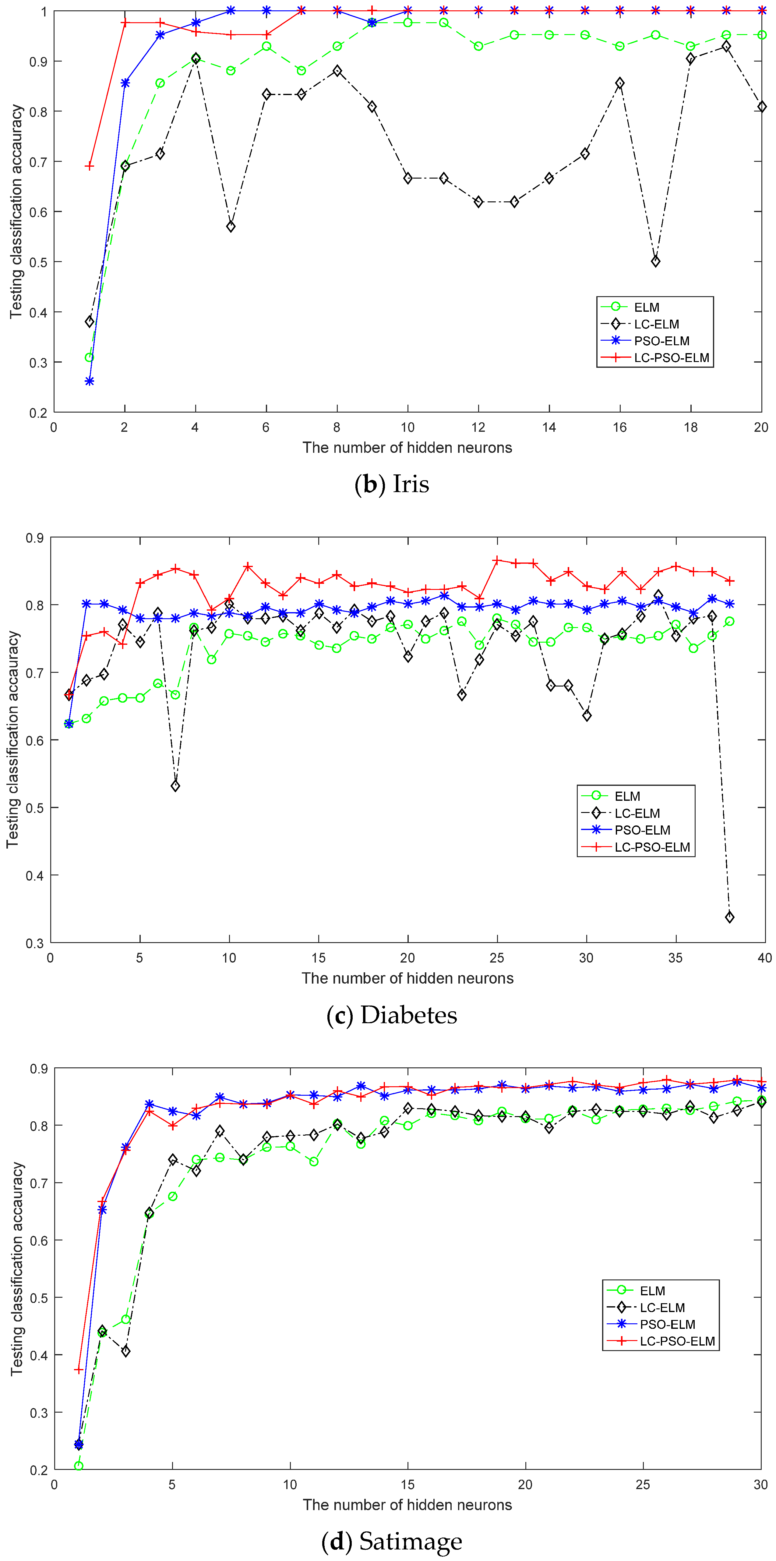
4.2. Performance Comparison of Classification Problems
- (1)
- The generalization performance of the ELM algorithm can be improved by means of the parameter optimization based on the PSO.
- (2)
- The improvement of the generalization performance has been made at the expense of the consumption of the training time of CPU for searching the optimal parameters of the model.
- (3)
- The proposed algorithm in this paper has the best generalization ability for real applications.
4.3. Performance Comparison of LC-ELM Based on Two Different Optimization Methods of DE and PSO
4.4. Performance Comparison of the LC-PSO-ELM Based on Different Fuzzy Membership Functions
5. Conclusions
Author Contributions
Funding
Conflicts of Interest
References
- Huang, G.B.; Zhu, Q.Y.; Siew, C.K. Extreme learning machine: Theory and applications. Neurocomputing 2006, 70, 489–501. [Google Scholar] [CrossRef]
- Huang, G.B.; Wang, D.H.; Lan, Y. Extreme learning machines: A survey. Int. J. Mach. Learn. Cybern. 2011, 2, 107–122. [Google Scholar] [CrossRef]
- Lv, W.; Mao, Z.; Jia, M. ELM Based LF Temperature Prediction Model and Its Online Sequential Learning. In Proceedings of the 24th China Conference on Control and Decision-Making, Taiyuan, China, 23–25 May 2012; pp. 2362–2365. [Google Scholar]
- Yu, J.; Song, W.; Li, M.; Jianjun, H.; Wang, N. A Novel Image Classification Algorithm Based on Extreme Learning Machine. China Commun. 2015, s2, 48–54. [Google Scholar]
- Wang, X.; Wang, Y.; Ji, Z. Fault Diagnosis Algorithm of Permanent Magnet Synchronous Motor Based on Improved ELM. J. Syst. Simul. 2017, 29, 646–668. [Google Scholar]
- Li, F.; Sibo, Y.; Huanhuan, H.; Wu, W. Extreme Learning Machine with Local Connections. arXiv, 2018; arXiv:1801.06975. [Google Scholar]
- Albadra, M.A.A.; Tiuna, S. Extreme Learning Machine: A Review. Int. J. Appl. Eng. Res. 2017, 12, 4610–4623. [Google Scholar]
- Sun, J. Local coupled feed forward neural network. Neural Netw. 2010, 23, 108–113. [Google Scholar] [CrossRef] [PubMed]
- Sun, J. Learning algorithm and hidden node selection scheme for local coupled feedforward neural network classifier. Neurocomputing 2012, 79, 158–163. [Google Scholar] [CrossRef]
- Yanpeng, Q. Local coupled extreme learning machine. Neural Comput. Appl. 2016, 27, 27–33. [Google Scholar]
- Mehta, R.; Vishwakarma, V.P. LC-ELM-Based Gray Scale Image Watermarking in Wavelet Domain. In Quality, IT and Business Operations; Springer: New York, NY, USA, 2018; pp. 191–202. [Google Scholar]
- Yanpeng, Q.; Ansheng, D. The optimisation for local coupled extreme learning machine using differential evolution. Math. Probl. Eng. 2015. [Google Scholar] [CrossRef]
- Hao, Z.F.; Guo, G.H.; Huang, H. A Particle Swarm Optimization Algorithm Diffrential Evolution. In Proceedings of the Sixth International Conference on Machine Learning and Cybernetics, Hong Kong, China, 19–22 August 2007; pp. 1031–1035. [Google Scholar]
- Price, K.; Price, K. Differential Evolution—A Simple and Efficient Heuristic for Global Optimization over Continuous Spaces; Kluwer Academic Publishers: Norwell, MA, USA, 1997; pp. 341–359. [Google Scholar]
- Xu, Y.; Shu, Y. Evolutionary Extreme Learning Machine—Based on Particle Swarm Optimization. In Advances in Neural Networks; Lecture Notes in Computer Science; Springer: Berlin/Heidelberg, Germany, 2006; pp. 644–652. [Google Scholar]
- Kennedy, J.; Eberhart, R. Particle swarm optimization. In Proceedings of the 1995 IEEE International Conference on Neural Networks, Perth, Australia, 27 November–1 December 1995; IEEE: Piscataway, NJ, USA, 1995; pp. 1942–1948. [Google Scholar]
- Han, F.; Yao, H.F.; Ling, Q.H. An improved evolutionary extreme learning machine based on particle swarm optimization. Neurocomputing 2013, 116, 87–93. [Google Scholar] [CrossRef]
- Du, J.; Liu, Y.; Yu, Y.; Yan, W. A prediction of precipitation data based on support vector machine and particle swarm optimization (pso-svm) algorithms. Algorithms 2017, 10, 57. [Google Scholar] [CrossRef]
- Li, B.; Li, Y.; Rong, X. A Hybrid Optimization Algorithm for Extreme Learning Machine. In Proceedings of the China Intelligent Automation Conference, Fuzhou, China, 8–10 May 2015; pp. 297–306. [Google Scholar]
- Li, B.; Li, Y.; Liu, M. A parameter adaptive particle swarm optimization algorithm for extreme learning machine. In Proceedings of the IEEE 27th Chinese Control and Decision Conference, Qingdao, China, 23–25 May 2015; pp. 1146–1160. [Google Scholar]
- Liu, C.; Wang, B.; Wang, X.; He, Y.; Ashfaq, R. An Improved Local Coupled Extreme Learning Machine. J. Softw. 2016, 8, 745–755. [Google Scholar] [CrossRef]
- Dasa, M.; Chakrabortyb, M.K.; Ghoshalc, T.K. Fuzzy tolerance relation, fuzzy tolerance space and basis. Fuzzy Sets Syst. 1998, 97, 361–369. [Google Scholar] [CrossRef]
- Rao, C.R.; Mitra, S.K. Generalized inverse of matrices and its applications. In Proceedings of the Sixth Berkeley Symposium on Mathematical Statistics and Probability, Volume 1: Theory of Statistics; University of California Press: Oakland, CA, USA, 1972; pp. 601–620. [Google Scholar]
- Li, W.T.; Shi, X.W.; Hei, Y.Q. An Improved Particle Swarm Optimization Algorithm for Pattern Synthesis of Phased Arrays. Prog. Electromagn. Res. 2008, 82, 319–332. [Google Scholar] [CrossRef]
- Li, B.; Rong, X.; Li, Y. An improved kernel based extreme learning machine for robot execution failures. Sci. World J. 2014. [Google Scholar] [CrossRef] [PubMed]
- Shi, Y.; Eberhart, R.C. A modified particle swarm optimizer. In Proceedings of the IEEE World Conference on Computation Intelligence, Anchorage, AK, USA, 4–9 May 1998; pp. 69–73. [Google Scholar]
- Ratnaweera, A.; Halgamuge, S.K.; Watson, H.C. Self-organizing hierarchical particle swarm optimizer with time-varying acceleration coefficients. IEEE Trans. Evol. Comput. 2004, 8, 240–255. [Google Scholar] [CrossRef]
- Manavalan, B.; Shin, T.H.; Kim, M.O.; Lee, G. PIP-EL: A New Ensemble Learning Method for Improved Proinflammatory Peptide Predictions. Front. Pharmacol. 2018. [Google Scholar] [CrossRef] [PubMed]
- Manavalan, B.; Shin, T.H.; Kim, M.O.; Lee, G. AIPpred: Sequence-Based Prediction of Anti-inflammatory Peptides Using Random Forest. Front. Pharmacol. 2018. [Google Scholar] [CrossRef] [PubMed]
- Box, G.E.P.; Jenkins, G.M. Time Series Analysis, Forecasting and Control; Holden Day: San Francisco, CA, USA, 1970. [Google Scholar]
- California Housing. Available online: https://www.dcc.fc.up.pt/~ltorgo/Regression/cal_housing.html (accessed on 25 October 2017).
- Blake, C.L.; Merz, C.J. Repository of Machine Learning Databases; Department of Information and Computer Science, University of California: Irvine, CA, USA, 1998. [Google Scholar]
- Li, B.; Li, Y.; Rong, X. The extreme learning machine learning algorithm with tunable activation function. Neural Comput. Appl. 2013, 22, 531–539. [Google Scholar] [CrossRef]
- Wanguo, Y.; Xu, Z.; Ashfaq, R. Comments on “Local coupled extreme learning machine”. Neural Comput. Appl. 2017, 28, 631–634. [Google Scholar]


| Problem | Dataset | Attributes | Class | Training Data | Testing Data |
|---|---|---|---|---|---|
| Regression | Box and Jenkins gas furnace data | 10 | 1 | 203 | 87 |
| Autompg | 7 | 1 | 279 | 119 | |
| Abalone | 8 | 1 | 2923 | 1254 | |
| Calhousing | 8 | 1 | 14,448 | 6192 | |
| Classification | Wine | 13 | 3 | 124 | 54 |
| Iris | 4 | 3 | 95 | 42 | |
| Diabetes | 8 | 2 | 537 | 231 | |
| Satimage | 36 | 6 | 4504 | 1931 |
| Configurations | ELM | PSO-ELM | LC-ELM | LC-PSO-ELM |
|---|---|---|---|---|
| Input weight and hidden layer biases | RN in [−1, 1] | RN in [−1, 1] | RN in [−1, 1] | NDRN (normally distributed random numbers) |
| Activation function | sigmoid | sigmoid | sigmoid | sigmoid |
| Hidden node address and window radius | -- | -- | RN in [0,1] & 0.4 | NDRN |
| Similarity | -- | -- | Wave kernel | Wave kernel |
| Fuzzy membership function | -- | -- | Equation (13) | Equation (13) |
| Algorithm | ||||||
|---|---|---|---|---|---|---|
| PSO-ELM/LC-PSO-ELM | 0.9 | 0.4 | 2.5 | 0.5 | 2 | 2 |
| Dataset Algorithms | Box and Jenkins Gas Furnace Data | Autompg | Abalone | Calhousing | Wine | Iris | Diabetes | Satimage |
|---|---|---|---|---|---|---|---|---|
| ELM | 15 | 72 | 25 | 10 | 15 | 10 | 38 | 30 |
| LC_ELM | 15 | 57 | 25 | 10 | 15 | 10 | 26 | 30 |
| PSO-ELM | 15 | 40 | 25 | 10 | 15 | 10 | 38 | 30 |
| LC-PSO-ELM | 15 | 27 | 25 | 10 | 15 | 10 | 17 | 30 |
| Algorithms | Box and Jenkins Gas Furnace Data | Autompg | ||||||
|---|---|---|---|---|---|---|---|---|
| Training Time (s) STD | Testing Time (s) STD | Training Error STD | Testing Error STD | Training Time (s) STD | Testing Time (s) STD | Training Error STD | Testing Error STD | |
| ELM | 0 | 0 | 0.0187 | 0.0214 | 0.0125 | 0.0062 | 0.0533 | 0.0866 |
| 0 | 0 | 6.9674 × 10⁻⁴ | 0.0015 | 0.0263 | 0.0197 | 0.0030 | 0.0108 | |
| LC-ELM | 0.0094 | 0.0035 | 0.0183 | 0.0262 | 0.0187 | 0.0156 | 0.0635 | 0.0885 |
| 0.0211 | 0.0075 | 0.0019 | 0.0060 | 0.0301 | 0.0255 | 0.0031 | 0.0074 | |
| PSO-ELM | 116.2472 | 0.0156 | 0.0161 | 0.0184 | 221.9707 | 0 | 0.0601 | 0.0662 |
| 2.3068 | 0.0337 | 0.0011 | 8.8292 × 10⁻⁴ | 2.8030 | 0 | 0.0018 | 0.0027 | |
| LC-PSO-ELM | 155.2323 | 0.0312 | 0.0178 | 0.0182 | 296.2370 | 0.0203 | 0.0663 | 0.0653 |
| 4.6814 | 0.0353 | 0.0017 | 0.0018 | 5.1307 | 0.0148 | 0.0027 | 0.0043 | |
| Algorithms | Abalone | Calhousing | ||||||
|---|---|---|---|---|---|---|---|---|
| Training time (s) STD | Testing Time (s) STD | Training Error STD | Testing Error STD | Training Time (s) STD | Testing Time(s) STD | Training Error STD | Testing Error STD | |
| ELM | 0.0078 | 0.0094 | 0.0756 | 0.0771 | 0.0172 | 0.0187 | 0.1441 | 0.1453 |
| 0.0198 | 0.0197 | 9.3903 × 10⁻⁴ | 0.0019 | 0.0289 | 0.0301 | 0.0030 | 0.0033 | |
| LC_ELM | 0.0593 | 0.0125 | 0.0758 | 0.0849 | 0.0577 | 0.0421 | 0.1449 | 0.1589 |
| 0.0498 | 0.0218 | 7.2119 × 10⁻⁴ | 0.0067 | 0.0255 | 0.0221 | 0.0022 | 0.0140 | |
| PSO-ELM | 308.3157 | 0.0312 | 0.0747 | 0.0761 | 486.9368 | 0 | 0.1386 | 0.1395 |
| 7.2990 | 0.0504 | 9.4281 × 10⁻⁴ | 0.0022 | 6.2410 | 0 | 0.0015 | 0.0023 | |
| LC-PSO-ELM | 1.8441 × 10³ | 0.1576 | 0.0743 | 0.0748 | 8.2110 × 10³ | 0.7653 | 0.1260 | 0.1317 |
| 55.4315 | 0.0307 | 0.0011 | 9.9337 × 10⁻⁴ | 70.2587 | 0.0689 | 0.0052 | 0.0023 | |
| Algorithms | Wine | Iris | ||||||
|---|---|---|---|---|---|---|---|---|
| Training Time (s) STD | Testing Time (s) STD | Training Accuracy STD | Testing Accuracy STD | Training Time (s) STD | Testing Time (s) STD | Training Accuracy STD | Testing Accuracy STD | |
| ELM | 0.0047 | 0.0125 | 0.9952 | 0.9741 | 0.0390 | 0 | 0.9642 | 0.9334 |
| 0.0148 | 0.0263 | 0.0068 | 0.0096 | 0.0287 | 0 | 0.0173 | 0.0219 | |
| LC-ELM | 0.0156 | 0 | 0.9911 | 0.9537 | 0.0218 | 0.0062 | 0.9779 | 0.9500 |
| 0.0255 | 0 | 0.0097 | 0.0180 | 0.0287 | 0.0197 | 0.0092 | 0.0176 | |
| PSO-ELM | 33.7149 | 0 | 0.9895 | 0.9888 | 24.1443 | 0 | 0.9880 | 0.9842 |
| 0.3132 | 0 | 0.0054 | 0.0122 | 0.7071 | 0 | 0.0078 | 0.0141 | |
| LC-PSO-ELM | 139.0843 | 0.0281 | 0.9917 | 0.9889 | 126.8756 | 0.0234 | 0.9882 | 0.9860 |
| 6.3945 | 0.0301 | 0.0099 | 0.0129 | 1.7935 | 0.0437 | 0.0060 | 0.0150 | |
| Algorithms | Diabetes | Satimage | ||||||
|---|---|---|---|---|---|---|---|---|
| Training Time (s) STD | Testing Time (s) STD | Training Accuracy STD | Testing Accuracy STD | Training Time (s) STD | Testing Time (s) STD | Training Accuracy STD | Testing Accuracy STD | |
| ELM | 0.0234 | 0.0125 | 0.8004 | 0.7835 | 0.0187 | 0.0047 | 0.8299 | 0.8248 |
| 0.0305 | 0.0263 | 0.0075 | 0.0153 | 0.0242 | 0.0148 | 0.0071 | 0.0064 | |
| LC-ELM | 0.0125 | 0.0062 | 0.7933 | 0.7779 | 0.0154 | 0.0234 | 0.8307 | 0.8238 |
| 0.0230 | 0.0197 | 0.0079 | 0.0117 | 4.9453 × 10⁻⁴ | 0.0247 | 0.0082 | 0.0081 | |
| PSO-ELM | 114.5703 | 0.0109 | 0.7937 | 0.7912 | 384.5331 | 0.0094 | 0.8513 | 0.8522 |
| 4.8491 | 0.0345 | 0.0118 | 0.0103 | 9.3345 | 0.0296 | 0.0035 | 0.0041 | |
| LC-PSO-ELM | 299.1179 | 0.0250 | 0.7966 | 0.7918 | 3.9371 × 10³ | 0.3401 | 0.8583 | 0.8685 |
| 0.6804 | 0.0168 | 0.0171 | 0.0198 | 42.8024 | 0.0161 | 0.0032 | 0.0062 | |
| Algorithms | Autompg | Iris | ||||||
|---|---|---|---|---|---|---|---|---|
| Training Time (s) | Training Error STD | Testing Error STD | Number of Hidden Neurons | Training Time (s) | Training Accuracy STD | Testing Accuracy STD | Number of Hidden Neurons | |
| ELC-ELM | 37.1688 | 0.0805 | 0.0769 | 15 | 11.8374 | 97.40 | 97.20 | 15 |
| 0.0059 | 0.0048 | 0.52 | 2.70 | |||||
| LC-PSO-ELM | 191.3243 | 0.0681 | 0.0696 | 15 | 126.8756 | 0.9882 | 0.9860 | 10 |
| 0.0035 | 0.0049 | 0.0060 | 0.0150 | |||||
| Fuzzy Membership Function | Box and Jenkins Gas Furnace Data | Diabetes | ||||||
|---|---|---|---|---|---|---|---|---|
| Training Time (s) | Training Error STD | Testing Error STD | Number of Hidden Neurons | Training Time (s) | Training Accuracy STD | Testing Accuracy STD | Number of Hidden Neurons | |
| Gaussian function | 163.3120 | 0.0175 | 0.0186 | 15 | 325.6693 | 0.7753 | 0.7637 | 17 |
| 1.7935 | 0.0010 | 3.4140 × 10⁻⁴ | 5.7551 | 0.0151 | 0.0293 | |||
| reversed sigmoid function | 155.2323 | 0.0178 | 0.0182 | 15 | 299.1179 | 0.7966 | 0.7918 | 17 |
| 4.6814 | 0.0017 | 0.0018 | 0.6804 | 0.0171 | 0.0198 | |||
| reversed tanh function | 162.3003 | 0.0242 | 0.0243 | 15 | 332.4445 | 0.7263 | 0.7133 | 17 |
| 4.7447 | 0.0024 | 0.0035 | 7.1548 | 0.0498 | 0.0668 | |||
© 2018 by the authors. Licensee MDPI, Basel, Switzerland. This article is an open access article distributed under the terms and conditions of the Creative Commons Attribution (CC BY) license (http://creativecommons.org/licenses/by/4.0/).
Share and Cite
Guo, H.; Li, B.; Li, W.; Qiao, F.; Rong, X.; Li, Y. Local Coupled Extreme Learning Machine Based on Particle Swarm Optimization. Algorithms 2018, 11, 174. https://doi.org/10.3390/a11110174
Guo H, Li B, Li W, Qiao F, Rong X, Li Y. Local Coupled Extreme Learning Machine Based on Particle Swarm Optimization. Algorithms. 2018; 11(11):174. https://doi.org/10.3390/a11110174
Chicago/Turabian StyleGuo, Hongli, Bin Li, Wei Li, Fengjuan Qiao, Xuewen Rong, and Yibin Li. 2018. "Local Coupled Extreme Learning Machine Based on Particle Swarm Optimization" Algorithms 11, no. 11: 174. https://doi.org/10.3390/a11110174
APA StyleGuo, H., Li, B., Li, W., Qiao, F., Rong, X., & Li, Y. (2018). Local Coupled Extreme Learning Machine Based on Particle Swarm Optimization. Algorithms, 11(11), 174. https://doi.org/10.3390/a11110174