3.2. Mechanical Response
In the stress-controlled numerical implementation used here to examine the mechanical response of graphene, we compute the resulting strain due to the fixed force applied at the appropriate edge atoms. The uniaxial strain
is obtained through the strain of the central row of the graphene sheet when the stress is applied in the armchair direction, while it is calculated by the average strain on the two central columns of the sheet in case of stress in the zigzag direction (see
Figure 1).
indicates the strain corresponding to temperature
T.
In the zero-temperature case, i.e., where
K, the uniaxial strain
is determined through the relative change in the length of the central row (two central columns) of graphene subjected to a given applied stress in the armchair (zigzag) direction with respect to the length of the central row (columns) in the unstrained equilibrium configuration shown in
Figure 1. These measurements are taken in the central region of the lattice, as mentioned at the end of the previous subsection. For any length computations discussed here, a horizontal (vertical) length is measured as the difference of the
x (
y) coordinates of the edge atoms considered. The stress–strain response is obtained in this way at 0 K.
When the temperature of the system is raised at finite values, by adding energy to the equilibrated graphene, the lattice stretches and compresses in an oscillatory manner. The details of these oscillations depend on the temperature and the applied stress and will be investigated in the future. In this case, one has to take into account that the strain measurement is now exhibiting temporal oscillations. Since we consider 10-20 different realizations of the randomly inserted initial energy distribution, we register the average, over these realizations, strain in time , noting that the aforementioned oscillations are in-phase in the different realizations.
For evaluating the strain
of a uniaxially loaded graphene sheet at finite temperatures, a reference length
corresponding to zero stress
at the particular value of
T is needed. This reference length accounts for thermal effects on the initial configuration, and it is obtained by calculating the average, over realizations and time, of the length of the central row, or columns, of the sheet in the absence of a load. Then, when a stress is applied, the time evolution of strain in a particular realization is determined as the relative change in the length with respect to the reference length
where
is the length at time
t of the central row or the average length of the two central columns depending on the direction of the applied uniaxial load.
In
Figure 3, we highlight the behavior of
for various values of stress
in the zigzag direction at three distinct temperatures
T, which are indicated by different colors. An increase in temperature leads to an increase in the amplitude of strain oscillations as well as in the average strain. The latter is obtained as the average over both realizations and time,
, and it is indicated by the dashed horizontal lines of different colors depending on the temperature in
Figure 3. The average strains
(red horizontal dashed lines) about which the
K curves oscillate are higher than the
(blue horizontal dashed lines) of the
K curves in all cases of different stress. However, these differences are larger for absolute values for larger stresses.
We have validated that if one follows an alternative path on the plane by first giving initial energy to the system and then applying forces at the edges, practically identical average strains are obtained. However, our approach is much more efficient because the temperature is accurately controlled and, more importantly, the system reaches thermal equilibrium significantly faster; in the alternative method, the equilibration takes orders of magnitude longer.
Calculating the average strain
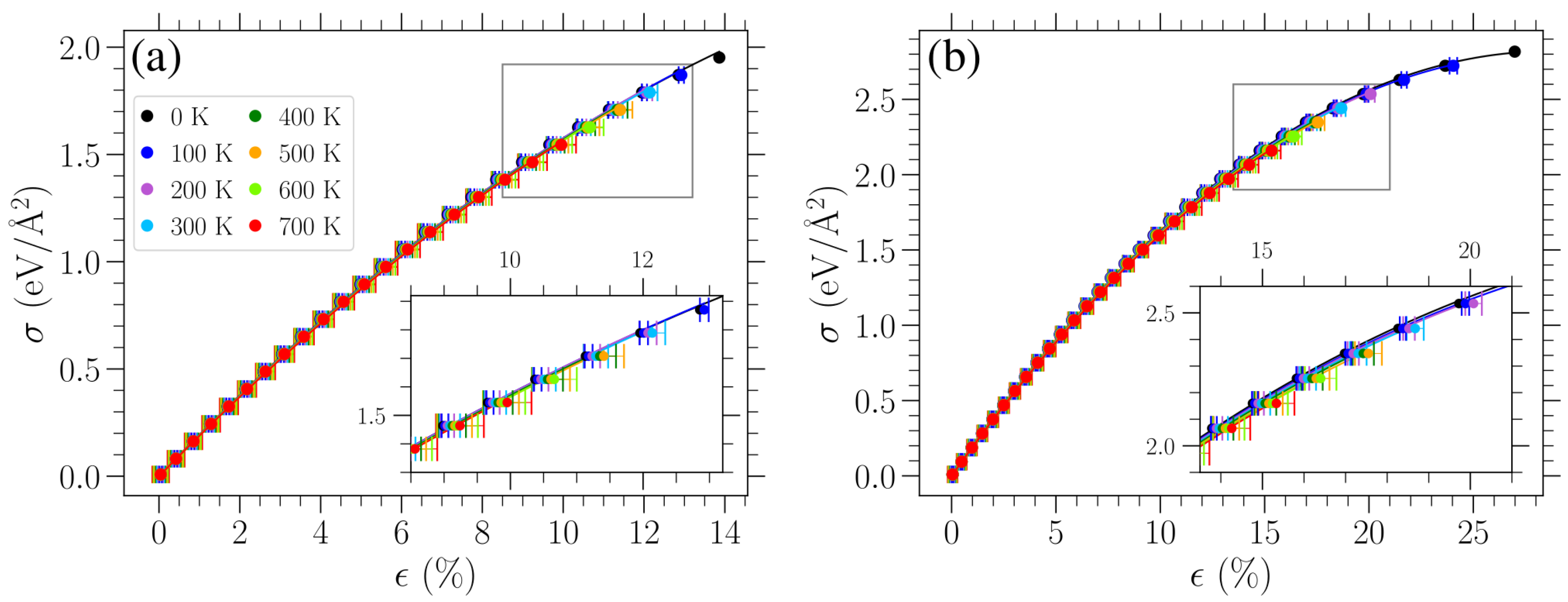
, as mentioned above, allows one to obtain the mechanical response of planar graphene at different temperatures. Stress–strain curves for uniaxial tensile loads in the armchair and zigzag directions are presented for various temperatures in
Figure 4. Despite the small differences, one can see for larger stresses that the average strain is a bit further to the right for the higher-temperature cases. The error bars indicate the standard deviation of the average strain measurement. As one can also deduce from
Figure 3, the standard deviation is higher for higher temperatures. This is highlighted via the insets in each panel, where a close-up of the data points and error bars is presented for the region, which is indicated by the gray rectangle in each panel. When examined close-up, it is easier to see that the lengths of the error bars increase with temperature.
We have checked the accuracy of the presented strain measurements when more realizations or longer time windows are considered. In particular, the obtained strain values differ in the 3rd significant digit at most when the number of realizations is increased or the length of the time window is doubled.
Since, at finite temperatures, strain is measured with respect to the averaged oscillating length
due to thermally induced vibrations of the unstrained sheet, the stress–strain curves pass through the origin of
Figure 4, as expected. From
Figure 4, we can see that the temperature has a relatively small effect on the stress–strain response, at least for the values of
T considered here, apart from the significant reduction in the fracture point. For small stresses, the achieved strain is practically the same for the two directions of applied stress, while the strong directional dependence at large stresses has already been well established in previous investigations [
5,
12,
20,
28].
The stress–strain response can be described by the nonlinear relation [
12]
where
is the applied uniaxial stress,
is the corresponding strain,
is the 2D Young’s modulus, and
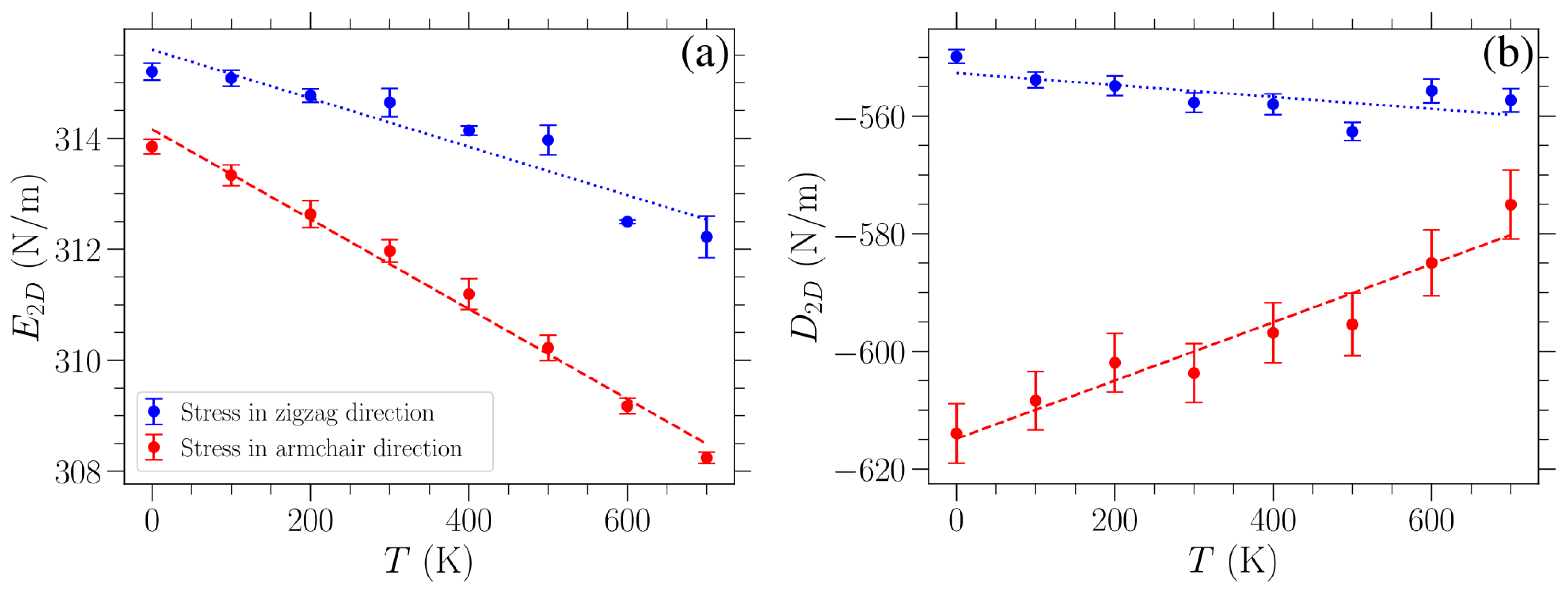
is the 2D third-order elastic modulus. For each temperature examined and both directions of applied stress, we first obtained the value of Young’s modulus using the linear response at small stress/strain, and then we fit the data presented in
Figure 4 with Equation (
7) to determine the third-order elastic modulus. The computed values of
and
are plotted in
Figure 5 as a function of temperature for applied stress in either the armchair (red points) or the zigzag (blue points) direction. The error bars on these points indicate one standard deviation of the fitted parameters under the observed covariance of the fit. A linear variation can roughly approximate the obtained temperature dependence of these elastic moduli. Linear fittings of the corresponding data are indicated by the dashed red (dotted blue) line for stress in the armchair (zigzag) direction.
The Young’s modulus
(
Figure 5a) appears to decrease almost linearly with an increasing temperature, albeit only by a relatively small amount, which is consistent with other results in the literature [
7,
33,
41]. In particular, the linear fitting of these data for stress in the armchair direction leads to a variation in
with a slope of
(N/m)/K, while for stress in the zigzag direction, the slope is
(N/m)/K.
The decrease in the Young’s modulus with temperature is often given in the literature as a percentage change over the investigated range of temperatures. To ensure we make a superior direct quantitative comparison, we present our results along with existing ones in the literature as percentage change per 100 K. In our case, the Young’s modulus decreases by
K and
K for stress in the armchair or the zigzag direction, respectively. Combined density functional theory and quasi-harmonic approximation calculations in Reference [
33] yielded a
decrease by
K over the range from 0 K to 1000 K. Molecular dynamics was used in Reference [
7] for investigations, at 300 K, 500 K, and 700 K, of graphene lattices of different aspect ratios consisting of 1886 atoms.
was found to decrease by
K,
K, and
K (
K,
K, and
K) for strain in the armchair (zigzag) direction, where the three different values correspond to graphene aspect ratios of 1.97, 1.44, and 1.01 (1.95, 1.45, and 0.99). We note that our lattice has an aspect ratio of 1.72. Molecular dynamics simulations in Reference [
14] resulted in a
decrease by
K over a temperature range of 300 K to 2000 K for strain applied in the armchair direction. Finally, in Reference [
41], a reduction in
between
K and
K was obtained for temperatures ranging from 0 K to 1600 K, where the varying reduction depends on the different parameterizations of the model used, thus affecting the Young’s modulus value at
K.
The calculated Young’s modulus
at 300 K is in good agreement with values reported in experimental studies conducted at room temperature [
1,
2,
3]. In particular, our findings, namely, 315 N/m and 312 N/m for loading in the zigzag and armchair directions, respectively, are consistent with the Young’s modulus reported in Reference [
1] (340 ± 50 N/m), [
2] (300 to 340 N/m), and [
3] (350 ± 100 N/m).
We can observe from
Figure 5b that the
values are consistently higher for strain in the zigzag direction than for the other direction. This is congruent with the fact that the graphene sheet is more resistant to stress in the zigzag direction. When stress is exerted in the armchair direction, one third of all the bonds are parallel to the direction of strain, and hence these bonds exhibit maximal stretching in the sheet. Taking into account the respective angle deformations, there is generally higher strain for the same stress in this case as compared to loads in the zigzag direction. As the Young’s modulus is almost the same in these two cases, there is a lower
modulus (i.e., higher absolute values) for stresses in the armchair direction. The different strains for a given stress in the two perpendicular loading directions discussed here can be seen when comparing the panels of
Figure 4, where the curves for stress in the armchair direction lie further to the right than when the stress is applied in the zigzag direction, indicating higher strains for the same stress. Regarding the temperature variation of
, different trends are exhibited when the stress is in the zigzag or armchair direction. A linear fitting of the
data points results in a slope
(N/m)/K for strain in the armchair direction and
(N/m)/K for strain in the zigzag direction. The value of
increases by
K (decreases by
K) for strain in the armchair (zigzag) direction over the temperature range from 0 K to 700 K.
Finally, we estimate the graphene’s fracture strength
and failure strain
for different temperatures
T. The former is obtained by using the highest tested value of stress
that does not lead to failure of the graphene sheet. Its error bar is provided by the step we used when increasing the tested
values, which are evenly spaced. These results are presented in
Figure 6a, where an almost linear decrease in fracture stress with temperature is shown. A linear fitting of these data points is indicated with a dashed red (dotted blue) line for stress in the armchair (zigzag) direction. The slope of the linear fitting of the
data is
(N/m)/K for stress in the armchair direction and
(N/m)/K for stress in the zigzag direction.
Such a linear dependence of the fracture strength on temperature is in accordance with existing results. In particular, we estimate that, based on the MD study on graphene loaded in the armchair direction reported in Reference [
9], fracture strength decreases with temperature at a rate of
(N/m)/K, which is in very good agreement with the slope obtained in our work for the same direction. Molecular dynamics simulations were also used in Reference [
40], and the presented temperature dependence of the fracture stress decreased linearly with a slope of
(N/m)/K. However, the loading direction was unclear in the cited case. In another MD investigation, where the stated loading direction was the armchair direction, the corresponding slope was found to be
(N/m)/K [
14]. Lastly, Reference [
24] employed a combination of machine learning and MD simulations with the Tersoff potential. In that study, the fracture strength decreased linearly with temperature, exhibiting a slope of
(N/m)/K for loading in the zigzag direction, whereas for loading in the armchair direction, a bilinear behavior is observed: the slope is initially
(N/m)/K but becomes steeper above 500 K, thus representing the only non-linear trend reported in the literature.
The failure strain,
, at different temperatures has been estimated through the value of fracture stress by solving for
in Equation (
7). To this end, the known value of
, as well as the fitted values of
and
describing the stress–strain curve at the given temperature, has been used. In this case, the error bars were determined by converting the corresponding extreme values of stress,
, to strain (via Equation (
7)), and then choosing the maximum absolute difference from
. These results are shown in
Figure 6b, where again a linear fitting of the data is indicated with a dashed red (dotted blue) line for stress in the armchair (zigzag) direction. The linear fitting of the
data points leads to a slope
% strain/K for stress in the armchair direction and
% strain/K for stress in the zigzag direction. We can further compare these slopes to existing results by estimating the slopes of the failure strain versus temperature data reported in the literature. For uniaxial loading in the armchair direction, in Reference [
9], a slope of
% strain/K was estimated, which is in very good agreement with our result. A slope of
% strain/K was estimated for the results presented in Reference [
40], where, as noted above, the loading direction was unclear. Finally, the corresponding slope for strain applied in the armchair direction was
% strain/K in Reference [
14].
The fracture stress reported in the experimental study conducted in Reference [
1] is
N/m. We obtained an intrinsic strength of
N/m (
N/m) and a fracture strain of
(
) for loading in the zigzag (armchair) direction at 300 K. We note that our results are in good agreement with the intrinsic strength and fracture strain values reported elsewhere, which additionally allow out-of-plane deformations of the material. Specifically, MD simulations carried out at 300 K using the AIREBO potential yield, for loading in the zigzag direction, intrinsic strengths of around
N/m and fracture strains between
[
3,
5]. For loading in the armchair direction, Reference [
47] conducted MD simulations using the REBO force field at 300 K, obtaining a fracture strain of
at a stress of
N/m, while Reference [
5], who used AIREBO, reported an intrinsic strength of
N/m and a fracture strain of
.
The results shown in
Figure 6 indicate that graphene fails at lower applied stress/strain as temperature increases. This is reasonable since, as can be clearly seen from
Figure 3, for the stress-controlled simulations considered here, the sheet achieves higher strains over the course of its oscillations by increasing temperature. As a result, for fixed stress, the bonds between neighboring atoms experience greater stretching at higher temperatures and therefore are more likely to break, causing failure of the material due to the increase in the maximum deformation of the lattice. Moreover, graphene can tolerate greater loads in the zigzag direction in the whole temperature range investigated here, as implied by the results in
Figure 6, where the values of fracture strength and failure strain are consistently lower for stress in the armchair direction (red data points) as compared to stress applied in the zigzag direction (blue data points). In contrast to the relatively stronger temperature dependence of the fracture strength and failure strain, the Young’s modulus variation shown in
Figure 5a exhibits a much smaller relative change, implying that the influence of thermal effects on the stiffness of graphene is less significant, at least within this temperature regime.
3.3. Bond Length and Bond Angle Distributions
In order to analyze the effects of temperature and stress on the distributions of the lengths and angles of the bonds, we first distinguish the two types of bond lengths, denoted by
A and
Z, and the two types of angles, indicated by
and
, as illustrated in
Figure 1. The
A bonds are in the armchair direction. The
Z bonds alternate symmetrically in the zigzag direction and both exhibit identical deformations at 0 K when a uniaxial stress is applied in the high-symmetry zigzag or armchair directions. The angles
and
represent the bond angles formed between two consecutive
Z bonds and between an
A and a
Z bond, respectively. They always respond oppositely under an applied stress due to the geometry of the system and the constraint
.
When a load is applied at zero temperature, due to the absence of fluctuations and the static nature of the strained sheet, there is no variability in the two types of bond lengths and angles, and their distribution is delta-peaked. Approximate expressions for the strain dependence of bond lengths
A and
Z and angles
and
were provided in Reference [
42]. With the indices
a or
z used to indicate a load applied in the armchair or zigzag direction, respectively, these expressions read as follows:
and
while for stress in the zigzag direction,
and
In Equations (
8), (9), (
12) and (13), the bond lengths
A or
Z are given in Å, and the zero-temperature strain
is expressed as % strain. Similarly, in Equations (
10), (11), (
14) and (15), the bond angles
and
are provided in degrees, and
should be given again as a percentage strain. The distributions of bond lengths (angles) in bulk graphene at
K are given by double singular peaks at the locations provided by the above pairs of relations for the bond lengths (angles), depending on the direction of the loading for different values of the applied uniaxial strain.
In order to reveal the influence of temperature on the bond length and angle distributions, we registered all the fluctuating bond length and angle values during the system’s evolution in our measurement window and obtained normalized distributions for different amounts of stress/stain at various temperatures. In particular, we created a distribution for each realization by allocating all the measured bond lengths (angles) to fine-grained bins with a width of
Å (
). The resulting distributions were normalized and then averaged over the different realizations in order to obtain the final distribution for each case. It is worth noting that the size of the error bars, indicating one standard deviation of this averaging computation over the different realizations, is negligible and hence not included in the plots of the distributions presented below. We emphasize again that we consider the central region of the sheet for collecting our data, as mentioned at the end of
Section 3.1.
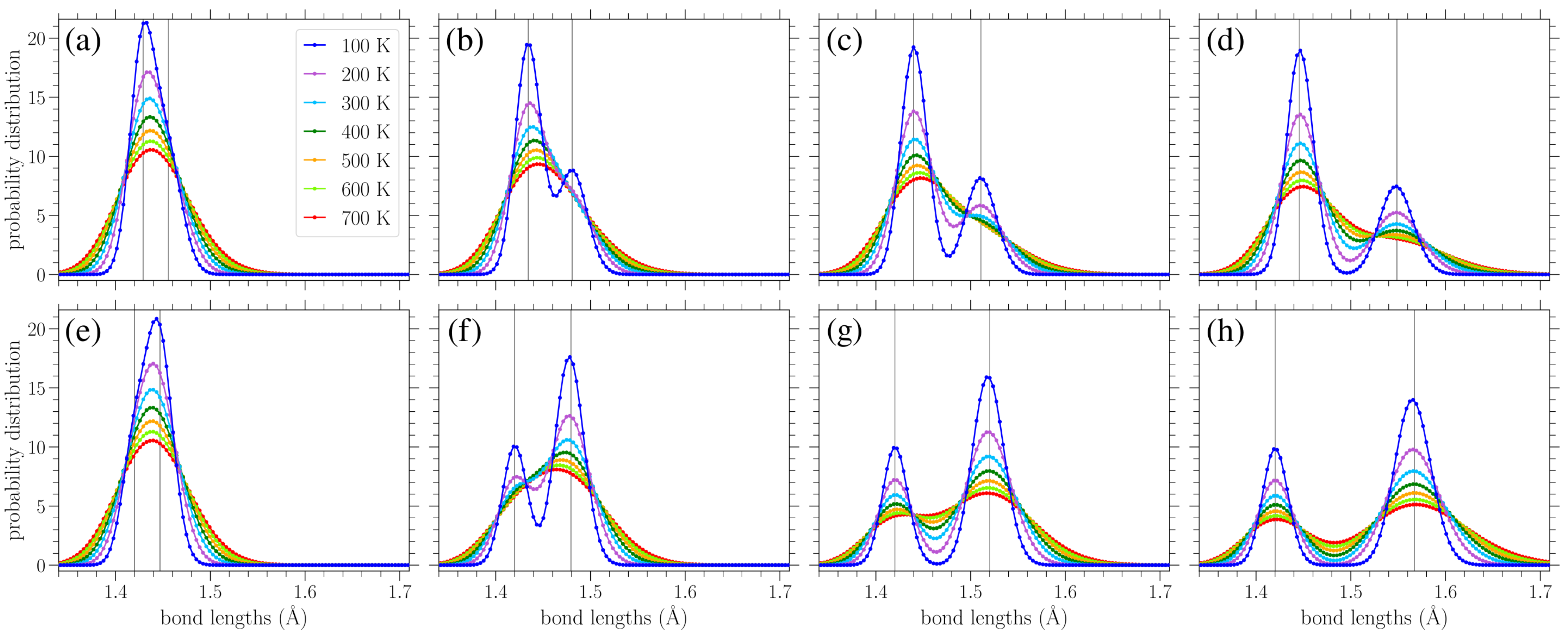
In
Figure 7a–d, we show the normalized bond length distributions for increasing values of stress applied in the armchair direction. In
Figure 7e–h, the applied load is in the zigzag direction, and the stress increases from (e) to (h) too. When there is no loading, i.e.,
, at finite temperatures, the distributions are simply normal distributions with the variance linearly increasing with temperature (see
Section 3.3.1). Increased temperature leads to larger fluctuations in the lattice, resulting in a wider spread of the observed bond lengths. In the presence of uniaxial loading, for the smaller values of stress presented in
Figure 7a,e, there is a slight skewing of the distributions. As the stress is increased, the single peak splits into two peaks that are gradually separated more and more, as can be clearly seen from the plots corresponding to lower temperatures, due to the increased separation of the
A and
Z bond length values (see Figures 2 and 3 in Reference [
42]). However, the increase in temperature leads to the merging of these two peaks due to their broadening. The centers of the peaks correspond to the zero-temperature values of the two types of bond lengths for each different direction of the applied stress, as given in Equations (
8), (9), (
12) and (13).
Since there are twice as many
Z-type bond lengths as
A-types, the highest peak in each distribution in
Figure 7 mostly encompasses the lengths of the
Z-type bonds. Thus, we can see that for stress applied in the armchair direction (
Figure 7a–d), it is the
A bonds that achieve greater lengths (the lower peak, further to the right), while the
Z bonds exhibit smaller extension. In contrast, for stress applied in the zigzag direction (
Figure 7e–h), the
Z bonds achieve greater lengths (the taller peak is to the right in the distributions), while the centers of the smaller peaks remain near
Å, in accordance with Equation (
12) and the corresponding broadening due to thermal effects. The fact that all bonds stretch for stress applied in the armchair direction, but only the
Z type bonds (two-thirds of all the considered bonds) are extended for a load in the other direction [
42], proves that the gap between the two peaks is more pronounced for stress applied in the zigzag direction.
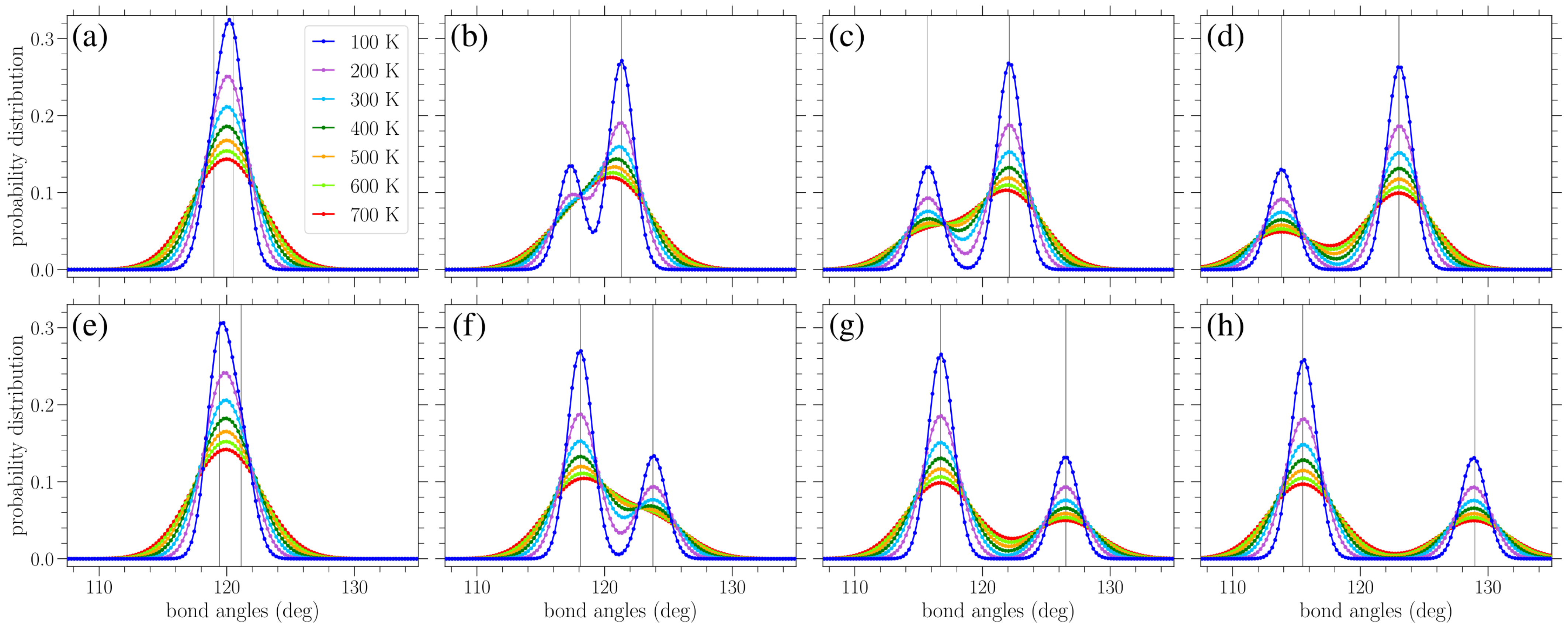
In
Figure 8, results similar to those given in
Figure 7 are presented, but for the distribution of bond angles. At zero strain, normal distributions centered about the equilibrium angle of
were obtained for finite temperatures, with a variance increasing with temperature (see
Figure 9b below). Again, we see the gradual peak splitting due to increased stress, while increasing the temperature leads to the broadening and merging of these peaks. The highest peak in the bond angle distributions corresponds to the
-type angles, since there are twice as many
angles as
angles. For stress in the armchair direction (
Figure 8a–d), the
angles decrease, while the
angles increase. The reverse is true when the stress is applied in the zigzag direction (
Figure 8e–h). Also, in this case, the peaks of the distributions are centered about the zero-temperature
and
values, as given in Equations (
10) and (11) or (
14) and (15), depending on the direction of the applied stress.
3.3.1. Analytical Expressions for the Bond Length and Bond Angle Distributions
We now present approximate analytical expressions for the bond length and angle distributions, as shown in
Figure 7 and
Figure 8, in order to describe the dependence of graphene’s structural properties on stress and temperature. Based on the results discussed in the previous subsection, we note that the obtained distributions appear to approximately be given through the combination of two normal distributions, where the means of these normal distributions correspond to the values of the two types of bond lengths, or angles, found for each stress at zero temperature. The variance of these normal distributions is induced by thermal fluctuations, while the difference in peak heights is related to the fact that there exist twice as many of one type of bond length (or angle) as the other.
As there exist approximate expressions for the equilibrium bond lengths and bond angles as a function of the applied strain at K (see Equations (8)–(15)), the explicit dependence of variance on temperature remains to be determined. This will be achieved by numerically evaluating the effects of temperature on the normal distributions of the bond lengths and bond angles for the unstrained graphene sheet. The results of these calculations will be compared with analytical estimates of the variance through the Boltzmann distribution, using a second-order approximation on the relevant potential energy terms describing bond stretching and angle bending.
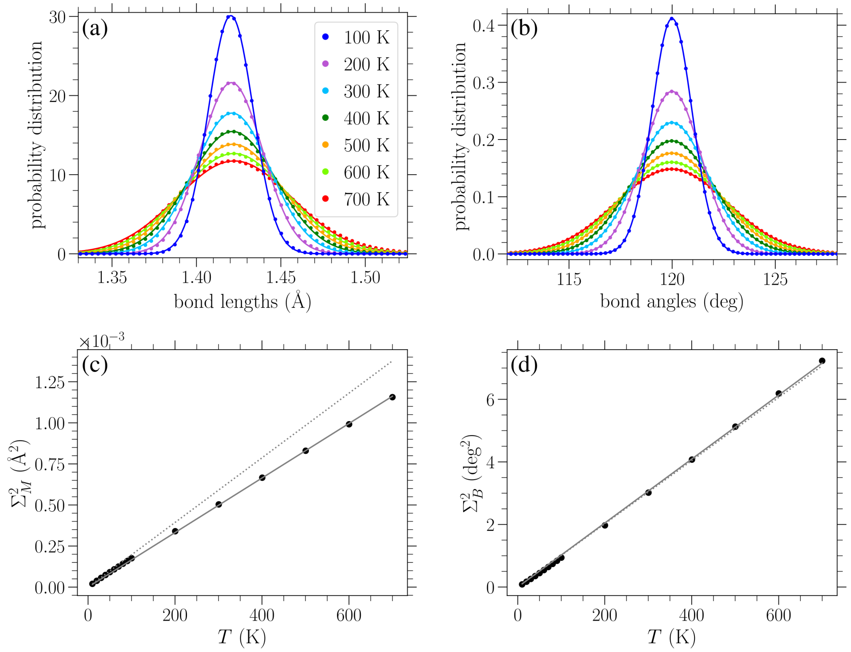
Performing a Gaussian-curve-fitting procedure for the numerically obtained distributions of the bond lengths and bond angles at zero applied stress for various temperatures (as shown in
Figure 9a,b, respectively), we computed the corresponding variances and mean values. The dependence of these variances on temperature is indicated by filled circles in
Figure 9c,d for the bond length and angle distributions, respectively. Solid lines in the remaining plots denote a linear fitting of the data. It is worth noting that the mean of the bond length distribution slightly increases with temperature too due to the soft Morse potential describing bond stretching. However, incorporating this small variation in the mean value with temperature does not practically affect the results discussed below. The mean of the bond angle distribution does not change with temperature, as expected due to the equality of the
and
angles in the unstrained graphene and their constrained sum.
A linear fitting describes the dependence of the variance
of bond length distributions on temperature
T:
with
Å
2/K (solid line in
Figure 9c). Similarly, the numerically found variances
for the bond angle distributions are well described by
with
deg
2/K (solid line in
Figure 9d).
The proportionality of these variances with temperature can be derived through the Boltzmann distribution when a quadratic approximation of the corresponding potential energy is considered. In particular, according to the second derivative of the Morse potential of Equation (
1),
the second order approximation of the bond-stretching energy term about the equilibrium
reads
. Using this approximation, the corresponding Boltzmann distribution
results in a normal bond length distribution of the form
centered about the mean
with a variance
which gives
(Å
2/K)
when the parameters of the Morse potential are substituted.
Following a similar approach to estimate the variance of the bond angle distributions for different temperatures, we consider the second-order approximation of the potential
, Equation (
2), about
, given by
(when angles are measured in degrees). Note that due to the constraints on the sums of the bond angles around a particular atom and on the sums within hexagonal rings, just one angle can not be varied alone. When an angle slightly varies from the equilibrium value, at least three other angles should also change. Thus, multiplying the linearized angle-bending energy in the Boltzmann distribution by a factor 4, we eventually find the variance (in squared degrees), about the mean
, of the bond angle distribution
which results in
(deg
2/K)
, using the value of
d.
The dotted lines in
Figure 9c,d correspond to the analytical expressions of Equations (
19) and (
20), respectively. We can see from
Figure 9c that the analytically obtained slope of Equation (
19) is somehow larger than the corresponding numerical value of Equation (
16) (the relative difference is less than 20%). Concerning the variance of the bond angle distributions,
Figure 9d shows an excellent agreement between the analytically and numerically obtained slopes, exhibiting a relative difference of less than 1%. One reason for the quantitative disparity between the analytical prediction and numerical determination of the slope of the linear temperature dependence of the variance of the bond length distributions, but not for the angle distributions, may be the fact that the second-order approximation of the angle-bending potential
of Equation (
2) is valid for a wide range of angles (see Figure 2 in Reference [
12]). However, due to the highly anharmonic nature of the Morse potential
, Equation (
1), at the same energy scales (see Figure 1 in Reference [
12]), the second-order approximation about
is only valid when very close to
.
By combining the numerically determined variances for different temperatures and the known bond length and angle mean values as a function of the applied stress/strain, analytical approximate expressions for the bond length and angle distributions can be derived. Regarding the bond length distributions, an additional issue should be taken into account when the numerically determined variances from Equation (
16) will be used. In particular, the relation between variance and temperature should be scaled according to the behavior of
(Equation (
18)) at the mean of the corresponding peak of the distribution since bond lengths even further away from
are encountered once stress is applied to the system and the second derivative of the Morse potential varies significantly with
r. Given that, analytically, the variance equates to
, when close to
, we multiply the numerically determined variance from Equation (
16) by the scaling function
where
r is the known mean of the peak of interest in the distribution, provided by either Equations (
8) and (9) or Equations (
12) and (13) depending on the loading direction.
As a result, the bond length distribution for a given applied stress/strain and temperature
T can be approximated by the relation
where
A and
Z are functions of the applied stress/strain, determined in Equations (
8) and (9) or Equations (
12) and (13), for stress in the armchair or zigzag direction, respectively,
is given in Equation (
16), and
is yielded by Equation (
21). The factor of 2 in the second term is present because there are twice as many
Z bonds as
A bonds. Division by 3 is employed for normalizing the distribution. Note that the quantities
A and
Z are provided by the corresponding zero-temperature relations in Equations (
8), (9), (
12) and (13) as a function of strain
. If they are needed as a function of stress
, the stress–strain relation of Equation (
7) should be used to change the variable of the applied load.
For the bond angle distributions, the subtlety mentioned above concerning the scaling function is not needed since the second derivative of the angle-bending potential, Equation (
2), is the same everywhere regardless of the angle value at the peak of the distribution. Therefore, the angle-bending distributions can be approximated by the expression
where
and
are determined by the applied stress/strain from Equations (
10) and (11) or (
14) and (15), depending on the loading direction, and
is provided by Equation (
17). The factor 2 in the second term is present because there are twice as many
angles as
angles, and division by 3 normalizes the distribution. If the loading is given through the value of stress, Equation (
7) can be also used.
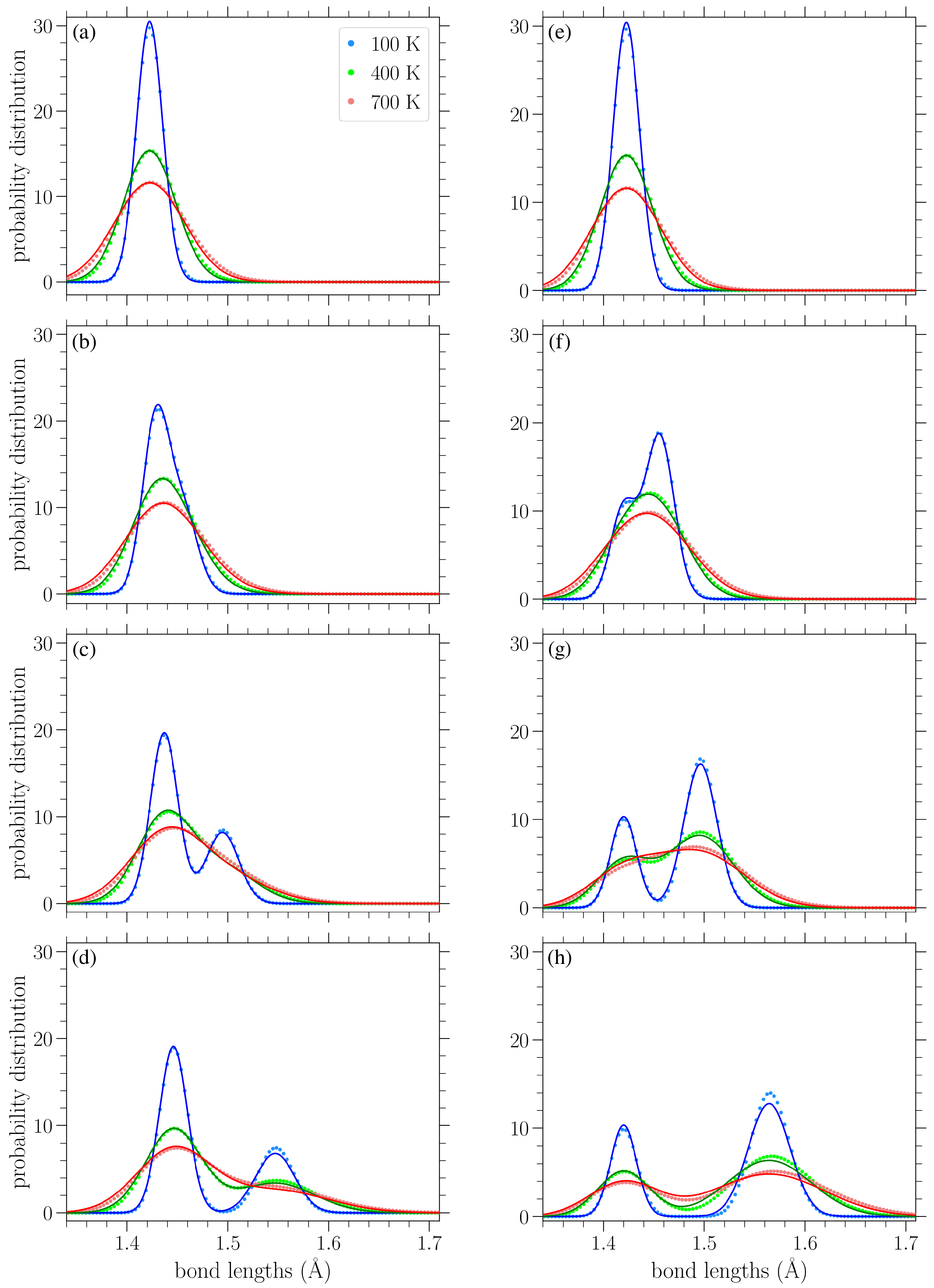
The circles in
Figure 10 present the numerically computed bond length distributions at various applied stresses and temperatures, while the solid lines correspond to the curve
from Equation (
22).
Figure 11 contains similar results, but for the bond angle distributions. These plots show that the analytical expressions presented above provide a reasonable description of the bond length and angle distributions in strained graphene at various temperatures, at least up to the values considered here. In
Figure 10, at the larger values of applied stress and lower temperatures, the analytical distribution
of Equation (
22) underestimates the longer-bond (second) peak of the numerically obtained distributions (
Figure 10d,g,h).
Figure 10h shows the greatest deviation of the analytical expression from the numerical data at the right-hand peak of the lowest temperature at
K; in this case, the difference is 8.7%. From the plots of
Figure 11, we can see that the analytical expression
(Equation (
23)) describes the data quite well, apart from small discrepancies at the heights of the taller peak at the lower temperatures depicted and for the smaller values of stress.
Figure 11a shows the biggest deviation for the
K case, where the value of the analytical expression is 4.1% below that of the numerical data. In any case, both expressions of Equations (
22) and (
23) provide a useful analytical description of the underlying structural properties of the strained graphene at finite temperatures.


