

Experimental Investigation of Steel Bar Corrosion in Recycled Plastic Aggregate Concrete Exposed to Calcium Chloride Cycles
 , ,
, ,  , , ,
, , , 

Highlights
- Partial substitution of natural aggregates with recycled plastic granules.
- Compressive strength decreased but fracture energy absorption increased.
- Corrosion behaviour study with wet/dry exposure to calcium chloride solution.
- Hydrophobicity of plastic granules decreased chloride’s diffusion tendency.
- Corrosion of rebars depended on amount and distribution of plastic granules.
Abstract
1. Introduction
2. Materials and Methods
2.1. Concrete Production and Preparation of Specimens
2.2. Mechanical Tests
2.3. Chloride Exposure
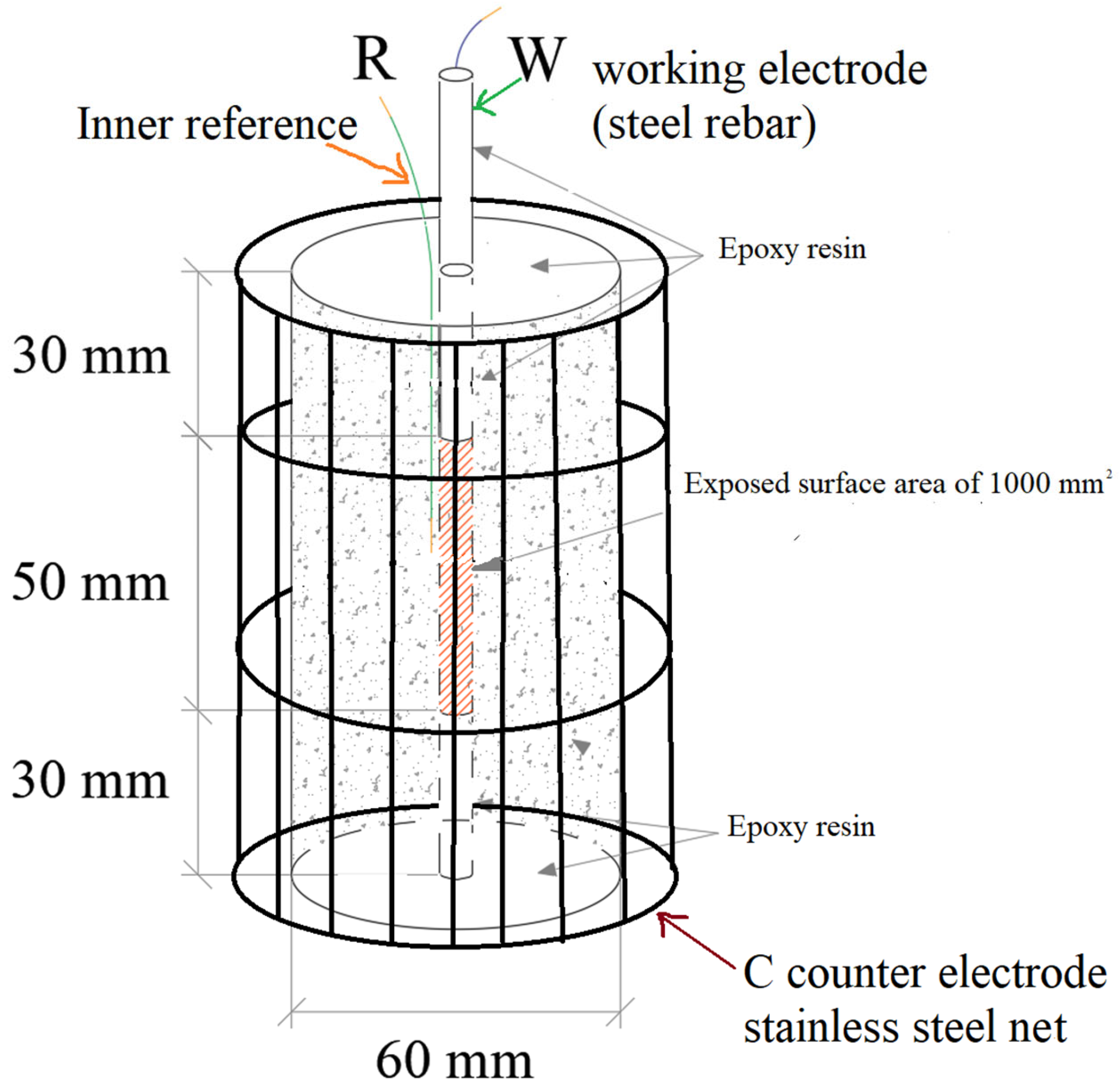
2.4. Electrochemical Tests
3. Results and Discussion
3.1. Mechanical Characterization
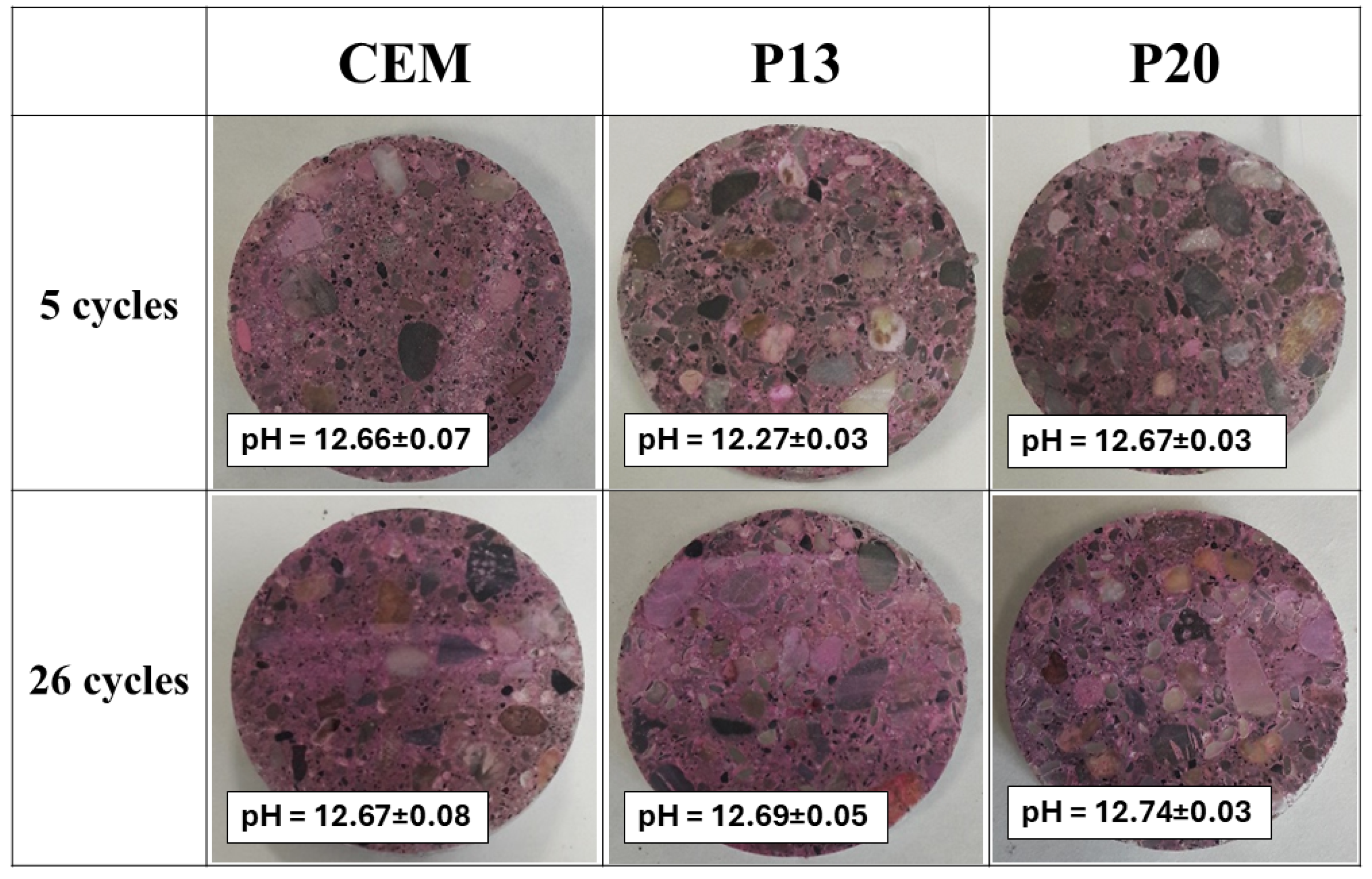
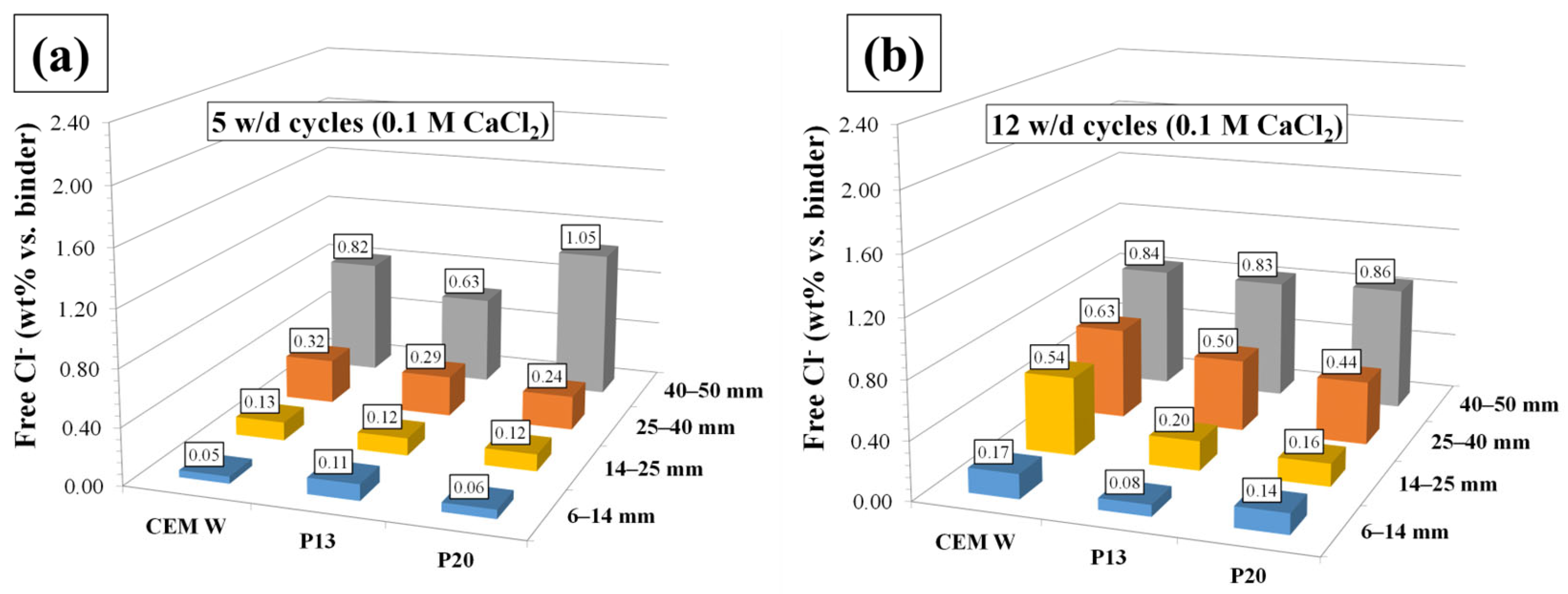
3.2. Analytical Measurements During the Exposure
3.3. Electrochemical Tests
3.3.1. Linear Polarization Resistance Measurements
3.3.2. Electrochemical Impedance Spectroscopy
3.3.3. Polarization Curves
4. Conclusions
- Partial replacement of natural aggregate with plastic granules results in a decrease in both compressive strength and tensile (splitting and flexural) strength, even if the latter appears less influenced than compressive strength by the addition of plastic granules. In more detail, P13 and P20 show a compressive strength reduction of about 25% and 45%, respectively, compared to CEM, while the tensile strength decreases by approximately 15% and 30%. On the contrary, a significant increase in fracture energy is observed (about 30% for P13 and 95% for P20 compared to CEM), indicating an enhanced capacity to absorb and redistribute tensile forces. These results underline the role of plastic aggregates in transforming the failure mode of concrete, providing valuable insights into improving its brittle behavior.
- Wet and dry exposure to chlorides for 365 days does not adversely affect the mechanical strength of plastic-added concrete.
- The hydrophobic nature of plastics granules resulted in higher concrete flowability. In more detail, the mixtures P13 and P20 required 50% and 62% less superplasticizer, respectively, than CEM to reach the same slump values. Moreover, this same characteristic of plastics allows to slow the tendency to migration of chlorides towards the reinforcement bar, with average total chloride concentrations (after 26 w/d cycles) of 0.40 and 0.49 (wt% vs. binder) for P13 and P20, respectively, compared to what was observed in the reference concrete with a concentration of 0.79 (wt% vs. binder). The amount and distribution of the plastic granules, influencing the porosity of concrete and its ability to retain water in the drying step of the w/d cycle, have an influence on the passivity of the rebar and, consequently, the corrosion development.
- In lower chloride environments, concrete with recycled plastics provides good protection against reinforcing bar corrosion, with icor values, after 12 w/d cycles, close to 0.006 and 0.03 µA/cm2 for P20 and P13, respectively. However, with higher chloride contents, the performance of plastic-added concrete worsens, while remaining within acceptable limits.
Author Contributions
Funding
Institutional Review Board Statement
Informed Consent Statement
Data Availability Statement
Acknowledgments
Conflicts of Interest
References
- Meyer, C. The Greening of the Concrete Industry. Cem. Concr. Compos. 2009, 31, 601–605. [Google Scholar] [CrossRef]
- Juenger, M.C.G.; Winnefeld, F.; Provis, J.L.; Ideker, J.H. Advances in Alternative Cementitious Binders. Cem. Concr. Res. 2011, 41, 1232–1243. [Google Scholar] [CrossRef]
- Kumar, P. Mehta Reducing the Environmental Impact of Concrete. Concrete Can Be Durable and Environmentally Friendly. Concr. Int. 2001, 23, 61–66. [Google Scholar]
- Schneider, M. The Cement Industry on the Way to a Low-Carbon Future. Cem. Concr. Res. 2019, 124, 105792. [Google Scholar] [CrossRef]
- Miller, S.A.; Horvath, A.; Monteiro, P.J.M. Readily Implementable Techniques Can Cut Annual CO2 Emissions from the Production of Concrete by over 20%. Environ. Res. Lett. 2016, 11, 074029. [Google Scholar] [CrossRef]
- Russo, N.; Filippi, A.; Carsana, M.; Lollini, F.; Redaelli, E. Impact of RAP as Recycled Aggregate on Durability-Related Parameters of Structural Concrete. Mater. Struct. Constr. 2025, 58, 53. [Google Scholar] [CrossRef]
- Zanotto, F.; Sirico, A.; Merchiori, S.; Vecchi, F.; Balbo, A.; Bernardi, P.; Belletti, B.; Malcevschi, A.; Grassi, V.; Monticelli, C. Durability of Reinforced Concrete Containing Biochar and Recycled Polymers. Key Eng. Mater. 2022, 919, 188–196. [Google Scholar] [CrossRef]
- Belletti, B.; Bernardi, P.; Sirico, A.; Balbo, A.; Zanotto, F. Experimental Bond Behaviour of Reinforced Concrete With Recycled Plastic Aggregates; International Federation for Structural Concrete (fib): Lausanne, Switzerland, 2022; pp. 807–816. [Google Scholar]
- Marzouk, O.Y.; Dheilly, R.M.; Queneudec, M. Valorization of Post-Consumer Waste Plastic in Cementitious Concrete Composites. Waste Manag. 2007, 27, 310–318. [Google Scholar] [CrossRef]
- Siddique, R.; Khatib, J.; Kaur, I. Use of Recycled Plastic in Concrete: A Review. Waste Manag. 2008, 28, 1835–1852. [Google Scholar] [CrossRef]
- Choi, Y.W.; Moon, D.J.; Kim, Y.J.; Lachemi, M. Characteristics of Mortar and Concrete Containing Fine Aggregate Manufactured from Recycled Waste Polyethylene Terephthalate Bottles. Constr. Build. Mater. 2009, 23, 2829–2835. [Google Scholar] [CrossRef]
- Bravo, M.; De Brito, J. Concrete Made with Used Tyre Aggregate: Durability-Related Performance. J. Clean. Prod. 2012, 25, 42–50. [Google Scholar] [CrossRef]
- Saikia, N.; De Brito, J. Use of Plastic Waste as Aggregate in Cement Mortar and Concrete Preparation: A Review. Constr. Build. Mater. 2012, 34, 385–401. [Google Scholar] [CrossRef]
- Gavela, S.; Ntziouni, A.; Rakanta, E.; Kouloumbi, N.; Kasselouri-Rigopoulou, V. Corrosion Behaviour of Steel Rebars in Reinforced Concrete Containing Thermoplastic Wastes as Aggregates. Constr. Build. Mater. 2013, 41, 419–426. [Google Scholar] [CrossRef]
- Hossain, M.; Bhowmik, P.; Shaad, K. Use of Waste Plastic Aggregation in Concrete as a Constituent Material. Progress. Agric. 2016, 27, 383–391. [Google Scholar] [CrossRef]
- Hou, M.; Li, Z.; Li, V.C. Green and Durable Engineered Cementitious Composites (GD-ECC) with Recycled PE Fiber, Desert Sand, and Carbonation Curing: Mixture Design, Durability Performance, and Life-Cycle Analysis. Constr. Build. Mater. 2024, 414, 134984. [Google Scholar] [CrossRef]
- Anto, J.; Bhuvaneshwari, M. A Comprehensive Summary on the Enhancement of Properties of Concrete with Recycled Polypropylene Materials. Struct. Concr. 2024, 25, 225–238. [Google Scholar] [CrossRef]
- Oddo, M.C.; Cavaleri, L. Plastic Waste for Concrete Mixture: Advanced Strategies and Solutions. In Proceedings of the RILEM Spring Convention and Conference, Milan, Italy, 7–12 April 2024; Ferrara, L., Muciaccia, G., Trochoutsou, N., Eds.; Rilem Book Serie. Springer: Cham, Switzerland, 2025; Volume 55, pp. 403–411. [Google Scholar]
- Choi, Y.W.; Moon, D.J.; Chung, J.S.; Cho, S.K. Effects of Waste PET Bottles Aggregate on the Properties of Concrete. Cem. Concr. Res. 2005, 35, 776–781. [Google Scholar] [CrossRef]
- Almeshal, I.; Tayeh, B.A.; Alyousef, R.; Alabduljabbar, H.; Mohamed, A.M. Eco-Friendly Concrete Containing Recycled Plastic as Partial Replacement for Sand. J. Mater. Res. Technol. 2020, 9, 4631–4643. [Google Scholar] [CrossRef]
- Thorneycroft, J.; Orr, J.; Savoikar, P.; Ball, R.J. Performance of Structural Concrete with Recycled Plastic Waste as a Partial Replacement for Sand. Constr. Build. Mater. 2018, 161, 63–69. [Google Scholar] [CrossRef]
- Rahmani, E.; Dehestani, M.; Beygi, M.H.A.; Allahyari, H.; Nikbin, I.M. On the Mechanical Properties of Concrete Containing Waste PET Particles. Constr. Build. Mater. 2013, 47, 1302–1308. [Google Scholar] [CrossRef]
- Hasan, A.; Islam, M.N.; Karim, M.R.; Habib, M.Z.; Wahid, M.F. Properties of Concrete Containing Recycled Plastic as Coarse Aggregate. In Proceedings of the IICSD-2015 International Conference on Recent Innovation in Civil Engineering for Sustainable Development, Gazipur, Bangladesh, 11–13 December 2024; pp. 157–162. [Google Scholar]
- Steyn, Z.C.; Babafemi, A.J.; Fataar, H.; Combrinck, R. Concrete Containing Waste Recycled Glass, Plastic and Rubber as Sand Replacement. Constr. Build. Mater. 2021, 269, 121242. [Google Scholar] [CrossRef]
- Chen, C.-C.; Nathan, J.; Matt, K.; Wesley, W.; Albert, P. Concrete Mixture with Plastic As Fine Aggregate. Int. J. Adv. Mech. Civ. Eng. 2015, 2, 49–53. [Google Scholar]
- Coppola, B.; Courard, L.; Michel, F.; Incarnato, L.; Scarfato, P.; Di Maio, L. Hygro-Thermal and Durability Properties of a Lightweight Mortar Made with Foamed Plastic Waste Aggregates. Constr. Build. Mater. 2018, 170, 200–206. [Google Scholar] [CrossRef]
- Babafemi, A.J.; Šavija, B.; Paul, S.C.; Anggraini, V. Engineering Properties of Concrete with Waste Recycled Plastic: A Review. Sustainability 2018, 10, 3875. [Google Scholar] [CrossRef]
- Hameed, A.M.; Ahmed, B.A.F. Employment the Plastic Waste to Produce the Light Weight Concrete. Energy Procedia 2019, 157, 30–38. [Google Scholar] [CrossRef]
- Ismail, Z.Z.; AL-Hashmi, E.A. Use of Waste Plastic in Concrete Mixture as Aggregate Replacement. Waste Manag. 2008, 28, 2041–2047. [Google Scholar] [CrossRef]
- Jacob-Vaillancourt, C.; Sorelli, L. Characterization of Concrete Composites with Recycled Plastic Aggregates from Postconsumer Material Streams. Constr. Build. Mater. 2018, 182, 561–572. [Google Scholar] [CrossRef]
- Guo, Y.C.; Li, X.M.; Zhang, J.; Lin, J.X. A Review on the Influence of Recycled Plastic Aggregate on the Engineering Properties of Concrete. J. Build. Eng. 2023, 79, 107787. [Google Scholar] [CrossRef]
- Bahij, S.; Omary, S.; Feugeas, F.; Faqiri, A. Fresh and Hardened Properties of Concrete Containing Different Forms of Plastic Waste—A Review. Waste Manag. 2020, 113, 157–175. [Google Scholar] [CrossRef]
- Almeshal, I.; Tayeh, B.A.; Alyousef, R.; Alabduljabbar, H.; Mustafa Mohamed, A.; Alaskar, A. Use of Recycled Plastic as Fine Aggregate in Cementitious Composites: A Review. Constr. Build. Mater. 2020, 253, 119146. [Google Scholar] [CrossRef]
- Islam, M.J.; Meherier, M.S.; Islam, A.K.M.R. Effects of Waste PET as Coarse Aggregate on the Fresh and Harden Properties of Concrete. Constr. Build. Mater. 2016, 125, 946–951. [Google Scholar] [CrossRef]
- Sirico, A.; Bernardi, P.; Sciancalepore, C.; Belletti, B.; Milanese, D.; Malcevschi, A. Combined Effects of Biochar and Recycled Plastic Aggregates on Mechanical Behavior of Concrete. Struct. Concr. 2023, 24, 6721–6737. [Google Scholar] [CrossRef]
- Tayeh, B.A.; Almeshal, I.; Magbool, H.M.; Alabduljabbar, H.; Alyousef, R. Performance of Sustainable Concrete Containing Different Types of Recycled Plastic. J. Clean. Prod. 2021, 328, 129517. [Google Scholar] [CrossRef]
- Saxena, R.; Siddique, S.; Gupta, T.; Sharma, R.K.; Chaudhary, S. Impact Resistance and Energy Absorption Capacity of Concrete Containing Plastic Waste. Constr. Build. Mater. 2018, 176, 415–421. [Google Scholar] [CrossRef]
- Al-Tayeb, M.M.; Aisheh, Y.I.A.; Qaidi, S.M.A.; Tayeh, B.A. Experimental and Simulation Study on the Impact Resistance of Concrete to Replace High Amounts of Fine Aggregate with Plastic Waste. Case Stud. Constr. Mater. 2022, 17, e01324. [Google Scholar] [CrossRef]
- Cotto-Ramos, A.; Dávila, S.; Torres-García, W.; Cáceres-Fernández, A. Experimental Design of Concrete Mixtures Using Recycled Plastic, Fly Ash, and Silica Nanoparticles. Constr. Build. Mater. 2020, 254, 119207. [Google Scholar] [CrossRef]
- Alani, A.H.; Bunnori, N.M.; Noaman, A.T.; Majid, T.A. Durability Performance of a Novel Ultra-High-Performance PET Green Concrete (UHPPGC). Constr. Build. Mater. 2019, 209, 395–405. [Google Scholar] [CrossRef]
- Kou, S.C.; Lee, G.; Poon, C.S.; Lai, W.L. Properties of Lightweight Aggregate Concrete Prepared with PVC Granules Derived from Scraped PVC Pipes. Waste Manag. 2009, 29, 621–628. [Google Scholar] [CrossRef]
- ASTM C 114-04; Standard Test Method for Chemical Analysis of Hydraulic Cement. ASTM International: West Conshohocken, PA, USA, 2011; pp. 1–31.
- ASTM C1218/C1218M-20; Standard Test Method for Water Soluble Chloride in Mortar and Concrete. ASTM International: West Conshohocken, PA, USA, 2020; pp. 1–3.
- EN 12390-3:2019; Testing Hardened Concrete—Part 3: Compressive Strength of Test Specimens. CEN (European Committee for Standardization): Brussels, Belgium, 2019.
- EN 12390-6:2009; Testing Hardened Concrete—Part 6: Tensile Splitting Strength of Test Specimens. CEN (European Committee for Standardization): Brussels, Belgium, 2009.
- EN 196-2:2013; Method of Testing Cement—Part 2: Chemical Analysis of Cement. CEN (European Committee for Standardization): Brussels, Belgium, 2013.
- UNI 10595:1997; Sulphate-Resistant and Leaching-Resistant Cements. Determination of the Strength Class. Chemical Testing Method. UNI: Milan, Italy, 1997. (In Italian)
- Zanotto, F.; Sirico, A.; Balbo, A.; Bernardi, P.; Merchiori, S.; Grassi, V.; Belletti, B.; Malcevschi, A.; Monticelli, C. Study of the Corrosion Behaviour of Reinforcing Bars in Biochar-Added Concrete under Wet and Dry Exposure to Calcium Chloride Solutions. Constr. Build. Mater. 2024, 420, 135509. [Google Scholar] [CrossRef]
- EN 12390-7:2019; Testing Hardened Concrete—Part 7: Density of Hardened Concrete. CEN (European Committee for Standardization): Brussels, Belgium, 2019.
- JCI-S-001-2003; Method of Test for Fracture Energy of Concrete by Use of Notched Beam. Japan Concrete Institute Standard: Tokyo, Japan, 2003.
- Andrade, C.; Alonso, C. Corrosion Rate Monitoring in the Laboratory and On-Site. Constr. Build. Mater. 1996, 10, 315–328. [Google Scholar] [CrossRef]
- Kanemitsu, T.; Takaya, S. Applicability of AC Impedance Method for Measuring Time-Variant Corrosion Rate to Cracked and Crack-Repaired Reinforced Concrete. Mater. Struct. 2023, 56, 20. [Google Scholar] [CrossRef]
- Andrade, C. Propagation of Reinforcement Corrosion: Principles, Testing and Modelling. Mater. Struct. Constr. 2019, 52, 2. [Google Scholar] [CrossRef]
- Bhagat, G.V.; Savoikar, P.P. Durability Related Properties of Cement Composites Containing Thermoplastic Aggregates—A Review. J. Build. Eng. 2022, 53, 104565. [Google Scholar] [CrossRef]
- EN 1992-1-1:2015; Eurocode 2–Design of Concrete Structures—Part 1–1: General Rules and Rules for Buildings. CEN (European Committee for Standardization): Brussels, Belgium, 2015.
- Khaleel, Y.U.; Qubad, S.D.; Mohammed, A.S.; Faraj, R.H. Reinventing Concrete: A Comprehensive Review of Mechanical Strength with Recycled Plastic Waste Integration. J. Build. Pathol. Rehabil. 2024, 9, 11. [Google Scholar] [CrossRef]
- Aperador, W.; Duque, J.; Delgado, E. Comparison of Electrochemical Properties between Portland Cement, Ground Slag and Fly Ash. Int. J. Electrochem. Sci. 2016, 11, 3755–3766. [Google Scholar] [CrossRef]
- Yu, F.; Chen, M.; Zhou, M.; Yang, Q.; Xie, H.; Yin, H.; Li, W.; Poon, C.S.; Liu, F. Study on Corrosion Characteristics of Steel Rebars and Corrosion-Induced Cracks in Reinforced Concrete by Employing X-Ray Microcomputed Tomography. J. Build. Eng. 2025, 100, 111738. [Google Scholar] [CrossRef]
- Montemor, M.F.; Simoes, A.M.P.; Salta, M.M.; Ferreira, M.G.S. The Assessment of the Electrochemical Behaviour of Flyash-Containing Concrete by Impedance Spectroscopy. Corros. Sci. 1993, 35, 1571–1578. [Google Scholar] [CrossRef]
- Keddam, M.; Takenouti, H.; Nóvoa, X.R.; Andrade, C.; Alonso, C. Impedance Measurements on Cement Paste. Cem. Concr. Res. 1997, 27, 1191–1201. [Google Scholar] [CrossRef]
- Gu, P.; Elliott, S.; Beaudoin, J.J.; Arsenault, B. Corrosion Resistance of Stainless Steel in Chloride Contaminated Concrete. Cem. Concr. Res. 1996, 26, 1151–1156. [Google Scholar] [CrossRef]
- Feliu, V.; González, J.A.; Andrade, C.; Feliu, S. Equivalent Circuit for Modelling the Steel-Concrete Interface. I. Experimental Evidence and Theoretical Predictions. Corros. Sci. 1998, 40, 975–993. [Google Scholar] [CrossRef]
- Criado, M.; Martínez-Ramirez, S.; Fajardo, S.; Gõmez, P.P.; Bastidas, J.M. Corrosion Rate and Corrosion Product Characterisation Using Raman Spectroscopy for Steel Embedded in Chloride Polluted Fly Ash Mortar. Mater. Corros. 2013, 64, 372–380. [Google Scholar] [CrossRef]
- Monticelli, C.; Zanotto, F.; Balbo, A.; Grassi, V.; Fabrizi, A.; Timelli, G. Corrosion Behavior of High-Pressure Die-Cast Secondary AlSi9Cu3(Fe) Alloy. Corros. Sci. 2022, 209, 110779. [Google Scholar] [CrossRef]
- Monticelli, C.; Natali, M.E.; Balbo, A.; Chiavari, C.; Zanotto, F.; Manzi, S.; Bignozzi, M.C. A Study on the Corrosion of Reinforcing Bars in Alkali-Activated Fly Ash Mortars under Wet and Dry Exposures to Chloride Solutions. Cem. Concr. Res. 2016, 87, 53–63. [Google Scholar] [CrossRef]
- Volpi, E.; Olietti, A.; Stefanoni, M.; Trasatti, S.P. Electrochemical Characterization of Mild Steel in Alkaline Solutions Simulating Concrete Environment. J. Electroanal. Chem. 2015, 736, 38–46. [Google Scholar] [CrossRef]
- Aguirre-Guerrero, A.M.; Robayo-Salazar, R.A.; Mejía de Gutiérrez, R. Corrosion Resistance of Alkali-Activated Binary Reinforced Concrete Based on Natural Volcanic Pozzolan Exposed to Chlorides. J. Build. Eng. 2021, 33, 101593. [Google Scholar] [CrossRef]


| Mix | Cement | Sand | Gravel | Plastic Waste | Water | Superplasticizer |
|---|---|---|---|---|---|---|
| CEM | 408 | 1126 | 562 | - | 204 | 3.88 |
| P13 | 408 | 900 | 562 | 74 | 204 | 1.92 |
| P20 | 408 | 900 | 449 | 111 | 204 | 1.47 |
| Sieve Size (mm) | Cumulative % Weight Retained | |
|---|---|---|
| Sand | Gravel | |
| 10.000 | 0 | 0 |
| 8.000 | 0 | 16.0 |
| 5.600 | 1.1 | 80.7 |
| 4.000 | 18.2 | 97.2 |
| 2.000 | 36.6 | 98.8 |
| 1.000 | 59.3 | 99.0 |
| 0.500 | 85.5 | 99.6 |
| 0.250 | 96.7 | 99.8 |
| 0.125 | 99.1 | 100 |
| 0.063 | 100.0 | 100 |
| Test Type | Samples | Specimen Dimensions (mm) |
|---|---|---|
| Hardened density | 3 | 150 × 150 × 150 |
| Compressive strength at 7 days of standard curing | 3 | 150 × 150 × 150 |
| Compressive strength at 28 days of standard curing | 3 | 150 × 150 × 150 |
| Compressive strength at 365 days w/d chloride exposure | 3 | 150 × 150 × 150 |
| Compressive strength at 365 days w/d hydroxide exposure | 3 | 150 × 150 × 150 |
| Splitting strength at 28 days of standard curing | 3 | Φ100 × 200 |
| Splitting strength at 365 days w/d chloride exposure | 3 | Φ100 × 200 |
| Splitting strength at 365 days w/d hydroxide exposure | 3 | Φ100 × 200 |
| Flexural strength at 28 days of standard curing | ≥3 * | 100 × 100 × 400 |
| Flexural strength at 365 days w/d chloride exposure | ≥3 * | 100 × 100 × 400 |
| Flexural strength at 365 days w/d hydroxide exposure | ≥3 * | 100 × 100 × 400 |
| Fracture energy at 28 days of standard curing | ≥3 * | 100 × 100 × 400 |
| Fracture energy at 365 days w/d chloride exposure | ≥3 * | 100 × 100 × 400 |
| Fracture energy at 365 days w/d hydroxide exposure | ≥3 * | 100 × 100 × 400 |
| Test Type | Samples | Specimen Dimensions (mm) |
|---|---|---|
| Phenolphthalein test for assessing carbonation depth | 4 | unreinforced cylinders Φ60 × 110 |
| pH measurements of concrete powder | 4 | unreinforced cylinders Φ60 × 110 |
| Free and total chloride concentrations | 4 | unreinforced cylinders Φ60 × 110 |
| Corrosion potential measurement and linear polarization resistance (LPR) technique | 4 | reinforced cylinders Φ60 × 110 |
| Electrochemical impedance spectroscopy (EIS) and polarization curves | 4 | reinforced cylinders Φ60 × 110 |
| Mix | fc,7 (MPa) | fc,28 (MPa) | fc,365,Cl (MPa) | fc,365,hydro (MPa) |
|---|---|---|---|---|
| CEM | 33.04 ± 1.34 | 39.58 ± 1.24 | 50.79 ± 1.99 | 51.67 ± 3.33 |
| P13 | 25.62 ± 0.41 | 28.81 ± 0.24 | 35.68 ± 2.95 | 36.26 ± 1.82 |
| P20 | 19.23 ± 0.39 | 21.13 ± 0.75 | 29.72 ± 1.05 | 29.82 ± 0.45 |
| Mix | fct,sp,28 (MPa) | fct,sp,365,Cl (MPa) | fct,sp,365,hydro (MPa) |
|---|---|---|---|
| CEM | 2.98 ± 0.15 | 4.37 ± 0.47 | 4.07 ± 0.55 |
| P13 | 2.62 ± 0.08 | 3.75 ± 0.25 | 3.57 ± 0.34 |
| P20 | 2.01 ± 0.14 | 3.16 ± 0.23 | 2.86 ± 0.28 |
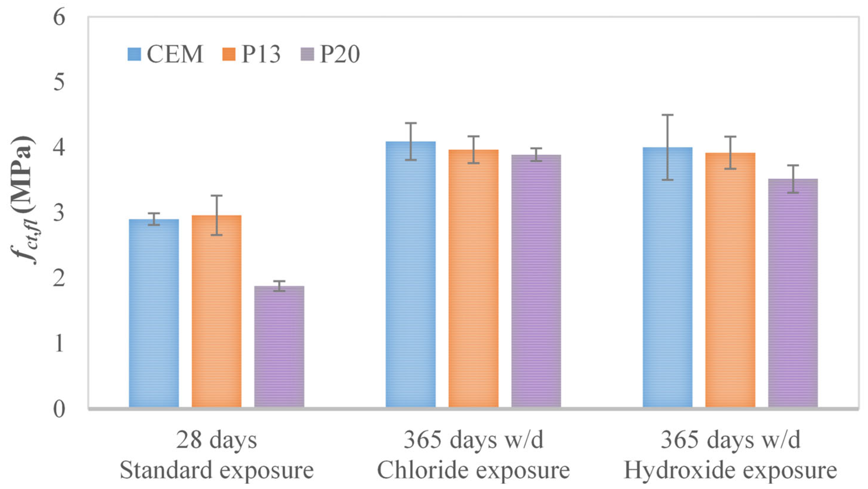
| Mix | fct,fl,28 (MPa) | fct,fl,365,Cl (MPa) | fct,fl,365,hydro (MPa) |
|---|---|---|---|
| CEM | 2.90 ± 0.09 | 4.09 ± 0.28 | 4.00 ± 0.50 |
| P13 | 2.96 ± 0.30 | 3.97 ± 0.21 | 3.92 ± 0.25 |
| P20 | 1.88 ± 0.08 | 3.89 ± 0.10 | 3.52 ± 0.21 |
| Mix | Gf,28 (N/m) | Gf,365,Cl (N/m) | Gf,365,hydro (N/m) |
|---|---|---|---|
| CEM | 84.7 ± 16.3 | 99.4 ± 10.2 | 103.9 ± 10.3 |
| P13 | 109.9 ± 8.6 | 129.9 ± 16.5 | 122.8 ± 5.8 |
| P20 | 165.5 ± 14.6 | 179.4 ± 14.5 | 203.2 ± 37.4 |
| Time: w/d Cycles | 4 | 8 | 12 | 19 | 26 |
|---|---|---|---|---|---|
| Ecor/VSCE | −0.129 | −0.158 | −0.263 | −0.315 | −0.373 |
| Rs+m/Ω cm2 | 346 | 507 | 391 | 379 | 465 |
| Rf/Ω cm2 | 68 | 60 | 60 | 110 | 95 |
| Cf/µF cm−2 | 154 | 74 | 39 | 98 | 166 |
| Rct/kΩ cm2 | 1360 | 6129 | 888 | 253 | 38 |
| Cdl/µF cm−2 | 273 | 253 | 244 | 234 | 270 |
| Time: w/d Cycles | 4 | 8 | 12 | 19 | 26 |
|---|---|---|---|---|---|
| Ecor/VSCE | −0.187 | −0.174 | −0.158 | −0.178 | −0.273 |
| Rs+m/Ω cm2 | 525 | 475 | 520 | 488 | 687 |
| Rf/Ω cm2 | 66 | 70 | 98 | 100 | 122 |
| Cf/µF cm−2 | 185 | 129 | 53 | 102 | 40 |
| Rct/kΩ cm2 | 3086 | 5817 | 7962 | 2946 | 235 |
| Cdl/µF cm−2 | 274 | 271 | 270 | 239 | 222 |
Disclaimer/Publisher’s Note: The statements, opinions and data contained in all publications are solely those of the individual author(s) and contributor(s) and not of MDPI and/or the editor(s). MDPI and/or the editor(s) disclaim responsibility for any injury to people or property resulting from any ideas, methods, instructions or products referred to in the content. |
© 2025 by the authors. Licensee MDPI, Basel, Switzerland. This article is an open access article distributed under the terms and conditions of the Creative Commons Attribution (CC BY) license (https://creativecommons.org/licenses/by/4.0/).
Share and Cite
Zanotto, F.; Sirico, A.; Balbo, A.; Bernardi, P.; Merchiori, S.; Grassi, V.; Belletti, B.; Monticelli, C. Experimental Investigation of Steel Bar Corrosion in Recycled Plastic Aggregate Concrete Exposed to Calcium Chloride Cycles. Materials 2025, 18, 3361. https://doi.org/10.3390/ma18143361
Zanotto F, Sirico A, Balbo A, Bernardi P, Merchiori S, Grassi V, Belletti B, Monticelli C. Experimental Investigation of Steel Bar Corrosion in Recycled Plastic Aggregate Concrete Exposed to Calcium Chloride Cycles. Materials. 2025; 18(14):3361. https://doi.org/10.3390/ma18143361
Chicago/Turabian StyleZanotto, Federica, Alice Sirico, Andrea Balbo, Patrizia Bernardi, Sebastiano Merchiori, Vincenzo Grassi, Beatrice Belletti, and Cecilia Monticelli. 2025. "Experimental Investigation of Steel Bar Corrosion in Recycled Plastic Aggregate Concrete Exposed to Calcium Chloride Cycles" Materials 18, no. 14: 3361. https://doi.org/10.3390/ma18143361
APA StyleZanotto, F., Sirico, A., Balbo, A., Bernardi, P., Merchiori, S., Grassi, V., Belletti, B., & Monticelli, C. (2025). Experimental Investigation of Steel Bar Corrosion in Recycled Plastic Aggregate Concrete Exposed to Calcium Chloride Cycles. Materials, 18(14), 3361. https://doi.org/10.3390/ma18143361