
Determining the Shear Capacity of Steel Beams with Corrugated Webs by Using Optimised Regression Learner Techniques


Abstract
:1. Introduction
2. Theoretical Background
3. Assessment of SBCW Shear Capacity Formulas
4. Test Data
4.1. Test Data Published by Other Researchers
4.2. Test Data from the Authors
4.3. Test Setup
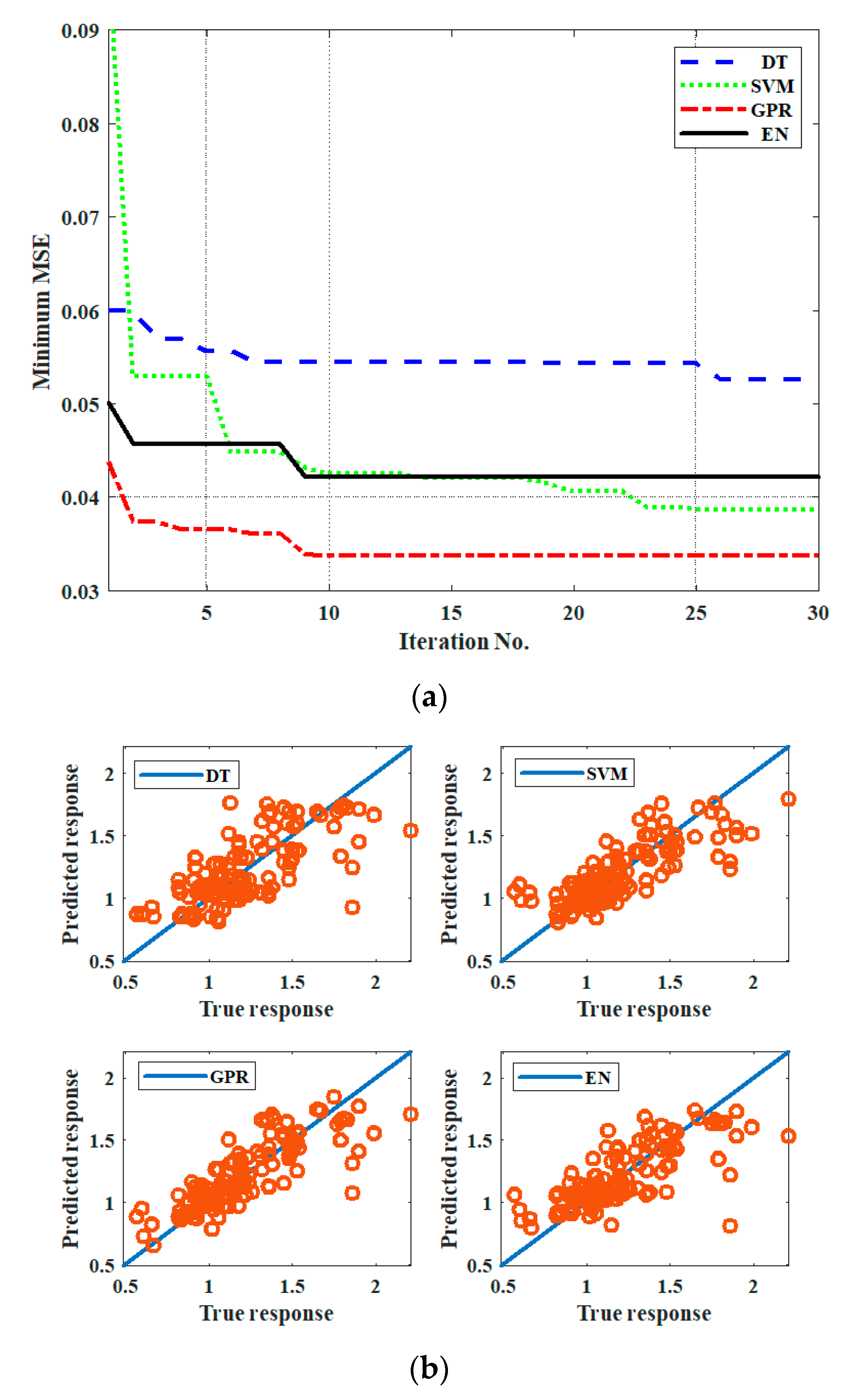
5. ORLTs
- The validation technique was selected, the cross-validation technique with 10 folds was chosen before the training process.
- The primary optimisation options were selected, and the option used was the BO technique, with an expected improvement per second plus and 30 iterations.
- One of the ORLTs was selected (DT, SVM, GPR or EN).
- The training process is started to determine the optimal parameters and predicted model of this method.
- The optimal parameters and performance model of the selected method were recorded.
- Finally, the ORLT model of the selected method was exported to be used in the prediction of the original and new datasets.
6. Model Validation and Comparison
7. Initial Comparison with Published Experimental Data
8. Conclusions
Author Contributions
Funding
Institutional Review Board Statement
Informed Consent Statement
Data Availability Statement
Acknowledgments
Conflicts of Interest
Appendix A. Experimental Data

| Specimen ID | hw | a | tw | Corrugation Dimensions | Fyw | Web Slenderness | ||
|---|---|---|---|---|---|---|---|---|
| b | hr | d | ||||||
| L1A | 994 | 974 | 2 | 140 | 50.03 | 50 | 292 | 512.37 |
| L1B | 994 | 984 | 3 | 140 | 50.03 | 50 | 335 | 383.78 |
| L2A | 1445 | 1503 | 2 | 140 | 50.03 | 50 | 282 | 744.85 |
| L2B | 1445 | 1503 | 3 | 140 | 50.03 | 50 | 317 | 568.90 |
| L3A | 2005 | 2005 | 2 | 140 | 50.03 | 50 | 280 | 997.51 |
| L3B | 2005 | 2005 | 3 | 140 | 50.03 | 50 | 300 | 792.49 |
| B1 | 600 | 798 | 2 | 140 | 50.03 | 50 | 341 | 285.71 |
| B4 | 600 | 798 | 2 | 140 | 50.03 | 50 | 363 | 284.36 |
| B4b | 600 | 798 | 2 | 140 | 50.03 | 50 | 363 | 284.36 |
| B3 | 600 | 798 | 3 | 140 | 50.03 | 50 | 317 | 229.01 |
| B2 | 600 | 702 | 3 | 140 | 50.03 | 50 | 315 | 229.01 |
| M101 | 600 | 600 | 1 | 70 | 15.01 | 15 | 189 | 606.06 |
| M102 | 800 | 800 | 1 | 70 | 15.01 | 15 | 190 | 808.08 |
| M103 | 1000 | 1000 | 1 | 70 | 15.01 | 15 | 213 | 1052.63 |
| M104 | 1200 | 1200 | 1 | 70 | 15.01 | 15 | 189 | 1212.12 |
| L1 | 1000 | 1500 | 2 | 106 | 50.02 | 87 | 410 | 476.19 |
| L1 | 1000 | 1490 | 3 | 106 | 50.02 | 87 | 450 | 333.33 |
| L2 | 1498 | 2157 | 2 | 106 | 50.02 | 87 | 376 | 749.00 |
| L2 | 1498 | 2142 | 3 | 106 | 50.02 | 87 | 402 | 499.33 |
| No. 1 | 850 | 1131 | 2 | 102 | 55.55 | 86 | 355 | 425.00 |
| No. 2 | 850 | 1131 | 2 | 91 | 56.30 | 72 | 349 | 425.00 |
| V1/1 | 298 | 2819 | 2 | 144 | 102.06 | 102 | 298 | 145.37 |
| V1/2 | 298 | 2000 | 2 | 144 | 102.06 | 102 | 283 | 141.90 |
| V1/3 | 298 | 1001 | 2 | 144 | 102.06 | 102 | 298 | 149.00 |
| V2/3 | 600 | 1650 | 3 | 144 | 102.06 | 102 | 279 | 200.00 |
| Specimen ID | hw | a | tw | Corrugation Dimensions | Fyw | Web Slenderness | ||
|---|---|---|---|---|---|---|---|---|
| b | hr | d | ||||||
| V-PILOTA | 305 | 305 | 0.78 | 38.10 | 25.42 | 25.40 | 621 | 390.03 |
| V-PILOTB | 305 | 305 | 0.79 | 38.10 | 25.42 | 25.40 | 638 | 388.54 |
| V121216A | 305 | 305 | 0.64 | 38.10 | 25.42 | 25.40 | 676 | 478.06 |
| V121216B | 305 | 305 | 0.77 | 38.10 | 25.42 | 25.40 | 665 | 398.69 |
| V181216B | 457 | 305 | 0.61 | 38.10 | 25.42 | 25.40 | 618 | 749.18 |
| V181216C | 457 | 305 | 0.76 | 38.10 | 25.42 | 25.40 | 679 | 602.11 |
| V181816A | 457 | 457 | 0.64 | 38.10 | 25.42 | 25.40 | 591 | 719.69 |
| V181816B | 457 | 457 | 0.74 | 38.10 | 25.42 | 25.40 | 614 | 620.08 |
| V241216A | 610 | 305 | 0.64 | 38.10 | 25.42 | 25.40 | 591 | 960.63 |
| V241216B | 610 | 305 | 0.79 | 38.10 | 25.42 | 25.40 | 588 | 775.10 |
| V121221A | 305 | 305 | 0.63 | 41.90 | 33.45 | 23.40 | 665 | 484.13 |
| V121221B | 305 | 305.00 | 0.79 | 41.90 | 33.45 | 23.40 | 665 | 388.54 |
| V122421A | 305 | 609.60 | 0.68 | 41.90 | 33.45 | 23.40 | 621 | 451.18 |
| V122421B | 305 | 609.60 | 0.78 | 41.90 | 33.45 | 23.40 | 638 | 390.03 |
| V181221A | 457 | 305 | 0.61 | 41.90 | 33.45 | 23.40 | 578 | 749.18 |
| V181221B | 457 | 305 | 0.76 | 41.90 | 33.45 | 23.40 | 606 | 599.74 |
| V181821A | 457 | 457 | 0.64 | 41.90 | 33.45 | 23.40 | 552 | 719.69 |
| V181821B | 457 | 457 | 0.74 | 41.90 | 33.45 | 23.40 | 596 | 620.08 |
| V241221A | 610 | 305 | 0.61 | 41.90 | 33.45 | 23.40 | 610 | 1000.00 |
| V241221B | 610 | 305 | 0.76 | 41.90 | 33.45 | 23.40 | 639 | 800.52 |
| V121232A | 305 | 305 | 0.64 | 49.80 | 50.77 | 26.40 | 665 | 476.56 |
| V121232B | 305 | 305 | 0.78 | 49.80 | 50.77 | 26.40 | 641 | 391.03 |
| V121832A | 305 | 457 | 0.64 | 49.80 | 50.77 | 26.40 | 703 | 476.56 |
| V121832B | 305 | 457 | 0.92 | 49.80 | 50.77 | 26.40 | 562 | 331.88 |
| V122432A | 305 | 609.60 | 0.64 | 49.80 | 50.77 | 26.40 | 714 | 476.56 |
| V122432B | 305 | 609.60 | 0.78 | 49.80 | 50.77 | 26.40 | 634 | 392.54 |
| V181232A | 457 | 305 | 0.60 | 49.80 | 50.77 | 26.40 | 552 | 765.49 |
| V181232B | 457 | 305 | 0.75 | 49.80 | 50.77 | 26.40 | 602 | 610.15 |
| V181832A | 457 | 457 | 0.61 | 49.80 | 50.77 | 26.40 | 689 | 749.18 |
| V181832B | 457 | 457 | 0.75 | 49.80 | 50.77 | 26.40 | 580 | 610.15 |
| V241232A | 610 | 305.00 | 0.62 | 49.80 | 50.77 | 26.40 | 673 | 980.71 |
| V241232B | 610 | 305.00 | 0.76 | 49.80 | 50.77 | 26.40 | 584 | 800.52 |
| V121809A | 305 | 457.00 | 0.71 | 19.80 | 14.19 | 11.90 | 572 | 432.01 |
| V121809C | 305 | 457.00 | 0.63 | 19.80 | 14.19 | 11.90 | 669 | 482.59 |
| V122409A | 305 | 609.60 | 0.71 | 19.80 | 14.19 | 11.90 | 586 | 427.17 |
| V122409C | 305 | 609.60 | 0.66 | 19.80 | 14.19 | 11.90 | 621 | 460.03 |
| V181209A | 457 | 305.00 | 0.56 | 19.80 | 14.19 | 11.90 | 689 | 817.53 |
| V181209C | 457 | 305.00 | 0.61 | 19.80 | 14.19 | 11.90 | 592 | 749.18 |
| V181809A | 457 | 457.00 | 0.61 | 19.80 | 14.19 | 11.90 | 618 | 749.18 |
| V181809C | 457 | 457.00 | 0.62 | 19.80 | 14.19 | 11.90 | 559 | 734.73 |
| V241209A | 610 | 305.00 | 0.62 | 19.80 | 14.19 | 11.90 | 606 | 980.71 |
| V241209C | 610 | 305.00 | 0.64 | 19.80 | 14.19 | 11.90 | 621 | 960.63 |
| Specimen ID | hw | a | tw | Corrugation Dimensions | Fyw | Web Slenderness | ||
|---|---|---|---|---|---|---|---|---|
| b | hr | d | ||||||
| CW1 | 440.36 | 730.92 | 3.06 | 180 | 45.01 | 44.99 | 320 | 143.91 |
| CW2 | 437.92 | 730.92 | 3.29 | 180 | 45.01 | 44.99 | 312 | 133.11 |
| CW3 | 437.18 | 940.92 | 3.26 | 250 | 45.01 | 44.99 | 284 | 134.10 |
| Specimen ID | hw | a | tw | Corrugation Dimensions | Fyw | Web Slenderness | ||
|---|---|---|---|---|---|---|---|---|
| b | hr | d | ||||||
| SP1 | 800 | 1750 | 2 | 146 | 104.07 | 104 | 307 | 400 |
| SP2 | 800 | 1750 | 2 | 170 | 80.05 | 80 | 299 | 400 |
| SP3 | 800 | 1750 | 2 | 185 | 65.04 | 65 | 292 | 400 |
| SP4 | 800 | 1800 | 2 | 117 | 83.05 | 83 | 298 | 400 |
| SP5 | 800 | 1800 | 2 | 136 | 64.04 | 64 | 291 | 400 |
| SP6 | 800 | 1800 | 2 | 148 | 52.03 | 52 | 294 | 400 |
| SP2-2-400 1 | 400 | 1000 | 2 | 170 | 80.05 | 80 | 263 | 200 |
| SP2-2-400 2 | 400 | 1000 | 2 | 170 | 80.05 | 80 | 263 | 200 |
| SP2-2-800 1 | 800 | 1000 | 2 | 170 | 80.05 | 80 | 272 | 400 |
| SP2-2-800 2 | 800 | 1000 | 2 | 170 | 80.05 | 80 | 272 | 400 |
| SP2-3-600 1 | 600 | 1000 | 3 | 170 | 80.05 | 80 | 294 | 200 |
| SP2-3-600 2 | 600 | 1000 | 3 | 170 | 80.05 | 80 | 294 | 200 |
| SP2-3-1200 1 | 1200 | 1000 | 3 | 170 | 80.05 | 80 | 294 | 400 |
| SP2-3-1200 2 | 1200 | 1000 | 3 | 170 | 80.05 | 80 | 294 | 400 |
| SP2-4-800 1 | 800 | 1000 | 4 | 170 | 80.05 | 80 | 326 | 200 |
| SP2-4-800 2 | 800 | 1000 | 4 | 170 | 80.05 | 80 | 326 | 200 |
| SP2-4-1600 1 | 1600 | 1000 | 4 | 170 | 80.05 | 80 | 328 | 400 |
| SP2-4-1600 2 | 1600 | 1000 | 4 | 170 | 80.05 | 80 | 328 | 400 |
| SP2-8-800 1 | 800 | 1000 | 8 | 170 | 80.05 | 80 | 270 | 100 |
| SP2-8-800 2 | 800 | 1000 | 8 | 170 | 80.05 | 80 | 270 | 100 |
| Specimen ID | hw | a | tw | Corrugation Dimensions | Fyw | Web Slenderness | ||
|---|---|---|---|---|---|---|---|---|
| b | hr | d | ||||||
| G7A | 1500 | 4500 | 6 | 300 | 150 | 200 | 465 | 250 |
| G8A | 1500 | 4500 | 6 | 300 | 150 | 200 | 465 | 250 |
| Specimen ID | hw | a | tw | Corrugation Dimensions | Fyw | Web Slenderness | ||
|---|---|---|---|---|---|---|---|---|
| b | hr | d | ||||||
| L1 | 1500 | 3000 | 4.80 | 450 | 200.00 | 300 | 250 | 312.50 |
| L2 | 1500 | 3400 | 4.80 | 550 | 188.80 | 300 | 250 | 312.50 |
| L3 | 1500 | 3000 | 4.80 | 450 | 49.60 | 300 | 250 | 312.50 |
| L4 | 1500 | 3400 | 4.80 | 550 | 55.60 | 300 | 250 | 312.50 |
| I1 | 2000 | 3600 | 4.80 | 320 | 44.60 | 100 | 250 | 416.67 |
| I2 | 2000 | 3600 | 3.80 | 350 | 28.60 | 100 | 250 | 526.32 |
| G1 | 2000 | 3000 | 4.80 | 200 | 45.40 | 180 | 250 | 416.67 |
| G2 | 2000 | 3000 | 3.80 | 160 | 33.00 | 50 | 250 | 526.32 |
| G3 | 2000 | 3000 | 3.80 | 160 | 26.90 | 100 | 250 | 526.32 |
| Specimen ID | hw | a | tw | Corrugation Dimensions | Fyw | Web Slenderness | ||
|---|---|---|---|---|---|---|---|---|
| b | hr | d | ||||||
| PG2 | 2000 | 2600 | 4 | 250 | 60 | 220 | 296 | 500 |
| PG1 | 2000 | 2800 | 4 | 220 | 60 | 180 | 296 | 500 |
| PG3 | 2000 | 2800 | 4 | 220 | 75 | 180 | 296 | 500 |
| Specimen ID | hw | a | tw | Corrugation Dimensions | Fyw | Web Slenderness | ||
|---|---|---|---|---|---|---|---|---|
| b | hr | d | ||||||
| TP20-300-30 | 3050 | 664.90 | 2 | 60 | 20.01 | 34.64 | 290 | 152.50 |
| A20-410-30-N | 410 | 578.10 | 2 | 40 | 20.01 | 34.64 | 290 | 205.00 |
| A20-410-45-N | 410 | 524.80 | 2 | 40 | 28.29 | 28.28 | 290 | 205.00 |
| A20-505-30-N | 505 | 575.70 | 2 | 40 | 20.01 | 34.64 | 290 | 252.50 |
| A20-505-45-N | 505 | 525.20 | 2 | 40 | 28.29 | 28.28 | 290 | 252.50 |
| B20-305-30 | 305 | 427.00 | 2 | 40 | 20.01 | 34.64 | 680 | 152.50 |
| B20-305-45 | 305 | 390.40 | 2 | 40 | 28.29 | 28.28 | 680 | 152.50 |
| B20-505-45 | 505 | 388.85 | 2 | 40 | 28.29 | 28.28 | 680 | 252.50 |
| B20-505-45-N | 505 | 388.85 | 2 | 40 | 28.29 | 28.28 | 290 | 252.50 |
| Specimen ID | hw | a | tw | Corrugation Dimensions | Fyw | Web Slenderness | ||
|---|---|---|---|---|---|---|---|---|
| b | hr | d | ||||||
| W1 | 1200 | 2000 | 3 | 110 | 55 | 90 | 400 | 400 |
| SC1 | 1500 | 4500 | 6.27 | 300 | 150 | 200 | 465 | 239.23 |
| V1b | 500 | 1000 | 2.50 | 30 | 40 | 47 | 270 | 200 |
| Specimen ID | λL | λG | λI,1 | ρ e | ζ | V (kN) | VT (kN) | V/VT |
|---|---|---|---|---|---|---|---|---|
| L1A | 0.953 | 0.53 | 1.09 | 0.70 | 1.255 | 281.72 | 280.93 | 1.01 |
| L1B | 0.765 | 0.53 | 0.93 | 0.80 | 1.238 | 495.08 | 501.34 | 0.98 |
| L2A | 0.937 | 0.76 | 1.21 | 0.63 | 1.222 | 347.69 | 337.50 | 1.04 |
| L2B | 0.759 | 0.75 | 1.07 | 0.71 | 1.182 | 571.69 | 563.51 | 1.00 |
| L3A | 0.901 | 1.04 | 1.38 | 0.52 | 1.384 | 465.59 | 451.22 | 1.05 |
| L3B | 0.741 | 1.02 | 1.26 | 0.60 | 1.460 | 776.65 | 773.57 | 0.99 |
| B1 | 0.952 | 0.34 | 1.01 | 0.75 | 1.056 | 202.53 | 208.04 | 0.94 |
| B4 | 0.977 | 0.35 | 1.04 | 0.73 | 1.062 | 203.28 | 183.46 | 1.12 |
| B4b | 0.977 | 0.35 | 1.04 | 0.73 | 1.062 | 203.28 | 217.66 | 0.95 |
| B3 | 0.735 | 0.31 | 0.80 | 0.88 | 1.008 | 255.36 | 246.01 | 1.04 |
| B2 | 0.733 | 0.31 | 0.80 | 0.88 | 1.061 | 263.45 | 273.42 | 0.98 |
| M101 | 0.751 | 0.74 | 1.05 | 0.72 | 1.153 | 53.46 | 52.96 | 1.02 |
| M102 | 0.753 | 0.99 | 1.24 | 0.60 | 1.507 | 79.10 | 79.19 | 1.00 |
| M103 | 0.831 | 1.32 | 1.56 | 0.41 | 1.751 | 83.79 | 83.95 | 1.00 |
| M104 | 0.751 | 1.48 | 1.66 | 0.36 | 2.168 | 102.33 | 103.98 | 0.98 |
| L1 | 0.790 | 0.66 | 1.03 | 0.74 | 1.045 | 383.35 | 380.08 | 1.01 |
| L1 | 0.579 | 0.63 | 0.86 | 0.84 | 0.945 | 617.09 | 610.72 | 1.01 |
| L2 | 0.794 | 0.96 | 1.25 | 0.60 | 1.506 | 592.39 | 600.20 | 0.98 |
| L2 | 0.548 | 0.90 | 1.05 | 0.72 | 1.202 | 899.87 | 905.32 | 1.00 |
| No. 1 | 0.743 | 0.48 | 0.88 | 0.83 | 0.948 | 272.59 | 275.01 | 0.99 |
| No. 2 | 0.657 | 0.47 | 0.81 | 0.87 | 0.918 | 272.46 | 264.27 | 1.04 |
| V1/1 | 0.939 | 0.10 | 0.94 | 0.79 | 0.820 | 67.96 | 67.98 | 1.00 |
| V1/2 | 0.894 | 0.09 | 0.90 | 0.82 | 0.837 | 69.87 | 69.84 | 1.00 |
| V1/3 | 0.963 | 0.10 | 0.97 | 0.77 | 0.992 | 79.08 | 80.93 | 0.97 |
| V2/3 | 0.621 | 0.17 | 0.64 | 0.97 | 0.844 | 236.78 | 234.89 | 1.01 |
| Specimen ID | λL | λG | λI,1 | ρ e | ζ | V (kN) | VT (kN) | V/VT |
|---|---|---|---|---|---|---|---|---|
| V-PILOTA | 0.939 | 0.52 | 1.07 | 0.71 | 1.284 | 76.65 | 82.73 | 0.94 |
| V-PILOTB | 0.948 | 0.52 | 1.08 | 0.70 | 1.290 | 78.78 | 71.17 | 1.12 |
| V121216A | 1.200 | 0.57 | 1.33 | 0.55 | 1.249 | 50.51 | 50.05 | 1.05 |
| V121216B | 0.993 | 0.54 | 1.13 | 0.67 | 1.300 | 80.36 | 87.63 | 0.90 |
| V181216B | 1.200 | 0.82 | 1.46 | 0.47 | 1.870 | 89.05 | 93.41 | 0.94 |
| V181216C | 1.011 | 0.82 | 1.30 | 0.57 | 1.537 | 117.97 | 119.47 | 1.00 |
| V181816A | 1.128 | 0.80 | 1.38 | 0.52 | 1.492 | 75.66 | 74.73 | 1.03 |
| V181816B | 0.990 | 0.78 | 1.26 | 0.59 | 1.370 | 96.48 | 96.17 | 1.01 |
| V241216A | 1.128 | 1.06 | 1.55 | 0.42 | 1.423 | 77.15 | 75.57 | 1.04 |
| V241216B | 0.908 | 1.01 | 1.35 | 0.54 | 1.494 | 133.19 | 133.35 | 0.98 |
| V121221A | 1.326 | 0.45 | 1.40 | 0.51 | 1.238 | 47.01 | 46.26 | 1.01 |
| V121221B | 1.064 | 0.42 | 1.15 | 0.67 | 1.188 | 75.75 | 72.50 | 1.00 |
| V122421A | 1.194 | 0.42 | 1.27 | 0.59 | 1.034 | 44.47 | 43.28 | 1.04 |
| V122421B | 1.046 | 0.41 | 1.13 | 0.68 | 1.017 | 61.61 | 61.20 | 0.99 |
| V181221A | 1.277 | 0.63 | 1.42 | 0.49 | 1.380 | 64.04 | 61.83 | 1.02 |
| V181221B | 1.046 | 0.61 | 1.21 | 0.62 | 1.301 | 99.89 | 97.86 | 1.01 |
| V181821A | 1.198 | 0.61 | 1.34 | 0.54 | 1.208 | 58.44 | 56.49 | 1.07 |
| V181821B | 1.073 | 0.61 | 1.23 | 0.61 | 1.269 | 92.84 | 93.41 | 0.96 |
| V241221A | 1.312 | 0.86 | 1.57 | 0.41 | 1.481 | 78.46 | 77.26 | 1.02 |
| V241221B | 1.075 | 0.84 | 1.36 | 0.53 | 1.403 | 130.66 | 126.72 | 1.01 |
| V121232A | 1.782 | 0.30 | 1.81 | 0.31 | 1.702 | 39.58 | 41.14 | 0.95 |
| V121232B | 1.436 | 0.28 | 1.46 | 0.47 | 1.460 | 59.92 | 61.16 | 0.98 |
| V121832A | 1.833 | 0.31 | 1.86 | 0.29 | 1.493 | 34.40 | 34.47 | 0.99 |
| V121832B | 1.141 | 0.25 | 1.17 | 0.65 | 0.994 | 54.68 | 53.38 | 1.10 |
| V122432A | 1.847 | 0.31 | 1.87 | 0.28 | 1.360 | 31.35 | 31.14 | 1.00 |
| V122432B | 1.434 | 0.28 | 1.46 | 0.47 | 1.175 | 49.14 | 48.93 | 0.98 |
| V181232A | 1.741 | 0.42 | 1.79 | 0.31 | 1.848 | 49.76 | 51.60 | 0.97 |
| V181232B | 1.449 | 0.41 | 1.51 | 0.44 | 1.536 | 79.59 | 80.06 | 1.00 |
| V181832A | 1.904 | 0.47 | 1.96 | 0.26 | 1.810 | 52.07 | 52.93 | 0.99 |
| V181832B | 0.939 | 0.52 | 1.07 | 0.71 | 1.284 | 76.65 | 82.73 | 0.94 |
| V241232A | 1.422 | 0.41 | 1.48 | 0.46 | 1.505 | 78.12 | 78.64 | 1.00 |
| V241232B | 1.845 | 0.61 | 1.94 | 0.26 | 1.765 | 69.16 | 69.08 | 1.00 |
| V121809A | 1.403 | 0.54 | 1.50 | 0.44 | 1.485 | 103.31 | 101.46 | 1.01 |
| V121809C | 0.519 | 0.78 | 0.94 | 0.79 | 1.070 | 62.39 | 63.16 | 0.95 |
| V122409A | 0.626 | 0.87 | 1.07 | 0.71 | 1.101 | 56.55 | 55.16 | 1.05 |
| V122409C | 0.519 | 0.79 | 0.95 | 0.79 | 1.026 | 59.74 | 57.82 | 1.03 |
| V181209A | 0.575 | 0.83 | 1.01 | 0.75 | 1.061 | 57.65 | 57.82 | 1.00 |
| V181209C | 0.719 | 1.37 | 1.54 | 0.42 | 1.880 | 79.95 | 80.95 | 0.99 |
| V181809A | 0.611 | 1.24 | 1.38 | 0.52 | 1.766 | 87.08 | 88.78 | 0.99 |
| V181809C | 0.624 | 1.27 | 1.41 | 0.50 | 1.626 | 83.94 | 82.29 | 0.99 |
| V241209A | 0.582 | 1.20 | 1.33 | 0.55 | 1.584 | 77.56 | 77.62 | 1.03 |
| V241209C | 0.606 | 1.67 | 1.77 | 0.32 | 1.737 | 71.90 | 70.77 | 1.04 |
| Specimen ID | λL | λG | λI,1 | ρ e | ζ | V (kN) | VT (kN) | V/VT |
|---|---|---|---|---|---|---|---|---|
| CW1 | 0.813 | 0.34 | 0.88 | 0.83 | 0.660 | 133.74 | 126.59 | 1.07 |
| CW2 | 0.747 | 0.33 | 0.82 | 0.87 | 0.669 | 152.26 | 150.56 | 1.00 |
| CW3 | 0.999 | 0.35 | 1.06 | 0.72 | 0.667 | 110.05 | 100.22 | 1.12 |
| Specimen ID | λL | λG | λI,1 | ρ e | ζ | V (kN) | VT (kN) | V/VT |
|---|---|---|---|---|---|---|---|---|
| SP1 | 0.996 | 0.26 | 1.03 | 0.74 | 1.077 | 224.99 | 225.00 | 1.00 |
| SP2 | 1.136 | 0.35 | 1.19 | 0.64 | 1.202 | 213.74 | 215.30 | 0.98 |
| SP3 | 1.222 | 0.44 | 1.30 | 0.57 | 1.324 | 205.69 | 209.50 | 0.97 |
| SP4 | 0.783 | 0.30 | 0.84 | 0.85 | 0.999 | 232.31 | 230.80 | 1.02 |
| SP5 | 0.897 | 0.41 | 0.99 | 0.76 | 1.095 | 222.07 | 220.50 | 1.02 |
| SP6 | 0.981 | 0.53 | 1.11 | 0.68 | 1.177 | 218.68 | 220.00 | 0.99 |
| SP2-2-400 1 | 1.066 | 0.16 | 1.08 | 0.71 | 0.981 | 84.29 | 80.25 | 1.05 |
| SP2-2-400 2 | 1.066 | 0.16 | 1.08 | 0.71 | 0.981 | 84.29 | 88.13 | 0.95 |
| SP2-2-800 1 | 1.084 | 0.33 | 1.13 | 0.67 | 1.060 | 178.87 | 178.88 | 1.00 |
| SP2-2-800 2 | 1.084 | 0.33 | 1.13 | 0.67 | 1.060 | 178.87 | 177.75 | 1.01 |
| SP2-3-600 1 | 0.751 | 0.24 | 0.79 | 0.89 | 1.121 | 302.98 | 301.50 | 1.00 |
| SP2-3-600 2 | 0.751 | 0.24 | 0.79 | 0.89 | 1.121 | 302.98 | 308.63 | 0.98 |
| SP2-3-1200 1 | 0.751 | 0.47 | 0.89 | 0.82 | 1.221 | 614.51 | 611.25 | 1.01 |
| SP2-3-1200 2 | 0.751 | 0.47 | 0.89 | 0.82 | 1.221 | 614.51 | 625.13 | 0.98 |
| SP2-4-800 1 | 0.593 | 0.31 | 0.67 | 0.96 | 1.056 | 603.28 | 601.50 | 1.01 |
| SP2-4-800 2 | 0.593 | 0.31 | 0.67 | 0.96 | 1.056 | 603.28 | 603.38 | 1.01 |
| SP2-4-1600 1 | 0.595 | 0.62 | 0.86 | 0.84 | 1.197 | 1218.89 | 1215.38 | 1.00 |
| SP2-4-1600 2 | 0.595 | 0.62 | 0.86 | 0.84 | 1.197 | 1218.89 | 1227.00 | 0.99 |
| SP2-8-800 1 | 0.270 | 0.24 | 0.36 | 1.00 | 1.330 | 1332.58 | 1308.38 | 1.01 |
| SP2-8-800 2 | 0.270 | 0.24 | 0.36 | 1.00 | 1.330 | 1332.58 | 1374.75 | 0.97 |
| Specimen ID | λL | λG | λI,1 | ρ e | ζ | V (kN) | VT (kN) | V/VT |
|---|---|---|---|---|---|---|---|---|
| G7A | 0.834 | 0.37 | 0.91 | 0.81 | 1.084 | 2190.70 | 2299.82 | 0.92 |
| G8A | 0.834 | 0.37 | 0.91 | 0.81 | 1.084 | 2190.70 | 2155.05 | 0.98 |
| Specimen ID | λL | λG | λI,1 | ρ e | ζ | V (kN) | VT (kN) | V/VT |
|---|---|---|---|---|---|---|---|---|
| L1 | 1.146 | 0.22 | 1.17 | 0.65 | 1.097 | 743.50 | 745.62 | 1.00 |
| L2 | 1.401 | 0.23 | 1.42 | 0.50 | 1.209 | 624.38 | 625.56 | 1.00 |
| L3 | 1.146 | 0.63 | 1.31 | 0.57 | 0.921 | 540.06 | 532.02 | 1.02 |
| L4 | 1.401 | 0.56 | 1.51 | 0.44 | 1.052 | 480.55 | 474.73 | 1.01 |
| I1 | 0.815 | 0.86 | 1.18 | 0.64 | 1.463 | 1302.50 | 1313.50 | 0.99 |
| I2 | 1.126 | 1.26 | 1.69 | 0.35 | 1.475 | 565.15 | 565.66 | 1.00 |
| G1 | 0.509 | 0.91 | 1.04 | 0.73 | 1.077 | 1087.70 | 1095.96 | 0.99 |
| G2 | 0.515 | 1.14 | 1.25 | 0.60 | 1.392 | 916.69 | 912.94 | 1.01 |
| G3 | 0.515 | 1.39 | 1.48 | 0.46 | 1.759 | 888.05 | 929.62 | 0.94 |
| Specimen ID | λL | λG | λI,1 | ρ e | ζ | V (kN) | VT (kN) | V/VT |
|---|---|---|---|---|---|---|---|---|
| PG2 | 0.831 | 0.85 | 1.19 | 0.64 | 0.998 | 869.56 | 873.60 | 0.99 |
| PG1 | 0.732 | 0.87 | 1.13 | 0.67 | 0.946 | 864.75 | 843.20 | 1.03 |
| PG3 | 0.732 | 0.73 | 1.03 | 0.74 | 1.053 | 1052.21 | 1052.80 | 1.01 |
| Specimen ID | λL | λG | λI,1 | ρ e | ζ | V (kN) | VT (kN) | V/VT |
|---|---|---|---|---|---|---|---|---|
| TP20-300-30 | 0.395 | 0.38 | 0.55 | 1.00 | 0.833 | 84.89 | 84.72 | 1.00 |
| A20-410-30-N | 0.263 | 0.45 | 0.52 | 1.00 | 0.899 | 122.74 | 125.09 | 0.99 |
| A20-410-45-N | 0.263 | 0.34 | 0.43 | 1.00 | 0.857 | 118.28 | 116.46 | 1.01 |
| A20-505-30-N | 0.263 | 0.56 | 0.62 | 0.99 | 0.915 | 153.69 | 154.23 | 0.99 |
| A20-505-45-N | 0.263 | 0.42 | 0.50 | 1.00 | 0.895 | 152.72 | 152.49 | 0.99 |
| B20-305-30 | 0.403 | 0.51 | 0.65 | 0.97 | 1.006 | 233.51 | 233.20 | 1.00 |
| B20-305-45 | 0.403 | 0.39 | 0.56 | 1.00 | 1.044 | 248.99 | 251.72 | 0.99 |
| B20-505-45 | 0.403 | 0.64 | 0.76 | 0.90 | 0.976 | 335.82 | 329.34 | 1.06 |
| B20-505-45-N | 0.263 | 0.42 | 0.50 | 1.00 | 0.852 | 150.59 | 150.43 | 0.96 |
References
- Lindner, J.; Aschinger, R. Grenzschubtragfähigkeit von I-trägern mit trapezför- mig profilierten Stegen; Stahlbau: Aurich, Germany, 1988; Volume 57, pp. 377–380. [Google Scholar]
- Elgaaly, M.; Hamilton, R.; Seshadri, A. Shear strength of beams with corrugated webs. J. Struct. Eng. 1996, 122, 390–398. [Google Scholar] [CrossRef]
- Sause, R.; Abbas, H.; Wassef, W.; Driver, R.; Elgaaly, M. Corrugated Web Girder Shape and Strength Criteria: Work area 1. Pennsylvania Innovative High Performance Steel Bridge Demonstration Project, ATLSS Report No. 03–18; Lehigh University ATLSS Center: Bethlehem, PA, USA, 2003. [Google Scholar]
- Abbas, H. Analysis and Design of Corrugated Web I—Girders for Bridges Using High Performance Steel. Ph.D. Thesis, Department of Civil and Environmental Engineering, Lehigh University, Bethlehem, PA, USA, 2003. [Google Scholar]
- Driver, G.; Abbas, H.; Sause, R. Shear behavior of corrugated web bridge girders. J. Struct. Eng. 2006, 132, 195–203. [Google Scholar] [CrossRef]
- Yi, J.; Gil, H.; Youm, K.; Lee, H. Interactive shear buckling behavior of trapezoidally corrugated steel webs. Eng. Struct. 2008, 30, 1659–1666. [Google Scholar] [CrossRef]
- Moon, J.; Yi, J.; Choi, H.; Lee, H.-E. Shear strength and design of trapezoidally corrugated steel webs. J. Constr. Steel Res. 2008, 65, 1198–1205. [Google Scholar] [CrossRef]
- Sause, R.; Braxtan, T. Shear strength of trapezoidal corrugated steel webs. J. Constr. Steel Res. 2011, 67, 223–236. [Google Scholar] [CrossRef]
- Bergfelt, A.; Leiva, L. Shear Buckling of Trapezoidally Corrugated Girders Webs, Report Part 2, Pibl.SS4:2; Sweden Chalmers University of Technology: Gothenburg, Sweden, 1984. [Google Scholar]
- El-Metwally, A. Prestressed Composite Girders with Corrugated Steel Webs. Master’s Thesis, Department of Civil Engineering, University of Calgary, Calgary, AB, Canada, 1998. [Google Scholar]
- Abbas, H.; Sause, R.; Driver, R. Shear strength and stability of high performance steel corrugated web girders. Proc. Struct. Stab. Res. Counc. 2002, 361–387. [Google Scholar]
- Hiroshi, S.; Hiroyuki, I.; Yohiaki, I.; Koichi, K. Flexural shear behavior of composite bridge girder with corrugated steel webs around middle support. Doboku Gakkai Ronbunshu 2003, 724, 49–67. [Google Scholar]
- Ahmed, S. Plate girders with corrugated steel webs. AISC Eng. J. First Quart 2005, 42, 1–13. [Google Scholar]
- Elamary, A.; Alharthi, Y.; Abdalla, O.; Alqurashi, M.; Sharaky, I. Failure mechanism of hybrid steel beams with trapezoidal corrugated-web non-welded inclined folds. Materials 2021, 14, 1424. [Google Scholar] [CrossRef] [PubMed]
- Kumar, M.; Pradeep, D.; Patel, R.; Pandian, M.; Karthikeyan, K. A study on flexural capacity of steel beams with corrugated web. Int. J. Civ. Eng. Technol. 2018, 9, 679–689. [Google Scholar]
- Krejsa, M.; Janas, P.; Čajka, R. Using DOProC method in structural reliability assessment. In Applied Mechanics and Materials; Trans Tech Publications Ltd.: Stafa-Zurich, Switzerland, 2013; pp. 300–301. [Google Scholar] [CrossRef]
- Čajka, R.; Krejsa, M. Measured data processing in civil structure using the DOProC method. In Advanced Materials Research; Trans Tech Publications Ltd.: Stafa-Zurich, Switzerland, 2013; Volume 859, pp. 114–121. [Google Scholar] [CrossRef]
- Čajka, R.; Krejsa, M. Validating a computational model of a rooflight steel structure by means of a load test. In Applied Mechanics and Materials; Trans Tech Publications Ltd.: Stafa-Zurich, Switzerland, 2014; pp. 592–598. [Google Scholar] [CrossRef]
- Flodr, J.; Krejsa, M.; Mikolášek, D.; Sucharda, O.; Žídek, I. Mathematical modelling of thin-walled cold-rolled cross-section. In Applied Mechanics and Materials; Trans Tech Publications Ltd.: Stafa-Zurich, Switzerland, 2014; pp. 171–174. [Google Scholar] [CrossRef]
- Zhu, L.; Guo, L.; Zhou, P. Numerical and experimental studies of corrugated-web-connected buckling-restrained braces. Eng. Struct. 2017, 134, 107–124. [Google Scholar] [CrossRef]
- Barakat, S.; Mansouri, A.; Altoubat, S. Shear strength of steel beams with trapezoidal corrugated webs using regression analysis. Steel Compos. Struct. 2015, 18, 757–773. [Google Scholar] [CrossRef]
- Timoshenko, S.; Gere, J. Theory of Elastic Stability, 2nd ed.; McGraw-Hill: New York, NY, USA, 1961. [Google Scholar]
- Sause, R.; Clarke, T. Bearing Stiffeners and Field Splices For Corrugated Web Girders, Work Area 4, Pennsylvania Innovative High Performance Steel Bridge Demonstration Project ATLSS Report No. 03–21; Lehigh University: Bethlehem, PA, USA, 2003. [Google Scholar]
- Easley, J. Buckling formulas for corrugated metal shear diaphragms. J. Struct. Div. 1975, 101, 1403–1413. [Google Scholar] [CrossRef]
- Abbas, H.H.; Sause, R.; Driver, R.G. Behavior of corrugated web I-girders under in-plane loads. J. Eng. Mech. ASCE 2006, 132, 806–814. [Google Scholar] [CrossRef]
- Johnson, R.; Cafolla, J. Local flange buckling in plate girders with corrugated steel webs. Proc. Inst. Civ. Eng. Struct. Build. 1997, 122, 148–156. [Google Scholar] [CrossRef]
- Peil, U. Statische versuche an trapezstegträgern untersuchung der querkraftbeanspruchbarkeit; Institut für Stahlbau, Technischen University of Braunschweig: Braunschweig, Germany, 1998. [Google Scholar]
- Gil, H.; Lee, S.; Lee, J.; Lee, H. Shear buckling strength of trapezoidally corrugated steel webs for bridges. J. Transp. Res. Board 2005, 473–480. [Google Scholar] [CrossRef]
- Moussa, L.; Barakat, S.; Al-Saadon, Z. Shear behavior of corrugated web panels and sensitivity analysis. J. Constr. Steel Res. 2018, 151, 94–107. [Google Scholar]
- Wang, S.; He, J.; Liu, Y. Shear behavior of steel I-girder with stiffened corrugated web, Part I: Experimental study. Thin Walled Struct. 2019, 1, 248–262. [Google Scholar] [CrossRef]
- Hannebauer, D. Zur Querschnitts-und Stabtragfähigkeit von Trägern mit profilierten Stegen; Brandenburgischen Technischen Universität: Cottbus, Germany, 2008. [Google Scholar]
- Leblouba, M.; Barakat, S.; Altoubat, S.; Junaid, T.; Maalej, M. Normalized shear strength of trapezoidal corrugated steel webs. J. Constr. Steel Res. 2017, 1, 75–90. [Google Scholar] [CrossRef]
- Nie, J.; Zhu, I.; Tao, M.; Tang, L. Shear strength of trapezoidal corrugated steel webs. J. Constr. Steel Res. 2013, 85, 105–115. [Google Scholar] [CrossRef]
- Available online: https://ch.mathworks.com/help/stats/regression-learner-app.html (accessed on 5 June 2020).
- Putatunda, S.; Rama, K. A Modified Bayesian Optimization based Hyper-Parameter Tuning Approach for Extreme Gradient Boosting. In Proceedings of the Fifteenth International Conference on Information Processing (ICINPRO), Bengaluru, India, 20–22 December 2019. [Google Scholar]
- William, W.; Burank, B.; Efstratios, P. Hyperparameter optimization of machine learning models through parametric programming. Comput. Chem. Eng. 2020, 139, 1–12. [Google Scholar]
- Jia, W.; Xiu, C.; Hao, Z.; Li-Diong, X.; Si-Hao, D. Hyperparameter optimization for machine learning models based on bayesian optimization. J. Electron. Sci. Technol. 2019, 17, 36–40. [Google Scholar]


| Specimen ID | hw (mm) | a (mm) | tw (mm) | Corrugation Dimensions (mm) | Fyw MPa | Web Slenderness | Variables | ||
|---|---|---|---|---|---|---|---|---|---|
| b | hr | d | |||||||
| 3PCW350 | 384 | 900 | 2.80 | 350 | 100 | 100 | 325 | 137.14 | b, Load |
| 4PCW275 | 384 | 750 | 3.00 | 275 | 100 | 100 | 357 | 128.00 | a,tw, Fyw |
| 3PCW200 | 384 | 900 | 2.80 | 200 | 100 | 100 | 325 | 137.14 | b, Load |
| ORLTs | Optimal Parameters |
|---|---|
| DT | Minimum leaf size: 12 |
| SVM | Box constraints: 992.584 Epsilon: 0.00031804 Kernel function: Linear Standardised data: False |
| GPR | Sigma: 0.16623 Basis function: Zero Kernel function: Isotropic exponential Kernel scale: 0.66404 Standardised data: True |
| EN | Ensemble method: Bag Number of learners: 57 Minimum leaf size: 2 Number of predictors to samples: 8 |
| Evaluation Techniques | DT | SVM | GPR | EN | ANN |
|---|---|---|---|---|---|
| MSE | 0.04212 | 0.03962 | 0.00074 | 0.00391 | 0.01088 |
| RMSE | 0.20522 | 0.19906 | 0.02723 | 0.06253 | 0.10432 |
| Number of Test Data | Mean | Std. Dev. | Co. Var. | Max. | Min. |
|---|---|---|---|---|---|
| 116 | 1.0018 | 0.021 | 0.021 | 1.10 | 0.926 |
| 76 out of 116 (65%) | 0.987 | 0.015 | 0.015 | 1.015 | 0.986 |
| 38 out of 116 (32%) | 1.0033 | 0.029 | 0.028 | 1.055 | 0.955 |
| 3 out of 116 (3%) | 1.0185 | 0.071 | 0.07 | 1.10 | 0.926 |
| Specimen ID | hw | a | tw | Corrugation Dimensions | Fyw | Web Slenderness | ||
|---|---|---|---|---|---|---|---|---|
| b | hr | d | ||||||
| Moussa et al. [32] | ||||||||
| A12-305-30 | 305 | 557.0 | 1.20 | 40 | 20.00 | 34.64 | 230 | 254.17 |
| A12-410-30 | 410 | 557.0 | 1.20 | 40 | 20.00 | 34.64 | 230 | 341.67 |
| A12-505-30 | 505 | 557.0 | 1.20 | 40 | 20.00 | 34.64 | 230 | 420.83 |
| A12-505-45 | 505 | 526.5 | 1.20 | 40 | 28.28 | 28.28 | 230 | 420.83 |
| Nie et al. [33] | ||||||||
| S2-1 | 260 | 1200 | 0.90 | 80 | 48 | 64 | 385.50 | 288.89 |
| S2-2 | 360 | 1200 | 0.90 | 80 | 48 | 64 | 385.50 | 400.00 |
| Specimen ID | λL | λG | λI,1 | ρ e | ζ | Vn (kN) | VT (kN) | Vn/VT |
|---|---|---|---|---|---|---|---|---|
| Moussa et al. [32] | ||||||||
| A12-305-30 | 0.391 | 0.34 | 0.52 | 1.00 | 0.94 | 45.60 | 49.8 | 0.92 |
| A12-410-30 | 0.391 | 0.46 | 0.60 | 1.00 | 0.98 | 64.21 | 66.3 | 0.97 |
| A12-505-30 | 0.391 | 0.56 | 0.69 | 0.95 | 1.03 | 78.46 | 72 | 1.09 |
| A12-505-45 | 0.391 | 0.43 | 0.58 | 1.00 | 1.03 | 82.99 | 89.1 | 0.93 |
| Nie et al. [33] | ||||||||
| S2-1 | 1.349 | 0.21 | 1.37 | 0.53 | 0.90 | 24.88 | 25.24 | 0.99 |
| S2-2 | 1.349 | 0.29 | 1.38 | 0.52 | 0.97 | 36.58 | 39.31 | 0.93 |
| Authors | ||||||||
| 3PCW350 | 1.74 | 0.16 | 1.75 | 0.327 | 1.56 | 102.94 | 105.00 | 0.98 |
| 4PCW275 | 1.339 | 0.15 | 1.35 | 0.54 | 1.16 | 149.36 | 147.50 | 1.01 |
| 3PCW200 | 0.995 | 0.13 | 1.00 | 0.752 | 0.80 | 121.45 | 117.50 | 1.03 |
Publisher’s Note: MDPI stays neutral with regard to jurisdictional claims in published maps and institutional affiliations. |
© 2021 by the authors. Licensee MDPI, Basel, Switzerland. This article is an open access article distributed under the terms and conditions of the Creative Commons Attribution (CC BY) license (https://creativecommons.org/licenses/by/4.0/).
Share and Cite
Elamary, A.S.; Taha, I.B.M. Determining the Shear Capacity of Steel Beams with Corrugated Webs by Using Optimised Regression Learner Techniques. Materials 2021, 14, 2364. https://doi.org/10.3390/ma14092364
Elamary AS, Taha IBM. Determining the Shear Capacity of Steel Beams with Corrugated Webs by Using Optimised Regression Learner Techniques. Materials. 2021; 14(9):2364. https://doi.org/10.3390/ma14092364
Chicago/Turabian StyleElamary, Ahmed S., and Ibrahim B. M. Taha. 2021. "Determining the Shear Capacity of Steel Beams with Corrugated Webs by Using Optimised Regression Learner Techniques" Materials 14, no. 9: 2364. https://doi.org/10.3390/ma14092364
APA StyleElamary, A. S., & Taha, I. B. M. (2021). Determining the Shear Capacity of Steel Beams with Corrugated Webs by Using Optimised Regression Learner Techniques. Materials, 14(9), 2364. https://doi.org/10.3390/ma14092364