Article

Estimation and Optimization of Tool Wear in Conventional Turning of 709M40 Alloy Steel Using Support Vector Machine (SVM) with Bayesian Optimization

by
Mahdi S. Alajmi
1,* and
Abdullah M. Almeshal
2
1
Department of Manufacturing Engineering Technology, College of Technological Studies, P.A.A.E.T., P.O. Box 42325, Shuwaikh 70654, Kuwait
2
Department of Electronics Engineering Technology, College of Technological Studies, P.A.A.E.T., P.O. Box 42325, Shuwaikh 70654, Kuwait
*
Author to whom correspondence should be addressed.
Materials 2021, 14(14), 3773; https://doi.org/10.3390/ma14143773
Submission received: 7 June 2021 / Revised: 25 June 2021 / Accepted: 2 July 2021 / Published: 6 July 2021
(This article belongs to the Section Manufacturing Processes and Systems)

Abstract

:
Cutting tool wear reduces the quality of the product in production processes. The optimization of both the machining parameters and tool life reliability is an increasing research trend to save manufacturing resources. In the present work, we introduced a computational approach in estimating the tool wear in the turning process using artificial intelligence. Support vector machines (SVM) for regression with Bayesian optimization is used to determine the tool wear based on various machining parameters. A coated insert carbide tool 2025 was utilized in turning tests of 709M40 alloy steel. Experimental data were collected for three machining parameters like feed rate, depth of cut, and cutting speed, while the parameter of tool wear was calculated with a scanning electron microscope (SEM). The SVM model was trained on 162 experimental data points and the trained model was then used to estimate the experimental testing data points to determine the model performance. The proposed SVM model with Bayesian optimization achieved a superior accuracy in estimation of the tool wear with a mean absolute percentage error (MAPE) of 6.13% and root mean square error (RMSE) of 2.29%. The results suggest the feasibility of adopting artificial intelligence methods in estimating the machining parameters to reduce the time and costs of manufacturing processes and contribute toward greater sustainability.

1. Introduction

Tool life is one of the main parameters in machining. Tools that wear or fail a comparably lengthy duration life service can lead to a decreased production rate and surface finish capacity [1]. Tool wear is an important parameter in machining as its increase not only increases cutting forces and cutting temperatures but also produces poor finished and inaccurately machined surfaces. Rapid tool wear also increased the lead time spent in the replacement of tools, thereby reducing the production rate [2]. Worn tools reduce the quality of the production and might harm the machine as well as the workpiece. Furthermore, the cutting force might increase, which elevates the temperature and intensifies the tool wear. Breakdown of the tool may result in more significant repercussions like scraping as well as scratching and might cause the workpieces and tool holder to be catastrophic. Increased cutting forces and power consumption, declining dimensional accuracy as well as surface quality are indicators of failure of the tool [3]. However, the turning process has become one of the major metal production processes among metal-cutting procedures and is frequently used for industrial applications in the area of high technology [4]. In the turning process, tool wear occurs because of the contact between the workpiece and cutting tool, which is directly affected by the cutting parameters, cutting forces, tool geometry, power consumption, etc. Feed rate, depth of cut, and cutting speed are the common parameters as described previously [5,6]. Machining parameters are determined through trial and error based on experience and handouts of process planners are expensive and time-consuming [7]. A human process planner selects the correct process parameters based on their expertise or machining tables. In most situations, the traditional and far from ideal specified parameters are present. However, it is important to decide the correct settings during machining. If the machining settings are not adequate, extensive tool wear is seen and surface degradation may arise. The machining variables like progressive tool wear have been shown to have an influence on optimal cutting parameters and only the selection of suitable optimum parameters may lead to excellent machining process performance [8]. Many different studies have described approaches of machine learning (e.g., to assess the tool wear), and the machines used are namely SVR (“support vector regression”), SVM, and ANNs (“artificial neural networks”).
A tool wear predictive model was introduced by Kong et al. [9] based on RVM (“relevance vector machine”) and KPCA_IRBF (“integrated radial basis function-based kernel principal component analysis”). The outcomes demonstrate that KPCA IRBF can lower the RMSE of RVM by over 30% and decrease the confidence interval (CI) width by over 90 percent. Alajmi and Almeshal [10,11,12] proposed different machine learning methods such as ANFIS-PSO, XGBoost-SDA, Gaussian process regression algorithm, and least squares boosting ensemble, and quantum-behaved PSO to solve manufacturing processes (e.g., drilling, turning, and milling).
Jurkovic [13] compared three approaches for machine learning approaches to determine independent output cutting parameters in a high-speed turning mechanism: SVR, ANN, and polynomial (quadratic) regression were utilized. To determine three output machining parameters, the findings demonstrate no substantial performance difference between polynomial regression and SVR. Multilayer perceptron (MLP), used by Twardowski [14], was used for the prediction of tool wear based on mechanical vibration and cutting forces during turning hard steel. Using measurements of cutting force components, the wear projection marginally achieved more excellent performance than using vibration accelerations. The RMSE = 0.045 mm was the accomplished error. This implies that both vibration acceleration and cutting power are equally appropriate for measuring tool wear when processing hard-to-cut materials.
McParland et al. [15] presented the Bayesian Gaussian hierarchical process model to estimate the rates of tool wear for untested experimental scenarios. The results showed that the projected rate of tool wear is non-linear and that the model may suggest trial conditions to improve the tool’s life. In conjunction with the local feature extractor, for long-term prediction, Wang et al. [16] used a recently constructed heterogeneous GRU model. Systematic feature engineering and optimum searching of the hyperparameter optimizes the given model. However, practical investigations on the wear test to prove the superiority and precise MSE and RMSE of the proposed model compared with the most widely explored multi-variate regression prediction model have been carried out. Sheng [17] presented a modeling technique for turning parameters coupled depending on the least cutting-tool wear. With orthogonal trials, the equation between cutting parameters and temperature was achieved, therefore, the cutting parameters coupled were established with minimal wear of the cutter. The impact of cutting parameters on cutting temperature, cutting force, wear mechanism, and tool life as well as surface roughness were explored by Zheng et al. [18]. The most significant impact on cutting force, tool life, and cutting temperature was indicated by the cutting speed, whereas the surface roughness was substantially impacted by feeding rate.
For the control of tool wear, D’Addona et al. [19] used two naturally inspired computing approaches including DBC (“DNA-based computing”) as well as ANN. The results showed that the ANN may determine the tool-wear degree in a series of tool-wear photos processed according to a certain protocol while the DBC may recognize the similarity/unlike degree in the photos processed. Chang et al. [20] investigated the BNN (“backpropagation neural network”) based on iterative gradient convergences for the estimation of tool life by evaluating its stability and convergence.
Iterative convergence estimation techniques include ADAM (adaptive moment), Adadelta (adaptive delta), Adagrad (adaptive gradient), momentum, and SGD (stochastic gradient descent) algorithms. The outcomes of these techniques demonstrate that the best prediction for the BNN model is the convergence of the ADAM gradient for tool wear in all instances. To predict tool wear, Wang et al. [21] introduced a new physics-guided neural network model. As a modeling strategy for the combination of secret data examined by a data-driven model and a physics-based model, a cross-physical data fusion system (CPDF) was introduced, then the data hidden in the unlabeled sample were examined by the physics-based model of tool cutting influenced by semi-supervised learning. The benefit of the proposed approach is that it examines adequate physics and data domain information to remove physical inconsistency from standard data-driven models.
The deep learning network is known as the deep belief network, DBN, which was introduced by Chen et al. [22] to forecast the wear of a cutting tool on the flank. The performance of a DBN was compared against the performance of SVR and ANNs on an MSE basis (“mean-squared error”) and the coefficient of determination (R^2), taking into consideration the data of over 900 tests to determine the superiority of the DBN in forecasting the tool wear. Wu et al. [23] applied BiLSTM (bidirectional long short-term memory) as well as SVD (singular value decomposition) neural network for the projection of tool wear. The results of the experiments revealed that the suggested SVD-BiLSTM model can efficiently estimate the tool wear and provide better prediction than other comparative models.
Shen et al. [24] developed a predictive model by employing innovative techniques of machine learning with a multi-feature multi-model ensemble and dynamic smoothing method with machining parameters (i.e., feed rate, depth of cut as well as cutting speed) as model inputs, where the main characteristics for estimations were therefore generated. With prediction outcomes, the trials revealed great agreement in terms of predictive trends and the precision of the average values of RMSE.
This work proposes the SVM with Bayesian optimization for regression for estimating the nose wear in the turning of 709M40 alloy steel. This research contributes to the investigation of artificial intelligence approaches in estimating the machining parameters to reduce the processing time, resources, and labor. In addition, the research investigates the efficacy of the SVM model with Bayesian optimization in estimating the tool wear in the turning process. Moreover, the research highlights the importance of utilizing artificial intelligence in contributing toward more sustainable manufacturing.

2. Materials and Methods

The experimental work provided by the College of Technological Studies was conducted at the workshop on machining at the Department of Manufacturing Engineering Technology. This work aimed to obtain appropriate dependent values in terms of machining parameters from independent input values of machining parameters. A series of turning trials were performed by utilizing a multicoating composed of TiCN + Al2O3 + TiN deposited by CVD carbide removable inserts as part of a coupled project for optimizing machining operations (SPUN 12 03 12 2025) with four squared working edges [25] for cutting alloy steel-709M40. Insert configurations were 30°, 60°, 0°, 5°, 6°, side approach and approach angles, inclination, clearance, and normal rake, respectively.
Turning experiments were performed in dry conditions using lathe type Harrison 600 with spindle speed range of 10–1800 rpm. The required tool holder type was a CSBPL 2020K 12. The workpiece was a 709M40 alloy steel bars, which were around 410 mm long with a diameter of 100 mm. The workpiece is often supplied in the hardened and tempered condition with a tensile strength ranging from 850–1000 N / mm 2 due to its good ductility and shock resistance and resistance to wear properties [26]. The treatment condition used for the workpiece was soft annealed. The chemical composition, mechanical, and physical properties of the 709M40 alloy steel is given in Table 1. However, to match the practical rough turning, criterion values of nose wear were considered in this study.

3. Methodology

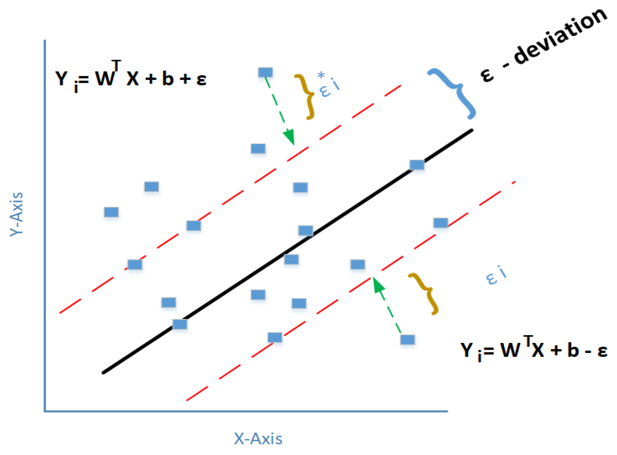
3.1. Support Vector Machine with Bayesian Optimization for Regression

A SVM for regression is one of the well-known machine learning methods that was first introduced by Drucker et al. [29]. SVM has been widely adopted for various regression problems and has achieved results with high accuracy when compared to other machine learning models. SVM can provide predictions for small and high dimensional data, data with local minima, and nonlinear problems [30].
SVM is based on a mathematical basis and statistical learning approaches that can improve the generalization capability by employing the structural risk minimization (SRM) principle [29,30].
For the training dataset Y = {( a 1 , b 1 ), ( a 2 , b 2 ), ( a 3 , b 3 ), …, ( a n , b n )}, a i , b I   R, where a i represents the feature vector of the input sample and b i is the corresponding labels to each sample for i = 1, 2, 3, …, n. The fundamental concept of SVM is to build a nonlinear map between output and input and then map the input data into the high dimensional feature space from low dimension using kernel as a function. A simple SVM model is shown in Figure 1.
f ( a ) = w . φ ( x ) + b
where φ ( x ) is a nonlinear function in which a low dimension feature input will be converted into high dimensional feature space. In SVM, W contains the coefficients of the data, and b is the learnable constant. The SVM objective function can be formulated as:
m i n   w , b ,   ε i , ε * i     1 2 | | w | | 2 + c   1 = 1 n ( ε i + ε i * )    
s u b j e c t   t o { f ( a ) i y i   ε + ε i     y i f ( a i ) ε + ε i * ε i 0 , ε i * 0 , i = 1 , 2 , , n .      
In the above equation where ε i * and ε i are the upper and lower slack variables. This is subject to ε –deviation y i f ( a i ) ε , the term 1 2 | | w | | 2 is a regularization that improves the generalization of the model.
The regularization constant parameter C determines the trade-off between experiential error and believing risk. In Equation (3), the ε denotes the loss parameter. Equation (2) constraint suggests that the loss will be ignored if the difference between the real and predicted values is less than ε . As shown in Figure 1, the actual value of the data a i is under the ε , where the chance of getting an error is quite a low estimate as zero. On the other hand, if the actual values b i are outside the ε   , then the error will be ε i   o r   ε i * .
Machine learning models are prone to underfitting and overfitting during a training phase. Thus, to avoid this problem, the regularization term, 1 2 | | w | | 2 as well as c   ,   the training error is minimized [30] Hyperparameters play an important role in fine-tuning the performance of machine learning models [31]. The tuning of hyperparameters can be either a manual or optimized approach. Manual approaches are time-consuming and may not achieve optimal performance. Due to this, various optimization approaches can be integrated into the selection of hyperparameters of machine learning models such as Bayesian optimization, heuristical optimization approaches, random search, and grid search methods. In this research, Bayesian optimization is utilized to optimize the hyperparameters of the SVM model.

3.2. Bayesian Optimization

In the Bayesian theory concept, by calculating the objective function of the posterior distribution, which captures the updated belief for the known objective function. For objective function f(a), Bayesian optimization constructs a probabilistic model. The model is exploited to predict the unknown next point to evaluate the bounded set A. From the preceding evaluation f(a) to make full use of predicted information and is not limited only on the Hessian approximations or local gradient, it can also find the maximum complex of non-convex functions [32].
There are two-parts that play a role with Bayesian optimization. The first one is the Gaussian process prior and the second one is the acquisition function that is used to evaluate the subsequent point by constructing a utility function.
The Gaussian process is an effective and powerful prior distribution over the space smooth function. It is based on a random variable that has no limit (e.g., an infinite number), where any finite random variable is subjective to combined Gaussian distribution [32].
The Gaussian distribution (GP) is expressed as:
f ( a ) ~ G P ( µ ( a ) , k ( a , a * ) )
where µ ( a ) is a mean function of a and the k ( a , a * ) value data is a covariance function of data a , a * .
There are many ways to choose an acquisition function like expected improvement (EI) as well as probability of improvement (PI). The PI function is written as
α P I ( a ) = ϕ ( ɤ ( a ) ) , ( ɤ ( a ) ) = f ( a b e s t ) μ ( a ) σ ( a )
where σ ( a ) and μ ( a ) indicate the predictive variance and mean function of the objective function.
Φ(.) and ɤ(.) express the PDF as well as CDF of standard normal distribution. The current best observation is donated by a b e s t = a r g   m a x   a i   a 1 : t f ( a i ) , respectively. In the SVM model, there are three parameters (C, ϵ, σ) to optimize, where C is the penalization coefficient; the kernel parameter is denoted by σ, when σ value is larger, the structural risk will be small; and ϵ is the insensitive loss coefficient that controls the gap (width) of the regression function on the insensitive area [33].

4. Results and Discussion

Table 2 illustrates twenty-four experiments with varied cutting parameters that were carried out under dry conditions. The trials were performed in a single-path double-pass system. Based on the second pass in each pass, the response was computed. This was provided to facilitate considerable wear for a 709M40 steel alloy to take place with 24 experimental trials. Scanning images of the nose wear were measured by field-emission scanning electron microscope (FESEM), as shown in Figure 1. The figure illustrates the micrographs of nose wear for different cutting speeds and feed rates. Nose wear was found to be the dominant wear mechanism than the flank and crater wear [34]. Figure 2 shows a comparison of tool edge performance in three experiments where low, moderate, and high cutting speed are used in association with a moderate feed of 0.2 mm/rev and a depth of 2.25 mm. To match the practical rough turning operations, nose wear was considered as a criteria in the experiment. A Zeiss Gemini SEM 500 field emission scanning electron microscope (FESEM) equipped with an energy-dispersive X-ray (EDX) microanalysis system was utilized to examine the worn tool inserts.

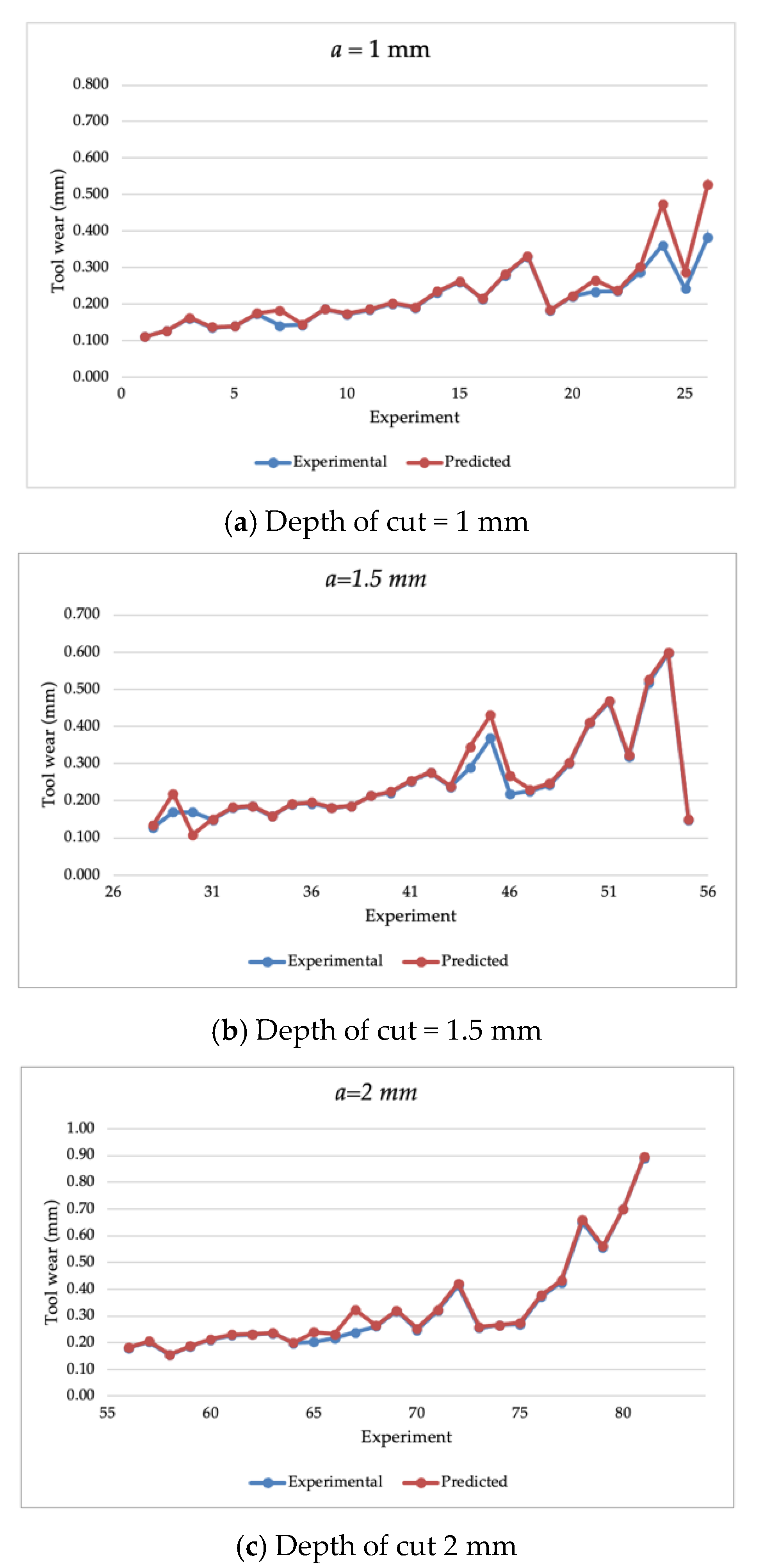
4.1. Training Dataset

To train the SVM model for determining the tool wear, data from experiments in the literature were extracted. Table A1 depicts the training data from [5] that was used to train the SVM model on the different feed rate, depth of cut, and cutting speed. It can be seen that the training data had 82 experiments for the CVD coated tool and similarly for the PVD coated tool, it added to a total of 162 experiments for the training dataset. The depth of cut ( d ) ,   feed rate ( f ) , and cutting speed ( V ) were considered as the input parameters whereas the wear of the cutting tool insert was considered as the response. The selection of the training dataset was based on the large numbers of experiments presented in [5], where large datasets are preferable in training artificial intelligence algorithms. In addition, the data present the input parameters of interests such as depth of cut, feed rate, and cutting speed with a comparable range, in terms of standard deviation of depth of cut, to our conducted experiment of the validation dataset of Table 2.
The SVM with the Bayesian optimization model was executed with an acquisition function defined as the probability of improvement with 30 iterations. Figure 3 illustrates the estimation of the tool wear of the CVD-coated cutting tool wear of the training dataset, while Figure 4 presents the estimation of the cutting tool wear of the PVD coated tool wear of the training dataset. It can be observed that the SVM model with Bayesian optimization achieved a high extent of accuracy by closely estimating the experimental training dataset. Table A2 presents the estimated value of the tool wear parameter of each experiment in the training dataset. To further assess the performance of the estimation results, statistical measures were calculated as the MAPE (“mean absolute percentage error”), RMSE (“root mean square error”), and CVRMSE (“coefficient of variation of root mean square error”), which are calculated in Equations (6)–(8), respectively, as:
M A P E = 1 n i = 1 n | y ^ i y i y i | × 100 %  
R M S E = i = 1 n ( y ^ i y i ) 2 n
C V R M S E = i = 1 n ( y ^ i y i ) 2 y ˘
where y denotes the experimental data point; y ^   denotes the estimated data point; and y ˘ as the average value. Table 3 presented the calculated performance metrics of the SVM model with Bayesian optimization for the training dataset. The model resulted in superior performance in terms of the MAPE, RMSE, and CVRMSE with an average of 5.36%, 2.48%, and 15.9%, respectively.

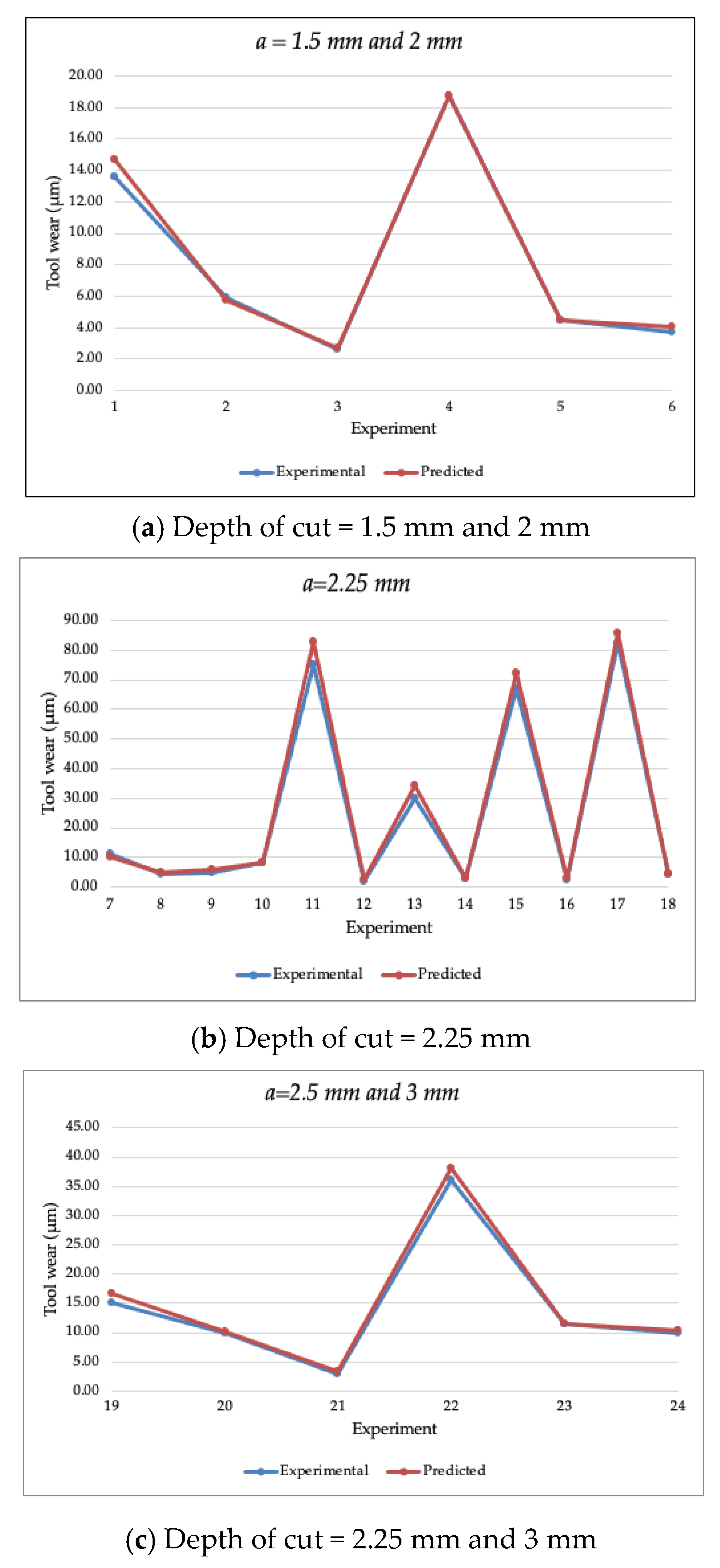
4.2. Validation Dataset

The promising trained model was then exported and used to estimate the cutting tool wear of the validation dataset that was presented in Table 2. Figure 5 illustrates the experimental and predicted data of the cutting tool wear of the validation dataset with various depths of cuts of 1.5 mm, 2 mm, 2.25 mm, 2.5 mm, and 3 mm. The estimated data points by the SVM model with Bayesian optimization closely matched the experimental data points of the validation dataset. Table 4 depicts the estimated individual values of the cutting tool wear parameter for each experiment in the validation dataset. The performance metrics of the SVM model with Bayesian optimization on the validation dataset were calculated and are presented in Table 5. It can be noted that the proposed SVM model achieved a high extent of accuracy in estimating the cutting tool wear parameter of the validation dataset with a MAPE of 6.13%, RMSE of 2.29%, and CVRMSE of 9.02%. The results validate the model performance and the feasibility of estimating the cutting tool wear computationally based on the previous training dataset and thus can reduce the experimental work and resources.

5. Conclusions

This research explored the performance of the artificial intelligence-based estimation approach of tool wear in a turning process of 709M40 alloy steel. Support vector machine for regression with Bayesian optimization model was employed to estimate the tool wear value based on the depth of cut and cutting speed as well as feed rate inputs. The proposed model was trained on a training dataset of 162 data points and was then used to determine the tool wear of our validation dataset. The reported results suggest the feasibility of the SVM model in estimating the tool wear with high accuracy of MAPE of 6.13%, RMSE of 2.29%, and CVRMSE of 9.02% for the validation dataset. The estimated values closely match the conducted experimental tool wear values. The approach was validated for the 709M40 alloy steel based on depth of cut, feed rate, and cutting speed for a certain range of values. For other materials with a different range of input values, it would require retraining the algorithm using the transfer learning approach. The proposed approach contributes more toward saving the cost, time, and labor in the manufacturing process. Moreover, adopting artificial intelligence estimation methods saves resources and enables more efficient and sustainable manufacturing processes.

Author Contributions

Methodology, A.M.A. and M.S.A.; Conceptualization, A.M.A. and M.S.A.; Validation, A.M.A. and M.S.A.; Software, A.M.A. and M.S.A.; Formal analysis, A.M.A. and M.S.A.; Investigation, A.M.A. and M.S.A.; Resources, A.M.A. and M.S.A.; Data curation, A.M.A. and M.S.A.; Draft preparation of writing-original, A.M.A. and M.S.A.; Editing & review writing, A.M.A. and M.S.A.; Visualization, A.M.A. and M.S.A. All authors have read and agreed to the published version of the manuscript.

Funding

This research received no external funding.

Institutional Review Board Statement

Not applicable.

Informed Consent Statement

Not applicable.

Data Availability Statement

The data presented in this study are available on request from the corresponding author.

Conflicts of Interest

The authors declare no conflict of interest.

Nomenclature

VCutting Speed (m/min)
fFeed Rate (mm/rev)
dDepth of Cut (mm)
RaSurface Roughness (µm/m)
MAEMean Root Square Error
RMSERoot Mean Square Error
NwNose Tool Wear (µm/min)
CVRMSECoefficient of the Variation of the Root Mean Square Error

Appendix A

Table A1. Training data of various cutting parameters to train the SVM model [5].
Exp
No.
Cutting
Parameters
Cutting
Length
CVD Coated
Tool
PVD Coated
WC
d [mm]V [m/min]f [mm/rev]L [mm]Ra [μ/m] N w   [ μ / min ] Ra [ μ/m] N w   [ μ / min ]
11300.052401.820.1101.320.047
21300.052801.940.1271.540.079
31300.0521202.120.161.680.083
41300.104402.150.13520.07
51300.104802.180.1392.40.092
61300.1041202.480.1732.60.093
71300.162403.30.143.720.086
81300.162803.60.1434.10.093
91300.1621203.80.1864.180.094
101600.052401.760.1721.30.11
111600.052801.90.1841.450.12
121600.0521202.040.2011.50.123
131600.104401.90.1891.760.115
141600.104802.10.2321.980.126
151600.1041202.30.2612.160.132
161600.162403.50.2144.120.121
171600.162803.850.2794.220.128
181600.1621204.10.3304.340.15
191900.052401.40.1831.280.121
201900.052801.60.2211.40.21
211900.0521202.30.2341.680.308
221900.104402.250.2351.940.19
231900.104802.30.2872.240.283
241900.1041202.70.3612.440.321
251900.1624040.2424.680.201
261900.162804.30.3834.740.297
271900.1621204.90.5865.080.38
281.5300.052402.040.1282.020.086
291.5300.052802.10.1692.20.112
301.5300.0521202.150.172.40.116
311.5300.104402.180.1482.240.115
321.5300.104802.20.182.320.121
331.5300.1041202.580.1852.720.132
341.5300.162403.640.1584.160.126
351.5300.162804.240.194.320.142
361.5300.1621204.50.1934.40.148
371.5600.052401.820.1811.640.111
381.5600.052801.980.1861.70.129
391.5600.0521202.060.2141.860.14
401.5600.104402.080.22120.126
411.5600.104802.150.2522.260.138
421.5600.1041202.470.2762.40.16
431.5600.162404.160.2374.180.178
441.5600.162804.320.2894.40.207
451.5600.1621204.750.3694.520.253
461.5900.052402.40.2181.940.177
471.5900.052802.580.22620.36
481.5900.0521202.60.2432.060.567
491.5900.104402.470.32.20.313
501.5900.104802.540.4092.360.376
511.5900.1041203.160.4663.020.597
521.5900.162404.160.3184.220.331
531.5900.162804.780.5174.60.507
541.5900.1621205.10.5975.260.602
552300.052402.380.1472.40.09
562300.052802.390.182.450.12
572300.0521202.60.2032.80.123
582300.104402.40.1542.650.126
592300.104802.520.1862.760.13
602300.1041202.640.2102.920.134
612300.162404.120.2274.460.135
622300.162804.450.234.980.175
632300.1621204.650.2355.060.183
642600.052401.980.1992.250.123
652600.052802.10.2032.30.15
662600.0521202.450.2162.440.256
672600.104402.460.2382.680.133
682600.104802.620.2612.890.275
692600.1041202.840.3183.010.47
702600.162404.650.2484.680.184
712600.162804.70.325.10.425
722600.1621204.760.4155.560.56
732900.052402.40.2552.30.273
742900.052802.420.2652.380.454
752900.0521202.680.2692.750.620
762900.104402.540.3722.920.390
772900.104802.70.4253.240.56
782900.1041203.20.6503.450.680
792900.162404.980.5555.340.412
802900.162805.020.75.550.601
812900.1621205.40.8915.920.710
Table A2. Estimated cutting tool wear parameter of the training dataset.
Exp
Num
CVD CoatedPVD Coated
ExperimentalSVMExperimentalSVM
N w   [ μ / m ] N w   [ μ / m ] N w   [ μ / m ] N w   [ μ / m ]
10.1100.1100.0470.083
20.1270.1280.0790.082
30.160.1630.0830.086
40.1350.1370.070.072
50.1390.1400.0920.086
60.1730.1750.0930.094
70.140.1820.0860.092
80.1430.1450.0930.092
90.1860.1860.0940.093
100.1720.1730.110.109
110.1840.1860.120.119
120.2010.2030.1230.121
130.1890.1910.1150.114
140.2320.2360.1260.125
150.2610.2630.1320.131
160.2140.2150.1210.120
170.2790.2820.1280.127
180.3300.3320.150.149
190.1830.1840.1210.120
200.2210.2230.210.217
210.2340.2660.3080.289
220.2350.2370.190.178
230.2870.3030.2830.280
240.3610.4730.3210.320
250.2420.2880.2010.200
260.3830.5280.2970.296
270.5860.6870.380.377
280.1280.1350.0860.085
290.1690.2200.1120.111
300.170.1080.1160.116
310.1480.1500.1150.114
320.180.1830.1210.119
330.1850.1860.1320.129
340.1580.1600.1260.124
350.190.1910.1420.134
360.1930.1960.1480.139
370.1810.1810.1110.104
380.1860.1860.1290.121
390.2140.2140.140.151
400.2210.2240.1260.103
410.2520.2550.1380.143
420.2760.2760.160.190
430.2370.2390.1780.163
440.2890.3460.2070.217
450.3690.4310.2530.272
460.2180.2670.1770.189
470.2260.2300.360.348
480.2430.2470.5670.561
490.30.3040.3130.311
500.4090.4110.3760.376
510.4660.4690.5970.590
520.3180.3220.3310.327
530.5170.5260.5070.501
540.5970.6000.6020.596
550.1470.1490.090.088
560.180.1820.120.119
570.2030.2050.1230.121
580.1540.1550.1260.124
590.1860.1880.130.128
600.2100.2130.1340.123
610.2270.2310.1350.151
620.230.2310.1750.167
630.2350.2360.1830.191
640.1990.1990.1230.044
650.2030.2400.150.140
660.2160.2320.2560.263
670.2380.3240.1330.137
680.2610.2650.2750.272
690.3180.3220.470.413
700.2480.2530.1840.299
710.320.3240.4250.419
720.4150.4210.560.531
730.2550.2590.2730.265
740.2650.2660.4540.448
750.2690.2740.6200.590
760.3720.3780.3900.390
770.4250.4320.560.553
780.6500.6600.6800.680
790.5550.5610.4120.407
800.70.7010.6010.592
810.8910.8950.7100.699

References

  1. Bagga, P.J.; Makhesana, M.A.; Patel, K.M. Tool wear monitoring in turning using image processing techniques. Mater. Today Proc. 2021, 44, 771–775. [Google Scholar] [CrossRef]
  2. Amrita, M.A.; Rukmini Srikant, R.; VSN, V. Optimisation of cutting parameters for cutting temperature and tool wear in turning AISI4140 under different cooling conditions. Adv. Mater. Process. Technol. 2020, 2020, 1–19. [Google Scholar]
  3. Qian, Y.; Tian, J.; Liu, L.; Zhang, Y.; Chen, Y. A tool wear predictive model based on SVM. In Proceedings of the 2010 Chinese Control and Decision Conference, Xuzhou, China, 26–28 May 2010; pp. 1213–1217. [Google Scholar]
  4. Babu, M.P.; Prasad, B.S. Experimental Investigation to Predict Tool Wear and Vibration Displacement in Turning—A Base for Tool Condition Monitoring. J. Manuf. Sci. Prod. 2016, 16, 103–114. [Google Scholar] [CrossRef]
  5. Çelik, Y.H.; Kilickap, E.; Güney, M. Investigation of cutting parameters affecting on tool wear and surface roughness in dry turning of Ti-6Al-4V using CVD and PVD coated tools. J. Braz. Soc. Mech. Sci. Eng. 2017, 39, 2085–2093. [Google Scholar] [CrossRef]
  6. Kuntoğlu, M.; Sağlam, H. Investigation of progressive tool wear for determining of optimized machining parameters in turning. Measurement 2019, 140, 427–436. [Google Scholar] [CrossRef]
  7. Alajmi, M.S.; Almeshal, A.M. Prediction and Optimization of Surface Roughness in a Turning Process Using the ANFIS-QPSO Method. Materials 2020, 13, 2986. [Google Scholar] [CrossRef]
  8. Pourmostaghimi, V.; Zadshakoyan, M.; Badamchizadeh, M.A. Intelligent model-based optimization of cutting parameters for high-quality turning of hardened AISI D2. Artif. Intell. Eng. Des. Anal. Manuf. 2020, 34, 1–9. [Google Scholar] [CrossRef]
  9. Kong, D.; Chen, Y.; Li, N.; Duan, C.; Lu, L.; Chen, D. Relevance vector machine for tool wear prediction. Mech. Syst. Signal Process. 2019, 127, 573–594. [Google Scholar] [CrossRef]
  10. Alajmi, M.S.; Almeshal, A.M. Predicting the Tool Wear of a Drilling Process Using Novel Machine Learning XGBoost-SDA. Materials 2020, 13, 4952. [Google Scholar] [CrossRef] [PubMed]
  11. Alajmi, M.S.; Almeshal, A.M. Modeling of Cutting Force in the Turning of AISI 4340 Using Gaussian Process Regression Algorithm. Appl. Sci. 2021, 11, 4055. [Google Scholar] [CrossRef]
  12. Alajmi, M.S.; Almeshal, A.M. Least Squares Boosting Ensemble and Quantum-Behaved Particle Swarm Optimization for Predicting the Surface Roughness in Face Milling Process of Aluminum Material. Appl. Sci. 2021, 11, 2126. [Google Scholar] [CrossRef]
  13. Jurkovic, Z.; Cukor, G.; Brezocnik, M.; Brajkovic, T. A comparison of machine learning methods for cutting parameters prediction in high-speed turning process. J. Intell. Manuf. 2018, 29, 1683–1693. [Google Scholar] [CrossRef]
  14. Twardowski, P.; Wiciak-Pikuła, M. Prediction of Tool Wear Using Artificial Neural Networks during Turning of Hardened Steel. Materials 2019, 12, 3091. [Google Scholar] [CrossRef] [Green Version]
  15. McParland, D.; Baron, S.; O’Rourke, S.; Dowling, D.; Ahearne, E.; Parnell, A. Prediction of tool-wear in turning of medical grade cobalt chromium molybdenum alloy (ASTM F75) using non-parametric Bayesian models. J. Intell. Manuf. 2019, 30, 1259–1270. [Google Scholar] [CrossRef] [Green Version]
  16. Wang, J.; Yan, J.; Li, C.; Gao, R.X.; Zhao, R. Deep heterogeneous GRU model for predictive analytics in smart manufacturing: Application to tool wear prediction. Comput. Ind. 2019, 111, 1–14. [Google Scholar] [CrossRef]
  17. Sheng, J. A modeling method for turning parameters coupling based on minimum cutting tool wear. Int. J. Adv. Manuf. Technol. 2015, 76, 705–712. [Google Scholar] [CrossRef]
  18. Zheng, G.; Xu, R.; Cheng, X.; Zhao, G.; Li, L.; Zhao, J. Effect of cutting parameters on wear behavior of coated tool and surface roughness in high-speed turning of 300M. Measurement 2018, 125, 99–108. [Google Scholar] [CrossRef]
  19. D’Addona, D.M.; Ullah, A.M.M.S.; Matarazzo, D. Tool-wear prediction and pattern-recognition using artificial neural network and DNA-based computing. J. Intell. Manuf. 2015, 28, 1285–1301. [Google Scholar] [CrossRef]
  20. Chang, W.; Wu, S.; Hsu, J. Investigated iterative convergences of neural network for prediction turning tool wear. Int. J. Adv. Manuf. Technol. 2020, 106, 2939–2948. [Google Scholar] [CrossRef]
  21. Wang, J.; Li, Y.; Zhao, R.; Gao, R.X. Physics guided neural network for machining tool wear prediction. J. Manuf. Syst. 2020, 57, 298–310. [Google Scholar] [CrossRef]
  22. Chen, Y.; Jin, Y.; Jiri, G. Predicting tool wear with multi-sensor data using deep belief networks. Int. J. Adv. Manuf. Technol. 2018, 99, 1917–1926. [Google Scholar] [CrossRef]
  23. Wu, X.; Li, J.; Jin, Y.; Zheng, S. Modeling and analysis of tool wear prediction based on SVD and BiLSTM. Int. J. Adv. Manuf. Technol. 2020, 106, 4391–4399. [Google Scholar] [CrossRef]
  24. Shen, Y.; Yang, F.; Habibullah, M.S.; Ahmed, J.; Das, A.K.; Zhou, Y.; Ho, C.L. Predicting tool wear size across multi-cutting conditions using advanced machine learning techniques. J. Intell. Manuf. 2020, 2020, 1–14. [Google Scholar] [CrossRef]
  25. Sandvik Tools Catalog, Sandvik Coromant. 2021. Available online: https://www.sandvik.coromant.com/en-gb/downloads (accessed on 24 June 2021).
  26. Geethanjali, K.S.; Ramesha, C.M.; Chandan, B.R. Comparative Studies on Machinability of MCLA Steels EN19 and EN24 Using Taguchi Optimization Techniques. Mater. Today Proc. 2018, 5, 25705–25712. [Google Scholar] [CrossRef]
  27. West York Steel 709M40 Alloy Steel Datasheet, West York Steel. 2021. Available online: https://www.westyorkssteel.com/files/709m40.pdf (accessed on 24 June 2021).
  28. Steel Grades Online Database. 2021. Available online: https://www.steel-grades.com/Steel-Grades/specialsteel/74/7897/709M40.html (accessed on 24 June 2021).
  29. Drucker, H.; Burges, C.J.; Kaufman, L.; Smola, A.J.; Vapnik, V. Support vector regression machines. Adv. Neural Inf. Process. Syst. 1996, 28, 779–784. [Google Scholar]
  30. Guo, Y.; Li, X.; Bai, G.; Ma, J. Time Series Prediction Method Based on LS-SVR with Modified Gaussian RBF. In Proceedings of the International Conference on Neural Information Processing, Lake Tahoe, NV, USA, 3–6 December 2012; pp. 9–17. [Google Scholar]
  31. Teh, Y.W.; Seeger, M.; Jordan, M. Semiparametric latent factor models. In Proceedings of the Tenth International Workshop on Artificial Intelligence and Statistics, Savannah, Georgia, Bridgetown, Barbados, 6–8 January 2005; pp. 565–568. [Google Scholar]
  32. Rasmussen, C.E.; Williams, C.K.I. Gaussian Processes for Machine Learning; MIT Press: Cambridge, MA, USA, 2006; p. 68. [Google Scholar]
  33. Wang, D.; Wang, C.; Xiao, J.; Xiao, Z.; Chen, W.; Havyarimana, V. Bayesian optimization of support vector machine for regression prediction of short-term traffic flow. Intell. Data Anal. 2019, 23, 481–497. [Google Scholar] [CrossRef]
  34. Sonawane, G.D.; Sargade, V.G. Evaluation and multi-objective optimization of nose wear, surface roughness and cutting forces using grey relation analysis (GRA). J. Braz. Soc. Mech. Sci. Eng. 2019, 41, 557. [Google Scholar] [CrossRef]
Figure 1. Support vector regression model.
Materials 14 03773 g001
Figure 2. Micrographs of nose wear for different cutting speeds and feed rates.
Materials 14 03773 g002
Figure 3. The estimated tool wear of the training dataset parameters in the CVD coated cutting tool with a depth of cut of (a) 1 mm, (b) 1.5 mm, and (c) 2 mm.
Materials 14 03773 g003
Figure 4. The estimated tool wear of the training dataset of a PVD cutting tool with a depth of cut of (a) 1 mm, (b) 1.5 mm, and (c) 2 mm.
Materials 14 03773 g004
Figure 5. The estimated tool wear of the validation dataset with the various depth of cuts of (a) 1.5 mm and 2 mm, (b) 2.25 mm, and (c) 2.25 mm and 3 mm.
Materials 14 03773 g005
Table 1. Chemical composition, mechanical, and physical properties of the 709M40 alloy steel [27,28].
Composition(Wt%)Mechanical PropertiesValues
C 0.44Tensile strength N / mm 2 850–1000
C r 0.99 Yield   Strength   N / mm 2 650
M o 0.25Hardness ( H B ) 248–302
M n 0.85Elongation %13
S <0.04Impact test ( KV ) 50
P <0.04Density ( Kg dm 3 ) 421
Table 2. The experimental data.
Experiment Trial V
[m/min]
f
[mm/rev]
d [mm] N w
[µm/min]
T1102.670.21.513.6
T2103.40.21.55.88
T372.350.1222.65
T41450.3218.75
T5148.220.1224.48
T672.690.323.7
T71040.22.2511
T8104.720.22.254.6
T9103.670.22.255
T10103.060.22.258.33
T112060.22.2575
T12500.22.252.14
T13101.710.62.2530
T14104.150.062.252.91
T152060.22.2566.7
T1650.360.22.252.5
T17103.550.62.2582.41
T18104.80.062.254.55
T19145.890.122.515
T20720.32.510
T2172.320.122.52.97
T22144.720.32.536.14
T23104.660.2311.54
T24103.750.2310
Table 3. Statistical performance metrics of the SVM model with Bayesian optimization for the training dataset.
MetricTraining Dataset
PVD CoatedCVD Coated
MAPE %5.6305.096
RMSE %1.9363.040
CVRMSE %11.61920.326
Table 4. The estimated cutting tool wear of the validation dataset.
DataActual
N w   [ μ m / m ]
Estimated
N w   [ μ m / m ]
113.6014.683
25.885.731
32.652.736
418.7518.691
54.484.492
63.704.046
711.0010.385
84.604.681
95.005.684
108.338.463
1175.0082.834
122.142.309
1330.0033.981
142.912.994
1566.7072.202
162.502.928
1782.4185.384
184.554.607
1915.0016.600
2010.0010.211
212.973.354
2236.1438.199
2311.5411.472
2410.0010.354
Table 5. Statistical performance metrics of the SVM model with Bayesian optimization for the validation dataset.
MetricValidation Dataset
MAPE %6.13
RMSE %2.29
CVRMSE %9.02
Publisher’s Note: MDPI stays neutral with regard to jurisdictional claims in published maps and institutional affiliations.

