2. Statement of the Problem and Basic Equations
Consider a long open-ended cylinder of initial yield stress
, Young’s modulus
E, Poisson’s ratio υ, outer radius
, and inner radius
. The cylinder is subject to uniform pressure
over its inner radius, followed by unloading. The pressure is sufficient to yield the material to an intermediate radius
at loading and
in reversed flow. The outer radius of the cylinder is stress-free.
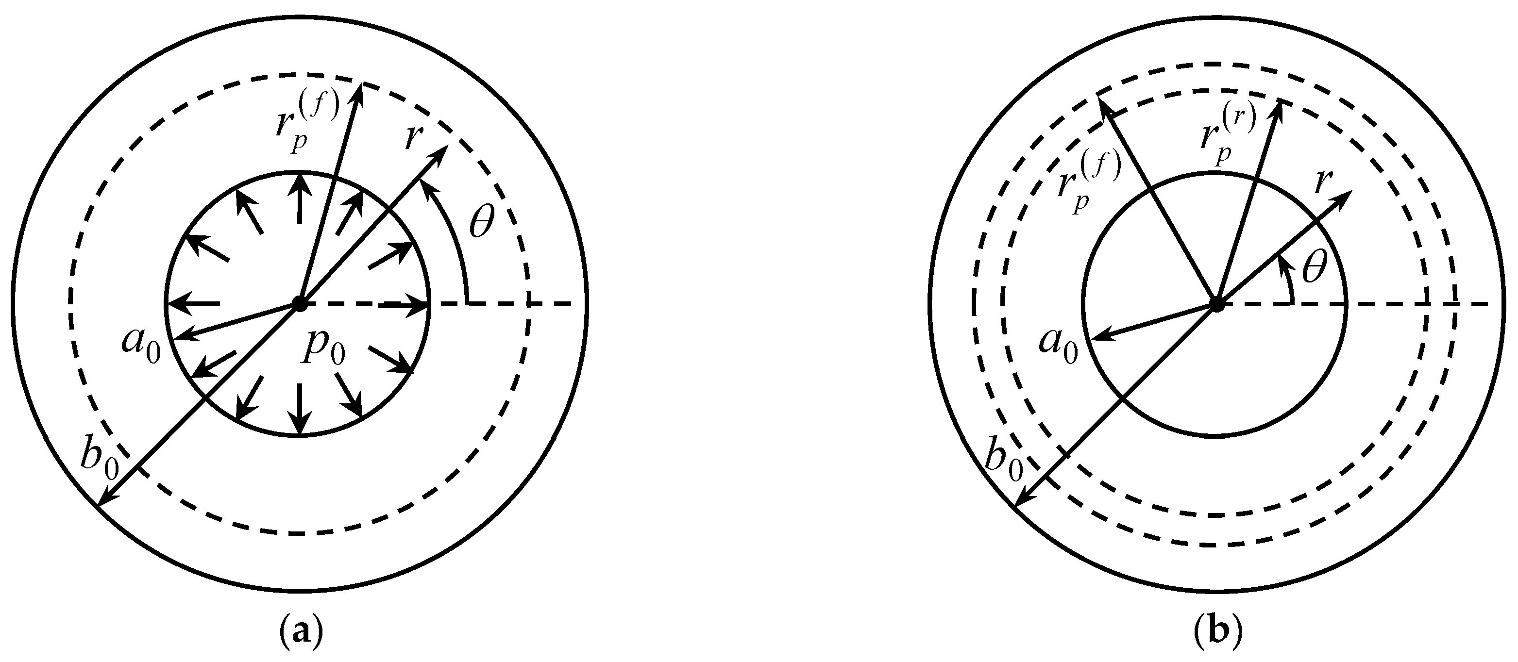
Figure 1 illustrates the boundary value problem. It is natural to use the cylindrical coordinate system
, as shown in this figure. The solution is independent of
, and the principal stress trajectories coincide with the coordinate curves of this coordinate system. The normal stresses referred to the cylindrical coordinate system, which are the principal stresses, are denoted as
,
and
. Moreover, it is assumed that the state of stress is plane stress such that
.
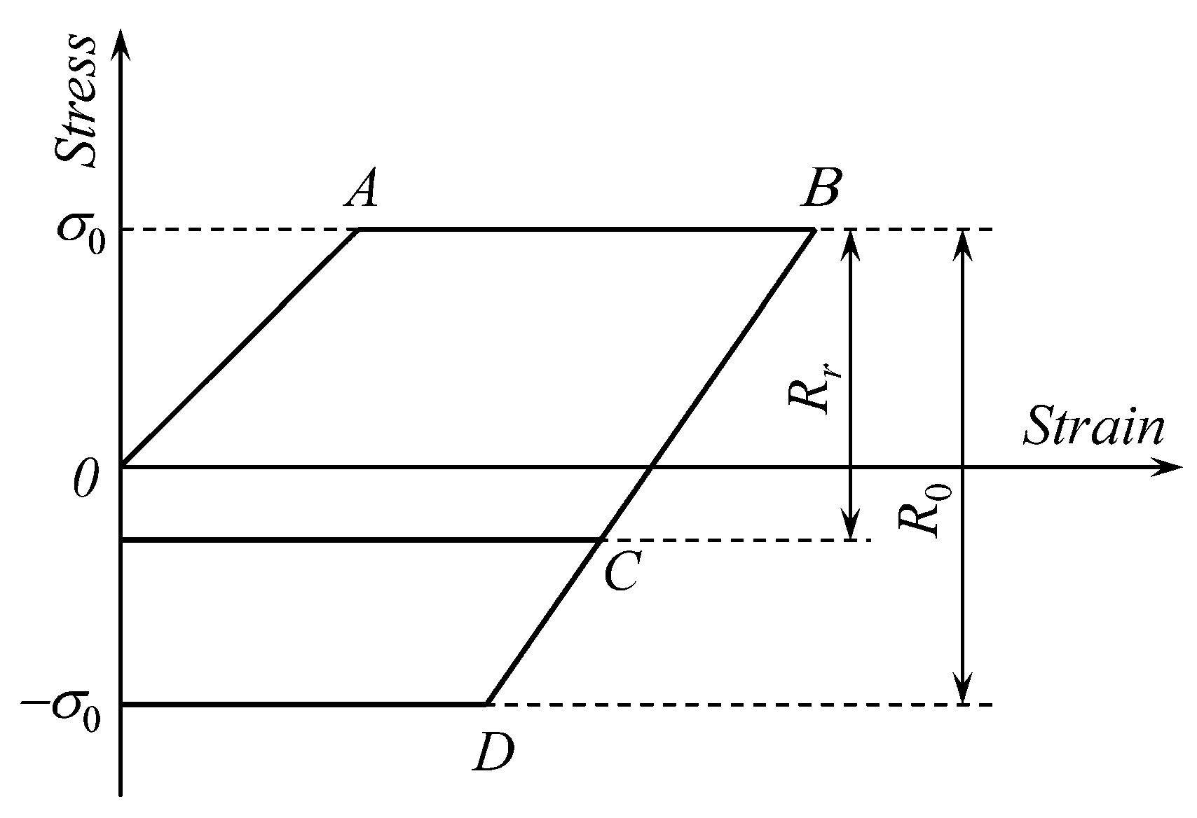
A general feature of the class of materials considered in the present paper is that there is little or no forward hardening, but a significant Bauschinger effect. This feature of constitutive material behavior is illustrated in
Figure 2 for one-dimensional loading. Forward deformation is represented by the line
OAB, where
OA corresponds to elastic deformation and
AB to elastic/plastic deformation. Line
BD represents the elastic unloading in materials with no Bauschinger effect. In this case, the elastic range is
R0. Line
BC represents the elastic unloading in materials that reveal a Bauschinger effect. In this case, the elastic range becomes
Rr where
Rr <
R0.
Taking into account the discussion above, the constitutive equations at loading constitute Hooke’s law, a yield criterion of perfect plasticity under plane stress conditions and its associated flow rule. In particular, the von Mises yield criterion under plane stress conditions takes the form
Let
,
and
be the plastic strain components referred to the cylindrical coordinate system. Then, the plastic flow rule is
Here,
is the hydrostatic stress,
,
is a non-negative multiplier, and the superimposed dot denotes the derivative with respect to a time-like parameter,
t. The elastic strain components,
,
and
, are connected to the stress components as
The components of the total strain tensor are
It is assumed that the forward plastic strain components affect the reversed yield criterion. In particular, according to Prager’s law [
21], the reversed yield criterion under plane stress conditions is
where
C is a material constant. The plastic flow rule associated with the yield criterion (5) is
Here, and in the solution for the stage of unloading, the superscript f denotes the forward strain.
The constitutive equations above should be supplemented with the only non-trivial equilibrium equation:
It is convenient to use the following dimensionless quantities:
In particular, Equation (7) becomes
The boundary conditions at the stage of forward loading are
and
The boundary conditions at the stage of unloading are
and
Here is the increment of the radial stress in the course of unloading and is the value of p at the end of loading.
The material model above has been proposed in [
9].
3. Solution at Loading
A solution at loading has been proposed in [
20]. This solution is outlined in this section to supply the equations that are necessary for determining the distribution of residual stresses after unloading. In what follows,
will denote the value of
p at the end of loading.
The general stress solution in the elastic region is well known [
10]. This solution, satisfying the boundary condition (11), is represented as
Here
A is a function of
p. The strain solution is immediate from (1), (3), (8), and (14). As a result,
The yield criterion (1) is satisfied by the following standard substitution:
Here,
is a new unknown function of
. Equations (9) and (16) combine to give
The distribution of the principal stresses is given by (14) in the range
and by (16) in the range
. Here,
is the dimensionless radius of the elastic/plastic interface. Then, using (16), one can rewrite the boundary condition (10) as
where
is the value of
at
. The solution of Equation (17) satisfying the boundary condition (18) is
Equations (16) and (19) supply the dependence of the stress components on the dimensionless radius in parametric form.
It is seen from (18) that
and
is a monotonic function of
p in the range
. Therefore, it is possible to assume with no loss of generality that
(
t has been introduced after Equation (2)). It is seen from (4) that
. The dependence of
on
in the plastic region is given by
Here,
is a dummy variable of integration and
is the value of
at
. The quantities
,
, and
are functions of
. Choose an arbitrary value of
in the range
. This value of
will denoted as
. At
,
is a function of
, as follows from (19). One can eliminate
in (20) using this function. Then, the right-hand side of (20) becomes a function of
,
. The resulting equation can be immediately integrated to give the value of the total circumferential strain at
at the end of loading as
Here, is the value of , at which , is determined from (18) at , and is the elastic circumferential strain at the elastic/plastic boundary at the instant when . The value of is found from (15). The elastic portion of the circumferential strain is determined from (3) and (16). Having found the elastic portion, the plastic portion of the circumferential strain is immediate from (4) and (21).
The plastic portions of the radial and axial strains can be found in a similar manner. In particular,
Since
at
, one can rewrite (22) as
These equations supply the forward plastic strains
and
at
and
. Using integration by parts, one transforms the equations in (23) to
It has been taken into account here that
at
. At
, one can eliminate
in the integrands in (24) using (19). The plastic portion of the circumferential strain is immediate from (21) and Hooke’s law. It remains to determine the derivative
at
. Since
, it follows from (19) that
Using (19) and (25), one can express the derivative as a function of . Then, the integrals in (24) can be evaluated.
A full description of this method of solution, including the system of equations for determining
,
,
,
, and
A as functions of
p, is provided in [
20]. In what follows, it is assumed that the solution at loading is available, including the plastic strains involved in (5) and (6).
It is worthy of note that all strains are proportional to k. This is seen from (15), (21), and (24). Therefore, the value of k is immaterial for theoretical solutions. In particular, assume that the solution for a cylinder of a given material is available. Then, simple scaling of this solution provides the solutions for similar cylinders of material with the same Poisson’s ratio but any value of k. For this reason, the solution in the next section will be derived in terms of , and instead of the strain components.
4. Stress Solution at Unloading
Using the general stress solution given in [
10], one can determine the increments of the principal stresses in the following form:
where
and
are new constants of integration. It follows from (12), (13) and (26) that
Substituting (27) into (26) gives
The yield criterion (5) can be rewritten as
where
. The solution (28) is valid if this inequality is not violated in the range
. The solution at loading and (28) show that it is sufficient to check (29) at
. It is evident from (10) and (12) that
at
. Using (16), (18) and (28) one can get
Substituting (30) and (31) into (29) one arrives at
The forward plastic strains are understood to be calculated at . The equation that follows from the equation has been used to derive (32). The equation follows immediately from (2).
Equations (31) and (32) combine to supply the equation for determining the maximum possible value of at which the process of unloading is purely elastic. This value of is denoted as . It is worthy of note that the values of , and involved in (32) depend on .
In what follows, it is assumed that
. Therefore, a reversed plastic region occurs in the course of unloading. The radius of this region is denoted as
(
Figure 1) and its dimensionless representation as
. The solution (26) is valid in the region
. However,
and
are not determined from (27). The yield criterion (5) is valid in the region
. This criterion is satisfied by the substitution
where
Furthermore,
is a new unknown function of
. Since
is a known monotonic function of
in the region
, Equation (9) can be rewritten as
One can eliminate the derivative
in this equation using (17). Then, Equation (35) becomes
Using (33) and (34), Equation (36) can be transformed into
Since
at
at the end of unloading, it follows from (33) and (34) that the boundary condition to Equation (37) is
where
is determined from
The forward plastic strains involved in the definitions of and are understood to be calculated at . Equation (37) should be solved numerically. It is worthy of note that the dependence of the third and fourth terms of this equation on is known from the solution at loading described in the previous section. Therefore, the solution of Equation (37) satisfying the boundary condition (38) supplies the dependence of on in the range .
The solution of (26) must satisfy the boundary condition (13). Therefore,
and Equation (26) becomes
This solution is valid in the region
. The distribution of the residual stresses in the region
is determined from (16) and (40) as
Here, one can eliminate
(or
) using (19). Both
and
must be continuous across the elastic/plastic boundary
. Then, it follows from (33), (34) and (41) that
The forward plastic strains involved in the definitions of
,
and
are understood to be calculated at
. Additionally,
and
are the values of
and
at
, respectively. One can eliminate
between the equations in (42) to arrive at
It follows from (19) that
Using (44), one can eliminate
in (43). The solution of Equation (37) supplies the dependence of
on
. As a result, Equation (43) contains one unknown
. This resulting equation should be solved for
numerically. Then,
is found from the solution of Equation (37) and
from (44). The value of
can be determined from any equation in (42). For example,
This equation should be used for eliminating in (41).
The distribution of the residual stresses in the region
is determined from (14) and (40) as
As before, in this equation should be eliminated by means of Equation (45).
The distribution of the residual stresses in the region
is determined as follows. One can transform Equations (33) and (34) to
In these equations, is a known function of due to the solution of Equation (37). Then, (19) and (47) supply the dependence of the residual stresses on in parametric form, with being the parameter.
The solution found is illustrated in
Figure 3 and
Figure 4 for an
cylinder and several values of
c. It has been assumed that
. The special case,
, corresponds to the material that reveals no Bauschinger effect. The stage of loading ends when
. The corresponding value of the internal pressure is
(approximately).
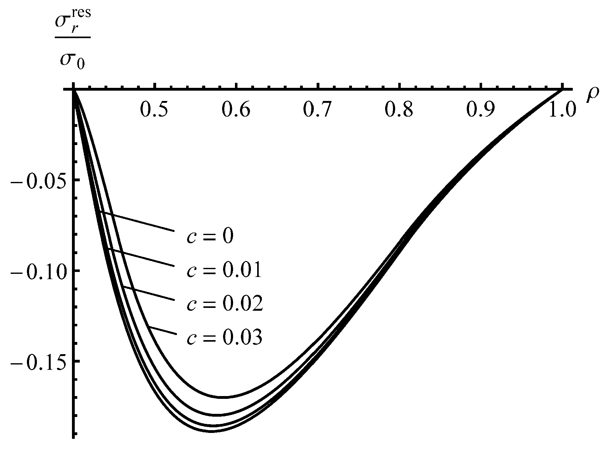
Figure 3 displays the variation of the residual radial stress with the dimensionless radius. The effect of the
c—value is not so significant. This is not surprising because the value of this stress at
and
is controlled by the boundary conditions.
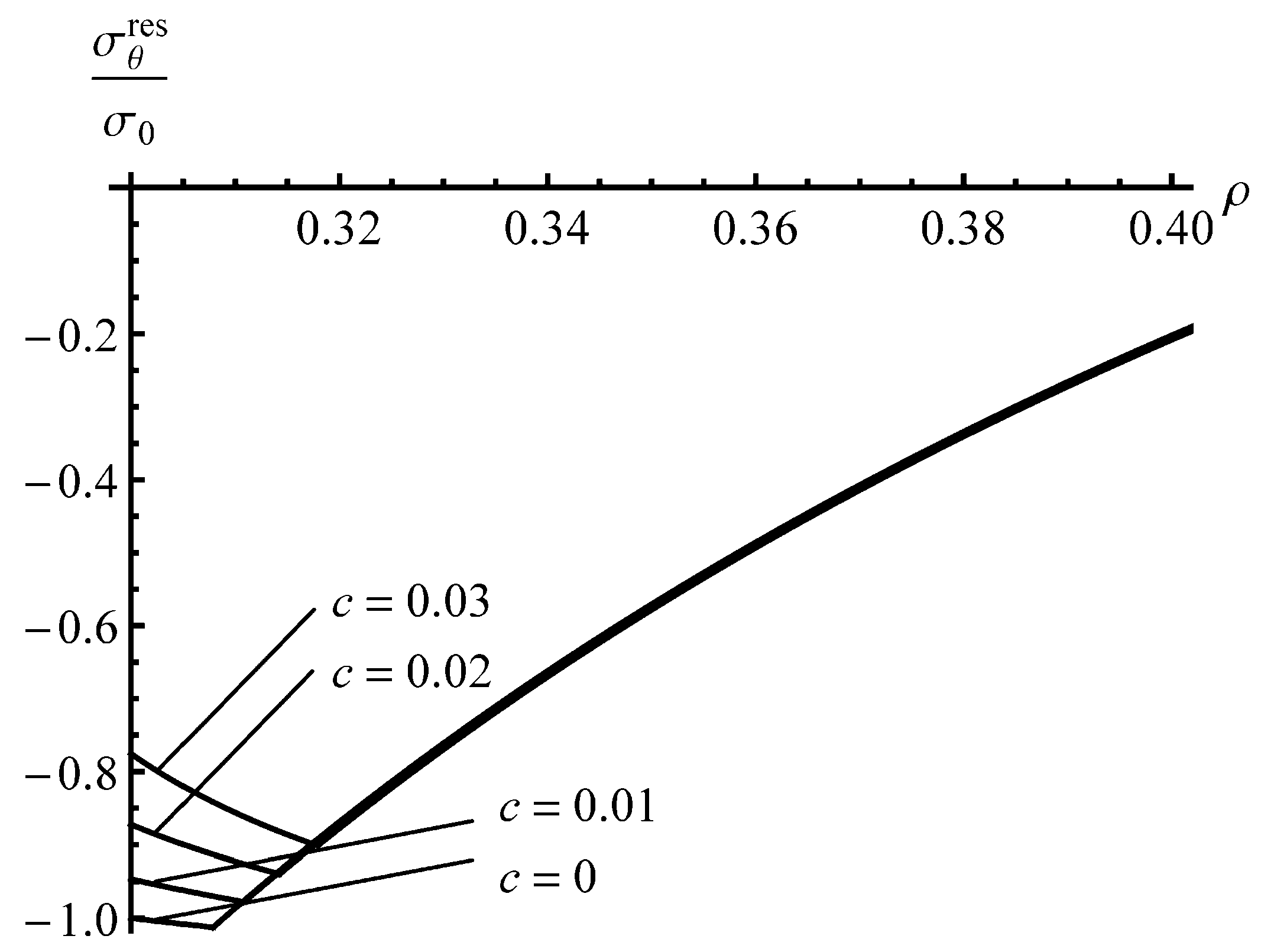
Figure 5 shows the variation in the residual circumferential stress with the dimensionless radius. The effect of the
c—value on this stress is significant in the vicinity of the inner radius where the magnitude of the circumferential stress is the most significant quantity in autofrettage technologies. It is seen from
Figure 3 that an increase in the Bauschinger effect leads to a decrease in the value of
at the inner radius of the cylinder, which has a negative impact on its performance under service conditions.
To reveal an effect of
a on the distribution of the residual stresses, the solution for an
cylinder has been found assuming that
. The effect of
c—value on the distribution of the residual radial stress is even smaller than that shown in
Figure 3. Therefore, the distribution of this stress at
is not illustrated. It is seen from
Figure 4 that the effect of
c—value on the distribution of the residual circumferential stress is negligible in the range
. Therefore,
Figure 4 shows the distribution of the residual circumferential stress near the inner radius of an
cylinder. It is seen from this figure that the Bauschinger effect has a significant impact on this stress near the inner radius. Comparison of the distributions of the residual circumferential stress near the inner radius for the
and
cylinders (
Figure 4 and
Figure 5) shows that the magnitude of this stress at
is sensitive to both
a and
c at the same value of
. It is worthy of note that there is no need to solve the boundary value problem at unloading to find the value of
at
.
It follows from (11) and (13) that
at
. Then, the yield criterion (5) at
becomes
The forward plastic strains involved in the definitions of
,
and
are understood to be calculated at
. Equation (48) is a quadratic equation for
. The solution of this equation,
which is in agreement with the physical meaning of
, is
The equation
, which follows from the equation
, has been used to derive (49). Using (49), the residual circumferential stress has been calculated at
to show the sensitivity of this stress to both
a and
c.
Figure 6 illustrates this solution.


