Oxytree Pruned Biomass Torrefaction: Mathematical Models of the Influence of Temperature and Residence Time on Fuel Properties Improvement

 ,
,  ,
,  and
and 
Abstract
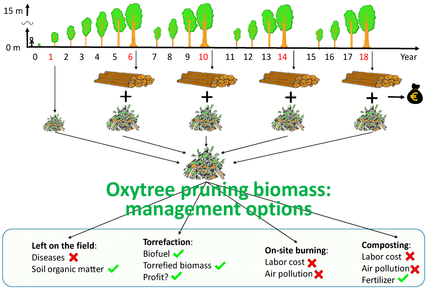
1. Introduction
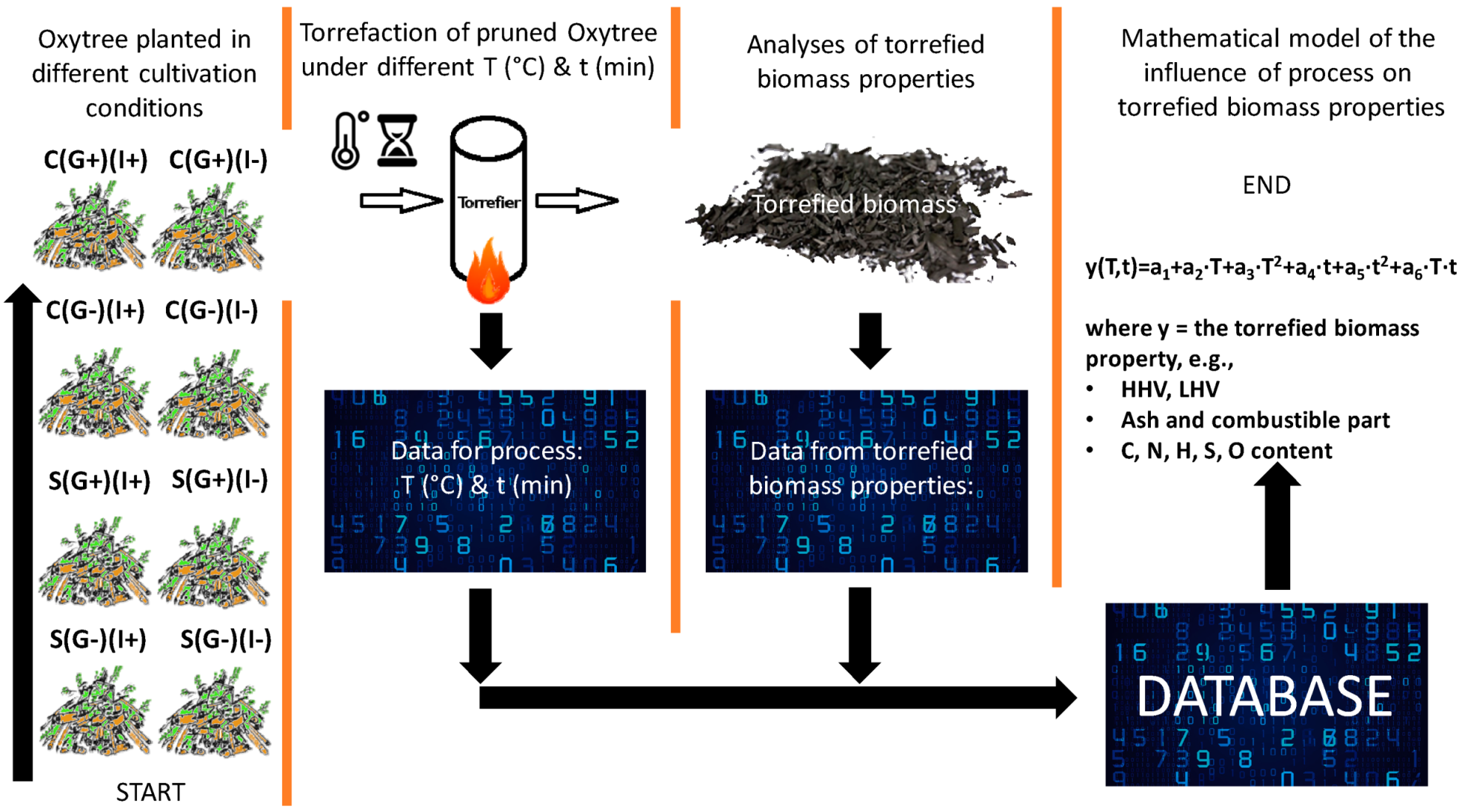
2. Materials and Methods
Models
3. Results
Models
- The first row contains a model to evaluate the particular properties of torrefied biomass and R2 value. AIC values are also presented in cases where an alternative model (e.g., model 2 or 3) was developed, and the data is presented in Appendix A;
- The first column shows the intercept a1 and coefficients a2–a6;
- The second column presents values for particular intercept/coefficients that are used in the model;
- The third column summarizes standard error calculated for particular intercept/coefficient.
- The fourth column presents p-values (probability value or significance). Statistical significance is assumed when p < 0.05).
- The fifth and sixth columns summarize the lower and upper limit of confidence of intercept/coefficient value.
- The seventh column summarizes the value of standardized regression coefficients (β) for each regression coefficients (a2–6).
- The name (model 1) in table description presents the original model . The alternative (model 2) and (model 3) stand for improved versions of a model without insignificant coefficients;
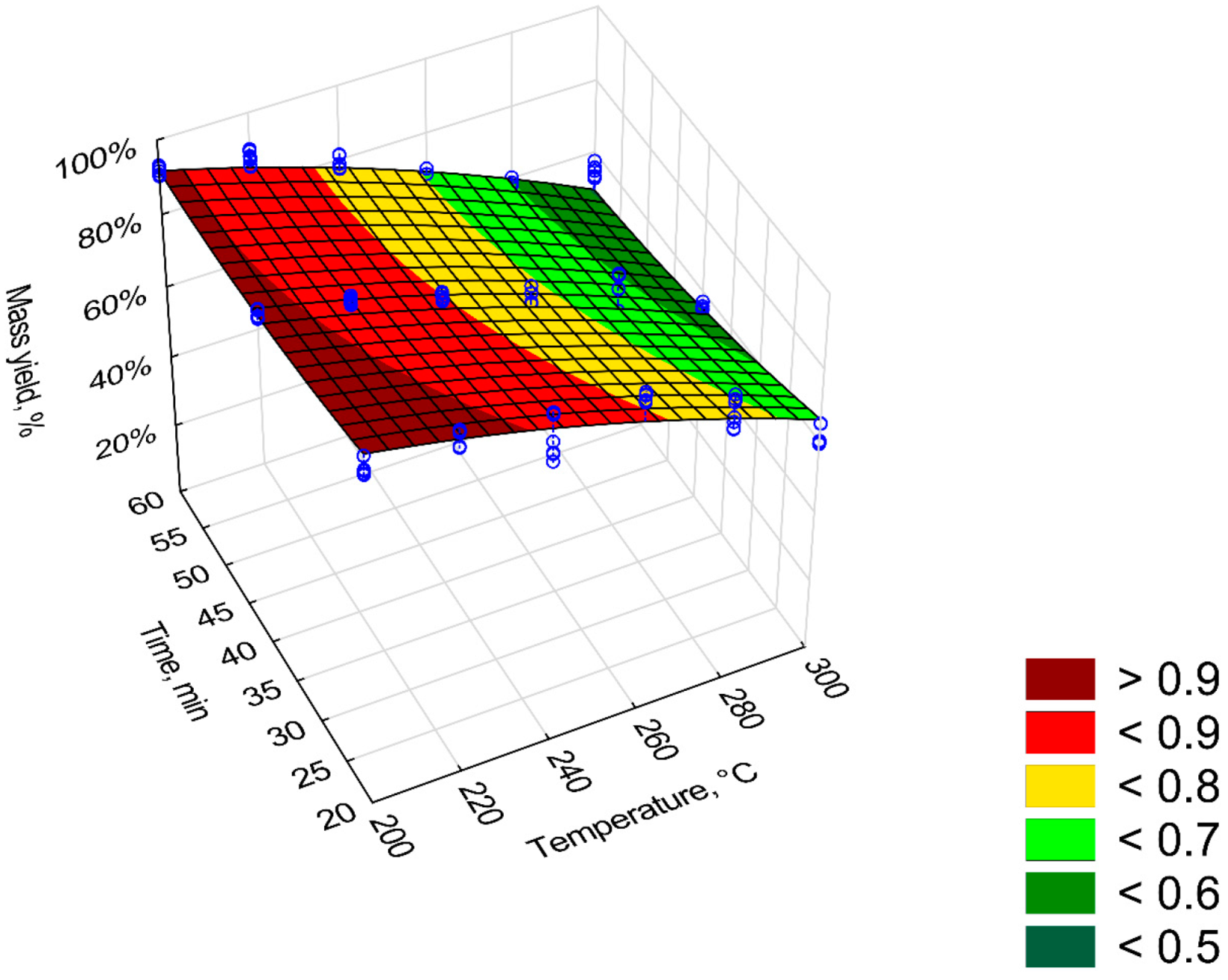
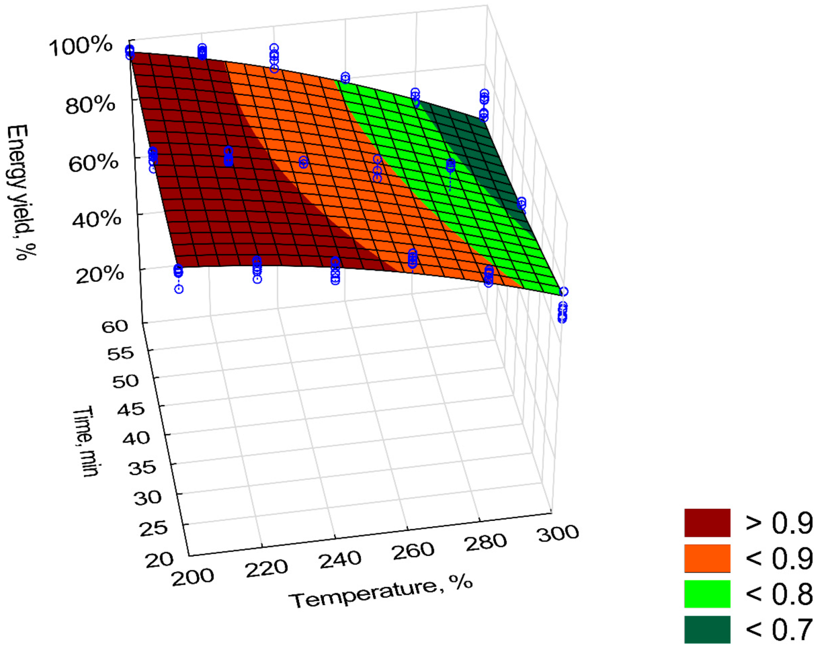
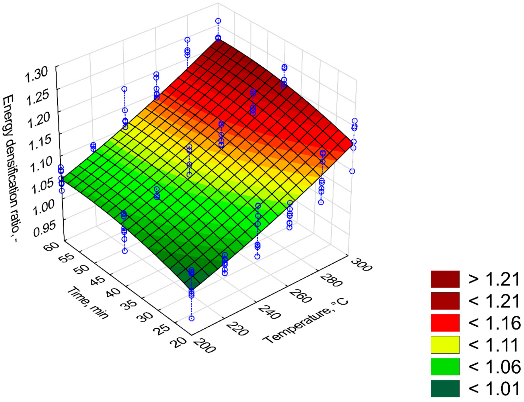
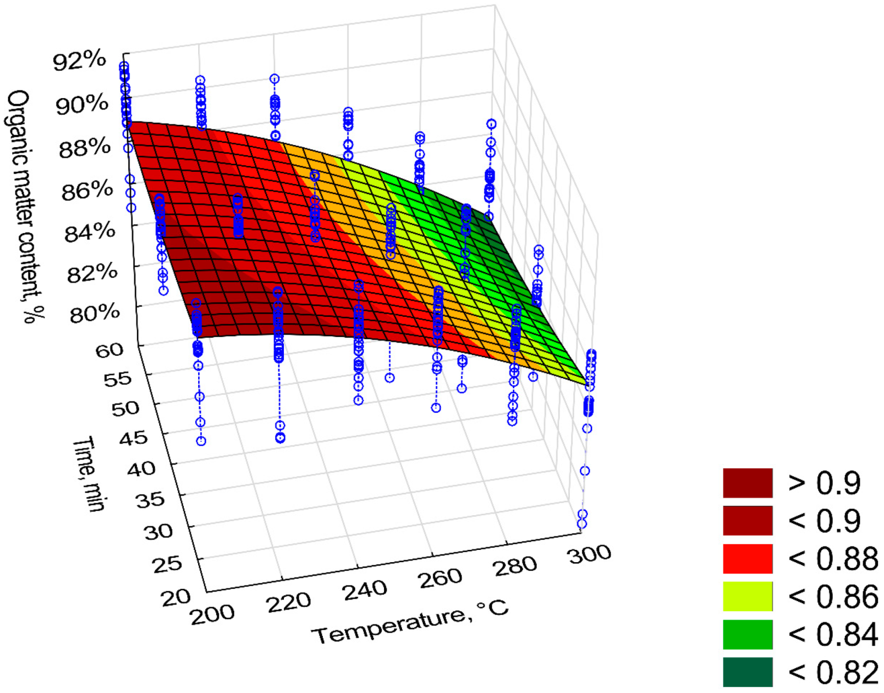
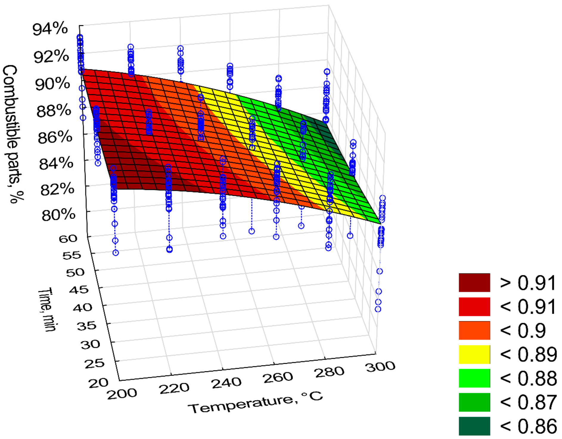
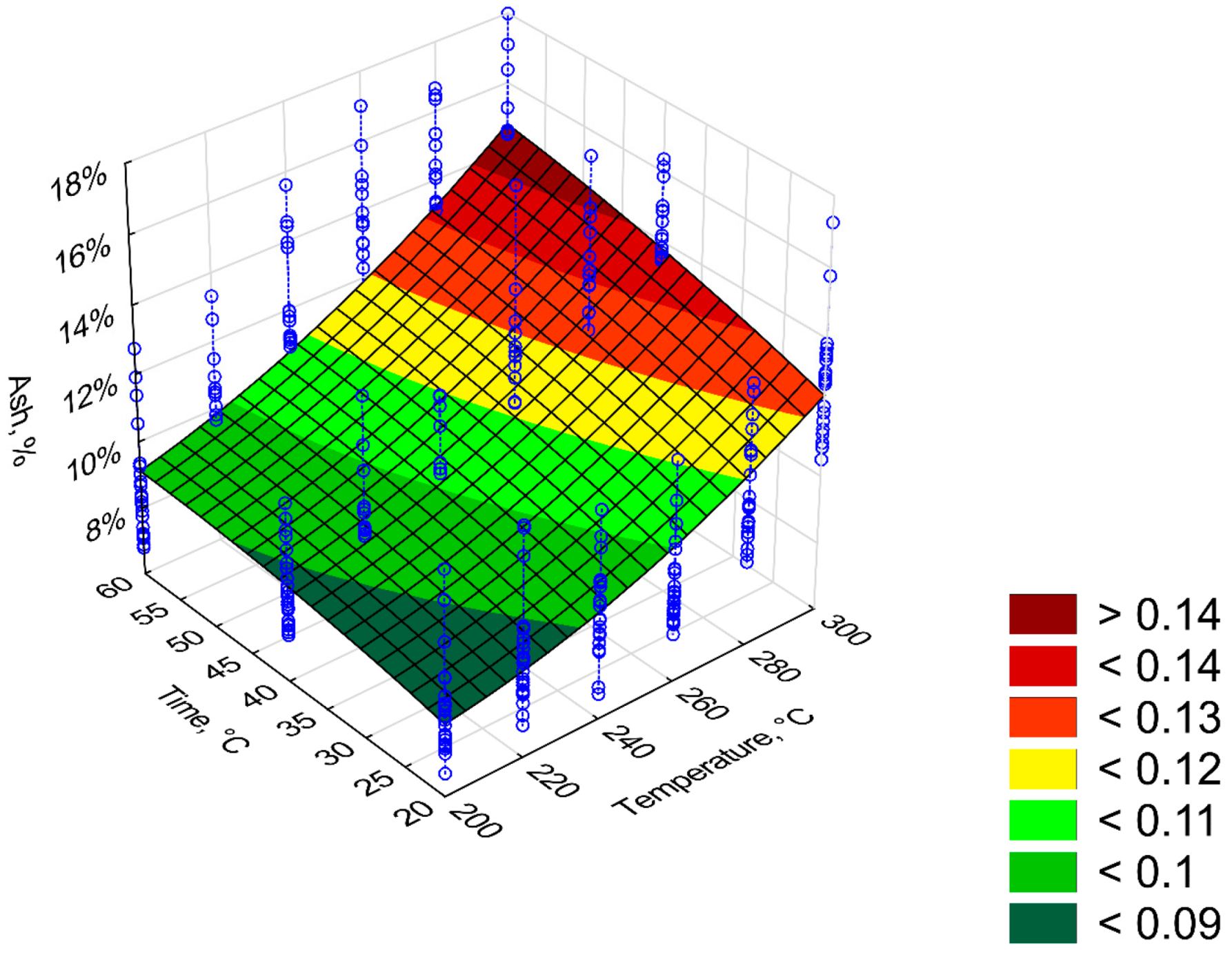
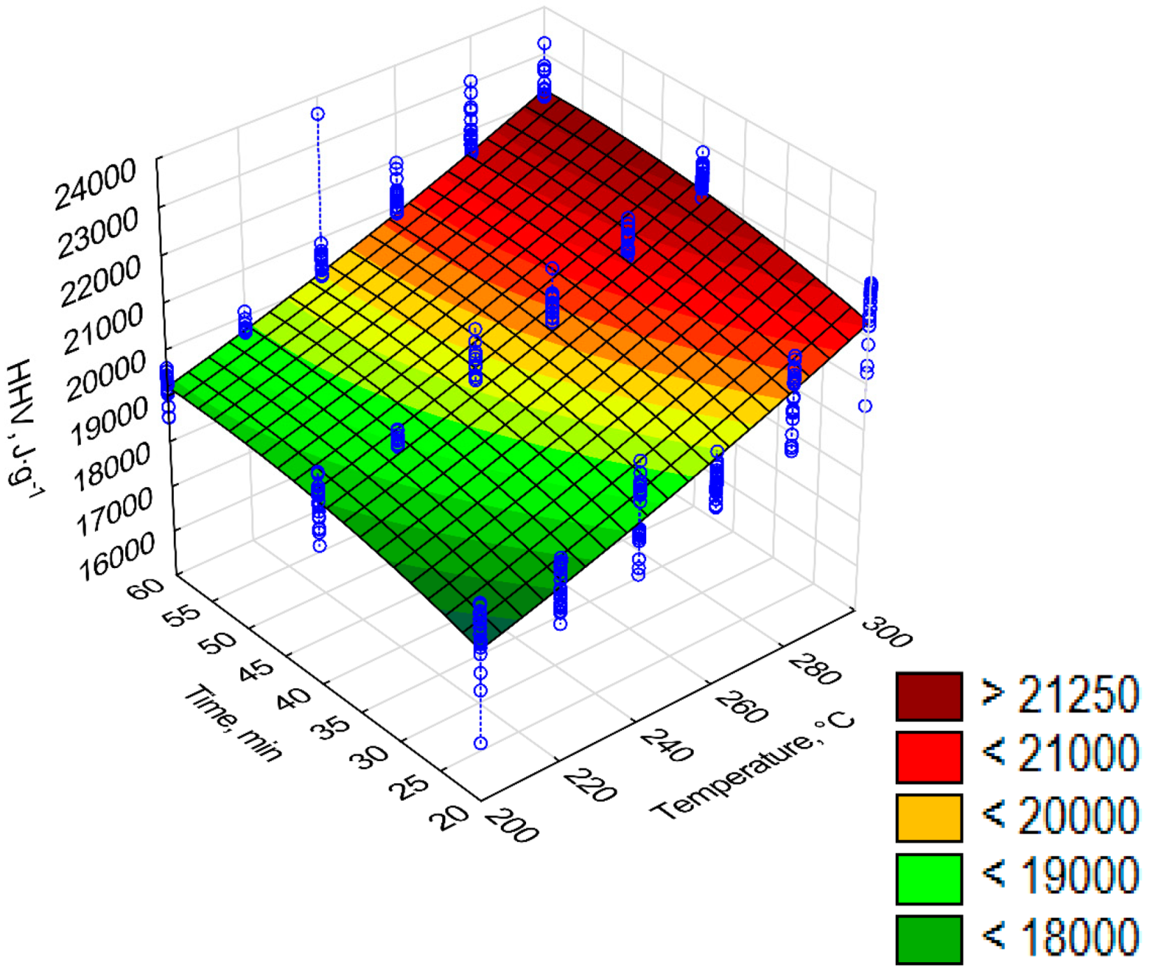
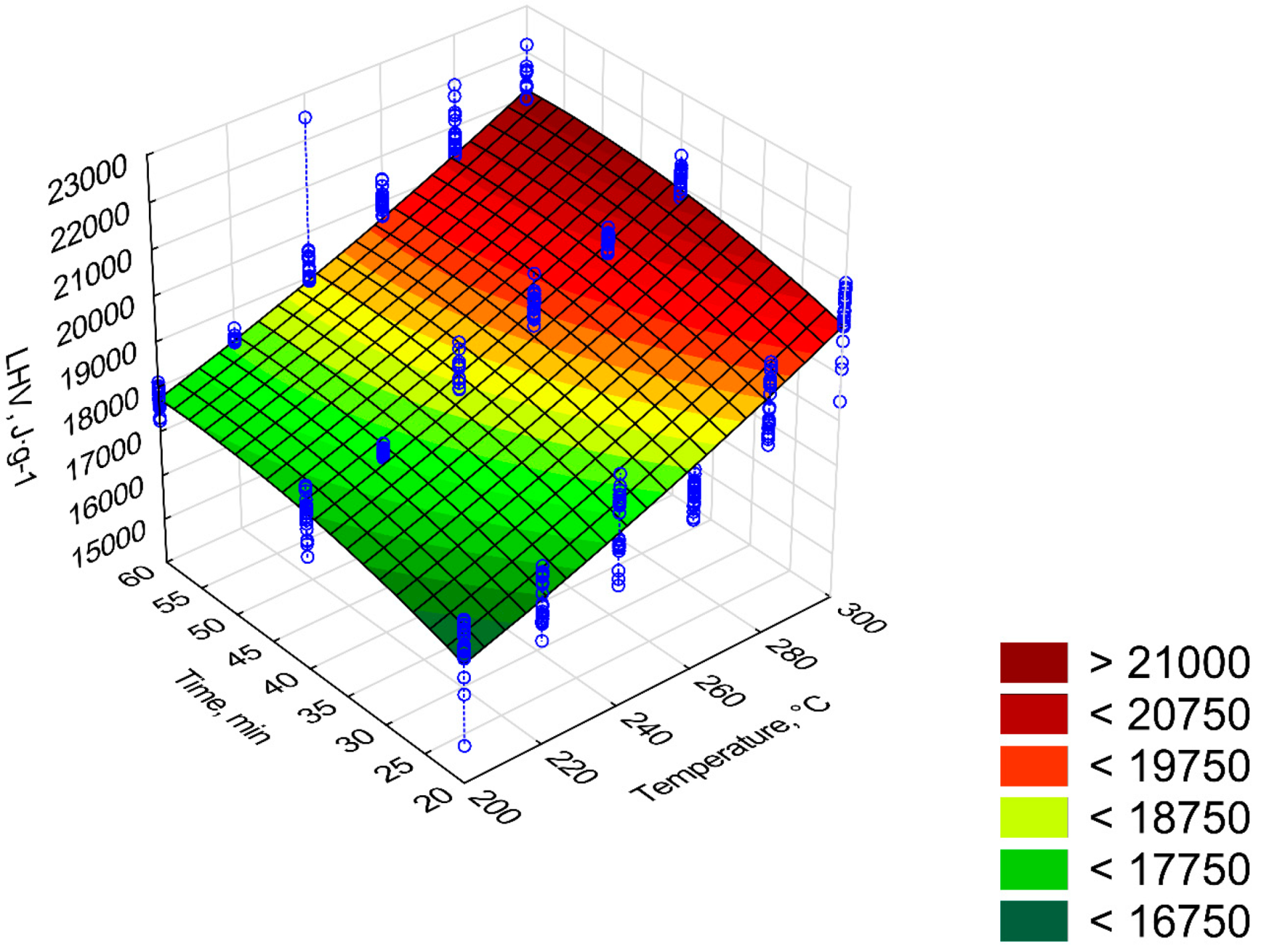
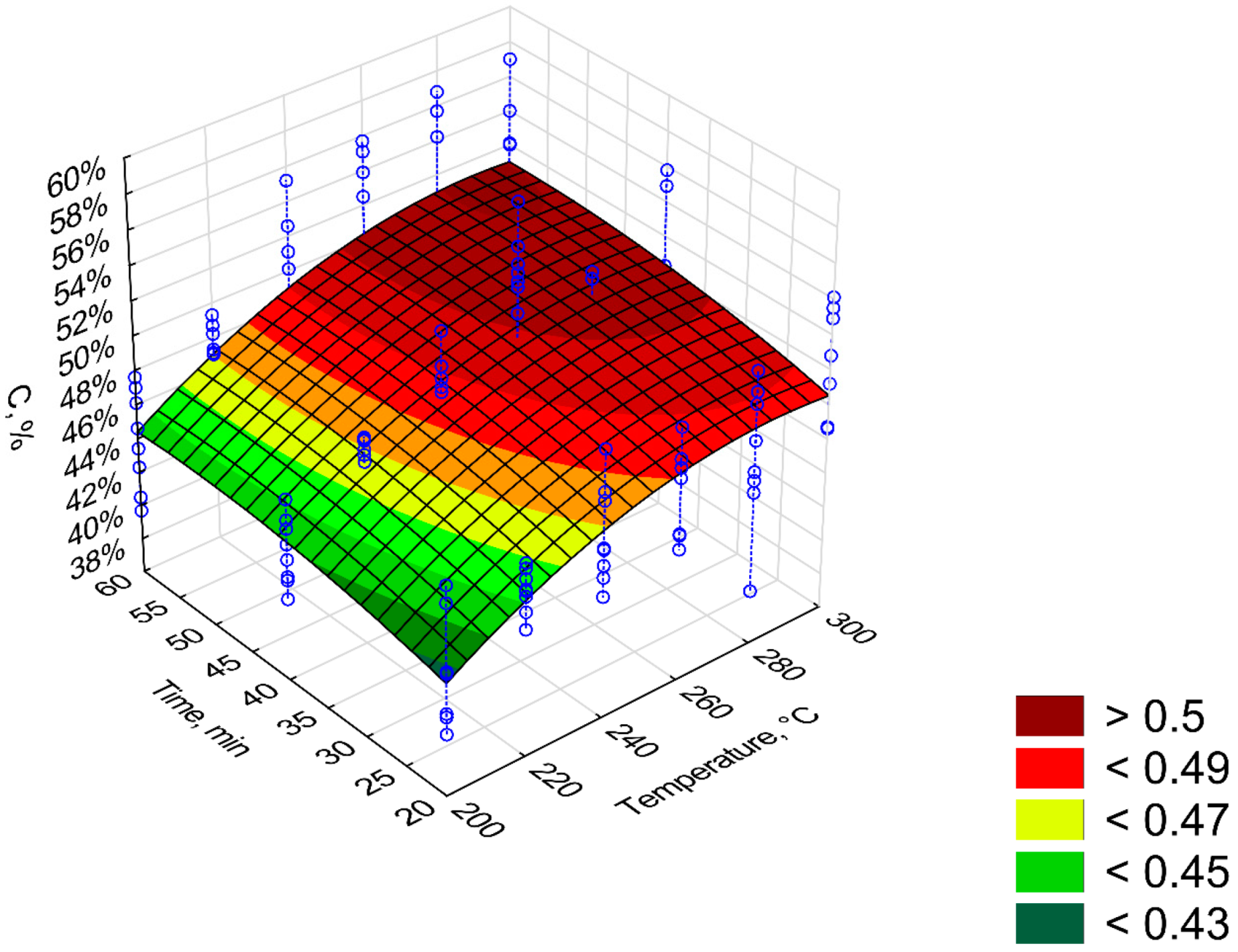
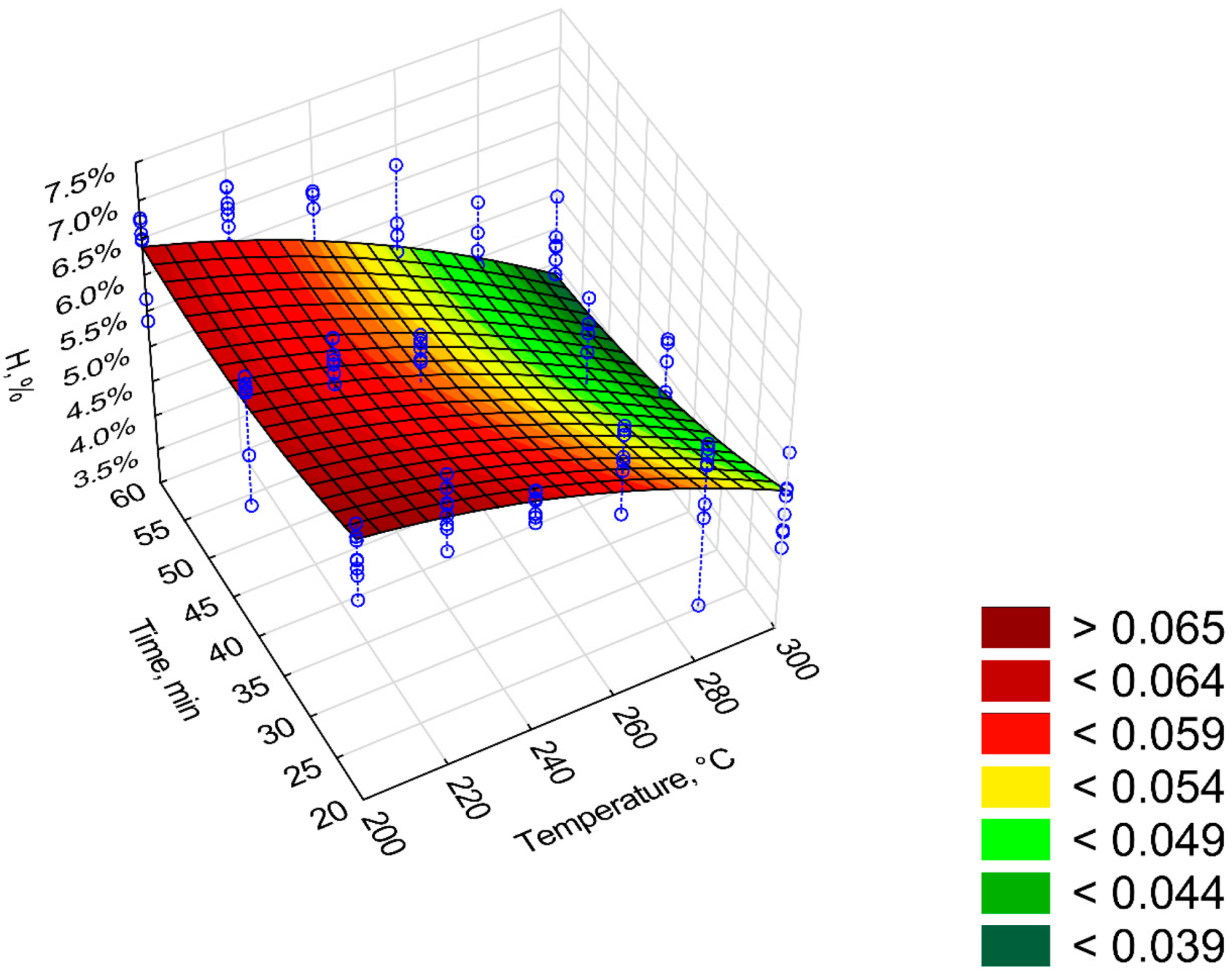
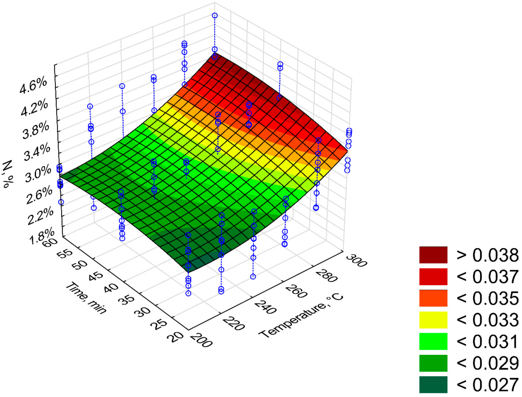
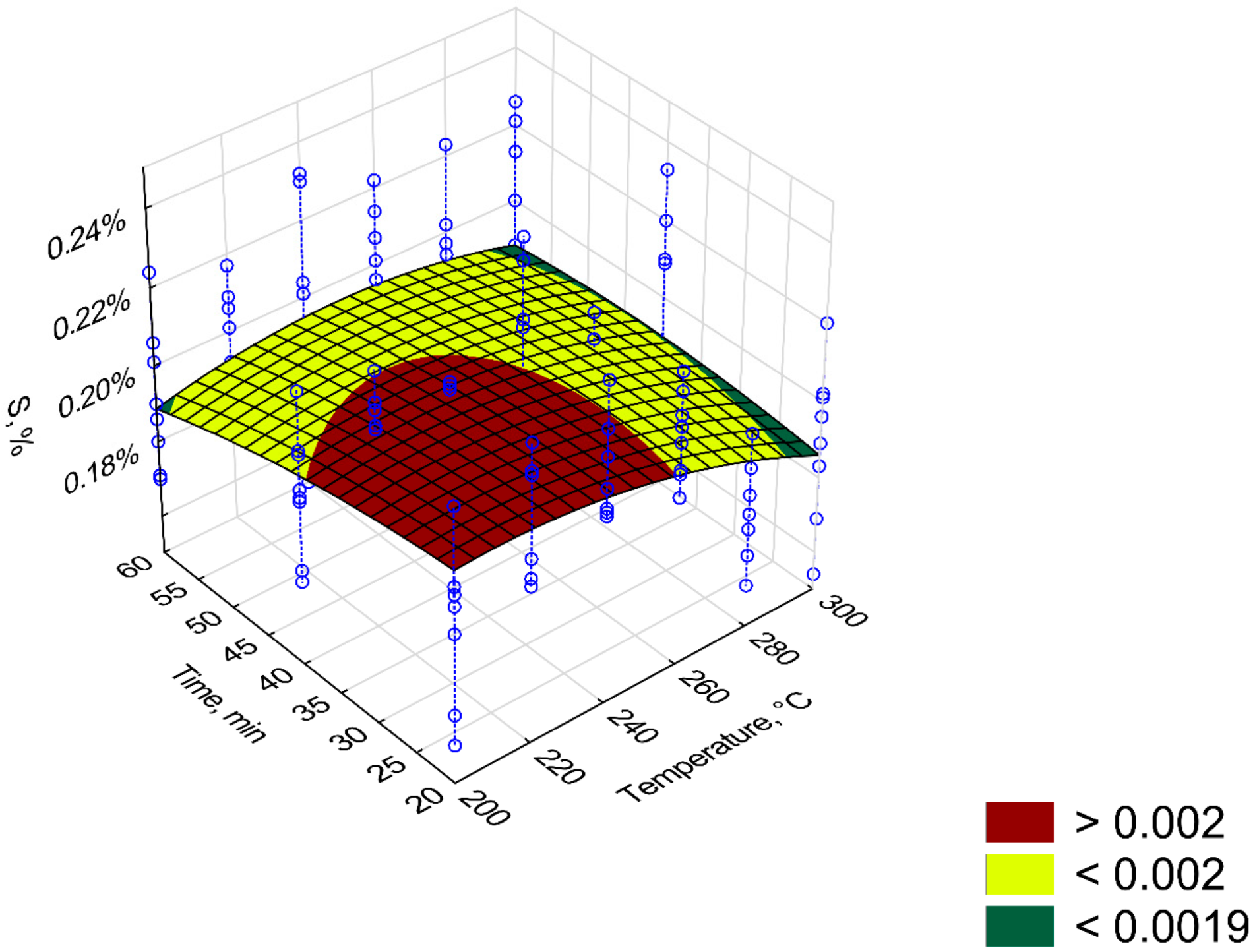
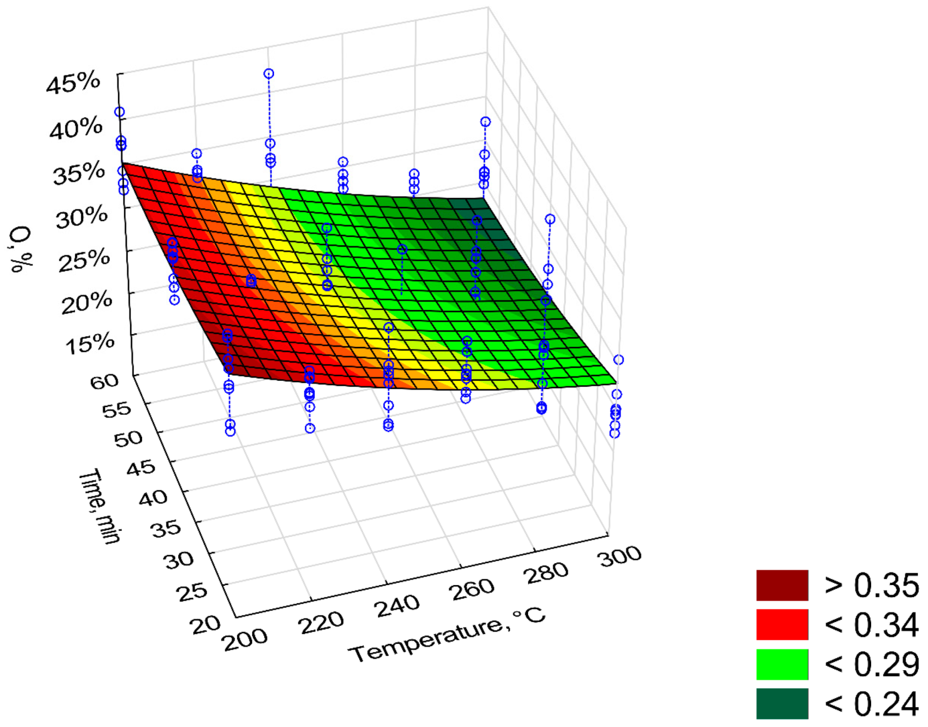
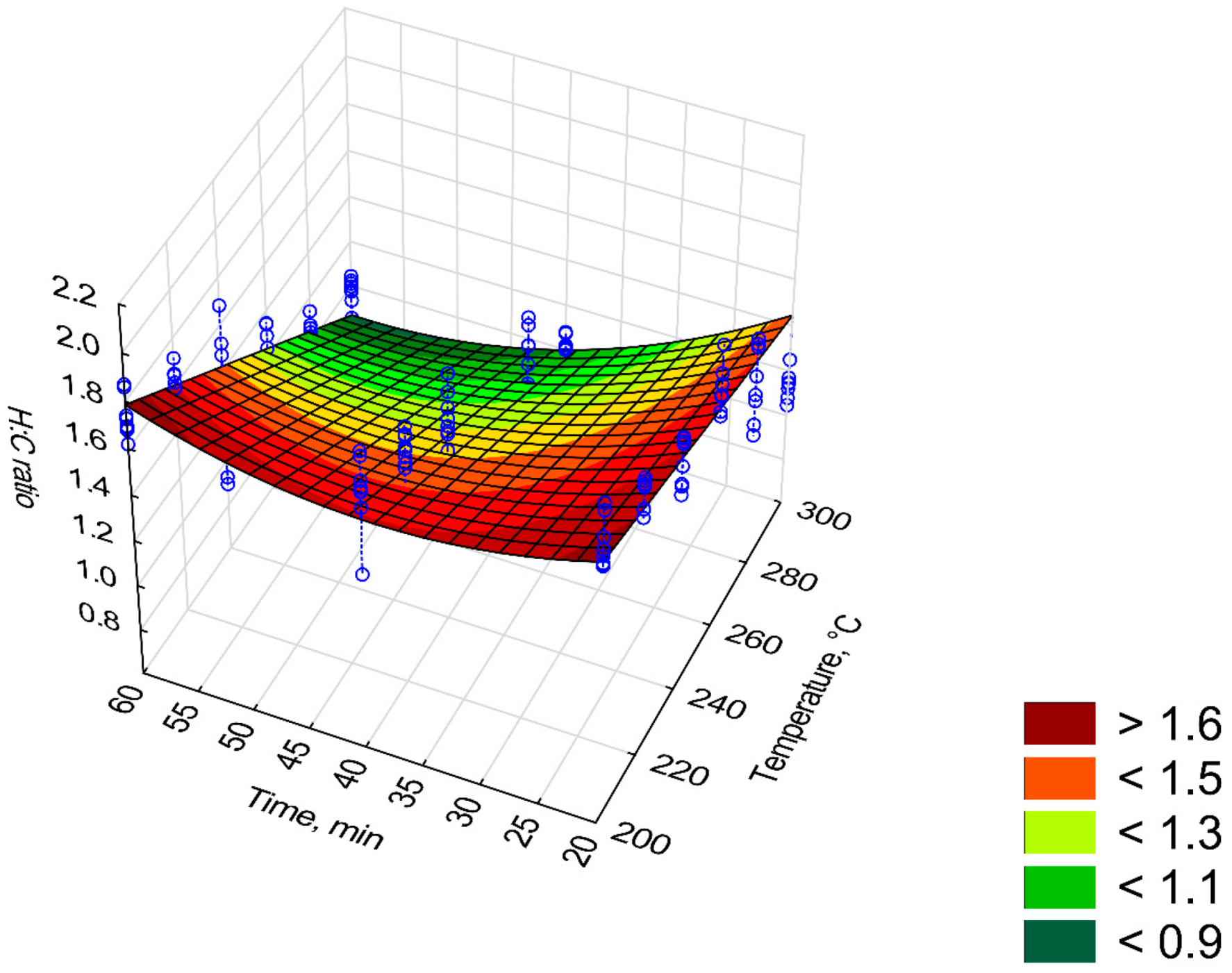
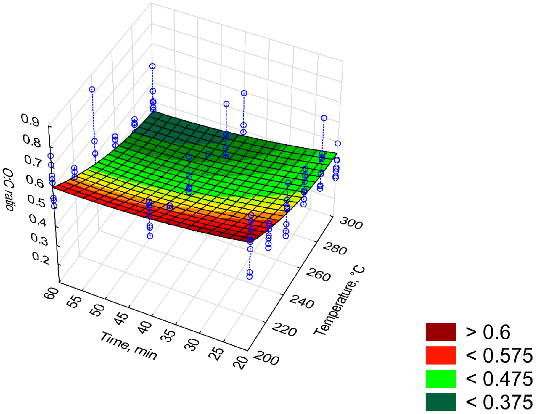
- Blue lines with circles present in figures stand for raw data used to nonlinear regression;
- Coefficients with (−) reduce the calculated value of y and coefficients with (+) increase the calculated value of y. The same system is used for standardized regression coefficients (β).
4. Discussion
4.1. Models
4.2. Evaluations of the Value of Torrefied Residue Biomass
- mass of Oxytree residues, Mg; assumed 1 Mg;
- the moisture content of Oxytree residues, %; assumed 50%;
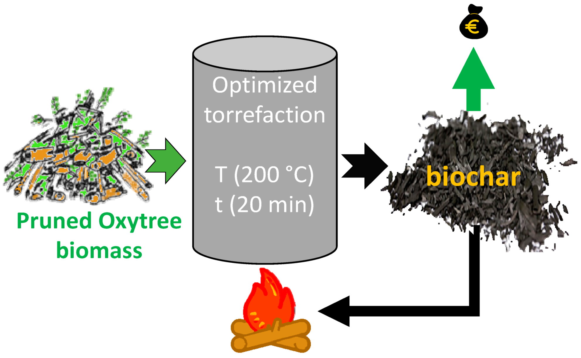
- torrefaction parameters temperature and time; assumed to be 200 °C and 20 min.
4.2.1. Initial Calculations
4.2.2. Main Properties of Torrefied Biomass Calculations
4.2.3. Energy Need to Torrefaction Process
4.2.4. Estimation of the Value of Torrefied Biomass
4.2.5. Profit from Torrefied Oxytree Residues
5. Conclusions
Supplementary Materials
Author Contributions
Funding
Conflicts of Interest
Appendix A

| Intercept/Coefficient | Value of Intercept/Coefficient | Standard Error | p | Lower Limit of Confidence | Upper Limit of Confidence | Standardized β Coefficient |
|---|---|---|---|---|---|---|
| a1 | 15,766.51 | 1816.820 | 8.67808 | 0.000000 | 12,195.46 | - |
| a2 | −6.93 | 14.197 | −0.48833 | 0.625567 | −34.84 | −0.19 |
| a3 | 0.07 | 0.028 | 2.46019 | 0.014282 | 0.01 | 0.94 |
| a4 | 60.04 | 17.365 | 3.45749 | 0.000600 | 25.91 | 0.78 |
| a5 | −0.67 | 0.148 | −4.50308 | 0.000009 | −0.96 | −0.70 |
| a6 | 0.07 | 0.050 | 1.33485 | 0.182637 | −0.03 | 0.23 |
| Intercept/Coefficient | Value of Intercept/Coefficient | Standard Error | p | Lower Limit of Confidence | Upper Limit of Confidence | Standardized β Coefficient |
|---|---|---|---|---|---|---|
| a1 | 14,913.84 | 1835.747 | 0.000000 | 11,305.59 | 18,522.09 | − |
| a2 | −16.21 | 14.345 | 0.259123 | −44.41 | 11.99 | −0.40 |
| a3 | 0.09 | 0.028 | 0.001152 | 0.04 | 0.15 | 1.14 |
| a4 | 64.87 | 17.546 | 0.000247 | 30.38 | 99.35 | 0.76 |
| a5 | −0.79 | 0.150 | 0.000000 | −1.09 | −0.50 | −0.75 |
| a6 | 0.10 | 0.051 | 0.042425 | 0.00 | 0.20 | 0.32 |
| Intercept/Coefficient | Value of Intercept/Coefficient | Standard Error | p | Lower Limit of Confidence | Upper Limit of Confidence | Standardized β Coefficient |
|---|---|---|---|---|---|---|
| a1 | 12,877.28 | 348.9176 | 0.000000 | 12,191.48 | 13,563.09 | − |
| a2 | 0.06 | 0.0043 | 0.000000 | 0.05 | 0.07 | 0.75 |
| a3 | 66.89 | 17.4595 | 0.000147 | 32.58 | 101.21 | 0.78 |
| a4 | −0.79 | 0.1501 | 0.000000 | −1.09 | −0.50 | −0.75 |
| a5 | 0.10 | 0.0502 | 0.058891 | 0.00 | 0.19 | 0.30 |
| Intercept/Coefficient | Value of Intercept/Coefficient | Standard Error | p | Lower Limit of Confidence | Upper Limit of Confidence | Standardized β Coefficient |
|---|---|---|---|---|---|---|
| a1 | 3.576069 | 0.780513 | 0.000010 | 2.032757 | 5.119380 | − |
| a2 | −0.007620 | 0.006099 | 0.213674 | −0.019680 | 0.004440 | −0.84 |
| a3 | 0.000004 | 0.000012 | 0.731624 | −0.000020 | 0.000028 | 0.23 |
| a4 | −0.011341 | 0.007460 | 0.130728 | −0.026092 | 0.003409 | −0.60 |
| a5 | 0.000200 | 0.000064 | 0.002132 | 0.000074 | 0.000326 | 0.85 |
| a6 | −0.000044 | 0.000022 | 0.041243 | −0.000087 | −0.000002 | −0.62 |
References
- Baležentis, T.; Streimikiene, D.; Zhang, T.; Liobikiene, G. The role of bioenergy in greenhouse gas emission reduction in EU countries: An Environmental Kuznets Curve modelling. Resour. Conserv. Recycl. 2019, 142, 225–231. [Google Scholar] [CrossRef]
- Paredes-Sánchez, J.P.; López-Ochoa, L.M.; López-González, L.M.; Las-Heras-Casas, J.; Xiberta-Bernat, J. Evolution and perspectives of the bioenergy applications in Spain. J. Clean. Prod. 2019, 213, 553–568. [Google Scholar] [CrossRef]
- Söderberg, C.; Eckerberg, K. Forest Policy and Economics Rising policy conflicts in Europe over bioenergy and forestry. For. Policy Econ. 2013, 33, 112–119. [Google Scholar] [CrossRef]
- Di Fulvio, F.; Forsell, N.; Korosuo, A.; Obersteiner, M.; Hellweg, S. Spatially explicit LCA analysis of biodiversity losses due to different bioenergy policies in the European Union. Sci. Total Environ. 2019, 651, 1505–1516. [Google Scholar] [CrossRef] [PubMed]
- Liszewski, M.; Bąbelewski, P. Oxytree plantation—Second year of research. Biomasa 2018, 8, 36–38. [Google Scholar]
- Jakubowski, M.; Tomczak, A.; Jelonek, T. The use of wood and the possibility of planting trees of the paulownia genus. Acta Sci. Pol. Silv. Colendar. Ratio Ind. Lignar. 2018, 17, 291–297. [Google Scholar] [CrossRef]
- Paulownia Bulletin ≠ 3. Advices And Instructions Paulownia For Biomass Production. Available online: http://paulowniatrees.eu/products/paulownia-planting-material (accessed on 10 March 2019).
- Hugo Durán Zuazo, V.; Antonio Jiménez Bocanegra, J.; Perea Torres, F.; Rodríguez Pleguezuelo, C.R.; Francia Martínez, J.R. Biomass Yield Potential of Paulownia Trees in a Semi-Arid Mediterranean Environment (S Spain). Int. J. Renew. Energy Res. 2013, 3. [Google Scholar]
- Dyjakon, A. The Influence of Apple Orchard Management on Energy Performance and Pruned Biomass Harvesting for Energetic Applications. Energies 2019, 12, 632. [Google Scholar] [CrossRef]
- Jabłoński, D. Oxytree: Wood for processing in a sawmill 6 years after planting. Available online: https://www.drewno.pl/artykuly/10535,oxytree-drewno-do-przerobu-w-tartaku-w-6-lat-od-posadzenia-drzewa.html (accessed on 12 March 2019).
- Basu, P. Biomass Gasification, Pyrolysis and Torrefaction, 2nd ed.; Academic Press: Cambridge, MA, USA, 2013; pp. 87–145. ISBN 978-0-12-396488-5. [Google Scholar]
- Chen, W.H.; Peng, J.; Bi, X.T. A state-of-the-art review of biomass torrfeaction, densification and applications. Renew. Susr. Energ. Rev. 2015, 44, 847–866. [Google Scholar] [CrossRef]
- Van der Stelt, M.J.C.; Gerhauser, H.; Kiel, J.H.A.; Ptasinski, K.J. Biomass upgrading by torrefaction for the production of biofuels: A review. Biomass Bioenergy 2011, 35, 3748–3762. [Google Scholar] [CrossRef]
- Jakubiak, M.; Kordylewski, W. Biomass torrefaction. Arch. Spalania 2010, 10, 11–25. [Google Scholar]
- Phanphanich, M.; Mani, S. Impact of torrefaction on the grindability and fuel characteristics of forest biomass. Biores. Technol. 2011, 102, 1246–1253. [Google Scholar] [CrossRef] [PubMed]
- Ahmed, N.; Rahmana, M.; Won, S.; Shim, S. Biochar properties and eco-friendly applications for climate change mitigation, waste management, and wastewater treatment: A review. Renew. Sust. Energy Rev. 2017, 79, 255–273. [Google Scholar] [CrossRef]
- Dudek, M.; Świechowski, K.; Manczarski, P.; Koziel, J.A.; Białowiec, A. The Effect of Biochar Addition on the Biogas Production Kinetics from the Anaerobic Digestion of Brewers’ Spent Grain. Energies 2019, 12, 1518. [Google Scholar] [CrossRef]
- Weber, K.; Quickerbhttps, P. Properties of biochar. Fuel 2018, 217, 240–261. [Google Scholar] [CrossRef]
- Świechowski, K.; Liszewski, M.; Bąbelewski, P.; Koziel, J.A.; Białowiec, A. Fuel Properties of Torrefied Biomass from Pruning of Oxytree. Data 2019, 4, 55. [Google Scholar] [CrossRef]
- Stegenta, S.; Kałdun, B.; Białowiec, A. Model selection and determination of kinetic parameters of respiratory activity of wastes during the aerobic process of biostabilization of municipal solid waste fraction. Rocz. Ochr. Środowiska 2016, 18, 800–814. [Google Scholar]
- Wang, L.; Barta-Rajnai, E.; Skreiberg, O.; Khalil, R.; Czégény, Z.; Jakab, E.; Barta, Z.; Grønli, M. Impact of Torrefaction on Woody Biomass Properties. Energy Procedia 2017, 105, 1149–1154. [Google Scholar] [CrossRef]
- Szymon, S.; Adrian, Ł.; Piersa, P.; Romanowska-Duda, Z.; Grzesik, M.; Cebula, A.; Kowalczyk, S. Renewable Energy Sources: Engineering, Technology, Innovation. Springer Int. Publ. AG 2018, 365–373. [Google Scholar] [CrossRef]
- Tumuluru, J.S.; Sokhansanj, S.; Hess, J.R.; Wright, C.T.; Boardman, R.D. A review on biomass torrefaction process and product properties for energy applications. Ind. Bioterchnol. 2011, 7, 373–384. [Google Scholar] [CrossRef]
- Wang, L.; Barta-Rajnai, E.; Skreiberg, Ø; Khalil, R.; Czégény, Z.; Jakab, E.; Barta, Z.; Grønli, M. Effect of torrefaction on physiochemical characteristics and grindability of stem wood, stump and bark. Appl. Energy 2018, 227, 137–148. [Google Scholar] [CrossRef]
- Pach, M.; Zanzi, R.; Bjornbom, E. Torrefied biomass a substitute for wood and charcoal. In Proceedings of the 6th Asia-Pacific International Symposium on Combustion and Energy Utilization, Kuala Lumpur, Malaysia, 20–22 May 2002. [Google Scholar]
- Khazraie Shoulaifar, T.; Demartini, N.; Zevenhoven, M.; Verhoeff, F.; Kiel, J.; Hupa, M. Ash-forming matter in torrefied birch wood: Changes in chemical association. Energy Fuels 2013, 27, 5684–5690. [Google Scholar] [CrossRef]
- Tumuluru, J.S. Comparison of Chemical Composition and Energy Property of Torrefied Switchgrass and Corn Stover. Front. Energy Res. 2015, 3, 1–11. [Google Scholar] [CrossRef]
- Grams, J.; Kwapińska, M.; Jędrzejczyk, M.; Rzeźnicka, I.; Leahy, J.J.; Ruppert, A.M. Surface characterization of Miscanthus × giganteus and Willow subjected to torrefaction. J. Anal. Appl. Pyrolysis 2019, 138, 231–241. [Google Scholar] [CrossRef]
- Rodrigues, A.; Loureiro, L.; Nunes, L.J.R. Torrefaction of woody biomasses from poplar SRC and Portuguese roundwood: Properties of torrefied products. Biomass Bioenergy 2018, 108, 55–65. [Google Scholar] [CrossRef]
- Li, S.; Harris, S.; Anandhi, A.; Chen, G. Predicting biochar properties and functions based on feedstock and pyrolysis temperature: A review and data syntheses. J. Clean. Prod. 2019, 215, 890–902. [Google Scholar] [CrossRef]
- Lu, J.J.; Chen, W.H. Product yields and characteristics of corncob waste under various torrefaction atmospheres. Energies 2014, 7, 13–27. [Google Scholar] [CrossRef]
- Ren, X.; Sun, R.; Meng, X.; Vorobiev, N.; Schiemann, M.; Levendis, Y.A. Carbon, sulfur and nitrogen oxide emissions from combustion of pulverized raw and torrefied biomass. Fuel 2017, 188, 310–323. [Google Scholar] [CrossRef]
- Li, S.; Chen, G. Thermogravimetric, thermochemical, and infrared spectral characterization of feedstocks and biochar derived at different pyrolysis temperatures. Waste Manag. 2018, 78, 198–207. [Google Scholar] [CrossRef]
- Li, S.; Barreto, V.; Li, R.; Chen, G.; Hsieh, Y.P. Nitrogen retention of biochar derived from different feedstocks at variable pyrolysis temperatures. J. Anal. Appl. Pyrolysis 2018, 133, 136–146. [Google Scholar] [CrossRef]
- Novak, J.; Lima, I.; Xing, B.; Gaskin, J.W.; Steiner, C.; Das, K.C.; Ahmedna, M.; Rehrah, D.; Watts, D.W.; Busscher, W.J.; et al. Characterization of designer biochar produced at different temperatures and their effects on a loamy sand. Ann. Environ. Sci. 2009, 3, 195–206. [Google Scholar]
- Akanni, A.A.; Kolawole, O.J.; Dayanand, P.; Ajani, L.O.; Madhurai, M. Influence of torrefaction on lignocellulosic woody biomass of Nigerian origin. J. Chem. Technol. Metall. 2019, 54, 274–285. [Google Scholar]
- Markič, M.; Kalan, Z.; Pezdič, J.; Faganeli, J. H/C versus O/C atomic ratio characterization of selected coals in Slovenia. Geologija 2011, 50, 403–426. [Google Scholar] [CrossRef]
- Stępień, P.; Mysior, M.; Bialowiec, A. Technical and techn ological problems and aplicability of waste torrefaction. In Innovations in Waste Management. Selected Issues; Białowiec, A., Ed.; Wydawnictwo Uniwersytetu Przyrodniczego we Wrocławiu: Wrocław, Dolnośląskie, 2018; ISBN 9788377172780. [Google Scholar] [CrossRef]
- Brusseau, M.L.; Walker, D.B.; Fitzsimmons, K. Physical-Chemical Characteristics of Water, 3rd ed.; Elsevier Inc.: Amsterdam, The Netherlands, 2019; ISBN 9780128147191. [Google Scholar]
- Radmanović, K.; Đukić, I.; Pervan, S. Specific Heat Capacity of Wood. Drv. Ind. 2014, 65, 151–157. [Google Scholar] [CrossRef]
- Portal Gospodarczy, Coal Prices. Available online: https://www.wnp.pl/gornictwo/notowania/ceny_wegla_pgg/ (accessed on 12 March 2019).


| Intercept/Coefficient | Value of Intercept/Coefficient | Standard Error | p | Lower Limit of Confidence | Upper Limit of Confidence | Standardized β Coefficient |
|---|---|---|---|---|---|---|
| a1 | 0.891816 | 0.223378 | 0.000000 | 0.450129 | 1.333503 | – |
| a2 | 0.003525 | 0.001746 | 0.000000 | 0.000074 | 0.006977 | 0.83 |
| a3 | −0.000013 | 0.000000 | 0.000000 | −0.000013 | −0.000013 | −1.49 |
| a4 | −0.001684 | 0.002135 | 0.000000 | −0.005905 | 0.002538 | −0.19 |
| a5 | 0.000062 | 0.000018 | 0.000000 | 0.000025 | 0.000098 | 0.56 |
| a6 | −0.000025 | 0.000000 | 0.000000 | −0.000025 | −0.000025 | −0.74 |
| Intercept/Coefficient | Value of Intercept/Coefficient | Standard Error | p | Lower Limit of Confidence | Upper Limit of Confidence | Standardized β Coefficient |
|---|---|---|---|---|---|---|
| a1 | 0.429884 | 0.219439 | 0.000000 | −0.004012 | 0.863781 | – |
| a2 | 0.006285 | 0.001715 | 0.000000 | 0.002894 | 0.009675 | 1.85 |
| a3 | −0.000016 | 0.000000 | 0.000000 | −0.000016 | −0.000016 | −2.35 |
| a4 | 0.002472 | 0.002097 | 0.000000 | −0.001675 | 0.006619 | 0.35 |
| a5 | 0.000037 | 0.000018 | 0.000000 | 0.000002 | 0.000073 | 0.42 |
| a6 | −0.000031 | 0.000000 | 0.000000 | −0.000031 | −0.000031 | −1.16 |
| Intercept/Coefficient | Value of Intercept/Coefficient | Standard Error | p | Lower Limit of Confidence | Upper Limit of Confidence | Standardized β Coefficient |
|---|---|---|---|---|---|---|
| a1 | 0.860189 | 0.182285 | 0.000000 | 0.499756 | 1.220621 | – |
| a2 | −0.000366 | 0.001424 | 0.000000 | −0.003183 | 0.002450 | −0.18 |
| a3 | 0.000004 | 0.000000 | 0.000000 | 0.000004 | 0.000004 | 0.93 |
| a4 | 0.003294 | 0.001742 | 0.000000 | −0.000151 | 0.006739 | 0.78 |
| a5 | −0.000037 | 0.000015 | 0.000000 | −0.000066 | −0.000007 | −0.70 |
| a6 | 0.000004 | 0.000000 | 0.000000 | 0.000004 | 0.000004 | 0.23 |
| Intercept/Coefficient | Value of Intercept/Coefficient | Standard Error | p | Lower Limit of Confidence | Upper Limit of Confidence | Standardized β Coefficient |
|---|---|---|---|---|---|---|
| a1 | 0.764595 | 0.059289 | 0.000000 | 0.648061 | 0.881130 | – |
| a2 | 0.001510 | 0.000463 | 0.000000 | 0.000600 | 0.002421 | 1.76 |
| a3 | −0.000004 | 0.000000 | 0.000000 | −0.000004 | −0.000004 | −2.21 |
| a4 | 0.000138 | 0.000567 | 0.000000 | −0.000976 | 0.001252 | 0.08 |
| a5 | 0.000008 | 0.000000 | 0.000000 | 0.000008 | 0.000008 | 0.35 |
| a6 | −0.000005 | 0.000000 | 0.000000 | −0.000005 | −0.000005 | −0.76 |
| Intercept/Coefficient | Value of Intercept/Coefficient | Standard Error | p | Lower Limit of Confidence | Upper Limit of Confidence | Standardized β Coefficient |
|---|---|---|---|---|---|---|
| a1 | 0.838668 | 0.054980 | 0.000000 | 0.730603 | 0.946733 | – |
| a2 | 0.000997 | 0.000430 | 0.000000 | 0.000152 | 0.001841 | 1.33 |
| a3 | −0.000003 | 0.000000 | 0.000000 | −0.000003 | −0.000003 | −1.81 |
| a4 | 0.000029 | 0.000526 | 0.000000 | −0.001004 | 0.001062 | 0.02 |
| a5 | 0.000005 | 0.000000 | 0.000000 | 0.000005 | 0.000005 | 0.28 |
| a6 | −0.000004 | 0.000000 | 0.000000 | −0.000004 | −0.000004 | −0.60 |
| Intercept/Coefficient | Value of Intercept/Coefficient | Standard Error | p | Lower Limit of Confidence | Upper Limit of Confidence | Standardized β Coefficient |
|---|---|---|---|---|---|---|
| a1 | 0.161333 | 0.054979 | 0.000000 | 0.053268 | 0.269398 | – |
| a2 | −0.000997 | 0.000430 | 0.000000 | −0.001841 | −0.000152 | −1.33 |
| a3 | 0.000003 | 0.000000 | 0.000000 | 0.000003 | 0.000003 | 1.81 |
| a4 | −0.000029 | 0.000525 | 0.000000 | −0.001062 | 0.001004 | −0.02 |
| a5 | −0.000005 | 0.000000 | 0.000000 | −0.000005 | −0.000005 | −0.28 |
| a6 | 0.000004 | 0.000000 | 0.000000 | 0.000004 | 0.000004 | 0.60 |
| Intercept/Coefficient | Value of Intercept/Coefficient | Standard Error | p | Lower Limit of Confidence | Upper Limit of Confidence | Standardized β Coefficient |
|---|---|---|---|---|---|---|
| a1 | 14,572.93 | 235.6392 | 0.000000 | 14109.78 | 15,036.09 | – |
| a2 | 0.06 | 0.0016 | 0.000000 | 0.06 | 0.06 | 0.83 |
| a3 | 76.79 | 12.0003 | 0.000000 | 53.20 | 100.38 | 1.00 |
| a4 | −0.67 | 0.1485 | 0.000009 | −0.96 | −0.38 | −0.70 |
| Intercept/Coefficient | Value of Intercept/Coefficient | Standard Error | p | Lower Limit of Confidence | Upper Limit of Confidence | Standardized β Coefficient |
|---|---|---|---|---|---|---|
| a1 | 12,394.39 | 238.9256 | 0.000000 | 11,924.77 | 12,864.00 | – |
| a2 | 0.07 | 0.0017 | 0.000000 | 0.07 | 0.07 | 0.84 |
| a3 | 90.68 | 12.1676 | 0.000000 | 66.76 | 114.59 | 1.06 |
| a4 | −0.79 | 0.1505 | 0.000000 | −1.09 | −0.50 | −0.75 |
| Intercept/Coefficient | Value of Intercept/Coefficient | Standard Error | p | Lower Limit of Confidence | Upper Limit of Confidence | Standardized β Coefficient |
|---|---|---|---|---|---|---|
| a1 | −0.212855 | 0.188451 | 0.000000 | −0.585480 | 0.159770 | − |
| a2 | 0.004700 | 0.001473 | 0.000000 | 0.001788 | 0.007612 | 3.80 |
| a3 | −0.000008 | 0.000000 | 0.000000 | −0.000008 | −0.000008 | −3.35 |
| a4 | 0.001477 | 0.001801 | 0.000000 | −0.002084 | 0.005039 | 0.57 |
| a5 | −0.000017 | 0.000015 | 0.000000 | −0.000047 | 0.000014 | −0.52 |
| a6 | 0.000002 | 0.000000 | 0.000000 | 0.000002 | 0.000002 | 0.16 |
| Intercept/Coefficient | Value of Intercept/Coefficient | Standard Error | p | Lower Limit of Confidence | Upper Limit of Confidence | Standardized β Coefficient |
|---|---|---|---|---|---|---|
| a1 | 0.042265 | 0.032430 | 0.000000 | −0.021858 | 0.106388 | − |
| a2 | 0.000377 | 0.000253 | 0.000000 | −0.000124 | 0.000878 | 1.27 |
| a3 | −0.000001 | 0.000000 | 0.000000 | −0.000001 | −0.000001 | −1.74 |
| a4 | −0.000164 | 0.000310 | 0.000000 | −0.000777 | 0.000449 | −0.27 |
| a5 | 0.000006 | 0.000000 | 0.000000 | 0.000006 | 0.000006 | 0.75 |
| a6 | −0.000002 | 0.000000 | 0.000000 | −0.000002 | −0.000002 | −0.85 |
| Intercept/Coefficient | Value of Intercept/Coefficient | Standard Error | p | Lower Limit of Confidence | Upper Limit of Confidence | Standardized β Coefficient |
|---|---|---|---|---|---|---|
| a1 | 0.068473 | 0.023985 | 0.000000 | 0.021047 | 0.115899 | − |
| a2 | −0.000429 | 0.000187 | 0.000000 | −0.000800 | −0.000059 | −2.59 |
| a3 | 0.000001 | 0.000000 | 0.000000 | 0.000001 | 0.000001 | 3.01 |
| a4 | 0.000134 | 0.000229 | 0.000000 | −0.000319 | 0.000588 | 0.39 |
| a5 | −0.000003 | 0.000000 | 0.000000 | −0.000003 | −0.000003 | −0.71 |
| a6 | 0.000001 | 0.000000 | 0.000000 | 0.000001 | 0.000001 | 0.51 |
| Intercept/Coefficient | Value of Intercept/Coefficient | Standard Error | p | Lower Limit of Confidence | Upper Limit of Confidence | Standardized β Coefficient |
|---|---|---|---|---|---|---|
| a1 | 0.001055 | 0.001325 | 0.000000 | −0.001566 | 0.003676 | − |
| a2 | 0.000010 | 0.000010 | 0.000000 | −0.000010 | 0.000031 | 1.41 |
| a3 | 2.61 × 10⁻⁸ | 0.000000 | 0.000000 | 0.000000 | 0.000000 | −1.81 |
| a4 | −0.000008 | 0.000013 | 0.000000 | −0.000033 | 0.000017 | −0.52 |
| a5 | 6.77 × 10⁻⁸ | 0.000000 | 0.000000 | 0.000000 | 0.000000 | −0.36 |
| a6 | 4.63 × 10⁻⁸ | 0.000000 | 0.000000 | 0.000000 | 0.000000 | 0.81 |
| Intercept/Coefficient | Value of Intercept/Coefficient | Standard Error | p | Lower Limit of Confidence | Upper Limit of Confidence | Standardized β Coefficient |
|---|---|---|---|---|---|---|
| a1 | 0.873544 | 0.207078 | 0.000000 | 0.464088 | 1.283001 | − |
| a2 | −0.003199 | 0.001618 | 0.000000 | −0.006398 | 0.000001 | −1.96 |
| a3 | 0.000005 | 0.000000 | 0.000000 | 0.000005 | 0.000005 | 1.42 |
| a4 | −0.001367 | 0.001979 | 0.000000 | −0.005280 | 0.002547 | −0.40 |
| a5 | 0.000022 | 0.000017 | 0.000000 | −0.000011 | 0.000055 | 0.52 |
| a6 | −0.000005 | 0.000000 | 0.000000 | −0.000005 | −0.000005 | −0.41 |
| Intercept/Coefficient | Value of Intercept/Coefficient | Standard Error | p | Lower Limit of Confidence | Upper Limit of Confidence | Standardized β Coefficient |
|---|---|---|---|---|---|---|
| a1 | 2.207455 | 0.044156 | 0.000000 | 2.120162 | 2.294748 | − |
| a2 | 0.000394 | 0.000029 | 0.000000 | 0.000338 | 0.000451 | 1.68 |
| a3 | −0.000153 | 0.000000 | 0.000000 | −0.000153 | −0.000153 | −2.15 |
| Intercept/Coefficient | Value of Intercept/Coefficient | Standard Error | p | Lower Limit of Confidence | Upper Limit of Confidence | Standardized β Coefficient |
|---|---|---|---|---|---|---|
| a1 | 0.022935 | 0.005095 | 0.000000 | 0.012860 | 0.033010 | - |
| a2 | −0.000114 | 0.000040 | 0.000000 | −0.000192 | −0.000035 | −3.03 |
| a3 | 1.85 × 10⁻⁵ | 0.000000 | 0.000000 | 0.000000 | 0.000000 | 2.47 |
| a4 | −0.000047 | 0.000049 | 0.000000 | −0.000143 | 0.000050 | −0.59 |
| a5 | 5.38 × 10⁻⁵ | 0.000000 | 0.000000 | 0.000001 | 0.000001 | 0.55 |
| a6 | −6.26 × 10⁻⁵ | 0.000000 | 0.000000 | 0.000000 | 0.000000 | −0.21 |
© 2019 by the authors. Licensee MDPI, Basel, Switzerland. This article is an open access article distributed under the terms and conditions of the Creative Commons Attribution (CC BY) license (http://creativecommons.org/licenses/by/4.0/).
Share and Cite
Świechowski, K.; Liszewski, M.; Bąbelewski, P.; Koziel, J.A.; Białowiec, A. Oxytree Pruned Biomass Torrefaction: Mathematical Models of the Influence of Temperature and Residence Time on Fuel Properties Improvement. Materials 2019, 12, 2228. https://doi.org/10.3390/ma12142228
Świechowski K, Liszewski M, Bąbelewski P, Koziel JA, Białowiec A. Oxytree Pruned Biomass Torrefaction: Mathematical Models of the Influence of Temperature and Residence Time on Fuel Properties Improvement. Materials. 2019; 12(14):2228. https://doi.org/10.3390/ma12142228
Chicago/Turabian StyleŚwiechowski, Kacper, Marek Liszewski, Przemysław Bąbelewski, Jacek A. Koziel, and Andrzej Białowiec. 2019. "Oxytree Pruned Biomass Torrefaction: Mathematical Models of the Influence of Temperature and Residence Time on Fuel Properties Improvement" Materials 12, no. 14: 2228. https://doi.org/10.3390/ma12142228
APA StyleŚwiechowski, K., Liszewski, M., Bąbelewski, P., Koziel, J. A., & Białowiec, A. (2019). Oxytree Pruned Biomass Torrefaction: Mathematical Models of the Influence of Temperature and Residence Time on Fuel Properties Improvement. Materials, 12(14), 2228. https://doi.org/10.3390/ma12142228