Health Degradation Monitoring and Early Fault Diagnosis of a Rolling Bearing Based on CEEMDAN and Improved MMSE


Abstract
1. Introduction
2. Methodology
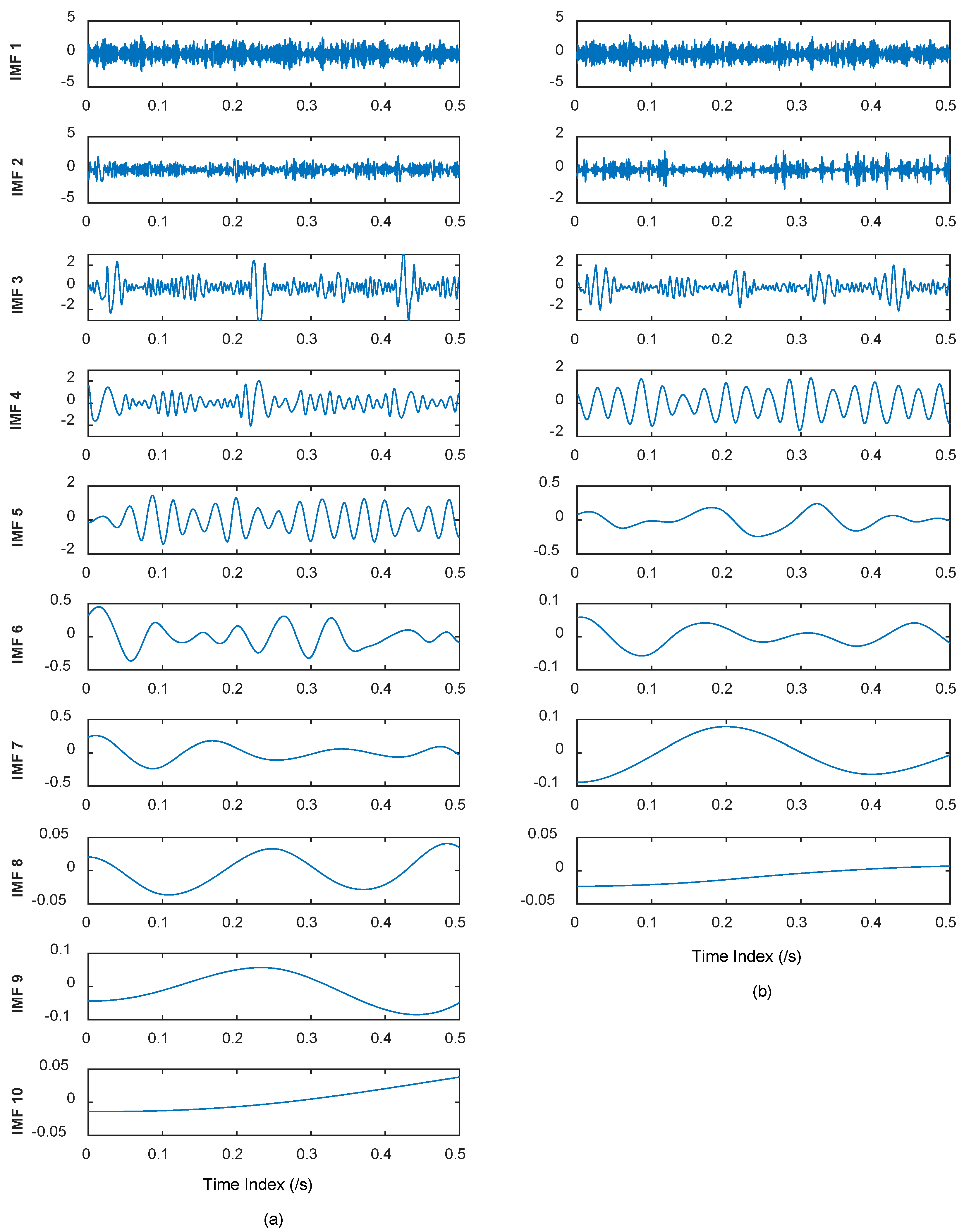
2.1. Complete Ensemble Empirical Mode Decomposition with Adaptive Noise
- (1)
- Given a signal x, and calculate all the maximum and minimum values of rk (k = 0), here rk = x.
- (2)
- Use the cubic spline to interpolate all maximum and minimum points of rk to obtain the upper and lower envelopes emax and emin, respectively.
- (3)
- Calculate the average of the upper and lower envelopes m = (emax + emin)/2.
- (4)
- Calculate the IMF by rk − m = hk+1, and decide if hk+1 satisfies the conditions of IMF, if not, repeat (2)–(3) to obtain the envelope average that satisfies the conditions.
- (5)
- Separate hk+1 from x to get rk+1, then let k = k + 1, repeat steps (2)–(4) with regarding rk as the original time series.
- (6)
- Repeat the above steps until the residual that meets the stop condition is obtained.
- (1)
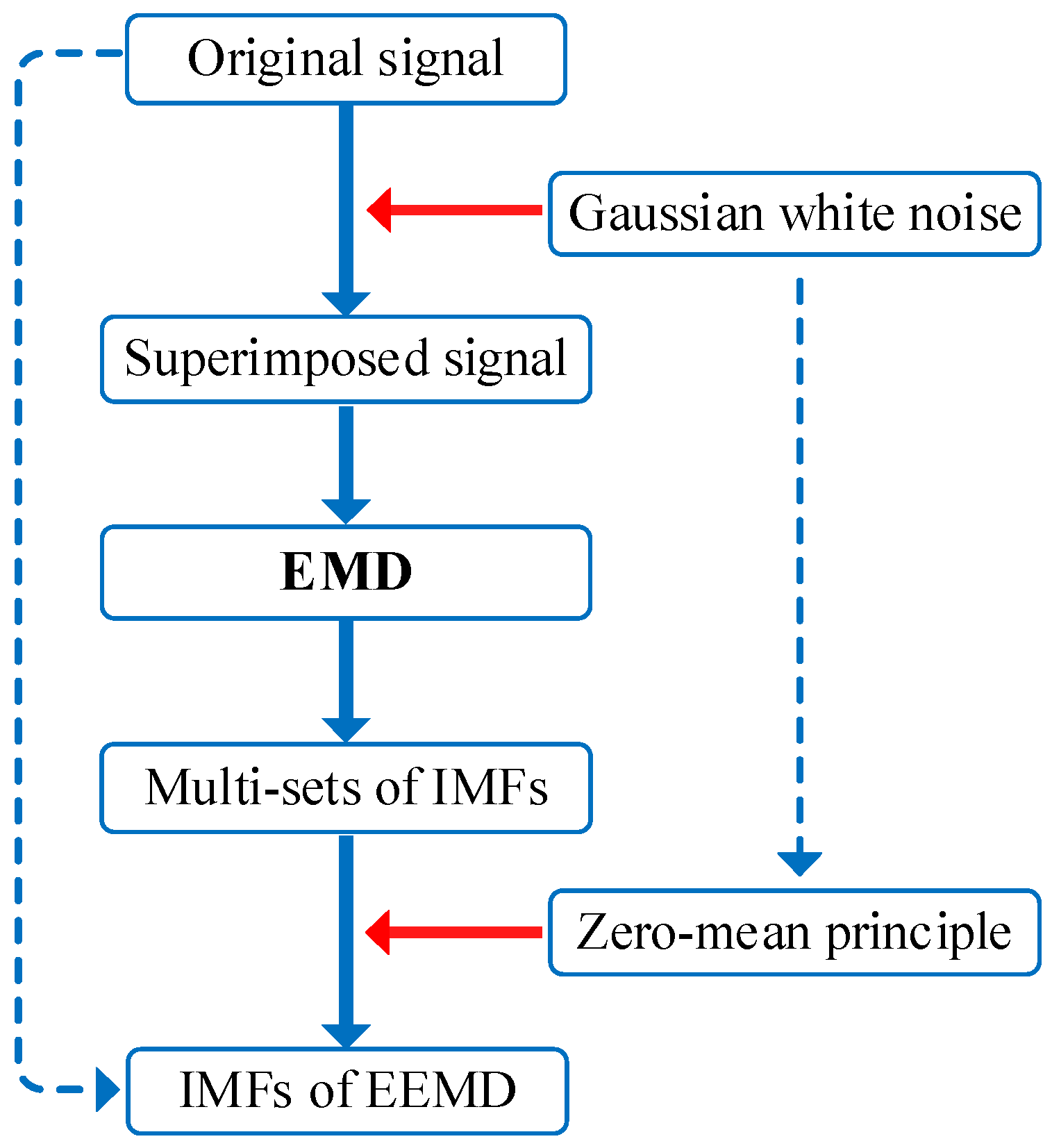
- Add Gaussian white noise to the signal to form a superimposed signal x(i) = x + εw(i).
- (2)
- Add Gaussian white noise to the signal to form a superimposed signal x(i) = x + εw(i).
- (3)
- Perform EMD of x(i) to obtain IMFs dk(i) (k = 1, …, K), K is the number of all IMFs:
- (4)
- Adopt the zero-mean principle of Gaussian white noise to eliminate the influence by taking Gaussian white noise as a time domain distribution reference structure. Then the IMFs can be expressed as:
- (1)
- Perform EMD towards x(i) = x + β0w(i) (i = 1, …, I), and the first order IMF is:
- (2)
- Compute the first residual:
- (3)
- Perform EMD to obtain the first IMF of r1 + β1E1(w(i)) (i = 1, …, I), and the second IMF is:
- (4)
- Compute kth residual for k = 2, 3, …, K:
- (5)
- Perform EMD to obtain the first IMF of rk + βkEk(w(i)) (i = 1, …, I), and the (k + 1)th IMF is:
- (6)
- Return to step (4) to compute the next order IMF, and repeat steps (4)–(6) until the residual cannot be decomposed by EMD. The coefficient βk = εk std(rk) allows the SNR to be selected during each iteration, and std(·) is the standard deviation operator.
2.2. Improved Multivariate Multiscale Sample Entropy
- (1)
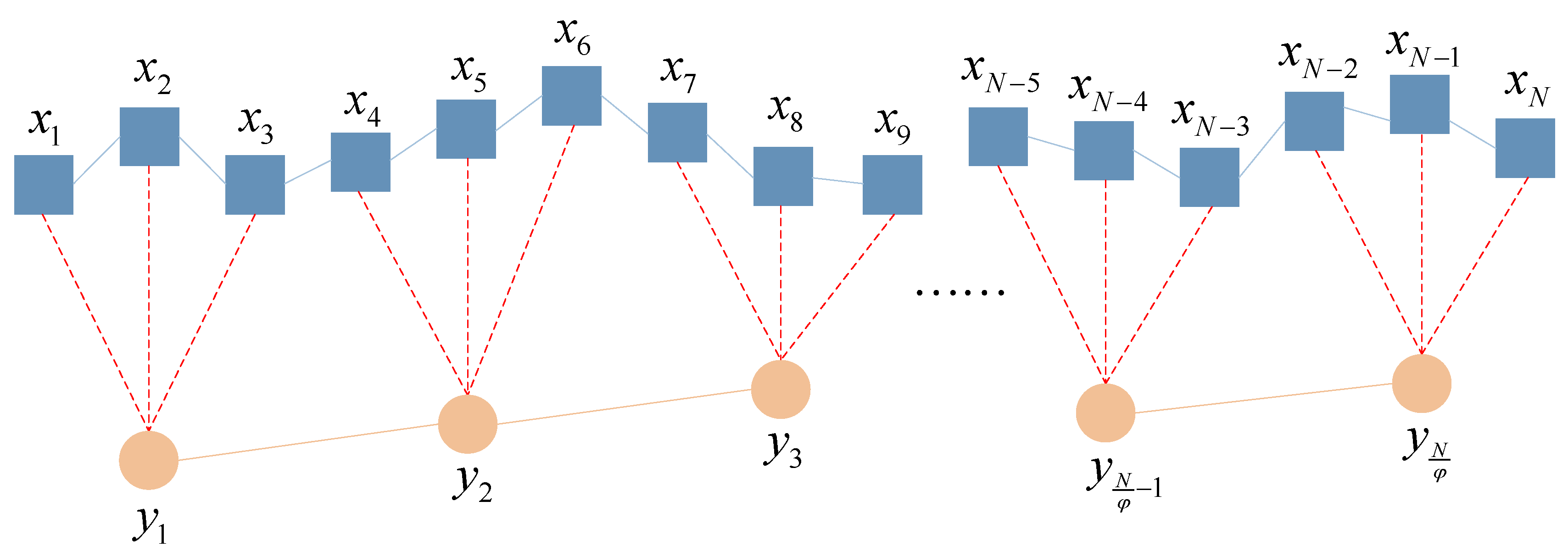
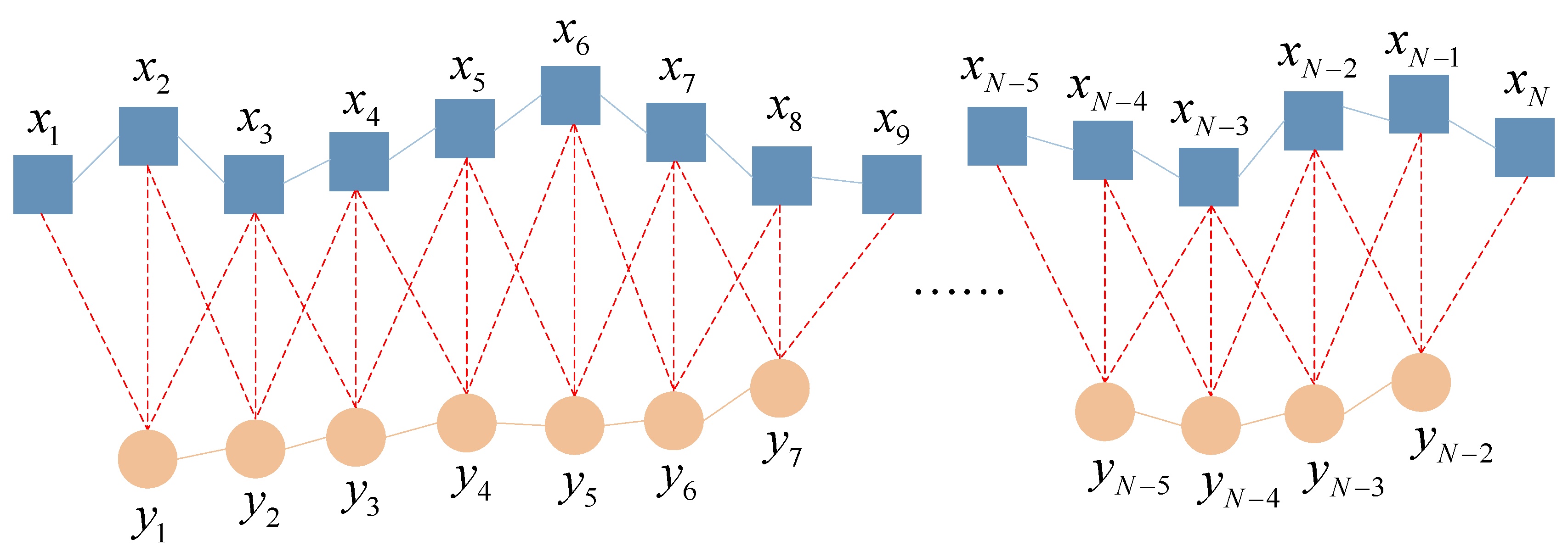
- For the original time series X = {x1, x2, …, xN}, X(i) = [xi, xi+1, …, xi+m−1], (1 ≤ i ≤ N − m) can be defined, m is the embedding dimension.
- (2)
- Compute dij (1≤ j ≤ N − m, j ≠ i) of X(i) and X(j), and calculate num(dij < r) when dij < r. dij is the maximum absolute value of difference of X(i) and X(j). Define Bim(r) = num(dij < r)/(N − m − 1).
- (3)
- Compute the mean value of Bim(r), denoted by Bm(r).
- (4)
- As for the dimension of m + 1, repeat above procedures to obtain Bim+1(r), then Bm+1(r) can be obtained.
- (5)
- The SE can be expressed as:
- (1)
- Constitute multivariate embedding vector Xm(i), and define the distance of any two vectors Xm(i) and Xm(j) as the maximum norm as follows:
- (2)
- As for the composite delay vector Xm(i) and a threshold r, determine the number of instances Pi, where D[Xm(i), Xm(j)] ≤ r, j ≠ i. Then compute the occurrence frequency Bim(r) = Pi/(N − n − 1), where n = max{M} × max{λ}.
- (3)
- Compute the average of B, denoted by Bm(r).
- (4)
- Extend the dimension of multivariate delay factor in (2) from m to (m + 1). Then, as for one embedding vector M = [m1, m2, …, mk…, mp], it can be converted into random space with the embedding vector of M = [m1, m2, …, mk+1…, mp] in p different ways. Thus, p × (N − n) vectors Xm+1(i) can be obtained in Rm+1, where Xm+1(i) represents any embedding vector which increases embedding dimension mk to (mk + 1) for specific k. Due to the constant of the embedding dimension of other data channels in this process, the overall embedding dimension of multivariate time series increases from m to (m +1).
- (5)
- Repeat procedures of (1)–(4) to compute all , and calculate the mean value Bim+1(r) upon k. Then compute the mean value Bm+1(r) upon i in the (m + 1) dimensional space as:Here, Bm (r) represents the similar possibility in m dimensional space of any two composite delay vectors, whereas Bm+1 (r) represents the similar possibility upon (m + 1) dimensional space of two composite delay vectors.
- (6)
- Then the MMSE can be expressed as:
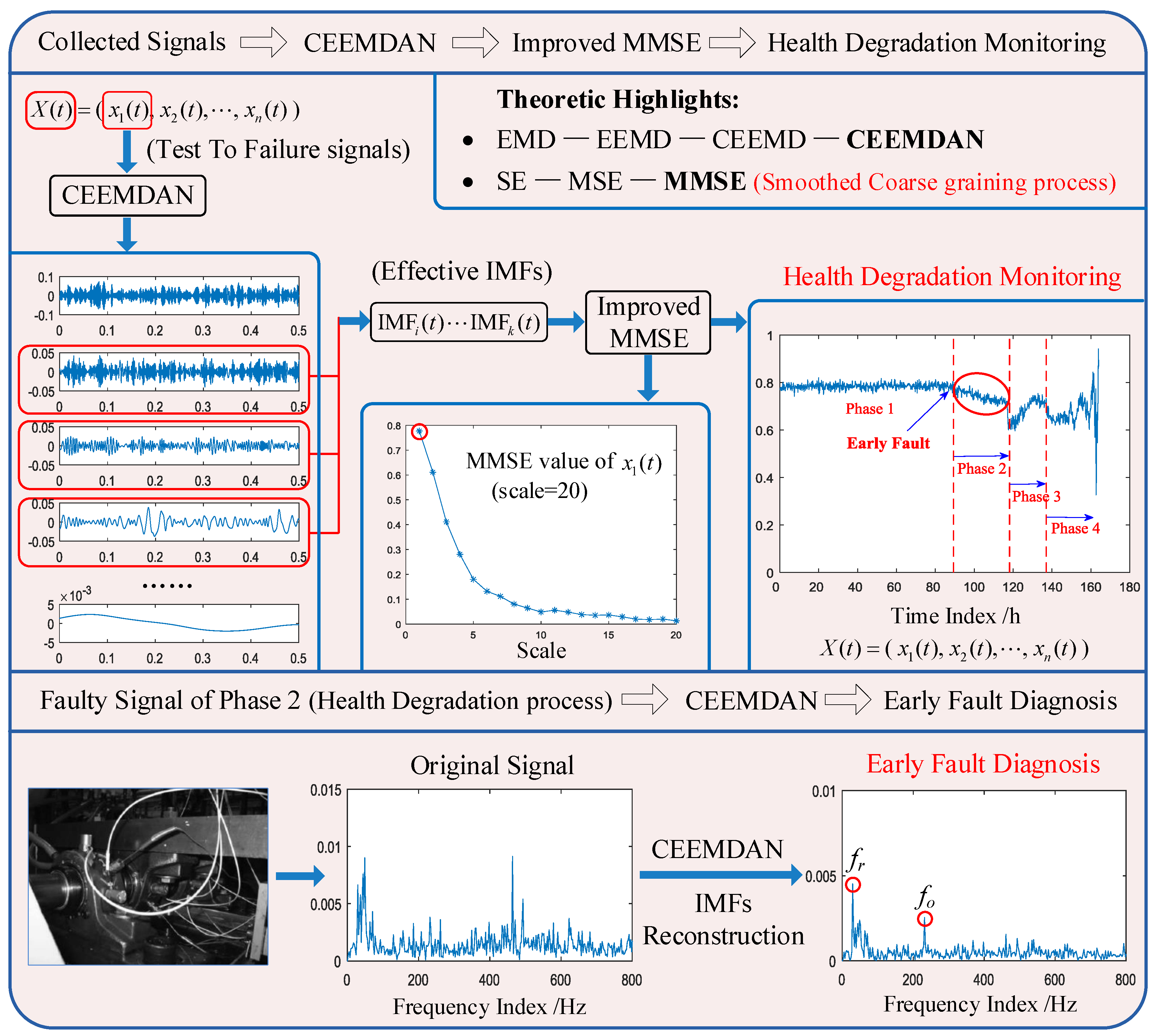
2.3. The Proposed Novel Health Degradation Monitoring Approach of Rolling Bearings
3. Numerical Simulations
3.1. Simulation Research of Complete Ensemble Empirical Mode Decomposition with Adaptive Noise
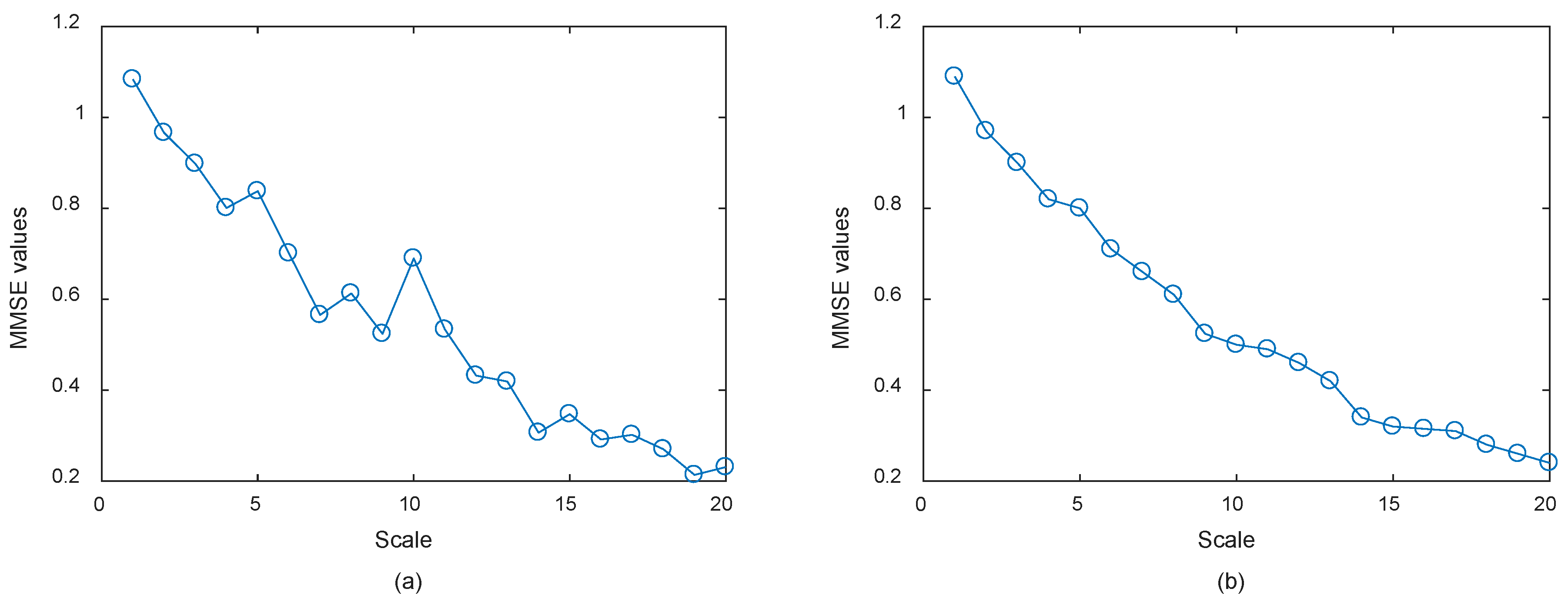
3.2. Simulation Research of Improved Multivariate Multiscale Sample Entropy
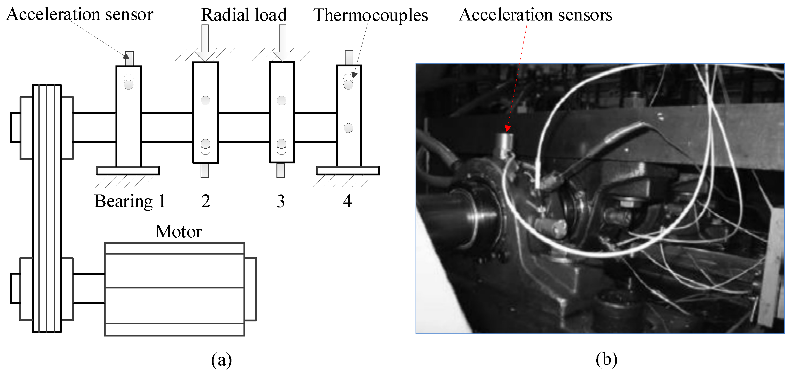
4. Application Studies on Health Degradation Monitoring and Early Fault Diagnosis of Rolling Bearings
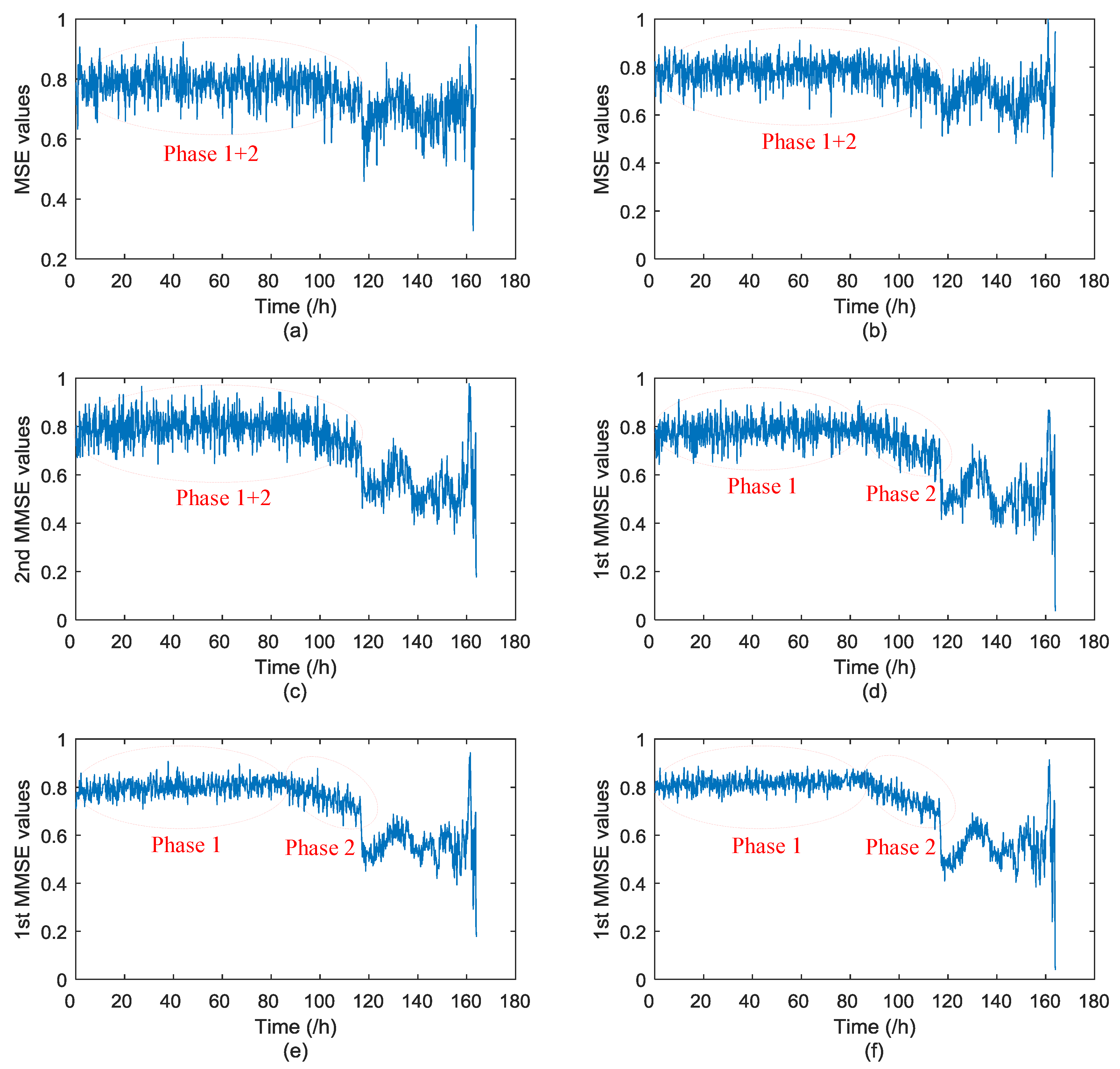
4.1. Application Studies of the Proposed Health Degradation Monitoring Method of Rolling Bearings
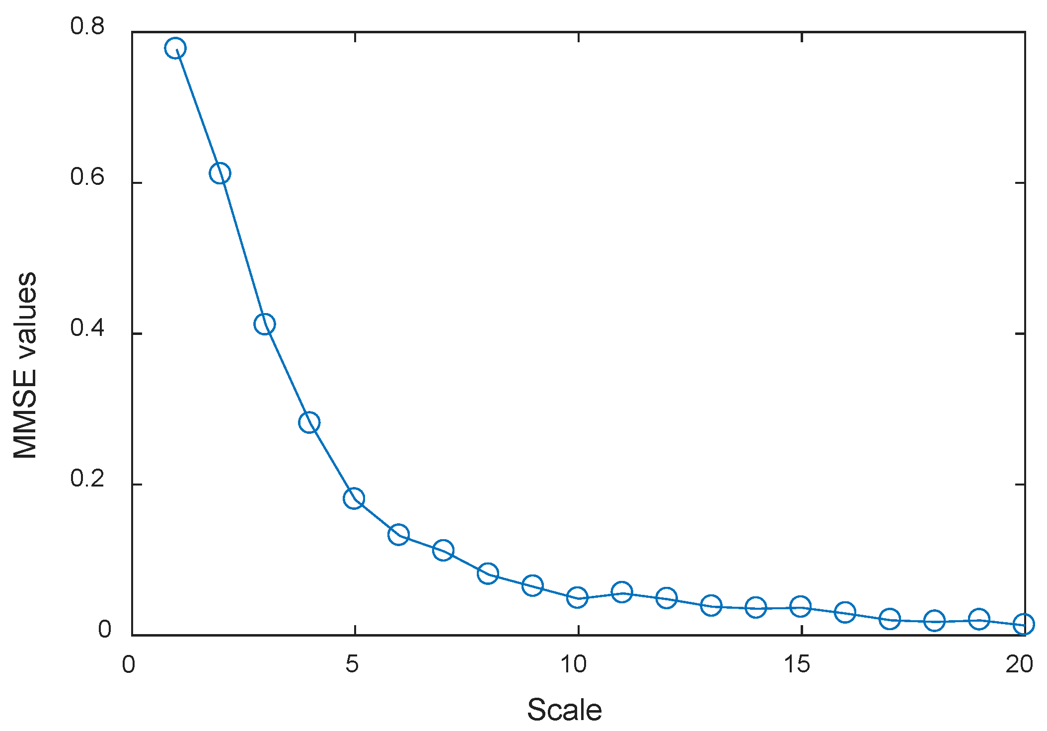
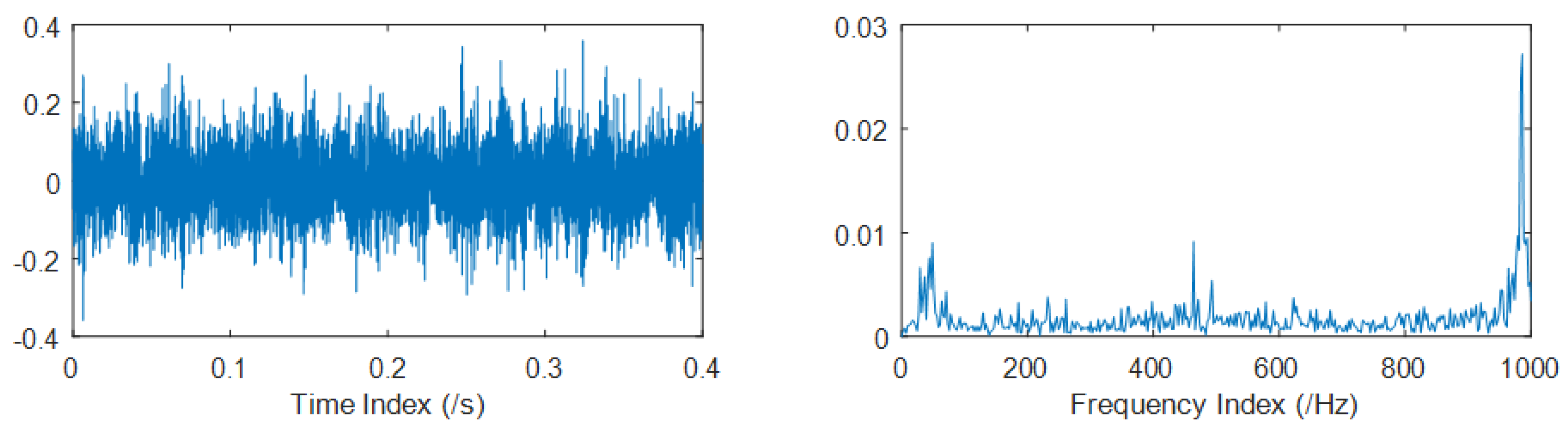
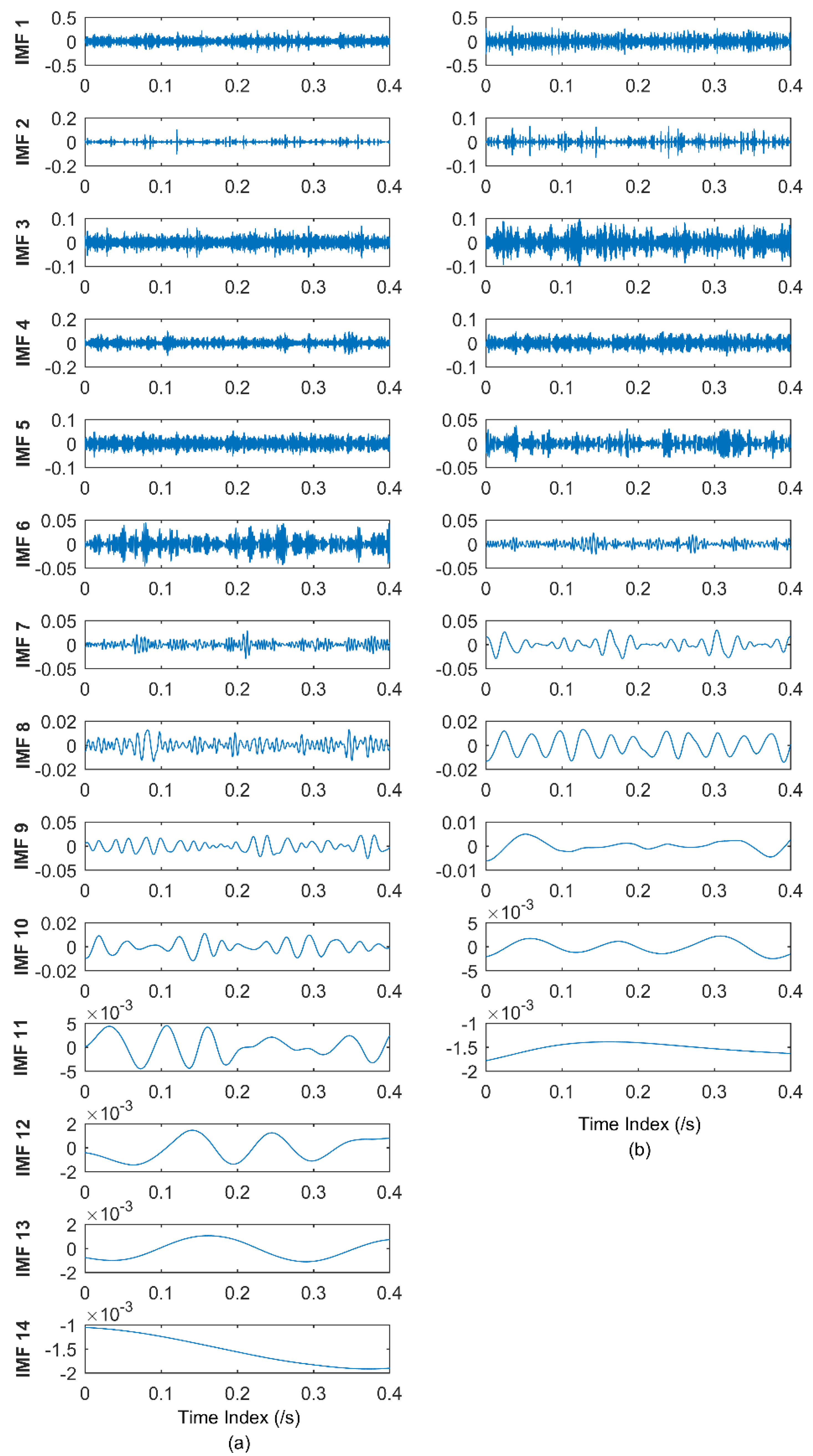
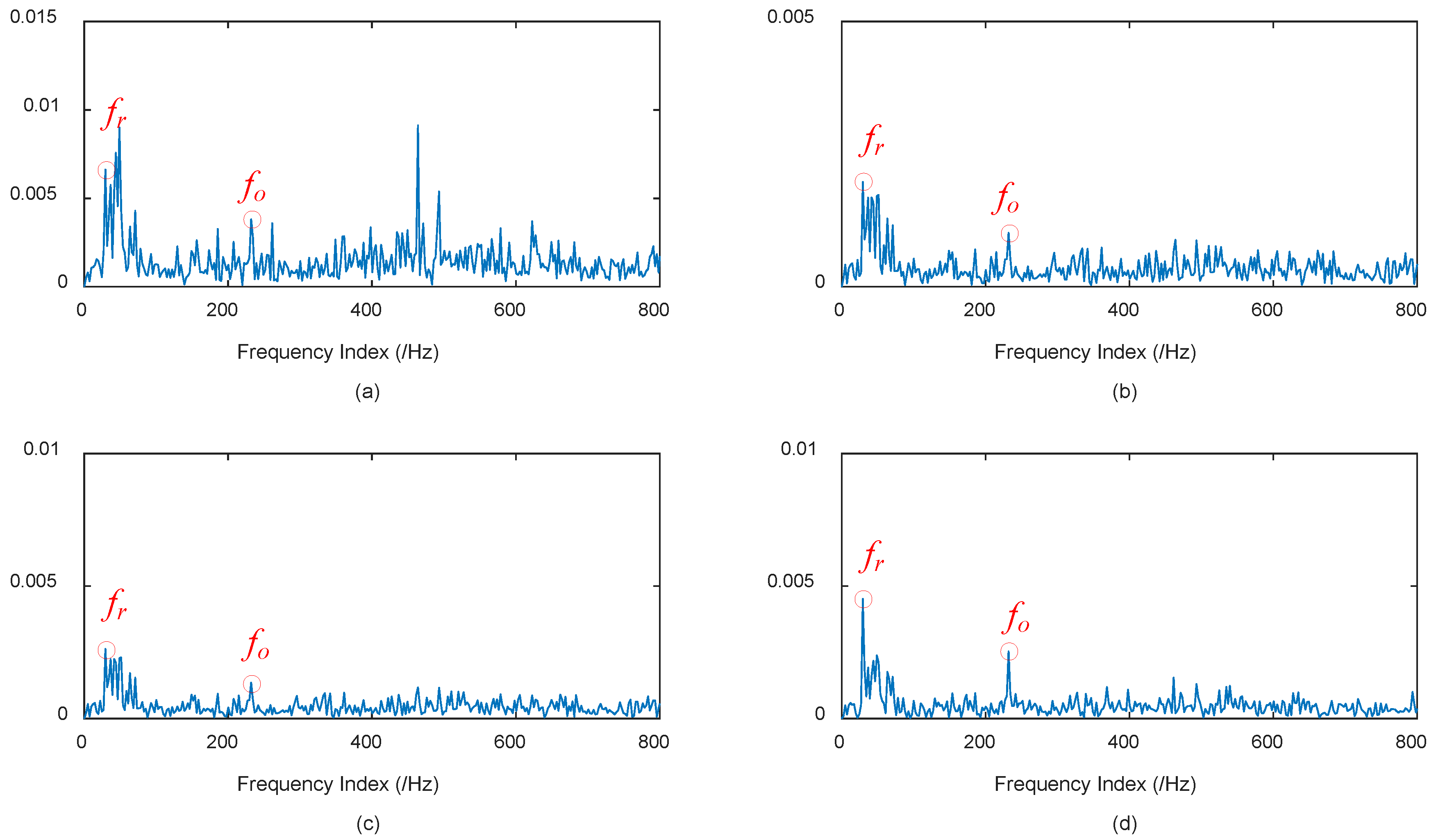
4.2. Application Research of the Proposed Early Fault Diagnosis Method of Rolling Bearings
5. Conclusions
Author Contributions
Funding
Acknowledgments
Conflicts of Interest
References
- Lei, Y.; Lin, J.; He, Z.; Zuo, M.J. A review on empirical mode decomposition in fault diagnosis of rotating machinery. Mechan. Syst. Signal Process. 2013, 35, 108–126. [Google Scholar] [CrossRef]
- Cerrada, M.; Sánchez, R.V.; Li, C.; Pacheco, F.; Cabrera, D.; de Oliveira, J.V.; Vásquez, R.E. A review on data-driven fault severity assessment in rolling bearings. Mechan. Syst. Signal Process. 2018, 99, 169–196. [Google Scholar] [CrossRef]
- Li, B.; Chow, M.Y.; Tipsuwan, Y.; Hung, J.C. Neural-network-based motor rolling bearing fault diagnosis. IEEE Trans. Ind. Electron. 2000, 47, 1060–1069. [Google Scholar] [CrossRef]
- Zhao, M.; Lin, J.; Xu, X.; Lei, Y. Tacholess envelope order analysis and its application to fault detection of rolling element bearings with varying speeds. Sensors 2013, 13, 10856–10875. [Google Scholar] [CrossRef] [PubMed]
- Yuan, J.; Wang, Y.; Peng, Y.; Wei, C. Weak fault detection and health degradation monitoring using customized standard multiwavelets. Mechan. Syst. Signal Process. 2017, 94, 384–399. [Google Scholar] [CrossRef]
- Yan, R.; Liu, Y.; Gao, R.X. Permutation entropy: A nonlinear statistical measure for status characterization of rotary machines. Mechan. Syst. Signal Process. 2012, 29, 474–484. [Google Scholar] [CrossRef]
- Shen, Z.; He, Z.; Chen, X.; Sun, C.; Liu, Z. A monotonic degradation assessment index of rolling bearings using fuzzy support vector data description and running time. Sensors 2012, 12, 10109–10135. [Google Scholar] [CrossRef] [PubMed]
- Xiao, H.; Zheng, J.; Song, G. Severity evaluation of the transverse crack in a cylindrical part using a PZT wafer based on an interval energy approach. Smart Mater. Struct. 2016, 25, 035021. [Google Scholar] [CrossRef]
- Lu, S.; Zhou, P.; Wang, X.; Liu, Y.; Liu, F.; Zhao, J. Condition monitoring and fault diagnosis of motor bearings using undersampled vibration signals from a wireless sensor network. J. Sound Vib. 2018, 414, 81–96. [Google Scholar] [CrossRef]
- Yu, J. Adaptive hidden Markov model-based online learning framework for bearing faulty detection and performance degradation monitoring. Mechan. Syst. Signal Process. 2017, 83, 149–162. [Google Scholar] [CrossRef]
- Xue, L.; Li, N.; Lei, Y.; Li, N. Incipient Fault Detection for Rolling Element Bearings under Varying Speed Conditions. Materials 2017, 10, 675. [Google Scholar] [CrossRef] [PubMed]
- Zhang, S.; Zhang, Y.; Li, L.; Wang, S.; Xiao, Y. An effective health indicator for rolling elements bearing based on data space occupancy. Struct. Health Monit. 2018, 17, 3–14. [Google Scholar] [CrossRef]
- Zhao, L.Y.; Wang, L.; Yan, R.Q. Rolling bearing fault diagnosis based on wavelet packet decomposition and multi-scale permutation entropy. Entropy 2015, 17, 6447–6461. [Google Scholar] [CrossRef]
- Zhong, J.; Huang, Y. Time-frequency representation based on an adaptive short-time Fourier transform. IEEE Trans. Signal Process. 2010, 58, 5118–5128. [Google Scholar] [CrossRef]
- Guo, Y.; Na, J.; Li, B.; Fung, R.F. Envelope extraction based dimension reduction for independent component analysis in fault diagnosis of rolling element bearing. J. Sound Vib. 2014, 333, 2983–2994. [Google Scholar] [CrossRef]
- Flandrin, P.; Rilling, G.; Goncalves, P. Empirical mode decomposition as a filter bank. IEEE Signal Process. Lett. 2004, 11, 112–114. [Google Scholar] [CrossRef]
- Gao, Z.; Lin, J.; Wang, X.; Xu, X. Bearing Fault Detection Based on Empirical Wavelet Transform and Correlated Kurtosis by Acoustic Emission. Materials 2017, 10, 571. [Google Scholar] [CrossRef] [PubMed]
- Huang, N.E.; Shen, Z.; Long, S.R.; Wu, M.C.; Shih, H.H.; Zheng, Q.; Yen, N.C.; Tung, C.C.; Liu, H.H. The empirical mode decomposition and the Hilbert spectrum for nonlinear and non-stationary time series analysis. Proc. Math. Phys. Eng. Sci. 1998, 454, 903–995. [Google Scholar] [CrossRef]
- Wu, Z.; Huang, N.E. Ensemble empirical mode decomposition: A noise-assisted data analysis method. Adv. Adapt. Data Anal. 2009, 1. [Google Scholar] [CrossRef]
- Sweeney, K.T.; McLoone, S.F.; Ward, T.E. The use of ensemble empirical mode decomposition with canonical correlation analysis as a novel artifact removal technique. IEEE Trans. Biomed. Eng. 2013, 60, 97–105. [Google Scholar] [CrossRef] [PubMed]
- Han, L.; Li, C.; Liu, H. Feature extraction method of rolling bearing fault signal based on EEMD and cloud model characteristic entropy. Entropy 2015, 17, 6683–6697. [Google Scholar] [CrossRef]
- Yeh, J.R.; Shieh, J.S.; Huang, N.E. Complementary ensemble empirical mode decomposition: A novel noise enhanced data analysis method. Adv. Adapt. Data Anal. 2010, 2, 135–156. [Google Scholar] [CrossRef]
- Torres, M.E.; Colominas, M.A.; Schlotthauer, G.; Flandrin, P. A complete ensemble empirical mode decomposition with adaptive noise. In Proceedings of the Acoustics, Speech and Signal Processing (ICASSP), 2011 IEEE International Conference, Prague, Czech Republic, 22–27 May 2011; pp. 4144–4147. [Google Scholar]
- Xu, Y.; Luo, M.; Li, T.; Song, G. ECG Signal De-noising and Baseline Wander Correction Based on CEEMDAN and Wavelet Threshold. Sensors 2017, 17, 2754. [Google Scholar] [CrossRef] [PubMed]
- Pincus, S.M. Approximate entropy as a measure of system complexity. Proc. Natl. Acad. Sci. USA 1991, 88, 2297–2301. [Google Scholar] [CrossRef] [PubMed]
- Alcaraz, R.; Rieta, J.J. A review on sample entropy applications for the non-invasive analysis of atrial fibrillation electrocardiograms. Biomed. Signal Process. Control 2010, 5, 1–14. [Google Scholar] [CrossRef]
- Bandt, C.; Pompe, B. Permutation entropy: A natural complexity measure for time series. Phys. Rev. Lett. 2002, 88, 174102. [Google Scholar] [CrossRef] [PubMed]
- Shi, Z.; Song, W.; Taheri, S. Improved LMD, Permutation Entropy and Optimized K-Means to Fault Diagnosis for Roller Bearings. Entropy 2016, 18, 70. [Google Scholar] [CrossRef]
- Ai, Y.T.; Guan, J.Y.; Fei, C.W.; Tian, J.; Zhang, F.L. Fusion information entropy method of rolling bearing fault diagnosis based on n-dimensional characteristic parameter distance. Mechan. Syst. Signal Process. 2017, 88, 123–136. [Google Scholar] [CrossRef]
- Chen, B.; Yan, Z.; Chen, W. Defect Detection for Wheel-Bearings with Time-Spectral Kurtosis and Entropy. Entropy 2014, 16, 607–626. [Google Scholar] [CrossRef]
- Chen, X.; Liu, D.; Xu, G.; Jiang, K.; Liang, L. Application of wavelet packet entropy flow manifold learning in bearing factory inspection using the ultrasonic technique. Sensors 2014, 15, 341–351. [Google Scholar] [CrossRef] [PubMed]
- Caesarendra, W.; Kosasih, B.; Tieu, A.K.; Moodie, C.A. Application of the largest Lyapunov exponent algorithm for feature extraction in low speed slew bearing condition monitoring. Mechan. Syst. Signal Process. 2015, 50, 116–138. [Google Scholar] [CrossRef]
- Wang, B.; Hu, X.; Li, H. Rolling bearing performance degradation condition recognition based on mathematical morphological fractal dimension and fuzzy C-means. Measurement 2017, 109, 1–8. [Google Scholar] [CrossRef]
- Humeau-Heurtier, A. The Multiscale Entropy Algorithm and Its Variants: A Review. Entropy 2015, 17, 3110–3123. [Google Scholar] [CrossRef]
- Wu, Y.; Shang, P.; Li, Y. Modified generalized multiscale sample entropy and surrogate data analysis for financial time series. Nonlinear Dyn. 2018, 92, 1335–1350. [Google Scholar] [CrossRef]
- Wu, S.D.; Wu, C.W.; Lin, S.G.; Wang, C.C.; Lee, K.Y. Time series analysis using composite multiscale entropy. Entropy 2013, 15, 1069–1084. [Google Scholar] [CrossRef]
- Ahmed, M.U.; Mandic, D.P. Multivariate Multiscale Entropy Analysis. IEEE Signal Proces. Lett. 2012, 19, 91–94. [Google Scholar] [CrossRef]
- Yin, Y.; Shang, P. Multivariate multiscale sample entropy of traffic time series. Nonlinear Dyn. 2016, 86, 479–488. [Google Scholar] [CrossRef]
- Wei, Q.; Liu, D.H.; Wang, K.H.; Liu, Q.; Abbod, M.F.; Jiang, B.C.; Chen, K.P.; Wu, C.; Shieh, J.S. Multivariate Multiscale Entropy Applied to Center of Pressure Signals Analysis: An Effect of Vibration Stimulation of Shoes. Entropy 2012, 14, 2157–2172. [Google Scholar] [CrossRef]
- Wang, G.F.; Li, Y.B.; Luo, Z.G. Fault classification of rolling bearing based on reconstructed phase space and Gaussian mixture model. J. Sound Vib. 2009, 323, 1077–1089. [Google Scholar] [CrossRef]
- Barnard, J.P.; Aldrich, C.; Gerber, M. Embedding of multidimensional time-dependent observations. Phys. Rev. E 2001, 64, 046201. [Google Scholar] [CrossRef] [PubMed]
- Looney, D.; Hemakom, A.; Mandic, D.P. Intrinsic multi-scale analysis: A multi-variate empirical mode decomposition framework. Proc. R. Soc. A 2015, 471, 20140709. [Google Scholar] [CrossRef] [PubMed]
- Sharma, R.; Pachori, R.; Acharya, U. Application of Entropy Measures on Intrinsic Mode Functions for the Automated Identification of Focal Electroencephalogram Signals. Entropy 2015, 17, 669–691. [Google Scholar] [CrossRef]
- Sharma, R.; Pachori, R.B. Classification of epileptic seizures in EEG signals based on phase space representation of intrinsic mode functions. Expert Syst. Appl. 2015, 42, 1106–1117. [Google Scholar] [CrossRef]
- Hu, M.; Liang, H. Intrinsic mode entropy based on multivariate empirical mode decomposition and its application to neural data analysis. Cognit. Neurodyn 2011, 5, 277–284. [Google Scholar] [CrossRef] [PubMed]
- Rai, V.K.; Mohanty, A.R. Bearing fault diagnosis using FFT of intrinsic mode functions in Hilbert–Huang transform. Mechan. Syst. Signal Process. 2007, 21, 2607–2615. [Google Scholar] [CrossRef]
- Wu, W.; Chen, X.; Su, X. Blind Source Separation of Single-channel Mechanical Signal Based on Empirical Mode Decomposition. J. Mechan. Eng. 2011, 47, 12. [Google Scholar] [CrossRef]
- Lee, S.K.; White, P.R. The enhancement of impulsive noise and vibration signals for fault detection in rotating and reciprocating machinery. J. Sound Vib. 1998, 217, 485–505. [Google Scholar] [CrossRef]
- Lv, Y.; Yuan, R.; Song, G. Multivariate empirical mode decomposition and its application to fault diagnosis of rolling bearing. Mechan. Syst. Signal Process. 2016, 81, 219–234. [Google Scholar] [CrossRef]
- Yuan, R.; Lv, Y.; Song, G. Multi-Fault Diagnosis of Rolling Bearings via Adaptive Projection Intrinsically Transformed Multivariate Empirical Mode Decomposition and High Order Singular Value Decomposition. Sensors 2018, 18, 1210. [Google Scholar] [CrossRef] [PubMed]
- Qiu, H.; Lee, J.; Lin, J.; Yu, G. Wavelet filter-based weak signature detection method and its application on rolling element bearing prognostics. J. Sound Vib. 2006, 289, 1066–1090. [Google Scholar] [CrossRef]


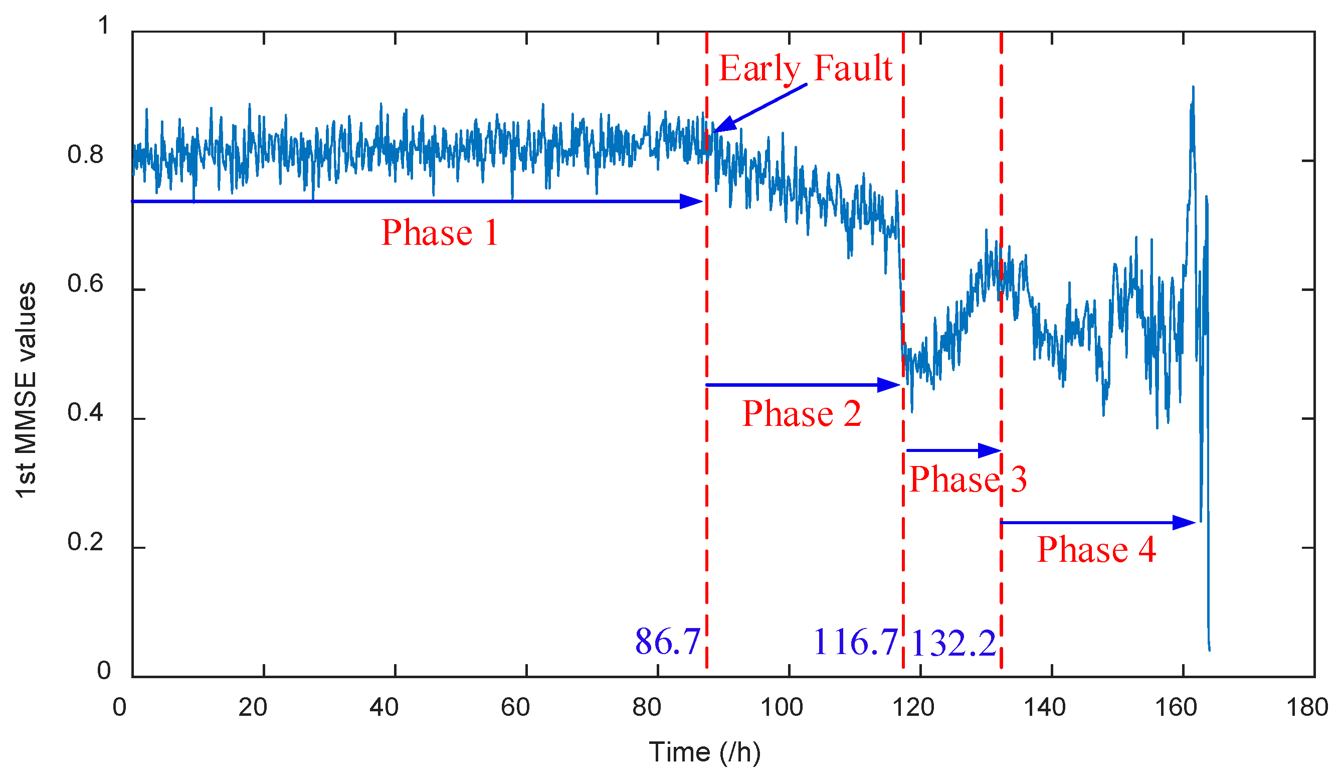
| Phase 1 | The bearing is operating normally, prior to the occurrence of the early weak fault. |
| Phase 2 | The early weak fault occurs on the rolling bearing and interferes with its running condition slightly; this is the initial phase of early weak fault. |
| Phase 3 | The fault develops into the middle stage, generating the self-balancing and self-healing phenomenon, also called the retardation effect. This is the phase that the rolling bearing fault tends to be serious. |
| Phase 4 | The rolling bearing deteriorates promptly and has a serious fault. It usually results in the final breakdown of the rolling bearing. |
| Methods | Phase 1 | Phase 2 | |
|---|---|---|---|
| Variance | Variance | Slope | |
| MMSE (Conventional coarse graining) | 0.78 × 10⁻³ | 2.21 × 10⁻³ | −6.80 × 10⁻⁴ |
| MMSE (Smoothed coarse graining) | 0.34 × 10⁻³ | 1.16 × 10⁻³ | −7.92 × 10⁻⁴ |
| Detailed Parameters of Rexnord ZA-2115 Rolling Bearing | |||
|---|---|---|---|
| Ball number n | Contact angle α | Ball diameter dr | Pitch diameter Dw |
| 16 | 15.17 | 0.331 | 2.815 |
| Fault Type | Fault Frequency Computation | Fault Frequency |
|---|---|---|
| Outer ring fault | fo = 0.5n(1 − drcosα/Dw)fr | fo = 236.4 |
© 2018 by the authors. Licensee MDPI, Basel, Switzerland. This article is an open access article distributed under the terms and conditions of the Creative Commons Attribution (CC BY) license (http://creativecommons.org/licenses/by/4.0/).
Share and Cite
Lv, Y.; Yuan, R.; Wang, T.; Li, H.; Song, G. Health Degradation Monitoring and Early Fault Diagnosis of a Rolling Bearing Based on CEEMDAN and Improved MMSE. Materials 2018, 11, 1009. https://doi.org/10.3390/ma11061009
Lv Y, Yuan R, Wang T, Li H, Song G. Health Degradation Monitoring and Early Fault Diagnosis of a Rolling Bearing Based on CEEMDAN and Improved MMSE. Materials. 2018; 11(6):1009. https://doi.org/10.3390/ma11061009
Chicago/Turabian StyleLv, Yong, Rui Yuan, Tao Wang, Hewenxuan Li, and Gangbing Song. 2018. "Health Degradation Monitoring and Early Fault Diagnosis of a Rolling Bearing Based on CEEMDAN and Improved MMSE" Materials 11, no. 6: 1009. https://doi.org/10.3390/ma11061009
APA StyleLv, Y., Yuan, R., Wang, T., Li, H., & Song, G. (2018). Health Degradation Monitoring and Early Fault Diagnosis of a Rolling Bearing Based on CEEMDAN and Improved MMSE. Materials, 11(6), 1009. https://doi.org/10.3390/ma11061009