A Statistical Framework for Automatic Leakage Detection in Smart Water and Gas Grids

Abstract

In the last few years, due to the technological improvement of advanced metering infrastructures, water and natural gas grids can be regarded as smart-grids, similarly to power ones. However, considering the number of studies related to the application of computational intelligence to distribution grids, the gap between power grids and water/gas grids is notably wide. For this purpose, in this paper, a framework for leakage identification is presented. The framework is composed of three sections aimed at the extraction and the selection of features and at the detection of leakages. A variation of the Sequential Feature Selection (SFS) algorithm is used to select the best performing features within a set, including, also, innovative temporal ones. The leakage identification is based on novelty detection and exploits the characterization of a normality model. Three statistical approaches, The Gaussian Mixture Model (GMM), Hidden Markov Model (HMM) and One-Class Support Vector Machine (OC-SVM), are adopted, under a comparative perspective. Both residential and office building environments are investigated by means of two datasets. One is the Almanac of Minutely Power dataset (AMPds), and it provides water and gas data consumption at 1, 10 and 30 min of time resolution; the other is the Department of International Development (DFID) dataset, and it provides water and gas data consumption at 30 min of time resolution. The achieved performance, computed by means of the Area Under the Curve (AUC), reaches $90\%$ in the office building case study, thus confirming the suitability of the proposed approach for applications in smart water and gas grids.

1. Introduction

Differently from city-wide distribution grids, residential and building networks can be affected by very small leakages, which can be detected only after lengthy or complex actions, e.g., comparing winter usage or checking measured resource intake at the meter during periods of no resource usage. They may remain unnoticed for weeks or months, thus producing huge waste or even damage. As a matter of fact, the statistics reported in the WaterSense Project [1] show that residential water leaks, in the U.S., waste about $3.78$ trillion liters annually nationwide.

Many shortcomings still affect the development of proper applications for water and natural gas grids’ monitoring, as reported in the comprehensive survey by Fagiani et al. [2], despite the availability of advanced metering systems [3,4,5] andsensor fault diagnosis frameworks [6,7]. Specifically, in recent years, a wide set of machine learning and computational intelligence approaches have been focusing on the fulfillment of the smart-home and the smart-grid paradigms. Unfortunately, the energy field has drawn great attention [8], thus the water and natural gas fields have been left aside.

Water and natural gas are resources as precious as electrical energy. In a smart-home that follows the smart-grid paradigm, their monitoring should be added alongside the monitoring of electrical energy. Information and Communication Technologies (ICT) can provide the required real-time monitoring and control [9], thus integrating water, gas and electrical energy data into existing management systems [10,11], further improving their performance.

To investigate the problem, the authors’ focus has been aimed, in the first place, at consumption forecasting for short- and medium-term prediction in both residential and building scenarios [12], thus highlighting the effect of the grid scale on the consumption trends. Thereafter, since leakage detection in large-scale grids has been investigated in the literature, we focused on the detection of leakages occurring in water and natural grids of residential environments [13].

In this paper, the authors propose a framework to detect the presence of leakages in water and natural gas networks in both residential and building environments. The Gaussian Mixture Model (GMM), the Hidden Markov Model (HMM) and One-Class Support Vector Machine (OC-SVM) are adopted, under a comparative perspective, as statistical modeling approaches. Moreover, the framework extracts a set of features and performs a selection, by exploiting a proposed variation of the Sequential Feature Selection (SFS), to identify the best ones.

1.1. State of the Art

Novelty detection techniques raised deep interest in many application fields, and a large corpus of literature has been produced so far [14,15,16]. Among these, non-intrusive techniques [17,18] have been deemed of particular interest since they do not require additional tools, other than the water meter, to locate the leakage. Furthermore, many publications about leakage/fault detection in industrial environments are available in the literature. Aimed mostly at oil and natural gas pipelines, they are based on high sampling rates and/or multiple sensing points arranged along the pipeline. Since these methods are too invasive for residential environments, only the state of the art for civil resources’ distribution is presented below. Studies based on district network data have been included to evaluate the suitability of the proposed technique for office buildings, scenarios that have not been addressed, as of yet, in the current literature, as shown in

Table 1. Summary of the existing contributions in the leakage detection field and their characteristics. The “Target” columns report the target scenario, thus Residential (R) or District (D). The “Data” column reports the used data type, Flow (F) or Pressure (P), while the resource types, Water (W) or Gas (G), are reported in the column “Resource”. MNF, Minimum Night Flow.

Contribution	Target	Data	Resource	Technique	Main Issues
Alkasseh et al. [24]	D	F and P	W	MNF-MLR	Indirect detection 2 sensors No novelty approach
Gamboa-Medina et al. [22]	-	P	W	C4.5	Laboratory circuit 15 sensors No novelty approach
Mounce et al. [19]	D	F and P	W	SVR	Anomalies detection
Nasir et al. [20]	R	F and P	W	SVM and ANN	No real data 6 sensors No novelty approach
Oren and Stroh [25]	R	F	W	Heuristic	Ad hoc constraints No validation
Sanz et al. [23]	D	F	W	Fuzzy logic	2 sensors No novelty approach
Wan et al. [26]	-	F and P	G	SVM	5 acoustic and pressure sensors High-pressure pipe No novelty approach

.

Mounce et al. [19] have exploited the Support Vector Regression (SVR) technique in order to detect anomalies in time series of a water distribution system. The approach has proposed both flow and pressure analysis, and different types of novelty events have been tested, i.e., bursts, low pressure and large unusual demands. The evaluations have been performed by adopting the time series collected in 200 District Metered Areas (DMAs) by smart meters, with a sampling rate of 15 min. Experiments have been conducted to detect abnormal events and to analyze historical data. In the case of novelty detection experiments, the SVR model has been trained on a dataset spanning over 12 weeks, and the test has been performed over nine days worth of data, also containing the samples relating to abnormal events. On the other hand, for the historical evaluations, six months of data have been used in the testing phase, whereas the training has been performed on the prior six month subset.

Support Vector Machine (SVM) and Artificial Neural Network (ANN) have been recently exploited by Nasir et al. [20]. The experiments have been performed in order to estimate both the position and size of water leakages. The EPANET tool [21] has been adopted to simulate a residential network with two pressure sensors, two differential pressure sensors, two flow sensors and to acquire the data in the simulation circuit. About 1800 scenarios have been adopted to train the models, and an additional 1800 scenarios have been used to test them. The performance has been evaluated in terms of MSE and the squared correlation error coefficient (R-square). The proposed quasi-static analysis confirmed the good behavior of the SVM and its resilience to sensor measurement errors.

A binary classifier, referred to as C4.5, has been used by Gamboa-Medina et al. [22] to evaluate and to generate a set of rules to discriminate water leakages. In a controlled experimental laboratory circuit, water pressure data have been collected at high sampling rate (4 samples/s) by 15 sensors, producing 1-min sequences of 240 samples. Three-hundred ten no-leak and 310 leak sequences have been acquired and four features extracted: energy, entropy, zero crossing count and the distribution of the energy on the components of the wavelet decomposition. Single features and their combinations have been evaluated in terms of the Receiver Operating Characteristic (ROC) and Area Under the Curve (AUC). The 10-fold cross-validation method has been applied to train the classifier and to discriminate two classes, that is leak and no-leak.

Fuzzy logic has been applied to detect and locate leakages in water networks by Sanz et al. [23]. The proposed Fuzzy Inductive Reasoning (FIR) is composed of four main stages: fuzzification, qualitative modeling, qualitative simulation and defuzzification. The experiments have been performed by adopting 30 days of DMA pressure data, collected by two sensors at an hourly rate. The classification has been performed by training the system on the first three weeks of data; whereas tests have been performed on the remaining data synthetically modified by means of the EPANET [21] software: US EPA Research, Durham, NC, USA. The detection performance has been evaluated by pointing out the total amount of leakages detected in the various experiments. The proposed approach isolates correctly the leakages and presents a good precision.

Alkasseh et al. [24] have exploited a multiple linear regression (MLR) method to correlate the minimum night flow and a set of network parameters, such as the number of connections, the total length of pipe and the weighted mean age pipe of the network. The relation has been computed through the analysis of 30 DMAs’ data, and the difference between the actual MNF (Minimum Night Flow) and the estimated one, which could allow one to establish the presence of a leakage, has been evaluated by using R and R-square.

The mathematical model proposed by Oren and Stroh [25] is focused on the residential scenario. A set of heuristic thresholds, applied to flow data, have been defined to detect the presence of leakages. The approach exploits the data acquired in one sensing point, but neither exhaustive experiments nor evaluation criteria have been presented.

In the natural gas field, Wan et al. [26] have exploited a multi-classifier based on SVM in order to detect and localize leakages. The wavelet decomposition has been exploited to detect the leakage presence, whereas the difference of arrival have been adopted to estimate the leakage position. The manuscript reports that the experiments have been performed on an experimental circuit with five acoustic sensors that collect data at 1 MHz. One hundred twenty sequences, with and without leakages, have been adopted during the evaluations, and the training has been performed on $50\%$ of them and the test on the remaining sequences.

1.2. Literature Review

Most of the literature approaches have been tested on residential-sized or district-sized networks, as reported in Table 1. To our knowledge, most of them [19,20,22,23,24,26] cannot be applied to residential scenarios, where only aggregated flow measurement records are available, i.e., only one sensing point. Specifically, the input data in Nasir et al. [20] have been generated by means of the EPANET software [21] to simulate four pressure sensors and two flow sensors. The same tool, in Sanz et al. [23], has been used to simulate the presence of leakages in a DMA of Barcelona, called Nova Icària. In this case, non-faulty instances have been recorded by two pressure sensors, whereas the faulty instances have been simulated accordingly to that setup. Furthermore, in Gamboa-Medina et al. [22], the data have been collected by an experimental circuit of 15 pressure sensors arranged along the pipe. Finally, in Alkasseh et al. [24] and Mounce et al. [19], both flow and pressure data have been collected from DMAs. Mounce et al. [19] have correlated the anomalies in flow and pressure series with operational information and manual data interpretation. Wan et al. [26] have adopted a high-pressure experimental circuit with five acoustic and pressure sensors.

The only suitable approach, Oren and Stroh [25], which uses a single sensing point in a residential environment, shows some limitations, as well. First of all, the applied constraints have been computed from the average domestic water usage of several nations; therefore, the statistical information has not been obtained from the sequence itself. Moreover, the approach seems to lack proper experimental validation, by presenting one evaluation only.

The state of the art methods present many shortcomings, in addition to the number of data sources, even from the computational approach standpoint. In particular, the experimental methodology adopted in Alkasseh et al. [24], Gamboa-Medina et al. [22], Nasir et al. [20], Sanz et al. [23] and Wan et al. [26] is incompatible with the novelty detection paradigm [27,28], in which only the normal behavior is known. In Gamboa-Medina et al. [22], the binary classifier has been trained to discriminate two classes: leak and no-leak. In Nasir et al. [20], ANN and SVM have been trained to discriminate the leakage location and size; whereas Alkasseh et al. [24] do not discriminate the presence of a leakage, but a linear correlation between the MNF (Minimum Night Flow) loss and the number of connections, the total length of the pipe network and the pipes’ weighted mean age has been explicated.

On the other hand, in Mounce et al. [19] and Oren and Stroh [25], no faulty instances have been used to train the system, and the leakage scenario has been adopted only during the validation stage, in accordance with the novelty detection concept.

Among the reported contributions, several evaluation criteria have been adopted. Specifically, Oren and Stroh [25] and Mounce et al. [19] did not present a standard evaluation criterion.

1.3. Innovative Contribution

In this study, the authors propose a leakage detection framework based on statistical modeling that is focused on two distinct environments. They are named residential and building. The former deals with the consumption of a typical living environment, e.g., a house inhabited by one to six residents, whereas the latter refers to an office building with hundreds of occupants. In both scenarios, the consumption, that is flow data, is collected at a single sensing point with a sampling rate between 1 and 30 min. The Almanac of Minutely Power dataset (AMPds) [29] and the Department of International Development (DFID) dataset [30] have been used to represent these scenarios.

The method adopted in this framework has been inspired by the works of Principi et al. [31] and Kuncheva [32], where an audio novelty detection is performed by exploiting a statistical model of the normal condition of the system. The statistical approach in novelty detection has never been used for leakage identification, and within the state of the art, none of the contributions seem aimed at residential or building environments. Specifically, to the best of the authors’ knowledge, among recent studies, no one has targeted the natural gas grid in a residential scenario and water and gas grids in a building scenario.

In the proposed framework, each dataset has been split into overlapped frames, then a set of features, chosen by the authors, has been extracted. Indeed, in the literature, a well-defined set of features suitable for this application is yet to be proposed, and our contribution fills the gap. Moreover, a suitable feature selection stage has been proposed and adopted to determine the best combination of features for the diverse operative conditions.

In order to limit the number of tested combinations, a variation of the SFS [33] has been proposed. At the same time, to lower the chance of missing a good combination, rather than choosing only one feature, the three best features are selected at the end of the first step. The set of features, extracted during the training from the dataset, which is leakage free, has been used to characterize the normal behavior of the consumption, also called background model or normality background. The process has been carried out by means of GMM, HMM, and OC-SVM.

In the validation phase, the logarithmic likelihood values, or the distances to the hyperplane, of the new data have been computed by adopting the pre-trained background models, and a set of thresholds has been used to determine the True Detection Rate (TDR) and the False Detection Rate (FDR).

In the evaluation of the system performance, the validation sets have been manipulated by introducing artificial leakages in the records, and a leakage size between $25\%$ and $50\%$ of the average consumption of the training set has been assumed. The correctness of the modeled leakage records has been confirmed in a comparison against the ones collected in a real-life case environment [34].

In a residential scenario and based on the AMPds’ values, a leakage value spanning from $25\%$ to $50\%$ of the average consumption level, corresponds to values between 7.76 L/h and 15.53 L/h. In a real-life environment, the most common leakage rates are 20 L/h and 10 L/h, whereas $49\%$ of leakages are at most equal to 20 L/h, thus proving the correctness of the modeling criteria. To further improve the model, the leakage size, as well as the duration and the starting point, have been randomly selected. Specifically, a limited duration of the leakages has been chosen in order to simulate the correct detection of the anomaly and consequent restoration of standard operating conditions within the same observation window.

In order to provide an extensive study by exploiting the framework, the experiments proposed in Fagiani et al. [13] have been extended, as shown in the following. First, the experiments performed with residential consumption values, of water and natural gas, contained in AMPds, and at 1- and 10-min resolution, have been integrated by adding evaluations at 30 min of resolution. To this end, a new dataset has been introduced, namely the DFID dataset, which provides the records of the water and natural gas consumption of two buildings. Moreover, the feature set has been extended, as well. Along with the 10 features, originally proposed in Fagiani et al. [13], an extra set of temporal features has been included. The aim of these temporal features is to model any correlation between consumption levels and time, such as high consumption at peak hours or low consumption at night ones. In addition, a further statistical approach for the creation of the normality model has been evaluated, the One-Class Support Vector Machine (OC-SVM). As for GMM and HMM, the OC-SVM is a well-known approach for novelty detection, but it has never been adopted for the detection of water and gas losses in residential and building scenarios. In the experiments, the feature selection has been performed with and without the temporal features. Furthermore, an analysis of the performance variability has been carried out by keeping two leakage parameter fixed at a time and randomly varying the remaining one.

To conclude, the paper outline is presented. The proposed statistical framework for automatic leakage detection is introduced in Section 2. The Section also presents the adopted features, the statistical models used for novelty detection and the proposed SFS procedure. The experiments are presented and discussed in Section 3. The results are commented on and analyzed in Section 4, whereas Section 5 concludes the paper.

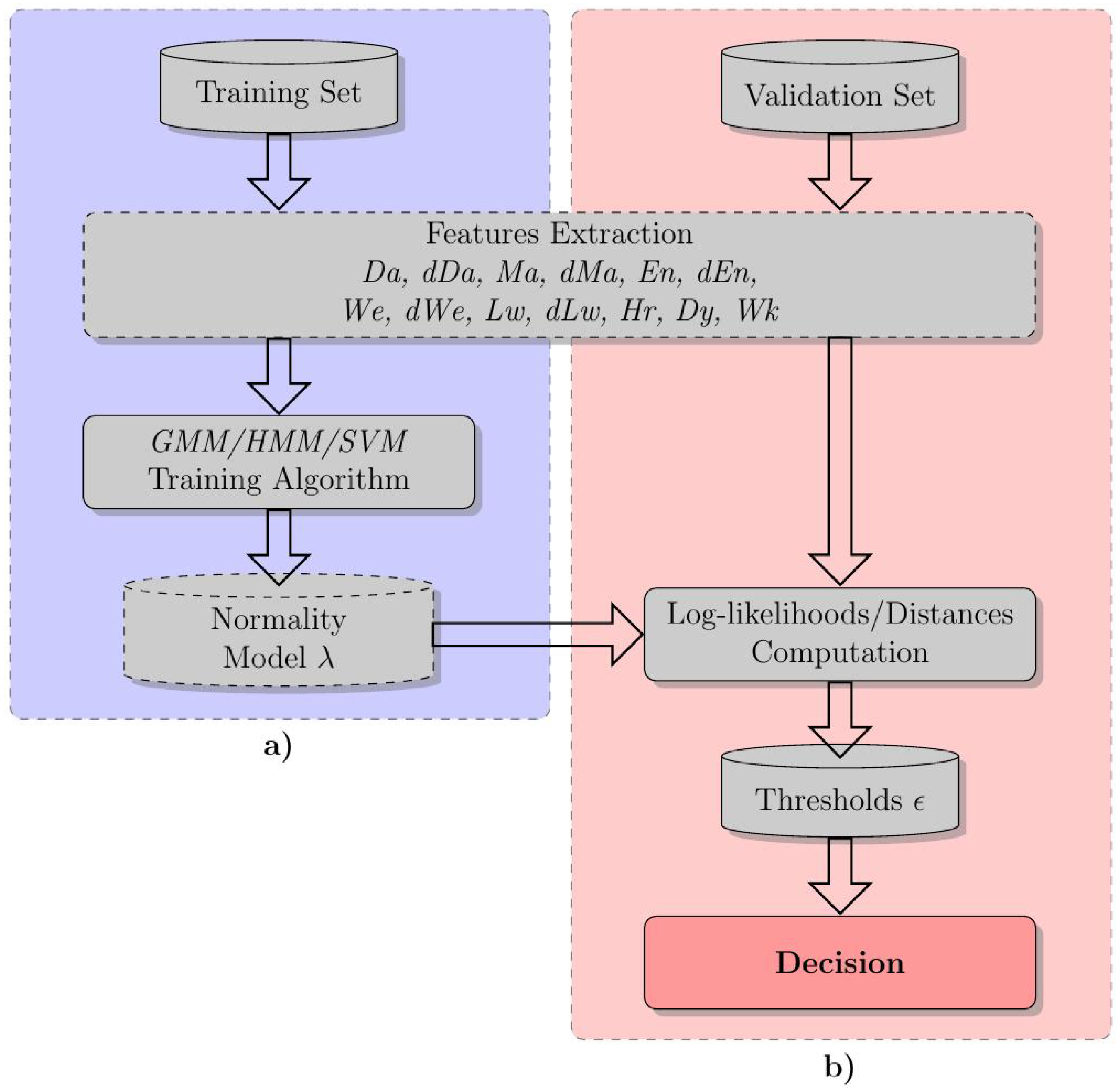
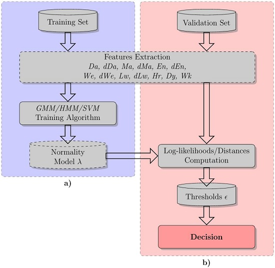
2. The Proposed Statistical Framework

The proposed framework is composed of three main parts, which are the feature extraction, the feature selection and the leakage detection. In Figure 1, the constitutive blocks for the feature extraction and the leakage detection are depicted.

As stated above, the leakage identification is based on the normality model, which captures the statistical features of the data without recorded leakages. For this reason, as shown in Figure 1, a two-stage framework has been proposed. In the normality model creation stage, the features’ information is processed to create and train the statistical model of the normal behavior. After this training phase, the models are stored to be used in the novelty detection stage. In the validation phase, all of the decisions are based on the log-likelihood values that are compared against a set of thresholds. For each frame, the corresponding log-likelihood value is obtained from the constitutive equation of the model, with the normality parameters obtained during the training phase and the new input features’ data. The set of thresholds depends on the overall log-likelihoods computed for the validation set. Being that the dataset is split into frames, the lowest resolution of the decision is represented by the frame length. For both stages, the input datasets are firstly processed in the features’ extraction block, in order to split the dataset into frames and to extract the selected features.

Three different models, extensively described in the following section, have been adopted to compute the normality model: the Gaussian Mixture Model (GMM), the Hidden Markov Model (HMM) and One-Class Support Vector Machine (OC-SVM).

The features’ selection stage operates directly on the set of extracted features based on the detection performance. For each new selected feature, the whole feature extraction and leakage detection operations are repeated. The proposed selection algorithm is extensively described in the following section.

2.1. Features

As anticipated before, a collection of both known and new features has been used to fill the gap in the literature. In particular, in order to provide a comparative evaluation, all of the suitable features available in the current literature, presented in Section 1.1, have been considered.

The energy of signals and of their wavelet decomposition sub-band, first presented in Gamboa-Medina et al. [22], have been used. Let $X=\{x_1,x_2,$ $\dots ,x_n\}$ be a vector composed of the data of the frame, with $N\in \mathbb{Z}$ samples; the energy is defined as:

$$\mathit{En}=\sum _{i=1}^N{x_i}^2.$$

(1)

Moving to the wavelet components, the decomposition of order three is performed by applying the Daubechies 2 (db2) wavelet, and overall, four sequences are obtained: three detail sequences ($D_1$,$D_2$,$D_3$) and one approximation sequence ($A_3$). For each sequence, (1) holds true, as well; thus, the energy is computed by assuming N as the number of elements in the corresponding sequence. The feature, called We, is evaluated as a vector, composed of four elements and representing the percentage of energy distribution between the wavelet components. Let $C=\left\{E{n}_{A_3},E{n}_{D_3},E{n}_{D_2},E{n}_{D_1}\right\}$ be the vector containing the computed energy for each decomposition sequence, for each j-th elements of the C; the corresponding We values is given as:

$${\mathit{We}}_j=100·\frac{C_j}{E{n}_T},$$

(2)

where $E{n}_T$ denotes the overall energy of the four components of the decomposition, given as the $L_1$ norm of C, $E{n}_T={\parallel C\parallel }_1$.

Based on this method, the authors investigated the application of the logarithm operator to the energy values of the wavelet components; thus, the j-th element of the feature Lw is defined as:

$${\mathit{Lw}}_j=log(C_j+1).$$

(3)

In order to provide a better insight into the features’ performance, the frame samples have been also adopted as a feature (Da), as well as the frame average (Ma), corresponding to the moving average of the set, for a window length equal to the frame length.

For the above features, the corresponding first order positive difference has been proposed as a feature, as well. For instance, a first order positive difference is denoted by the letter d followed by the name F of the related feature. Thus, being $F\left(n\right)$ the feature extracted from the n-th frame, the derived feature $dF$ is computed as:

$$dF\left(n\right)=\left\{\begin{array}{cc}F\left(n\right),\hfill & ifn\le 2\hfill \\ F\left(n\right)-F(n-2).\hfill & otherwise\hfill \end{array}\right.$$

(4)

where $n\in [1,Nf]$ and $Nf$ denotes the number of frames in the set. In the case of features with more components, an element-wise difference is performed. The value of two, which appears in the difference definition, is the required value that guarantees a marked dissimilarity between the frames, as well as their features, at the leakages’ beginning.

To assess the usefulness of temporal information, a set of temporal features has been evaluated. The set is composed of three features, computed for three time window lengths, respectively of one hour, one day and one week. Regarding these windows, each one is repeated over time without overlapping itself.

Regarding the temporal features, given a default sequence of temporal windows, the information regarding the belonging of the frame to a temporal window is provided as feature information. Specifically, the windows of each sequence are enumerated, and this value is assigned to the frames for which their first sample lies within the window. Therefore, according to the temporal window, the features addressed as Hr, Dy and Wk represent the hour of the day, the day of the week and the week of the year, respectively.

Except for Da and its first order positive difference (dDa), the lengths of which depend on the number of frame samples (300, 30, 10 samples at 1, 10 and 30 min of resolution, respectively), the remaining features have a fixed length, independently from dataset resolution and frame length. Specifically, Ma, En, We, Lw, Hr, Dy and Wk have a feature length of 1, 1, 4, 4, 1, 1 and 1, respectively, as summarized in

Table 2. Feature details.

Index	Name	Feature Size	Acronym
1	Data	Number of samples	Da
2	Energy	1	En
3	Moving Average	1	Ma
4	Wavelet Decomposition Energy	4	We
5	Logarithmic Wavelet Energy	4	Lw
6	Hourly Window	1	Hr
7	Daily Window	1	Dy
8	Weekly Window	1	Wk

.

2.2. GMM and HMM

Two statistical models have been chosen to characterize the normality scenario: the Gaussian mixture model and the hidden Markov model. Concerning the GMM, the creation of the background model starts by assuming a weighted combination of multivariate normal distributions (MNDs) [35]. Let ${\mathbf{x}}_{\mathbf{f}}$ be a vector of dimension L, thus a vector with L feature values, μ its mean vector and Σ its covariance matrix; the MND is defined as:

$$g\left({\mathbf{x}}_{\mathbf{f}}\right|\mathit{\mu },\mathit{\Sigma })=\frac{1}{\sqrt{{\left(2\pi \right)}^L\left|\mathit{\Sigma }\right|}}{exp}^{\left\{-\frac{1}{2}[{({\mathbf{x}}_{\mathbf{f}}-\mathit{\mu })}^T{\mathit{\Sigma }}^{-1}({\mathbf{x}}_{\mathbf{f}}-\mathit{\mu })]\right\}},$$

(5)

where $\left|\Sigma \right|$ denotes the determinant of Σ. Therefore, the GMM is obtained as an a posteriori distribution given by the weighted sum of $Ng$ instances of (5):

$$p\left({\mathbf{x}}_{\mathbf{f}}\right|\mathit{\lambda })=\sum _{g=1}^{Ng}{w}_{g}g\left({\mathbf{x}}_{\mathbf{f}}\right|{\mathit{\mu }}_g,{\mathit{\Sigma }}_g),$$

(6)

where $w_g\in [0,1]$, ${\sum }_{g=1}^{Ng}{w}_g=1$, $\lambda ={\left\{{\mu }_g,{\Sigma }_g,w_g\right\}}_{g=1}^{Ng}$ and $Ng$ denotes the number of Gaussians adopted for the GMM. The training process of the GMM follows two steps: initialization and update/finalization. In the first step, the parameters of the $Ng$ Gaussian components are computed by using the k-means algorithm; in the second step, the Expectation-Maximization (EM) algorithm [36] re-estimates the parameters, guaranteeing a monotonic increase of the likelihood and reaching its maximum value. In this study, all GMMs have a diagonal covariance matrix.

Concerning the HMM, a typical structure used in speech recognition to model the temporal processes [37] has been adopted as the second approach to characterize the background model, and it is based on the left-to-right structure (also called Bakis). Each model is characterized by a transition probability matrix $\mathbf{A}$, a sequence of emission probabilities $\mathbf{B}$, also called observation likelihoods, and a set of states $\mathbf{Q}=\left\{q_1,q_2,\dots ,q_{Ns}\right\}$. In the matrix $\mathbf{A}$, each element $a_{n,s}$ represents the probability of moving from a state n to a state s, assuming that ${\sum }_{n=1}^{Ns}{a}_{n,s}=1,\forall s$; whereas, letting $\mathbf{O}=\left\{o_1,o_2,\dots o_T\right\}$ be a given observation sequence, the generation probability of the observation $o_t$ by the state n is expressed as $b_n\left(o_t\right)$.

The Markov assumptions affirm that the probability of a particular state is dependent only on the previous state. Furthermore, the probability of an output observation $o_t$ is dependent only on the state $q_n$ that produced the observation and not on any other states or on any other observations. In this case, it is possible to compute the output likelihood, for a given model, using the iterative procedure [38]:

$$\begin{array}{ccc}& {\alpha }_1\left(n\right)=a_{0,n}{b}_n\left(o_1\right),\hfill & \hfill 1\le n\le Ns\\ & {\alpha }_t\left(n\right)=\sum _{s=1}^{Ns}{\alpha }_{t-1}\left(s\right)a_{s,n}{b}_n\left(o_t\right),\hfill & \hfill 1\le n\le Ns,1\le t\le T\\ & P\left(O\right|\lambda )={\alpha }_T\left(q_F\right)=\sum _{s=1}^{Ns}{\alpha }_T\left(s\right)a_{s,F},\hfill \end{array}$$

(7)

where $\lambda =(A,B)$ (automaton), T denotes the number of observations in $\mathbf{O}$ and $Ns$ denotes the number of states. Furthermore, $a_{0,n}$ and $a_{s,F}$ denote the transition probabilities out of the start state and into the last (or end) state, which are not associated with the observations.

In order to create a continuous density model, each observation probability distribution, $b_n\left(o_t\right)$, is represented with a mixture Gaussian density. The final model is created by adopting a special case of the EM algorithm, the forward-backward or Baum–Welch algorithm [39], which allows one to train both the transition probabilities $\mathbf{A}$ and the emission probabilities $\mathbf{B}$ of the HMM.

2.3. One-Class Support Vector Machine

As anticipated in Section 1, in addition to the backgrounds based on GMM and HMM, the experiments have been performed adopting the One-Class Support Vector Machine (SVM), as well. Generally speaking, the SVM computes a separation of the data, based on their labels, solving the following quadratic problem [40]:

$$\begin{array}{cc}\hfill \underset{w\in \mathbf{F},\xi \in {\mathbb{R}}^l,\rho \in \mathbb{R}}{min}& \frac{1}{2}{\parallel w\parallel }^2+\frac{1}{vl}\sum _i{\xi }_i-\rho ,\hfill \\ \hfill \text{subject}\text{to}& (w·\mathrm{\Phi }\left({\mathbf{x}}_{\mathbf{i}}\right))\ge \rho -{\xi }_i,{\xi }_i\ge 0,\hfill \end{array}$$

(8)

to obtain the decision function:

$$f\left({\mathbf{x}}_{\mathbf{f}}\right)=\mathrm{sgn}\left(\sum _i{\alpha }_i·k({\mathbf{x}}_{\mathbf{i}},{\mathbf{x}}_{\mathbf{f}})-\rho \right),$$

(9)

where ${\mathbf{x}}_{\mathbf{i}}$ denotes the i-th Support Vector (SV) and $k(·,·)$ represents the Gaussian kernel, defined as $k(\mathbf{x},\mathbf{y})=exp(-{\parallel \mathbf{x}-\mathbf{y}\parallel }^2/c)$.

The function f returns $+1$ in the “small” region where most of the data points fall and $-1$ everywhere else. The strategy is to map the data into a features space corresponding to the kernel and to separate the data from the origin with the maximum margin. For a new point ${\mathbf{x}}_{\mathbf{f}}$, the value of $f\left({\mathbf{x}}_{\mathbf{f}}\right)$ is determined by evaluating on which side of the hyperplane of the features space ${\mathbf{x}}_{\mathbf{f}}$ falls.

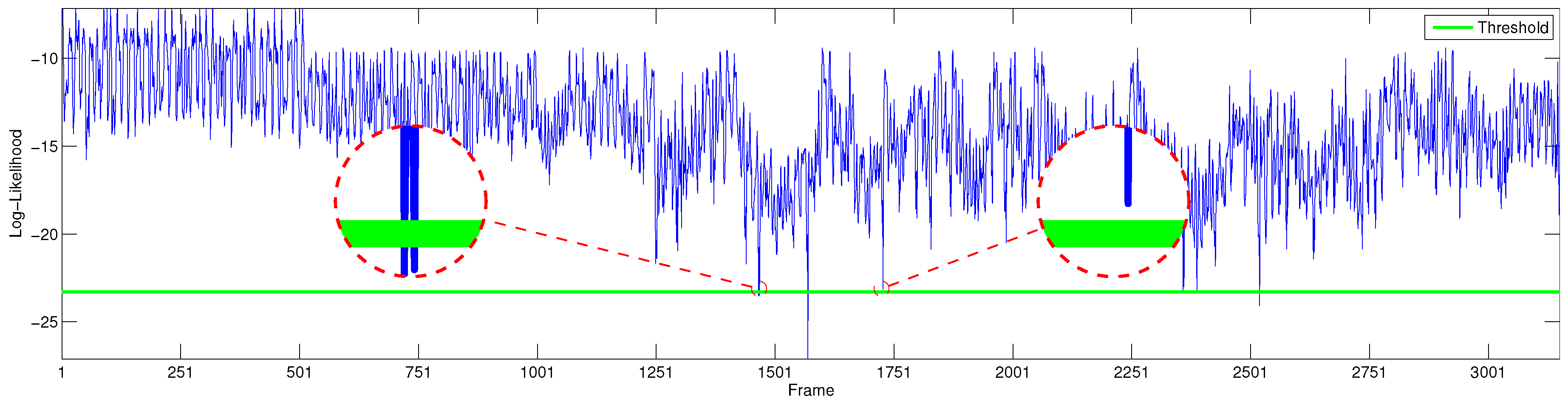
2.4. Novelty Detection

The decision stage, which carries out the detection of an event as being normal or abnormal, is depicted in the novelty detection stage in Figure 1, and is composed of four blocks, strictly interconnected among themselves: normality model λ, log-likelihood computation, threshold ϵ and decision. For each frame, in the GMM approach, or for each sequence of frames, in the observation sequence for the HMM approach, the vector of extracted features is used to compute the corresponding log-likelihood value, by means of Equation (6) or (7), respectively, and by adopting the trained parameters of the background model.

At first, the validation data are processed and the achieved log-likelihoods stored. Then, a set of thresholds, to compare against the achieved log-likelihoods, is computed, and a non-uniform distribution of the threshold values is adopted, by arranging a higher number of thresholds, wherever the log-likelihood presents a denser distribution. In the decision block, each threshold is compared against the log-likelihoods computed for the frame (GMM case) or the sequence of frames (HMM case). As depicted in Figure 2, if the log-likelihood value exceeds the threshold, the event is marked as a leakage/abnormal event, otherwise it is considered a normal event. Being that the HMM is based on a sequence of observations, consecutive frames are dragged in the decision process. In particular, the number of frames, involved in the observation, is equal to the number of states assumed for the normality background. Since the value of the likelihood returned by the algorithm is a logarithm, the data that match the statistical model will produce a probability value close to one, which corresponds to a value close to zero to the logarithm. On the other hand, the data not matching the statistical model will generate a probability value close to zero; thus, the logarithm value will be negative, while its absolute value will be great, as shown in Figure 2.

With respect to the block diagram Figure 1, the adoption of the SVM affects the novelty detection stage. Instead of using the log-likelihood values returned by the GMM or HMM, the decision is based on the distances of each frame from the separation hyperplane of the feature points, obtained during the training phase. The set of thresholds used in the validation process is chosen consequently.

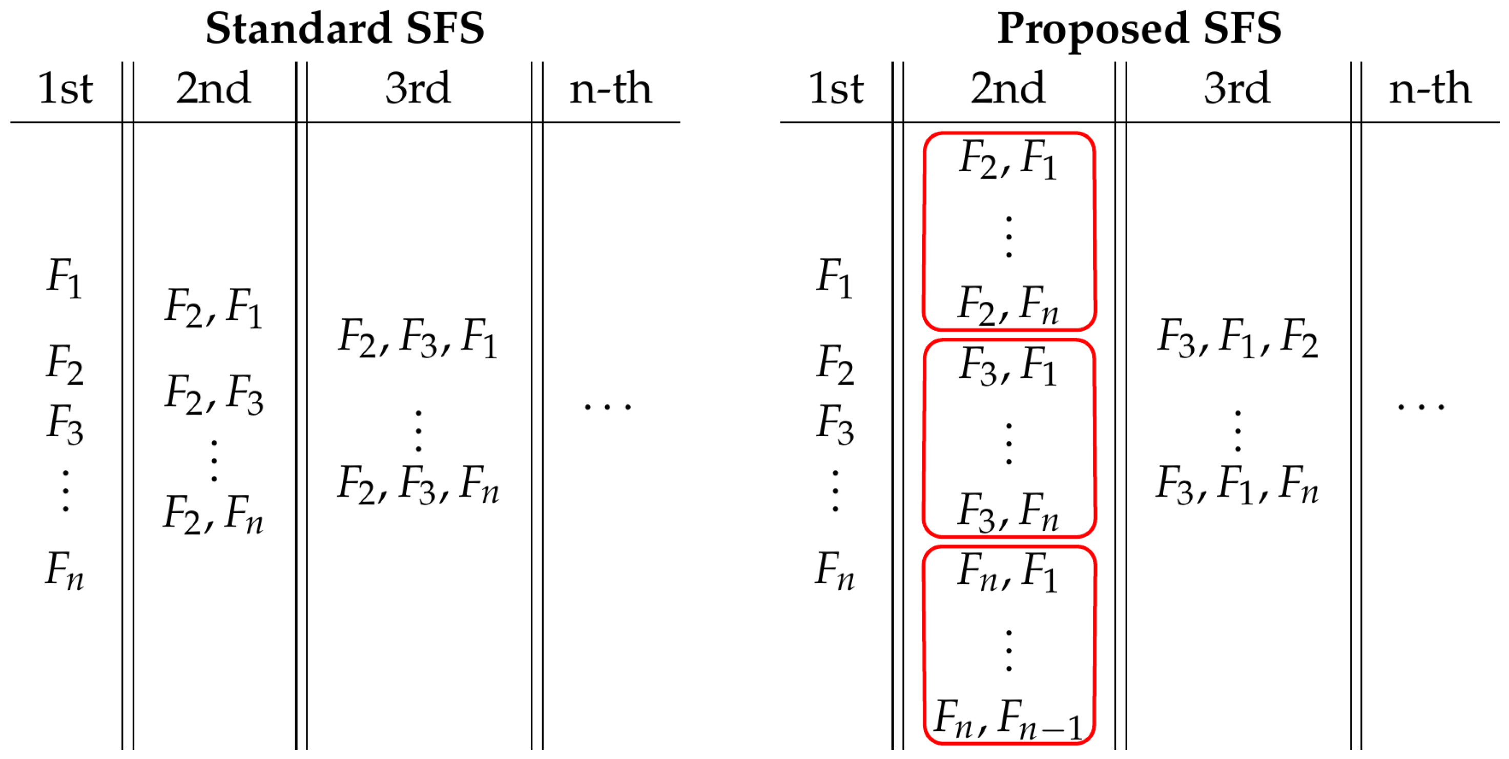
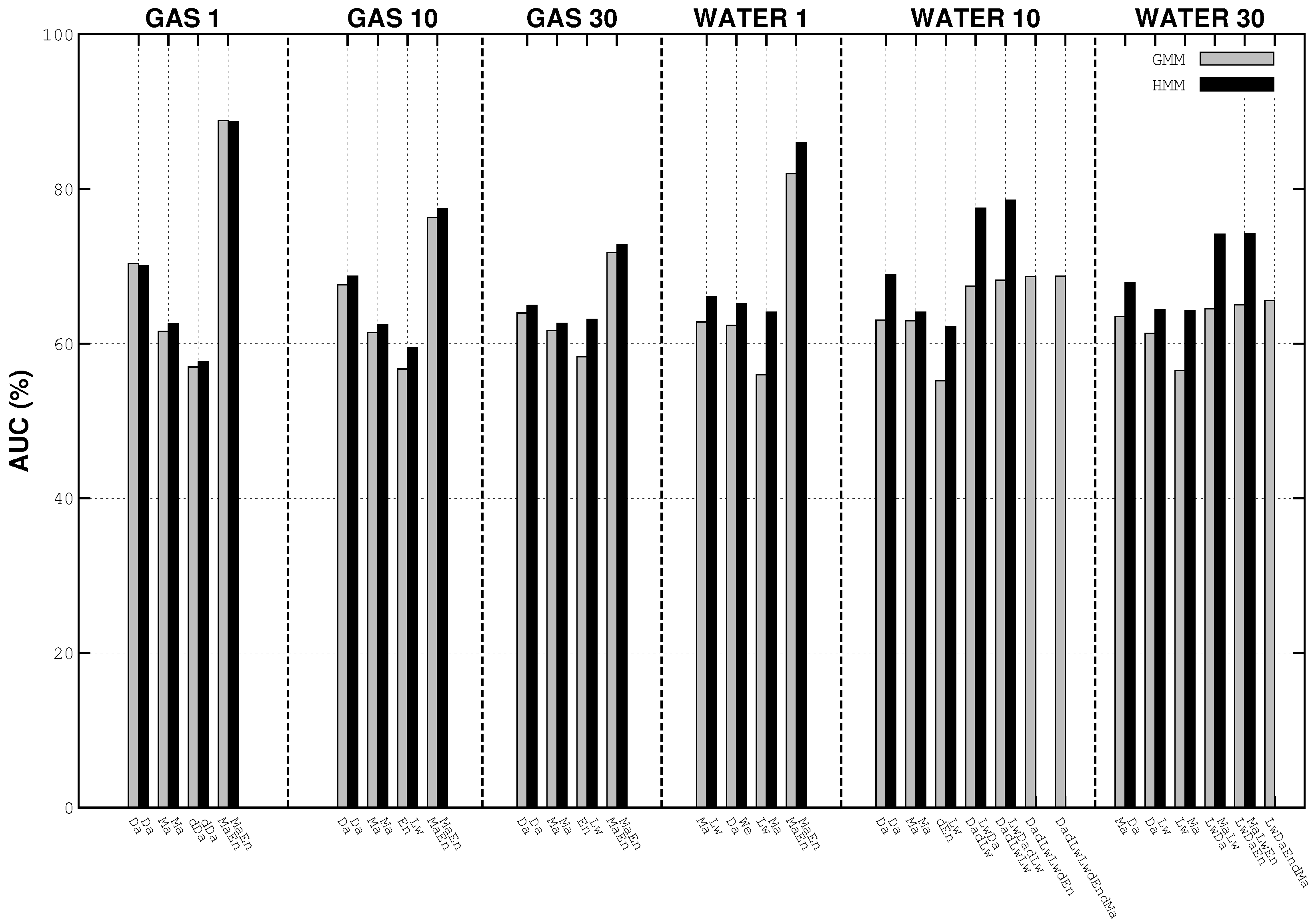
2.5. Feature Selection

As anticipated in Section 2.1, in the literature, a well-defined set of standard features is yet to be defined. Furthermore, an exhaustive research requires testing a number of combinations that can be computed as the binomial coefficient: $m!/l!(m-l)!$, where m denotes the number of available features and l the features for each vector combination. In other words, the overall number of combinations is given as ${\sum }_{l=1}^{m}m!/l!(m-l)!$, with $m=10$, for a total of 1023 combinations, meaning that an investigation of all of the possible combinations is unaffordable from a computational standpoint. To overcome this issue, a modified version of the Sequential Forward Selection (SFS) algorithm [33] has been adopted to perform the feature selection.

The SFS is a suboptimal method that allows reducing the number of tested combinations to $lm-l(l-1)/2$, by lowering the overall number of combinations to ${\sum }_{l=1}^{m}lm-l(l-1)/2=m(m+1)/2$. For instance, given $m=10$ available features, a total of 55 combinations is tested by means of the SFS, against the 1023 of the full-search.

The SFS consists of l sequential steps; in each step, a winning combination of features is selected from a pool of features, and with respect to the previous step, the number of features in the winning combination is increased by one, removing the selected feature from the pool. Further details on the SFS algorithm are described in Algorithm 1, where the Area Under the Curve (AUC) has been used as the criterion value.

Algorithm 1 Sequential forward selection.

1: procedure Initialization 2:     - Create a set of m feature vectors, each composed of a single feature. 3: end procedure 4: procedure Combination 5:     for $i=1\to (m-1)$ do 6:         - Compute the criterion value for each vector of the set. 7:         - Select the winner vector, i.e., the one whose criterion value is greatest. 8:         - Create a new set of $m-i$ feature vectors, each of them composed of 9:          the winning vector and one of the excluded features. 10:     end for 11: end procedure 12: - Select the feature vector whose criterion value is greatest among all of the created feature vectors.

As depicted in Figure 3 and Figure 4, the low performance achieved in the first iteration, in particular with the GMM, has suggested that the chances of missing a good combination are considerably high; this is the reason why a slight variation in the first and the second step of the SFS algorithm has been introduced.

In our implementation of the SFS algorithm, as shown in Figure 5, at the first step, instead of choosing a single winner, three winners are selected, that is the three features that have the best results. Then, in the second step, for each winner, a new features set, as reported in Algorithm 1, is created and tested. Among all of these sets, the winner to be used in the next step is selected, and the SFS default procedure is followed from now on. While improving the search performance, the proposed selection method remains a suboptimal search approach, keeping an overall number of required iterations, 73 for $m=10$, still lower than an exhaustive search.

3. Experiments

In this section, an overview of the general setup is presented, describing the adopted datasets and the basic parameters used for each approach introduced in Section 2.

3.1. Datasets

As highlighted by Fagiani et al. [2], only a few datasets exist that are publicly available while having proper data to perform experiments. Considering the residential scenario, the only available dataset is the Almanac of Minutely Power dataset (AMPds) [29]. It is composed of 2 full years worth of recordings, at 1-min intervals, of electricity, water and natural gas consumption of a single house. For larger grids, a valid candidate that includes both water and natural gas recordings is the dataset of monthly consumption, released in the “live data page for energy and water consumption” of the Department of International Development [30]. The records report the energy, natural gas and water consumption of the headquarters and Abercrombie House buildings. Each DFID subset has a sampling time of 30 min, and the last data that have been recorded date back to 31 March 2015. Two subsets report gas consumption values, specifically the overall DFID and the Abercrombie House sets; whereas the water consumption values are reported in the Abercrombie House and Whitehall sets. Moreover, the records for the Abercrombie House water and gas sets started on 8 August 2013 and 28 July 2010, respectively; on 1 August 2010, for the overall gas set, and on 20 April 2013, for the Whitehall set. Therefore, concerning the residential scenario, AMPds, three data resolutions have been exploited, i.e., the original one, 1 min, then a lower resolution of 10 min and, finally, a 30-min one, not presented in the previous work [13]. For the building scenario, only the original DFID resolution of 30 min has been exploited. Furthermore, it should be noted that a further resolution reduction would lower the number of records in the dataset too much to be of use.

3.2. Computer Simulation Setup

The datasets have been split into two parts; $70\%$ of the data are used for training purposes (background model creation), and the remaining $30\%$ is used for testing (detection performance evaluation). Furthermore, each subset has been split in overlapping frames with a fixed length of 5 h, thus 300 samples at 1-min resolution, 30 samples at 10 min and 10 samples at 30 min. The overlap is equal to $2/3$ of the frame length. A label vector has been created for the validations set, by marking with “0” (zero) the normal frames, and “1” (one) the abnormal ones.

The background model creation includes an initial random condition, which can cause slight changes in the model from one run to another. Therefore, based on the same training set, 10 background models have been created. Each model has been adopted to evaluate 10 leakages, the parameters of which are randomly selected.

The GMMs have been tested by varying the number of adopted Gaussian components as: $N_g=\left\{2,4,8,16,32,64,128,256\right\}$. For the HMMs, in addition to the Gaussian components, the number of states has been varied as well, from one to four (plus the start and end states, which are always present). For the OC-SVM only, the γ parameter has been varied based on the following pool of values: $\left\{2^{-15},2^{-13},\dots 2,2^3\right\}$.

The data preparation, the feature extraction and the decision stages have been developed in MATLAB^®: MathWorks, Natick, MA, USA. The GMM and HMM training algorithms, as well as the likelihood computation, have been implemented in C++ using the Torch3 library [41]. The OC-SVM has been implemented using the LIBSVM library [42].

In order to produce reliable and consistent results, improvements have been applied to the experimental setup with respect to the one presented in [13]. The random leakages parameters have been produced by initializing the MATLAB^® random generator with the seed of 42. Moreover, the min-max normalization has been also applied to each feature set. In particular, let ${\mathbf{x}}_{\mathbf{f}}$ be the feature set for each frame; the corresponding normalized set ${{\mathbf{x}}_{\mathbf{f}}}^{*}\in {[0,1]}^L$, with L denoting the number of elements in the vector ${\mathbf{x}}_{\mathbf{f}}$, is given performing the following element-wise operation:

$${{\mathbf{x}}_{\mathbf{f}}}^{*}=\frac{{\mathbf{x}}_{\mathbf{f}}-{{\mathbf{x}}_{\mathbf{f}}}^m}{{{\mathbf{x}}_{\mathbf{f}}}^M-{{\mathbf{x}}_{\mathbf{f}}}^m},$$

(10)

where ${{\mathbf{x}}_{\mathbf{f}}}^M$ and ${{\mathbf{x}}_{\mathbf{f}}}^m$ denote the vectors of maximum and minimum values, respectively. For each component of ${\mathbf{x}}_{\mathbf{f}}$, the maximum and the minimum values are computed from the training set.

3.3. Leakage Creation

As discussed in Section 1, in the novelty detection approach, no faulty instance is adopted to train the normality model, and none is present in the datasets. As said, also, to the authors’ knowledge [2], in addition to the suitable datasets being limited in number, none of them records the occurrence of faults. Therefore, the validation datasets have been manipulated to include faulty instances and to perform the validation of the system. Each validation sequence has been revised as:

$$v\left(i_v\right)=\left\{\begin{array}{cc}v\left(i_v\right)+\beta ·l_k,\hfill & if{i_v}^{\left(i\right)}\ge n\ge {i_v}^{\left(f\right)}\hfill \\ v\left(i_v\right),\hfill & otherwise\hfill \end{array}\right.$$

(11)

where $\beta \in [0.25,0.50]$, $l_k$ is the average consumption computed from the training sequence, while ${i_v}^{\left(i\right)}$ and ${i_v}^{\left(f\right)}$ denote the leakage start and stop samples. The leakage duration is randomly selected in a range between a min of 5 and a max of 10 h, which corresponds to 300 and 600 samples, respectively, for 1-min resolution, to 30 and 60 samples, respectively, for 10-min resolution, and 10 and 20 samples, respectively, for 30-min resolution. Furthermore, the starting point of the leakage is randomly selected over a span between the $10\%$ and $90\%$ of the validation set length. An example of leakage induced in the data, together with a subset of features extracted from the corresponding data, is shown in Figure 6.

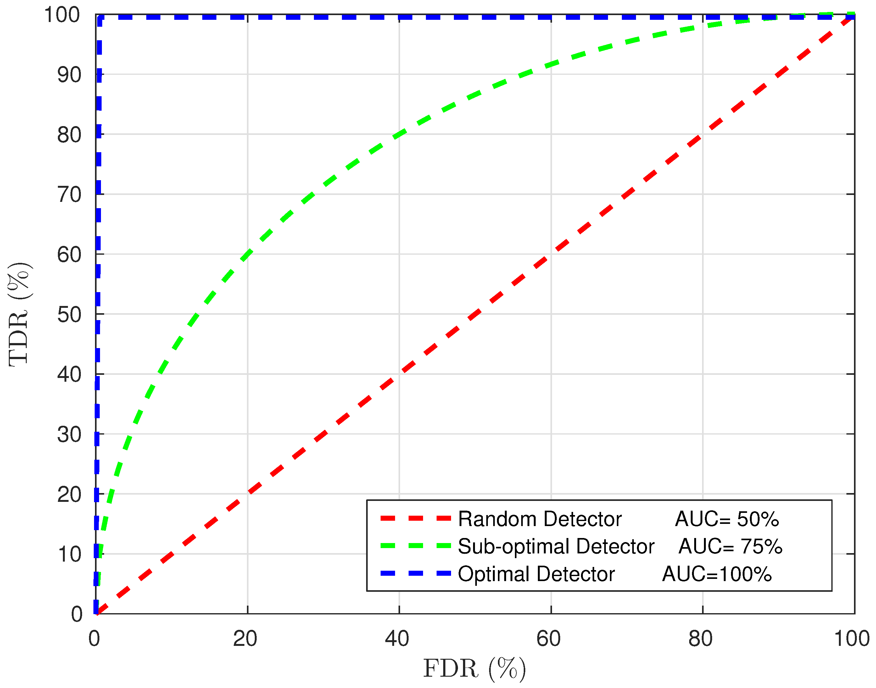
3.4. Evaluation Method

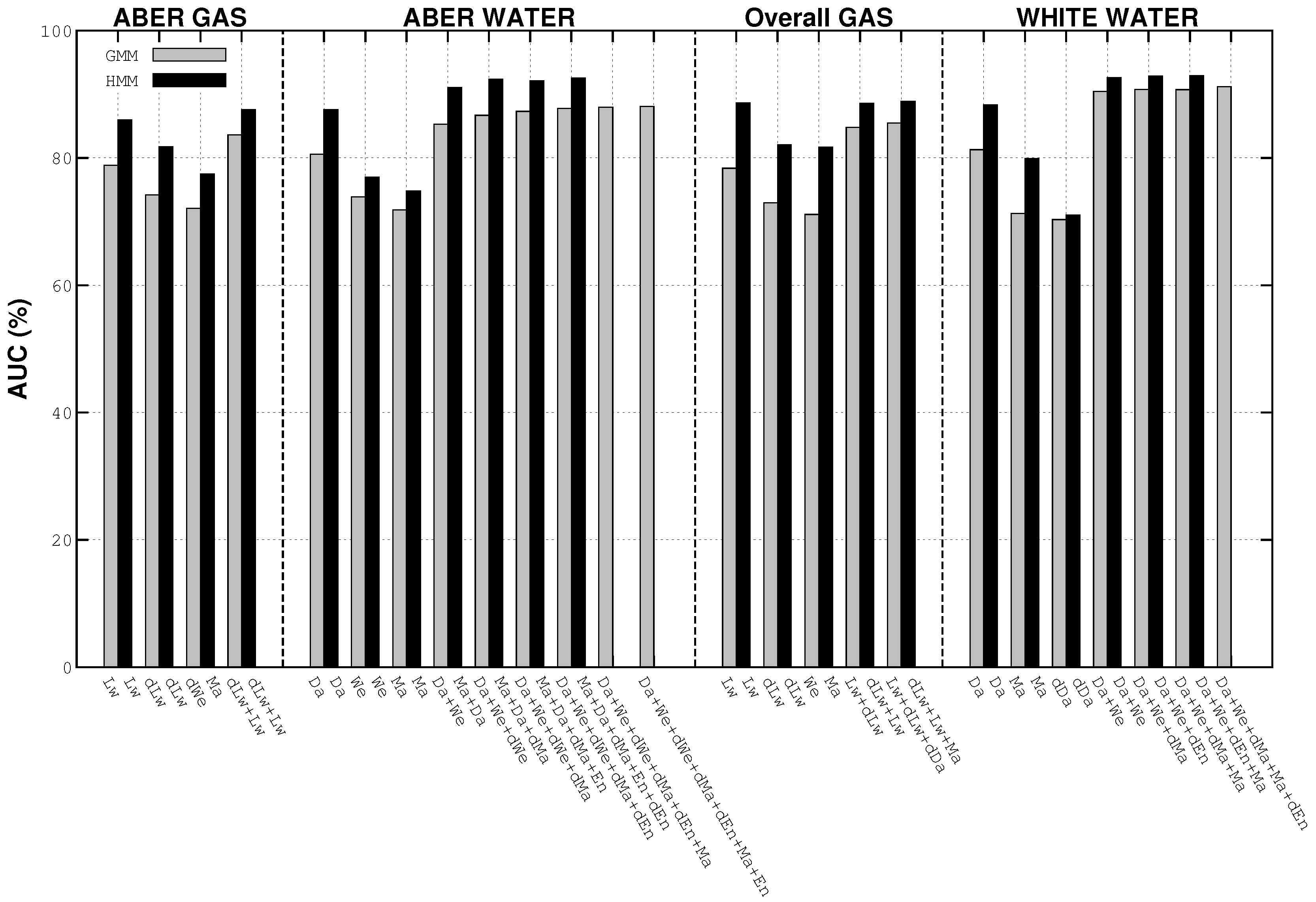
In order to evaluate the performance of the system, the probability to correctly detect an anomaly, TDR, and the probability to erroneously detecting an anomaly, FDR, have been adopted and are given, according to Ntalampiras et al. [43], as follows:

$$\begin{array}{cc}\hfill TDR=& \frac{no.ofabnormaleventsdetectedasabnormal}{no.ofabnormalevents},\hfill \\ \hfill FDR=& \frac{no.ofnormaleventsdetectedasabnormal}{no.ofnormalevents}.\hfill \end{array}$$

(12)

Assuming a set of thresholds, for each threshold, the corresponding TDRs and FDRs are obtained, and these values are used to plot the Receiver Operating Characteristic (ROC) curve [44], which shows how the threshold affects the result.

On the one hand, if the threshold is set to a value lower than the minimum likelihood, the system achieves a TDR and an FDR equal to $0\%$. Each normal event is correctly detected, but all of the abnormal events are classified as normal, as well. On the other hand, if the threshold is set to a value higher than the maximum likelihood, both the TDR and the FDR reach a $100\%$ rate. In the latter case, then, each sequence is recognized always as abnormal notwithstanding its actual nature.

As the last step, for a given ROC, the goodness of the classifier performance is evaluated in terms of AUC, as done in [31,32,43]. Specifically, the plot relating to a random guess detector and an ideal detector is reported, as a reference, in Figure 7. It is possible to observe that a completely random guess will produce a set of points along the diagonal of the ROC, producing an AUC of $50\%$. On the other hand, the optimal detector will produce a $100\%$ AUC, and the best threshold will be the one that produces a TDR of $100\%$ and a FDR of $0\%$. Thus, a novelty detector, to be of particular use, should have a plot above the diagonal of the ROC. Furthermore, the closer to the top-left corner of the ROC, the better the detector performance will be.

4. Results

The results achieved by each approach, based on the proposed SFS procedure, with and without temporal features, are presented and discussed in this section. The best AUC results, achieved for the residential consumption and, thus, based on the AMPds datasets are reported in

Table 3. Best results and corresponding features’ combination achieved for each resource and resolution (Res.) of the AMPds dataset. The column “Parameters” reports the number of Gaussians, the states and Gaussians number and the γ value for GMM, HMM and One-Class (OC)-SVM, respectively.

Resource	Res.	AUC (%)	SD	Model	Parameters	Features Combination
Without Temporal Features
Gas	1	$88.82$	$9.83$	GMM	256	Ma + En
Gas	1	$88.68$	$9.72$	HMM	1–256	Ma + En
Gas	1	$54.97$	$19.27$	OC-SVM	$2^3$	dWe + We
Gas	10	$76.33$	$14.07$	GMM	128	Ma + En
Gas	10	$77.45$	$15.56$	HMM	3–256	Ma + En
Gas	10	$57.29$	$17.55$	OC-SVM	2	dWe + dLw
Gas	30	$71.75$	$15.03$	GMM	128	Ma + En
Gas	30	$72.76$	$17.13$	HMM	3–256	Ma + En
Gas	30	$60.11$	$15.65$	OC-SVM	2	dWe + dLw
With Temporal Features
Gas	1	$88.78$	$9.84$	GMM	256	Ma + En
Gas	1	$88.85$	$9.69$	HMM	3–256	Ma + En
Gas	1	$54.97$	$19.27$	OC-SVM	$2^3$	dWe + We
Gas	10	$76.35$	$14.48$	GMM	256	Ma + En
Gas	10	$77.50$	$15.54$	HMM	3–256	Ma + En
Gas	10	$57.29$	$17.55$	OC-SVM	2	dWe + dLw
Gas	30	$71.83$	$15.49$	GMM	256	En + Ma
Gas	30	$72.83$	$17.19$	HMM	3–256	Ma + En
Gas	30	$60.11$	$16.65$	OC-SVM	2	dWe + dLw

and

Table 4. Best results and corresponding features’ combination achieved for each resource and resolution (Res.) of the Almanac of Minutely Power dataset (AMPds) dataset. The column “Parameters” reports the number of Gaussians, the states and Gaussians number and the γ value for GMM, HMM and One-Class (OC)-SVM, respectively.

Resource	Res.	AUC (%)	SD	Model	Parameters	Features Combination
Without Temporal Features
Water	1	$81.94$	$10.21$	GMM	128	Ma + En
Water	1	$86.36$	$10.54$	HMM	4–64	Ma + En
Water	1	$54.50$	$16.66$	OC-SVM	$2^3$	dWe + dEn
Water	10	$68.70$	$12.83$	GMM	256	Da + dLw + Lw + dEn + dMa
Water	10	$78.55$	$14.98$	HMM	4–256	Lw + Da + dLw
Water	10	$62.90$	$14.30$	OC-SVM	$2^3$	dWe + dEn
Water	30	$66.94$	$15.29$	GMM	256	Lw + Ma + En + dMa + dLw + Da + dEn
Water	30	$74.21$	$17.79$	HMM	4–256	Ma + Lw + En
Water	30	$65.48$	$12.24$	OC-SVM	$2^3$	We + dEn
With Temporal Features
Water	1	$81.94$	$10.07$	GMM	128	Ma + En
Water	1	$86.55$	$10.51$	HMM	4–64	Ma + En
Water	1	$54.50$	$16.66$	OC-SVM	$2^3$	dWe + dEn
Water	10	$70.60$	$16.13$	GMM	256	Ma + Hr + dMa
Water	10	$80.21$	$15.13$	HMM	4–256	Lw + Da + Hr + dLw + Wk + Ma + dEn
Water	10	$62.90$	$14.30$	OC-SVM	$2^3$	dWe + dEn
Water	30	$71.90$	$13.91$	GMM	256	Da + Hr + dEn + dMa + En + Ma
Water	30	$80.07$	$13.07$	HMM	4–256	Da + Hr
Water	30	$65.48$	$12.24$	OC-SVM	$2^3$	dWe + dEn

, whereas the results achieved for the building consumption, based on the DFID dataset, are reported in

Table 5. Best results and corresponding features’ combination achieved for each resource and resolution (Res.) of the Department of International Development (DFID) dataset. The Abercrombie and the Whitehall sets are reported as “Aber.” and “White.”, respectively. The column “Parameters” reports the number of Gaussians, the states and Gaussians number and the γ value for GMM, HMM and One-Class (OC)-SVM, respectively.

Resource	Res.	AUC (%)	SD	Model	Parameters	Features Combination
Without Temporal Features
Aber. Gas	30	$83.61$	$9.30$	GMM	256	dLw + Lw
Aber. Gas	30	$87.59$	$10.15$	HMM	4–64	dLw + Lw
Aber. Gas	30	$75.30$	$25.91$	OC-SVM	$2^{-7}$	Da + dMa + Ma + En
Aber. Water	30	$87.77$	$5.93$	GMM	256	Da + We + dWe + dMa + dEn
Aber. Water	30	$92.52$	$5.58$	HMM	3–256	Ma + Da + dMa + En + dEn
Aber. Water	30	$67.06$	$33.50$	OC-SVM	$2^{-7}$	Da + Ma + En
Overall Gas	30	$85.47$	$10.85$	GMM	256	Lw + dLw + dMa
Overall Gas	30	$88.85$	$11.22$	HMM	4–256	dLw + Lw + Ma
Overall Gas	30	$79.56$	$23.95$	OC-SVM	$2^{-3}$	Da + dDa + dMa + dEn
White. Water	30	$91.21$	$5.83$	GMM	256	Da + We + dMa + Ma + dEn
White. Water	30	$92.88$	$4.53$	HMM	4–128	Da + We + dEn + Ma
White. Water	30	$65.39$	$39.03$	OC-SVM	$2^{-5}$	Da + Ma
With Temporal Features
Aber. Gas	30	$85.00$	$10.29$	GMM	256	Lw + dLw + Hr + Ma
Aber. Gas	30	$87.80$	$10.55$	HMM	4-256	dLw + Lw + Hr + Wk + Ma
Aber. Gas	30	$75.35$	$25.91$	OC-SVM	$2^{-7}$	Da + dMa + Ma + En
Aber. Water	30	$90.07$	$6.64$	GMM	256	Da + Hr + We + dWe + Ma + dEn + dMa
Aber. Water	30	$94.73$	$5.62$	HMM	4–256	Da + Hr + Ma + dMa
Aber. Water	30	$67.06$	$33.56$	OC-SVM	$2^{-7}$	Da + Ma + En
Overall Gas	30	$86.60$	$10.63$	GMM	256	dLw + Lw + Hr + dMa + Ma
Overall Gas	30	$89.56$	$12.04$	HMM	4–32	Lw + dLw + dMa + Wk + Dy + Ma
Overall Gas	30	$79.56$	$33.56$	OC-SVM	$2^{-7}$	Da + Ma + En
White. Water	30	$93.65$	$6.74$	GMM	256	Da + Hr + Dy
White. Water	30	$95.32$	$5.67$	HMM	2–256	Da + Hr + Dy + dEn
White. Water	30	$65.39$	$39.03$	OC-SVM	$2^{-5}$	Da + Ma

. In Figure 3 and Figure 4, for each dataset and resolution, the AUCs achieved by the winners of each selection step of the proposed SFS process, with both GMM and HMM, but without temporal features, are reported.

4.1. Residential Consumption

In the residential scenario, the best results are achieved, for almost every resolution level and resource type, by the HMM models, although with a higher standard deviation with respect to the results of the GMM models. The only exception is the case of natural gas at 1-min time resolution without temporal features, in which the GMM models outperform the HMM counterpart. The SVM performance is significantly worse than the GMM and HMM ones.

Regarding the features, it can be observed that, in the case of the gas results, the moving average, Ma, and the energy, En, features are always present, in both the GMM and HMM evaluations, and they seem to be a suitable set of features for the natural gas leakage detection. The temporal features do not provide a boost in performance. The overall best results for GMM and HMM, $88.82\%$ and $88.68\%$, respectively, are achieved at 1-min resolution.

In the case of water records, HMM achieved the best performance notwithstanding the time resolution, although the best overall results, $86.36\%$, are obtained at 1-min time resolution. Moreover, the introduction of the temporal information has led to a performance improvement at 10 and 30 min of resolution with both GMM and HMM. Concerning GMM, the improvements are about $1.9\%$ and $4.96\%$, for 10 and 30 min, respectively. In the case of HMM, at the same time resolutions, the respective improvements are about $1.66\%$ and $5.86\%$.

In the water case, also, longer features’ combinations have been obtained, especially at 10 and 30 min of resolution, and it is difficult to identify common features’ combinations. Concerning the temporal features, in the GMM case, the only temporal feature is the one obtained with the hourly window, Hr. In the case of HMM, at 10 min, two temporal features are present, hourly and weekly, whereas at 30 min, only the hourly one is present.

It is noteworthy that, with both water and natural gas data, decreasing the resolution produces worse results with both GMM and HMM models, whereas the opposite trend is shown by SVM.

It should be noted that to apply novelty detection to metering systems based on low power devices, in the natural gas case, suitable performance levels are achieved only at 1-min resolution, whereas in the water case, valuable results have been obtained at every resolution value. With respect to the computational burden, on the other hand, in the gas case, the GMM model achieves performance close to the HMM one at all resolutions; therefore, the high computational burden due to the sampling rate can be partially lowered by choosing the GMM model instead of the HMM one. On the other hand, in the water case, the temporal features at 30-min resolution allow one to further reduce the computational burden of the system. Specifically, the features’ vector Ma+Lw + En turns into Da + Hr, thus losing the heavy computation required by the wavelet decomposition. Thus, if the aim is to implement the algorithm on a concentrator or similar low power computation devices, there is room to optimize the procedure with little to no loss in terms of performance.

4.2. Building Consumption

In the case of the building scenario, the best performance is achieved by the HMM model notwithstanding the time resolution of the samples. SVM in this case, as well, results in being the worst performer. The introduction of temporal features has provided additional performance improvement to both the GMM and HMM models, whereas SVM has not shown significant gain.

About the Abercrombie gas subset, the best result, $87.80\%$, is achieved by the HMM model, introducing the hourly and weekly temporal features, and the performance improvement is about $1.39\%$ and $0.21\%$ for GMM and HMM, respectively.

Concerning the Abercrombie water set, $2.30\%$ and $2.21\%$ of improvements are obtained by introducing the temporal features. Specifically, the HMM best result, $94.73\%$, is achieved by adopting the daily temporal feature.

The best result performed with the overall gas set is $89.24\%$, by introducing both the daily and the weekly temporal features, and obtaining enhancements of $1.13\%$ and $0.71\%$ for GMM and HMM, respectively.

In the case of the Whitehall set, the introduction of temporal features produced an improvement of $2.44\%$ for both GMM and HMM. The best result is $95.32\%$, and the improvements are achieved by introducing the hourly and the daily features for both GMM and HMM.

The results of the experiments show that the proposed solution is compatible with low power metering devices, and the data precessing may also be suitable for low power computational devices. Specifically, for some scenarios, the application of temporal features, together with the general performance improvement, allows one to reduce the computational burden by effecting the features’ combinations. In the case of HMM model, the features’ set obtained for the Abercrombie water data is reduced from Ma + Da + dMa + En + dEn to Da + Hr + Ma + dMa; thus from five to four features and from 14 to 13 overall components. Whereas, for the White water set, the features go from Da + We + dEn + Ma to Da + Hr + Dy + dEn, thus removing the need for the heavy computational power required for the wavelet decomposition. On the other hand, in the case of the GMM model, for the White water data, the features set Da + We + dMa + Ma + dEn is reduced to Da + Hr + Dy, going from five to three features and from 14 to 12 overall components.

4.3. Best Results’ Details

In order to have a better insight into the detection performance for the best results, in

Table 6. Best results’ details. TDR, True Detection Rate; FDR, False Detection Rate; BG, Background. The Whitehall set is reported as “White.”.

Resource	AUC (%)			TDR (%)	FDR (%)
	AVG	BEST BG	BEST		AVG	BEST BG	BEST
AMPds Gas	$88.82$	$93.{27}_{\left(6\right)}$	$99.{84}_{(5/3)}$	100	$25.32$	$14.65$	$0.26$
AMPds Water	$86.36$	$91.{46}_{\left(8\right)}$	$99.{76}_{(7/6)}$	100	$29.43$	$22.33$	$0.57$
Overall Gas	$89.56$	$94.{68}_{\left(8\right)}$	$99.{99}_{(3/5)}$	100	$18.17$	$10.26$	$0.02$
White. Water	$95.32$	$96.{97}_{\left(8\right)}$	$99.{97}_{(10/9)}$	100	$9.36$	$6.14$	$0.06$

, together with the best results achieved (column “AVG”), are also reported the best AUCs achieved among the background models (column “BEST BG”), and the overall best AUC (column “BEST”). The former refers to the best result achieved as the average of the AUC results, obtained for all of the tested leakages with the same background model. The latter shows the best AUC achieved among the detected leakages, regardless of the adopted background model. As discussed in Section 3.2, for each experiment, 10 background models are trained, and for each of them, 10 random leakages are tested. Therefore, the background number, for the “BEST BG”, and the background and the leakage number, for the “BEST”, that have achieved the reported result, are indicated in brackets. The ROCs concerning the average AUCs achieved for each background model, among all of the tested leakages and the overall averages, are depicted in Figure 8.

Furthermore, also the TDRs and FDRs are reported in Table 6. The values are obtained from the corresponding ROCs. Each FDR has been computed for the lowest likelihood value that achieves a TDR of $100\%$. Note that the FDRs reported in Table 6 cannot be compared to the points for the TDRs of $100\%$ in the curves depicted in Figure 8. Differently from the ROCs, where the average curves have been computed considering both TDR and FDR points, the results in Table 6 have been achieved performing the average of the FDR components only.

Finally, in order to validate the best results and to provide a hint of the general performance, the k-fold cross-validation, with $k=8$, has been executed. The proposed SFS has been repeated in the k-fold perspective, by considering the water and natural gas residential consumption, the AMPds dataset, at 1 min of resolution using the GMM model. For both natural gas and water, the best result, $92.00\%$ and $84.62\%$, respectively, has been achieved by the combination of Ma and En features, confirming the results reported in Table 3 and Table 4.

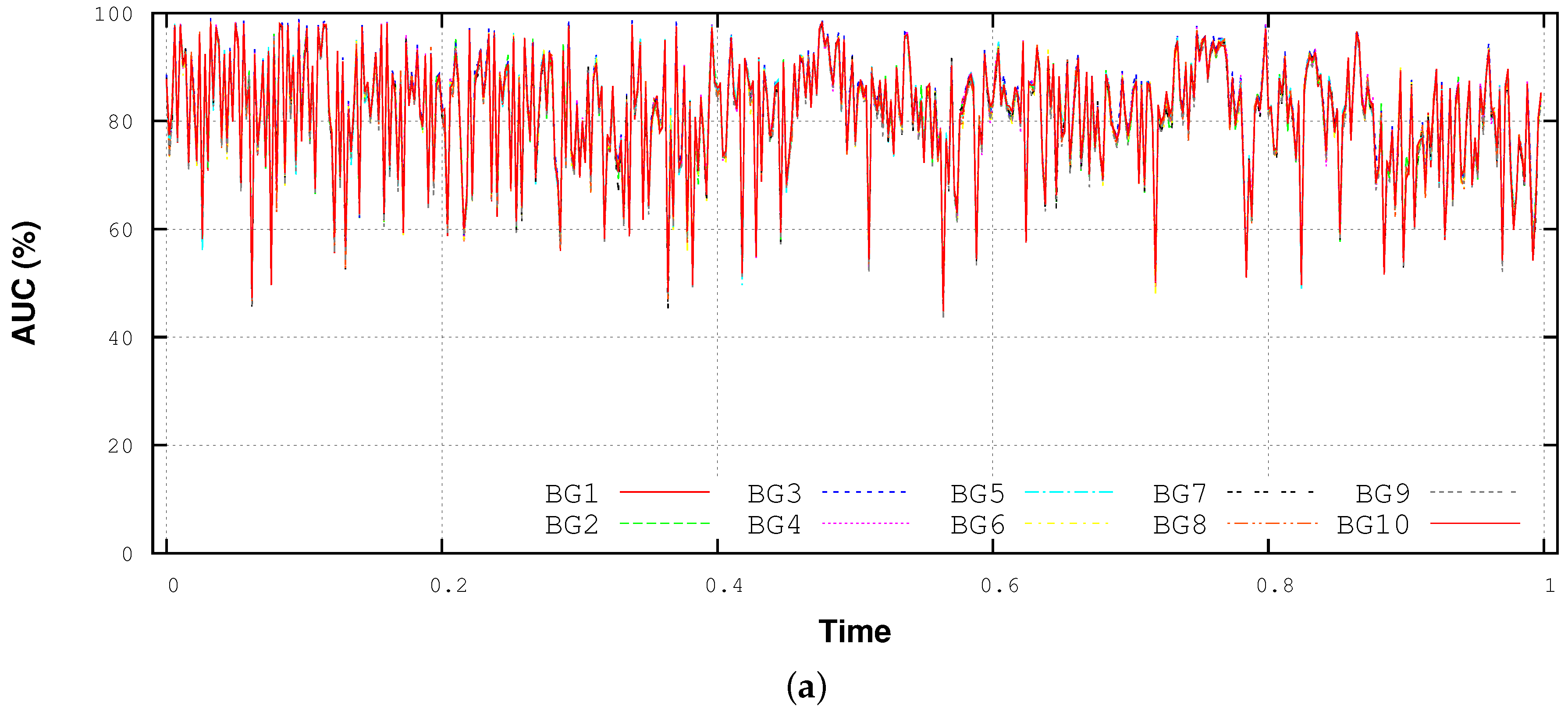
4.4. Performance Variability Analysis

In order to have a better insight into the system performance, in particular of the standard deviation shown in the results, a sensitivity analysis has been performed. As for the experiments discussed in Section 3, 10 leakages for 10 different background models have been considered, thus 100 evaluations for each condition. The tests have been performed for the higher resolution, 1 min, on both water and natural gas consumption of the AMPds, by using the best features’ combinations. Moreover, for each dataset and technique, the evaluations have been performed three times, and each time, two out of three leakage parameters have been kept constant, in order to perform the analysis of the leakage starting point, size and duration.

For the starting point sensitivity analysis, the leakage size is set to $\beta =0.375$, and the leakage duration is fixed to 450 samples. For the leakage size test, the starting point is kept to half of the set length, and the β has been varied from $0.25$ to $0.50$, as for the previous experiments. Finally, for the leakage duration sensitivity analysis, the leakage duration has been varied from 300 to 600 samples. The results, depicted in

Table 7. Performance of the variability tests.

Resource	Model	Leakage Starting Point		Leakage Size		Leakage Duration
		AUC (%)	SD	AUC (%)	SD	AUC (%)	SD
AMPds Gas	GMM	$89.09$	$9.48$	$87.88$	$3.39$	$88.57$	$1.41$
AMPds Gas	HMM	$89.10$	$9.67$	$87.49$	$3.64$	$88.20$	$1.44$
AMPds Gas	SVM	$54.75$	$20.07$	$69.20$	$0.16$	$70.75$	$1.76$
AMPds Water	GMM	$83.36$	$8.33$	$90.13$	$7.11$	$89.68$	$2.15$
AMPds Water	HMM	$89.90$	$9.58$	$94.46$	$4.88$	$94.84$	$2.85$
AMPds Water	SVM	$54.99$	$16.10$	$50.09$	$0.16$	$53.17$	$2.17$

, show that the bottleneck is due to the leakage position in the set, and a strong correlation between the leakage position and the achieved performance is revealed, as shown in Figure 9. In particular, for each background model, the AUCs evaluated for 500 leakage positions, uniformly distributed along the dataset length, are reported. All of the backgrounds present the same trend, and this confirms, for both GMM and HMM, that the standard deviation does not depend on the variability of the initial conditions in the training procedure, but it is entirely due to the leakage position in the dataset instead; thus, the backgrounds present the same envelope.

5. Conclusions

In this paper, a framework for automatic leakage detection in smart water and natural gas grids has been presented. The framework is made of an innovative set of features, actually missing in the related literature and specifically defined for the application scenarios under study, and a variation of the SFS approach proposed by the authors to select the best features. The framework core is represented by the novelty detector, implemented by means of three statistical algorithms, i.e., GMM, HMM and OC-SVM, which, to the authors’ knowledge, have never been used for the application scenarios under study.

Experiments have been focused on two distinct scenarios, i.e., the residential and building ones, for which the water and natural gas consumption values from the AMPds and DFID datasets have been respectively employed.

The achieved results confirmed the suitability of the proposed leakage detection approach for both case studies. In particular, the GMM and HMM models were revealed to be the best performing ones in terms of AUC, the quality index used for our assessments. The assumption of time-limited leakage models has proven the detection time to be reasonably short. Moreover, the usefulness of temporal information, especially for low sampling data rates, has been confirmed, as well.

Further investigations revealed a strong correlation between the leakage position and the achieved performance. To address this aspect of the problem, future works will investigate new features to lower the dependency of the system performance from the leakage parameters. Additionally, other types of anomalies, such metering system issues and faults, will be addressed in future works, along with temporal clustering.

References

1. WaterSense. Leak Facts. Available online: http://www3.epa.gov/watersense/pubs/fixleak.html (accessed on 30 October 2015).
2. Fagiani, M.; Squartini, S.; Gabrielli, L.; Spinsante, S.; Piazza, F. A Review of Datasets and Load Forecasting Techniques for Smart Natural Gas and Water Grids: Analysis and Experiments. Neurocomputing 2015, 170, 448–465. [Google Scholar] [CrossRef]
3. Spinsante, S.; Pizzichini, M.; Mencarelli, M.; Squartini, S.; Gambi, E. Evaluation of the Wireless M-Bus Standard for Future Smart Water Grids. In Proceedings of the Wireless Communications and Mobile Computing Conference, 9th International, Cagliari, Sardinia, Italy, 1–5 July 2013; pp. 1382–1387.
4. Spinsante, S.; Squartini, S.; Gabrielli, L.; Pizzichini, M.; Gambi, E.; Piazza, F. Wireless M-Bus sensor networks for smart water grids: Analysis and results. Int. J. Distrib. Sens. Netw. 2014, 10. [Google Scholar] [CrossRef]
5. Hao, W.S.; Garcia, R. Development of a Digital and Battery-Free Smart Flowmeter. Energies 2014, 7, 3695–3705. [Google Scholar] [CrossRef]
6. Quevedo, J.; Chen, H.; Cugueró, M.; Tino, P.; Puig, V.; García, D.; Sarrate, R.; Yao, X. Combining Learning in Model Space Fault Diagnosis with Data Validation/Reconstruction: Application to the Barcelona Water Network. Eng. Appl. Artif. Intell. 2014, 30, 18–29. [Google Scholar] [CrossRef]
7. Sadeghioon, A.M.; Metje, N.; Chapman, D.N.; Anthony, C.J. SmartPipes: Smart Wireless Sensor Networks for Leak Detection in Water Pipelines. J. Sens. Actuator Netw. 2014, 3, 64–78. [Google Scholar] [CrossRef]
8. Lobaccaro, G.; Carlucci, S.; Löfström, E. A Review of Systems and Technologies for Smart Homes and Smart Grids. Energies 2016, 9, 348. [Google Scholar] [CrossRef]
9. Hajebi, S.; Song, H.; Barrett, S.; Clarke, A.; Clarke, S. Towards a reference model for water smart grid. Int. J. Adv. Eng. Sci. Technol. 2013, 2, 310–317. [Google Scholar]
10. Siano, P.; Graditi, G.; Atrigna, M.; Piccolo, A. Designing and testing decision support and energy management systems for smart homes. J. Ambient Intell. Humanized Comput. 2013, 4, 651–661. [Google Scholar] [CrossRef]
11. Somma, M.D.; Yan, B.; Bianco, N.; Graditi, G.; Luh, P.; Mongibello, L.; Naso, V. Operation optimization of a distributed energy system considering energy costs and exergy efficiency. Energy Convers. Manag. 2015, 103, 739–751. [Google Scholar] [CrossRef]
12. Fagiani, M.; Squartini, S.; Bonfigli, R.; Piazza, F. Short-term Load Forecasting for Smart Water and Gas Grids: A Comparative Evaluation. In Proceedings of the 2015 IEEE 15th International Conference on Environment and Electrical Engineering (EEEIC), Rome, Italy, 10–13 June 2015; pp. 1198–1203.
13. Fagiani, M.; Squartini, S.; Severini, M.; Piazza, F. A Novelty Detection Approach to Identify the Occurrence of Leakage in Smart Gas and Water Grid. In Proceedings of the 2015 International Joint Conference on Neural Networks, Killarney, Ireland, 12–17 July 2015; pp. 1309–1316.
14. Markou, M.; Singh, S. Novelty Detection: A Review-Part 1: Statistical Approaches. Signal Process. 2003, 83, 2481–2497. [Google Scholar] [CrossRef]
15. Markou, M.; Singh, S. Novelty Detection: A Review-Part 2: Neural Network Based Approaches. Signal Process. 2003, 83, 2499–2521. [Google Scholar] [CrossRef]
16. Pimentel, M.A.; Clifton, D.A.; Clifton, L.; Tarassenko, L. A Review of Novelty Detection. Signal Process. 2014, 99, 215–249. [Google Scholar] [CrossRef]
17. Chis, T. Pipeline Leak Detection Techniques. CoRR, 2009; arXiv:0903.4283. [Google Scholar]
18. Murvay, P.S.; Silea, I. A Survey on Gas Leak Detection and Localization Techniques. J. Loss Prev. Process Ind. 2012, 25, 966–973. [Google Scholar] [CrossRef]
19. Mounce, S.R.; Mounce, R.B.; Boxall, J.B. Novelty Detection for Time Series Data Analysis in Water Distribution Systems using Support Vector Machines. J. Hydroinform. 2011, 13, 672–686. [Google Scholar] [CrossRef]
20. Nasir, M.; Mysorewala, M.; Cheded, L.; Siddiqui, B.; Sabih, M. Measurement Error Sensitivity Analysis for Detecting and Locating Leak in Pipeline using ANN and SVM. In Proceedings of the 2014 11th International Multi-Conference on Systems, Signals Devices (SSD), Castelldefels, Barcelona, Spain, 11–14 February 2014; pp. 1–4.
21. Rossman, L.A. The EPANET Water Quality Model; Coulbeck, B., Ed.; Research Studies Press Ltd.: Somerset, UK, 1993; Volume 2. [Google Scholar]
22. Gamboa-Medina, M.; Reis, L.R.; Guido, R.C. Feature Extraction in Pressure Signals for Leak Detection in Water Networks. Procedia Eng. 2014, 70, 688–697. [Google Scholar] [CrossRef]
23. Sanz, G.; Perez, R.; Escobet, A. Leakage Localization in Water Networks using Fuzzy Logic. In Proceedings of the 20th Mediterranean Conference on Control Automation (MED), Barcelona, Spain, 3–6 July 2012; pp. 646–651.
24. Alkasseh, J.; Adlan, M.; Abustan, I.; Aziz, H.; Hanif, A. Applying Minimum Night Flow to Estimate Water Loss Using Statistical Modeling: A Case Study in Kinta Valley, Malaysia. Water Resour. Manag. 2013, 27, 1439–1455. [Google Scholar] [CrossRef]
25. Oren, G.; Stroh, N.Y. Mathematical Model for Detection of Leakage in Domestic Water Supply Systems by Reading Consumption from an Analogue Water Meter. Int. J. Environ. Sci. Dev. 2013, 4, 386–389. [Google Scholar] [CrossRef]
26. Wan, J.; Yu, Y.; Wu, Y.; Feng, R.; Yu, N. Hierarchical Leak Detection and Localization Method in Natural Gas Pipeline Monitoring Sensor Networks. Sensors 2012, 12, 189–214. [Google Scholar] [CrossRef] [PubMed]
27. Vapnik, V.N. Statistical Learning Theory; Wiley-Interscience: New York, NY, USA, 1998. [Google Scholar]
28. Perner, P. Concepts for Novelty Detection and Handling Based on a Case-based Reasoning Process Scheme. Eng. Appl. Artif. Intell. 2009, 22, 86–91. [Google Scholar] [CrossRef]
29. Makonin, S.; Popowich, F.; Bartram, L.; Gill, B.; Bajic, I. AMPds: A Public Dataset for Load Disaggregation and Eco-Feedback Research. In Proceedings of the 2013 IEEE Electrical Power Energy Conference (EPEC), Halifax, NS, Canada, 21–23 August 2013; pp. 1–6.
30. Department for International Development. Live Data Page for Energy and Water Consumption. Available online: http://data.gov.uk/dataset/dfid-energy-and-water-consumption (accessed on 30 October 2015).
31. Principi, E.; Squartini, S.; Bonfigli, R.; Ferroni, G.; Piazza, F. An Integrated System for Voice Command Recognition and Emergency Detection Based on Audio Signals. Expert Syst. Appl. 2015, 42, 5668–5683. [Google Scholar] [CrossRef]
32. Kuncheva, L.I. Change Detection in Streaming Multivariate Data Using Likelihood Detectors. IEEE Trans. Knowl. Data Eng. 2013, 25, 1175–1180. [Google Scholar] [CrossRef]
33. Theodoridis, S.; Koutroumbas, K. Pattern Recognition, 4th ed.; Academic Press: Burlington, VT, USA, 2008. [Google Scholar]
34. Britton, T.C.; Stewart, R.A.; O’Halloran, K.R. Smart Metering: Enabler for Rapid and Effective Post Meter Leakage Identification and Water Loss Management. J. Clean. Prod. 2013, 54, 166–176. [Google Scholar] [CrossRef]
35. Bishop, C.M. Pattern Recognition and Machine Learning; Springer: Secaucus, NJ, USA, 2006. [Google Scholar]
36. Reynolds, D.A.; Quatieri, T.F.; Dunn, R.B. Speaker Verification Using Adapted Gaussian Mixture Models. Digit. Signal Process. 2000, 10, 19–41. [Google Scholar] [CrossRef]
37. Rabiner, L. A Tutorial on Hidden Markov Models and Selected Applications in Speech Recognition. Proc. IEEE 1989, 77, 257–286. [Google Scholar] [CrossRef]
38. Jurafsky, D.; Martin, J.H. Speech and Language Processing, 2nd ed.; Prentice-Hall, Inc.: Upper Saddle River, NJ, USA, 2009. [Google Scholar]
39. Baum, L. An inequality and associated Maximization Technique in Statistical Estimation for Probabilistic Functions of Markov Processes. Inequalities 1972, 3, 1–8. [Google Scholar]
40. Schölkopf, B.; Platt, J.C.; Shawe-Taylor, J.C.; Smola, A.J.; Williamson, R.C. Estimating the Support of a High-Dimensional Distribution. Neural Comput. 2001, 13, 1443–1471. [Google Scholar] [CrossRef] [PubMed]
41. Collobert, R.; Bengio, S.; Marithoz, J. Torch: A Modular Machine Learning Software Library. Available online: https://infoscience.epfl.ch/record/82802/files/rr02-46.pdf (accessed on 1 June 2015).
42. Chang, C.C.; Lin, C.J. LIBSVM: A Library for Support Vector Machines. ACM Trans. Intell. Syst. Technol. 2011, 2, 1–27. [Google Scholar] [CrossRef]
43. Ntalampiras, S.; Potamitis, I.; Fakotakis, N. Probabilistic Novelty Detection for Acoustic Surveillance Under Real-World Conditions. IEEE Trans. Multimed. 2011, 13, 713–719. [Google Scholar] [CrossRef]
44. Fawcett, T. An Introduction to ROC Analysis. Pattern Recogn. Lett. 2006, 27, 861–874. [Google Scholar] [CrossRef]
Figure 1. Framework stages: (a) normality model creation; (b) novelty detection.
Energies 09 00665 g001
Figure 2. Threshold example: the log-likelihood exceeds the threshold; the abnormal event detected (left circle); the log-likelihood does not exceed the threshold, normal event (right circle). The y-axis represents the log-likelihood value computed for each frame, while the x-axis represents the frame number.
Energies 09 00665 g002
Figure 3. Feature selection steps and corresponding features’ combination until the achievement of the best result for the AMPds datasets. In the x-axis are reported the corresponding best features’ combinations for both GMM and HMM.
Energies 09 00665 g003
Figure 4. Feature selection steps and corresponding features’ combination until the achievement of the best result for the DFID datasets. In the x-axis are reported the corresponding best features’ combinations for both GMM and HMM.
Energies 09 00665 g004
Figure 5. Comparison between the first steps of the standard Sequential Feature Selection (SFS) algorithm and its revised counterpart. For each step, the red text denotes the winner feature or the features’ combination. The red boxes denote the 3 different features sets generated starting from the 3 winner features of the previous step.
Energies 09 00665 g005
Figure 6. Example of flow data with induced leakage (a) and the corresponding set of extracted features (b). The dashed lines define the leakage start and end. For each frame, the reported features are the Ma, the En and the four components of the L w .
Energies 09 00665 g006
Figure 7. Examples of the ROC and AUC relations.
Energies 09 00665 g007
Figure 8. ROCs for the best achieved results with each background model. The red dotted line represents the overall mean curve. (a) AMPds gas; (b) AMPds water; (c) overall gas; (d) Whitehall House water.
Energies 09 00665 g008
Figure 9. AUCs achieved by GMM and HMM backgrounds in the starting point analysis. (a) GMM; (b) HMM.
Energies 09 00665 g009aEnergies 09 00665 g009b