Article

Optimization of the Heating System Use in Aged Public Buildings via Model Predictive Control

1
Automatic Control Group, Department of Thermal Engineering, University of the Basque Country (UPV/EHU), Bilbao 48013, Spain
2
Automatic Control Group, Department of Automatic Control and Systems Engineering, University of the Basque Country (UPV/EHU), Bilbao 48013, Spain
3
Enedi Research Group, Department of Thermal Engineering, University of the Basque Country (UPV/EHU), Bilbao 48013, Spain
*
Author to whom correspondence should be addressed.
Energies 2016, 9(4), 251; https://doi.org/10.3390/en9040251
Submission received: 16 January 2016 / Revised: 16 March 2016 / Accepted: 23 March 2016 / Published: 30 March 2016
(This article belongs to the Special Issue Energy Efficient Building Design 2016)

Abstract

:
This work presents the implementation of a Model Predictive Control (MPC) scheme used to study the improvement of the thermal quality in aged residential buildings without any rehabilitation. The controller manages the heating system of an experimentally characterized model of a residential dwelling in a social block built during the decade of the 1960s located in the neighborhood of Otxarkoaga (Bilbao, Spain), so as to obtain an optimal energy efficiency performance. Due to the characteristics of the construction in those days, this kind of buildings suffer problems related to the use of awkward building materials and inefficient heating systems. A comparison with traditionally used ON-OFF hysteresis control is presented in order to demonstrate the energetic improvement provided by the MPC scheme. Besides, the variation of different parameters of the MPC is also studied to determine its influence over the energy consumption and comfort conditions.

1. Introduction

The European Union should reduce its dependence on foreign sources of energy, whereby more than half of the consumed energy is imported [1,2]. European Union should also mitigate the global warming situation produced by the emission of greenhouse gases. Buildings, are known to be one of the most relevant sectors in energy consumption, together with transport and industry. The activity of this sector in Europe accounts for approximately 40% of the total energy consumption and 36% of CO2 emissions [3], which is one of the more important agents of the global warming [4]. In this context, great efforts are currently carried out in the building sector to develop energetic efficiency policies in order to comply with the objectives proposed by the European Energy Performance of Buildings Directive [5], which will be applicable to a new construction building. Despite this, there is an important existing building stock, which is far from meeting the objectives laid down in the directive due to its aging structures and outdated materials.
Adequate insulation and building materials or enhanced windows can be considered passive improvements of new buildings or in the rehabilitation of the old ones. The development of a control to improve the energy efficiency in the use of the climate control systems within the required comfort parameters can be considered an active improvement. The Model Predictive Control (MPC) supposes an excellent control option [6,7,8,9,10,11] since it does not only consider the information related to the system at an operation instant, but it also takes into account the predicted future information related to the weather or building use so as to obtain an optimal control action.
Given the model of the thermal behavior of an aged building without any rehabilitation, which has been obtained in an experimental study, a simulation of the impact of an MPC in its heating system has been evaluated against the classical ON-OFF thermostatic control. The results aim to give an approximation of the possible energy savings that the use of this control may represent in this kind of aged buildings, which is even more relevant considering its large stock and that most of the bibliography deals with new design buildings with improved materials and climate systems.
This novel MPC implementation has been successfully applied considering a reduced model that has been obtained experimentally. However, the reader may be interested in more complex MPC models such as those given in [12,13] where the reference tracking for the heating system is ensured or [14] where MPC is applied over a low energy building with a long prediction horizon of two days. Other kind of advanced control policies can be deployed in building climate systems as those presented in [15] where the thermostat control is improved by a learning policy [16,17], where neuro-fuzzy control is used as the control of an indoor temperature: The Artificial Neural Network (ANN) provides a forecasted indoor temperature to be used by a dynamic Fuzzy Logic Control (FLC), which in this case is a clear enhancement over other multi-criteria control strategies as the Ruled Based Controls (RBC). Finally [18] presents another predictive control based on neuro-fuzzy controls.
The main aim of this paper is to show the benefits that the use of an MPC can suppose in the control of buildings designed with poor construction material and systems. Using the model of a dwelling of these characteristics that has been developed in an experimental way, the predictive characteristics of the MPC are used to simulate the behavior of the dwelling and evaluate the energy saves in the heating system.

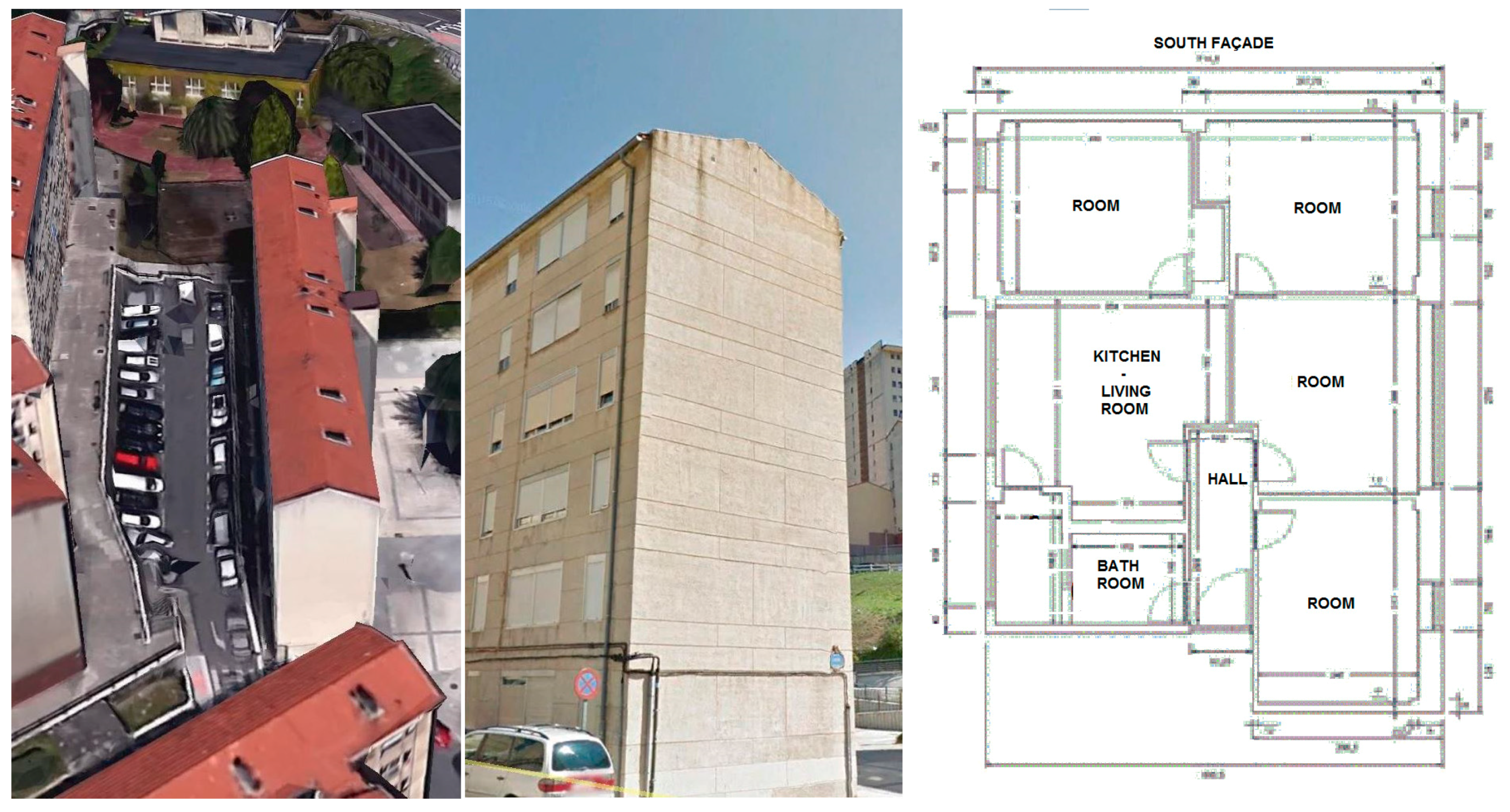
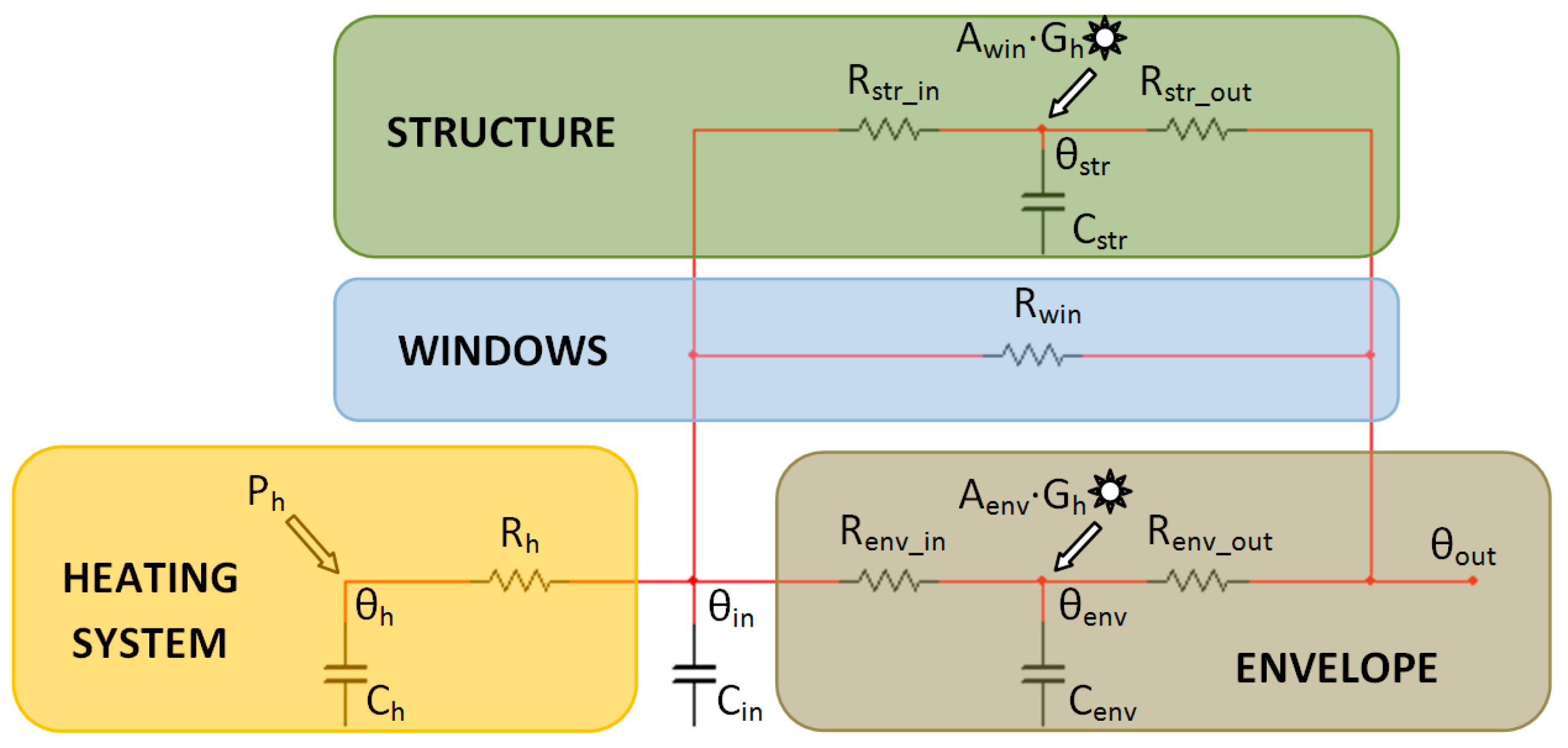
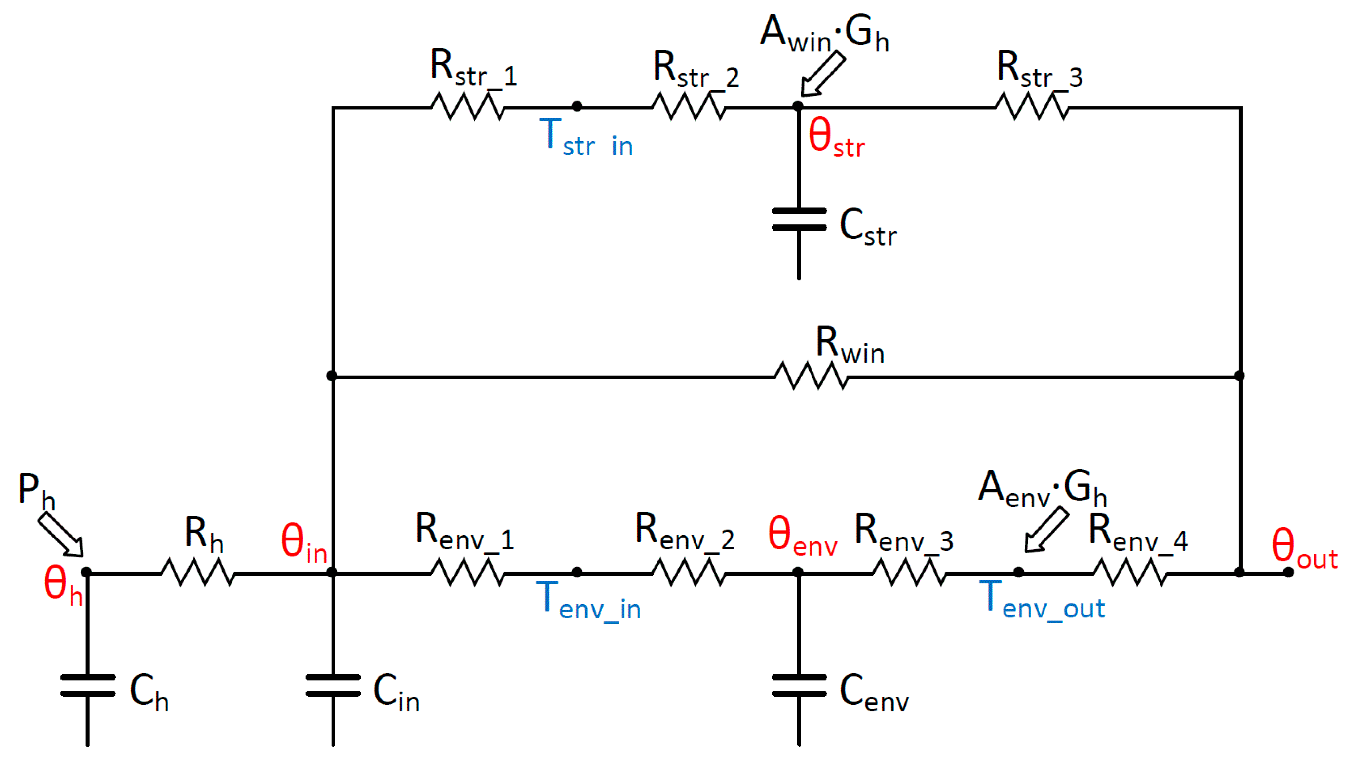
2. System Description

The public organization Bilbao Municipal Housing has defined different building typologies in its housing stock in order to study their energetic behaviour and to take adequate actions to ensure a better thermal response and to minimize the energy consumption. The study was mainly focused on the improvement of the construction materials, adding insulating materials or replacing the low thermal resistance windows with improved new ones. This paper studies the improvement associated with the energy consumption using MPC control method on the aforementioned dwelling.
The dwelling selected for the study is part of a social housing block, with east-west orientation and located in the neighbourhood of Otxarkoaga, in Bilbao (43°15.5′N, 2°54′W, Figure 1), which is a representative building of the social housing buildings built during the industrial city growth of the sixties. It has a concrete structure, airbrick envelope with air chamber but with no other kind of insulation either in the envelope or in the windows. There is an individual heating system for the dwelling with no cooling or ventilation system. With 50 m2 of floor area it is a typical social building of the late fifties, sixties and early seventies, not only in this region but also in most of the industrial regions around Europe. The sheer amount of buildings of these characteristics is a reason in of itself for the thermal study and the simulation of the MPC implementation.
The study performed to evaluate and to model the thermal behaviour of the dwelling [19] was developed during the winter season in 2012. In order to obtain a thermal model for the building, the behaviour of one dwelling in the building was measured over time. With the dwelling empty, the air temperatures of the different rooms were obtained over time as well as the wall surfaces temperatures and the heat flux through the façade to evaluate the losses through it. Weather conditions, temperature and solar irradiation were measured too. Measured data were collected every minute and an average value was stored for each parameter with a time step of 10 min.
In order to improve the analysis of the dynamic response of the dwelling, some heating power pulses were developed in a pseudorandom way by the heating system of the dwelling. The characterization of these Randomly Ordered Logarithmically distributed Binary Sequence or ROLBS [20], is used to decouple the internal and external influences that appear in the system and get adequate information for the recognition of the parameters in the process of creating a grey box RC-model that can be implemented in the MPC. Other pulse patterns such as Pseudo-Random Binary Signal or PRBS [21] may also be used in this kind of parameter recognition proceses as proposed in [22].
Statistical software used to determine the values of the thermal resistances and capacitances that characterize the dynamical thermal behaviour of the dwelling were obtained using the Continuous Time Stochastic Modelling package for R (CTSM-R). The package has been programmed at the Technical University of Denmark (DTU) [23] and adds some stochastic terms to the deterministic system in the parameter recognition process, as it will be seen in the next point. Other software programs that can be used for parameter recognition are LOgical R-Determination (LORD) [24] or GreyBox toolbox [25].
During the data acquisition, the maximum outdoor temperature was 20 °C and the minimum −0.3 °C and in order to achieve the comfort specifications for the inhabitants, the values of the indoor temperature inside of the house are set to 20 °C by day and 17 °C at night, which are maintained by a 5 kW heating boiler.
Building simulation software like TRNSYS [26] or EnergyPlus [27] can be used to represent the dynamic behaviour of a building using more detailed models, which apply the information associated with the constructions characteristics of the building such as thermal specifications of the utilized materials [28,29,30], climate control systems [31] and volume distribution. These programs are not adequate to develop a MPC-like control due to the lack of a mathematical model that can be developed over time, so they are usually used for simulation and certification. It must be mentioned that the IDEAS [32] library for modelica [33], allows the development of component based models to simulate systems associated to buildings but also to get a mathematical linear time invariant (LTI) model of the building in state space, so as to enable the application of MPC-like controls. In this case, and due to the large number of states that usually define the buildings when the model is developed from constructive parameters, its dimension should be reduced using known space reduction techniques like [34,35] or directly using resources such as the ones provided in MATLAB-like software, which will drop the computational requirements.
The parameters of the model that will be presented in the next section have been obtained from measuring from the real building; the model of the building will be reduced to a 4th order system, getting the average value of all the room temperatures for the internal temperature, as well as for the structure, envelope and heating system.3. RC-Model
To define the model, Figure 2, over which the MPC will be implemented, the dwelling is defined as a unique space that represents its entire volume in which no local variations of the temperature are considered. The different elements of the dwelling are represented in a RC-model by heat sources, thermal resistances and capacitances, which model the heating system apart from the structural elements and opaque and semitransparent-windows-envelope. The values of the outdoor temperature [35] and the solar radiation over the opaque and semitransparent envelope provide the external conditions that determine the evolution of the indoor temperature.
The model is defined as a state space system that will characterize the dynamics of the dwelling and where the different states in a continuous mode for the state θi are defined by:
C i θ ˙ i =   j θ j θ i R i j + k P i k
where Ci is the thermal capacitance associated to the θi state, Rij the thermal resistance between the states i and j and Pik are the heating fluxes applied over the θi state.
The temperatures of the elements of the building –indoor, structure, envelope and heating system– are grouped together in the state vector: θ = (θin θstr θenv θh)T which defines the situation of the system in each moment. Equation (2) represents the dynamic evolution of the system in state space form. Thus, in the case under study, besides the state vector, θ, the power supplied to the dwelling is defined by u = (Ph), what is calculated by the control. The influence of other factors such as outdoor temperature, θout, or solar radiation, Gs, that is designed by the measured or predicted disturbances is defined by v = (θout Awin·Gh Aenv·Gh)T, being Gh·Awin and Gh·Aenv the solar influence over the windows and envelope with Awin and Aenv their respective effective area. The output of the system, indoor temperature, is denoted y = (θin):
θ ˙ = A c · θ + B c u · u   + B c v v y = C · θ + D u · u   + D v v
where Ac, Bcu, Bcv, C, Du and Dv are the matrices associated with the continuous system. The complete matrix system is developed in [36].
In order to use the model with the measured data of the dwelling, the system has to be discretized. The large time constant associated with buildings like systems denotes that its dynamics are slow enough to discretize the system with the used time step, Ts, of ten minutes or even greater. In the present case, the discretization was performed using zero order hold (zoh) method and the discrete system is defined by:
θ k + 1 = A · θ k + B u · u k   + B v v k y k = C · θ k + D u · u k   + D v v k
where the k subscript indicates the evaluated moment and the A, Bu and Bv are the discrete matrices obtained using the zoh discretization with Ts sample time.
As described in the previous section, the parameters that define the RC-model, capacitances and resistances, were obtained by applying the CTSM-R package over the values obtained in the experimental measurements. For that, the dwelling was modelled so the measurements obtained are the ones represented in the model of the Figure 3. In that way, the thermal behaviour of the envelope (env) is evaluated measuring the temperatures of its internal and external surface in different points and then calculating its average; it is represented by a two resistances, one capacitance model. The structure and the internal walls of the dwelling (str) are considered in a similar manner. The interior temperature of the air is the average of the different rooms, the difference of temperature between different rooms at the moment of the data acquisition was never higher than one degree Celsius. No capacitance is associated to the windows (win) that are considered just like a resistance.
Rh is the thermal resistance between the heating system and the indoor air, Renv_2 and Renv_3 are the resistances of the envelope, and Renv_1 and Renv_4 are the ones associated to the thermal conductivity between the surface and the air. Similar notation is given for the structure: Rstr_2 and Rstr_3 with Rstr_1 being the resistance between the inner surface and the air. Rwin is the thermal resistance associated to the window. Ch, Cin, Cenv and Cstr are the capacitances associated to the respective elements. All these parameter values are estimated by the software given the experimental values for the temperatures θh, θin, θout, Tenv_in, Tenv_out and Tstr_in, the solar radiation through the windows Awin·Gh and over the envelope Aenv·Gh as well as the power of the heating system, Ph.
The package uses stochastic terms to improve the accuracy of the parameters obtained, these terms that give an idea about the possible disturbances in the measurement of the parameter are considered in the state space system that is defined by:
θ ˙ = A · θ + B · u   + σ d ω y = C · θ + D · u +   σ e
where θ is the state vector that defines the temperatures, A, B, C, D are the matrices that define the system, the u vector is defined in this case by the measured values that are used to determine the parameters of the system: Outside temperature, Tout, solar irradiance, Gh, temperature of the surface of the envelope or structure, Tenv_in, Tenv_out, Tstr_in, temperature of the heating system, Th, power issued by the heating system, Ph. The value ω represents a standard Weiner process and e a white noise process.
The necessary information about the mathematical model used by CTSM-R can be found in [37,38,39], were the statistical instruments to acquire and check the values of the parameters that describe the system are explained. The values obtained in the parameterization process can be found in [19] and have been added to the article in table of the Appendix A. Once the values are determined, the system can be rewritten to take the shape of the one described in Equation (2) and in Figure 2.
Due to the simplicity of the dwelling structure and of the installed heating system, the model may be described by a linear system. In the study of more complex buildings and climate control systems [36,40,41,42], nonlinearities may arise due to the relations that can appear between the control variables (u) and some of the states (θ) or measured or predicted disturbances (v), such as the ones that appear between the outdoor temperature and an air heating system or between a blind system and the solar radiation. In such cases, the system evolution is defined by:
θ k + 1 = A θ k + B u u k + B v v k + i = 1 n u ( B u v , i v k + B u x , i θ k ) u k , i
where Buv, Bvx are the set of matrices associated with the nonlinear relations.
Besides the linearization around the operation point, different methodologies are proposed to treat the problems associated with the nonlinearities [42]. The work developed in [43] can be considered especially interesting due to its development level and implementation characteristics.

Comfort Conditions for Comfort Requirements

In order to implement a control for the climate system of a building, office or dwelling, it is necessary to determine the parameters to be controlled and the range in which the control has to maintain them. In particular, the comfort conditions have to be set. At this moment, there is not a European norm for these conditions and therefore local regulations will be considered. The Technical Code for Edification (DB-HE) [44] determines the local normative that defines these comfort parameters in Bilbao for the residential buildings. In the case of the dwelling under study, due to its characteristics, the unique parameter to be controlled is the indoor temperature. The temperature is defined in the aforementioned Technical Code to be 20 °C (from 08:00 a.m. to 23:00 p.m. hours) by day and a minimum value of 17 °C by night (23:00 p.m. to 08:00 a.m.). A comfort band of 2 °C by day and of 1 °C by night is defined over these reference values. The use of this band allows some more flexible control strategies that will mean a decrement in the power consumption, as will be seen latter. The variation of the reference temperature from day to night is determined by the normal use of the residential building.
With the aim of reducing the energy consumption, a new trend called adaptive comfort is now developed [30,45] and it is already introduced in the norms ASHRAE 55 [46], where is defined as an optional way to determine the comfort, and ISO 7730 [47], where is defined as informative. The comfort of the building it is not only determined by the indoor temperature but also by parameters such as the operative temperature, the humidity of the air and its speed, the clothes the users wear and the outside temperature. The operative temperature is a mix between the indoor air temperature and the radiant one, to evaluate the heat loses by convection and radiation. Predicted Mean Vote (PMV) and Percentage of People Dissatisfied (PPD) are proposed indices to determine the thermal comfort quality in a building. Due to the typology of the dwelling under study where the only actuator available for control is the heating system, the deviation of the indoor temperature from the comfort band has been computed in hours·K, which is another usual unit [30]. It is necessary to note that the reference for comfort in the aforementioned Technical Code is only the indoor temperature.

3. Model Predictive Control Scheme

The main objective of this paper is to study the effect that the use of an advanced control such as an MPC has on the energy consumption of the heating system of a building of the described typology.
The MPC is a kind of advanced control that gets the optimal control action for a modelling system over some weighted conditions and restrictions, taking into account the evolution of the system over a defined period of time denoted predicted horizon, Np. In the case under study, the energy consumption of the heating system of a dwelling, the control has to minimize the use of the energy while the indoor temperature fulfils some comfort conditions: to be inside of the comfort band and try to fit a reference temperature.
Having an RC-model for the dwelling, such as the one of the Equation (3), it is possible to control the system over the time if future factors like solar radiation, outside temperature, usage patterns or applied heating power are known or can be predicted. Restrictions over the different parameters of the system can also be defined. MPC fully exploits this knowledge to get an optimal control response, heating power, that makes the indoor temperature of the dwelling be inside a comfort band by minimizing a cost function over the desired period. A full control pattern is obtained for the desired period after the minimization is done, which should be the best one under the proposed weight relations and restrictions. The first control action of this pattern is implemented by the control and, in order to get an adequate response, a new control action is calculated for the new time step. This knowledge of the future conditions for the system allows anticipating the control actions before the system arrive to those conditions. As an example the adaptation of the heating system before weather changes, the “in advanced” action of the control to arrive to a reference change “on time” ... can be mentioned.
In the case under study, the control action, u, is evaluated every ten minutes by minimizing the cost function, J0), which is usually defined as a quadratic function for the control action and the output. In order to trim the actions of the different parameter in the functions, these are weighted by some symmetric matrices (Q, R) that will determine the control action for instant k:
J ( θ 0 ) = min u 0 u N 1 k = 0 N p 1 ( ( ω y ) k T Q ( ω y ) k + u k T R u k )
where θ0 is the state vector at the current moment, ω is the reference value for the controlled variable, y is the output vector of Equation 3 where θin -indoor temperature-, is defined in, and (ω − y)k is the deviation between the reference temperature, Tin that is one of the components of the ω vector, and the indoor temperature, θin, at k instant. uk is the vector that defines the control action and Np the limit of the prediction horizon.
The definition of some constraints for the system will restrict the minimization of the cost function J0). These are:
0 < u < MaxPower
T min , k < θ i n , k < T max , k
The first one determines the range of power of the heating system. The second one determines the comfort band between Tmin and Tmax defined for the indoor temperature at the k moment, these temperature constraints can be changed over time but cannot be violated.
In order to define the constraints of the comfort band in a more realistic way and to avoid some possible problems in the resolution of the minimization, it is possible to soften the second constriction allowing a small transient violation of the limit by penalizing the violation itself. In this case, the constriction should take the form:
T min , k ε i < θ i n , k < T max , k + ε k
where ε is the parameter that will allow the comfort band to be overridden but will be heavily weighted in the J0) cost function that will be redefined as:
J ( θ 0 ) = min u 0 u N 1 k = 0 N p 1 ( ( ω y ) k T Q ( ω y ) k + u k T R u k + ε k T S ε k )
where S is the weight of ε, that should be much bigger than the other weights.
The minimization of the J0) function is the kernel of the MPCs. This is the reason why the choice of a suitable solver is critical. To tackling a complex problem, with a large number of states and restrictions that can vary over the time, the use of solvers like CPLEX [48] with an interpreter like YALMIP [49] could be a good option to accelerate the resolution process, to render it more stable and to get an enhanced control over the parameters and them variation. With this kind of solvers it is possible to minimize the integer-programming problems that sometimes appear solving minimizations due to the restrictions involved in the system.
Another parameter may be defined for the MPC: the control horizon, Nc, which will indicate the number of actions of the control variables to be optimized in a k control interval and fulfil the 1 < Nc < Np condition. If its value is too small, the result for the control action will not be satisfactory due to the few control actions computed each step. Too large value of Nc can delay the solution of the minimization without bringing any significant contribution into the control action.
An unconstrained MPC can be solved in the following way: for each iteration, the values of the state variables, control values and predicted influences:
θ = ( θ 0 θ 1 θ N p ) T   u = ( u 0   u 1   u N c ) T   v = ( v 0   v 1   v N p ) T
are computed according to Equation (3). θi, ui and vi are the state vector, control actuation and the values of predicted variables for i-th steep. Nc, control horizon, is the number of steps in which the controller action will be computed.
The set of state vectors, θ, is defined by:
θ = F θ 0 + Φ u u + Φ v v
where:
F = [ I A A 2 A N p ] ,   Φ u = [ 0 0 0 B u 0 0 A B u B u 0 A N p 1 B u A N p 2 B u A N p N c B u ] , Φ v = [ 0 0 0 0 B v 0 0 0 AB v B v 0 0 A N p 1 B v A N p 2 B v B v 0 ] .
The number of row and columns of the matrices is determined block-wise by Np and Nc, being F, Φu and Φv designed to create θ, so as to satisfy the cost function. The action of the control horizon can be clearly observed in the Φu matrix:
J ( θ 0 ) = min ( ( ω θ ) T 𝓠 ( ω θ ) + u T 𝓡 u )
where ω = (ω0 ω1 … ωNp)T is the vector that provides the temperature references over the time and the weigh matrices are:
𝓠 = [ Q 0 0 Q ] 𝓡 = [ R 0 0 R ] .
The minimization of u in the equation set specified in Equation (13) gives the control action set for the heating system at each given time step.

4. Experimental Studies

A study is performed to evaluate the plausible improvement in the energetic efficiency associated with the implementation of an MPC over the RC-model of a representative low thermal quality dwelling.
In the first part of the study, the implementation of the MPC over the model of the dwelling will be studied. The second part will compare the results obtained with the MPC with the ones obtained using an ON-OFF hysteresis control that is the usual thermal regulation system in dwellings. The last part of the work will study the way the different parameters of the MPC have influence on the accuracy of the control and in the energy consumption.

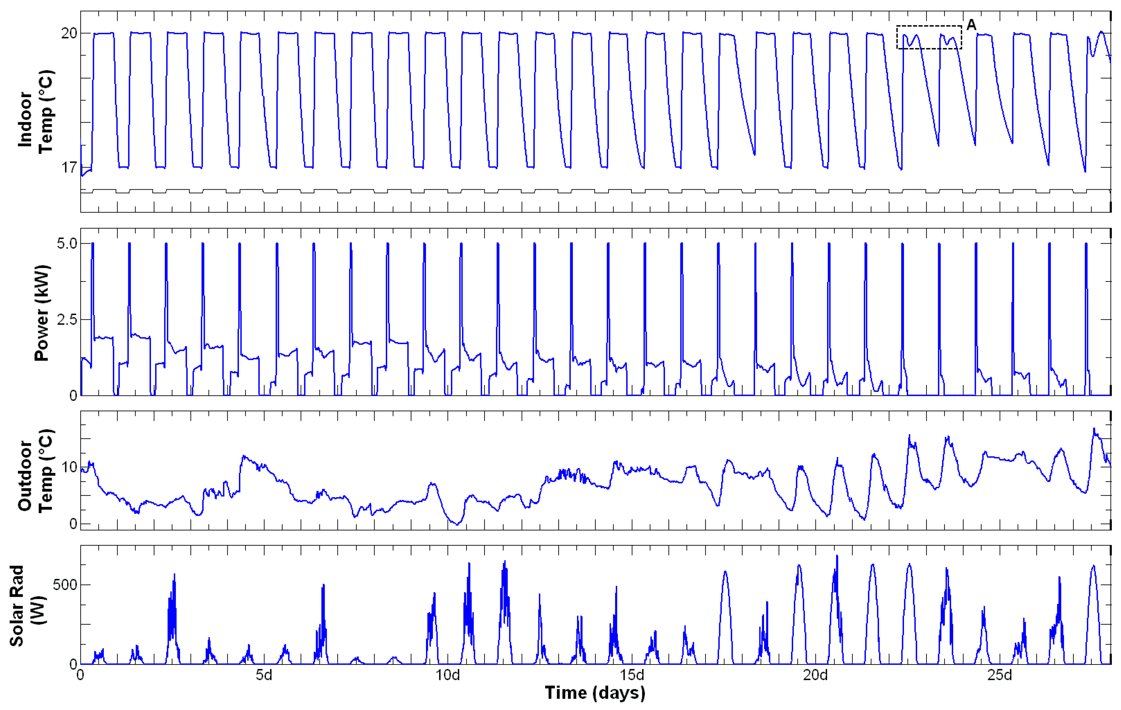
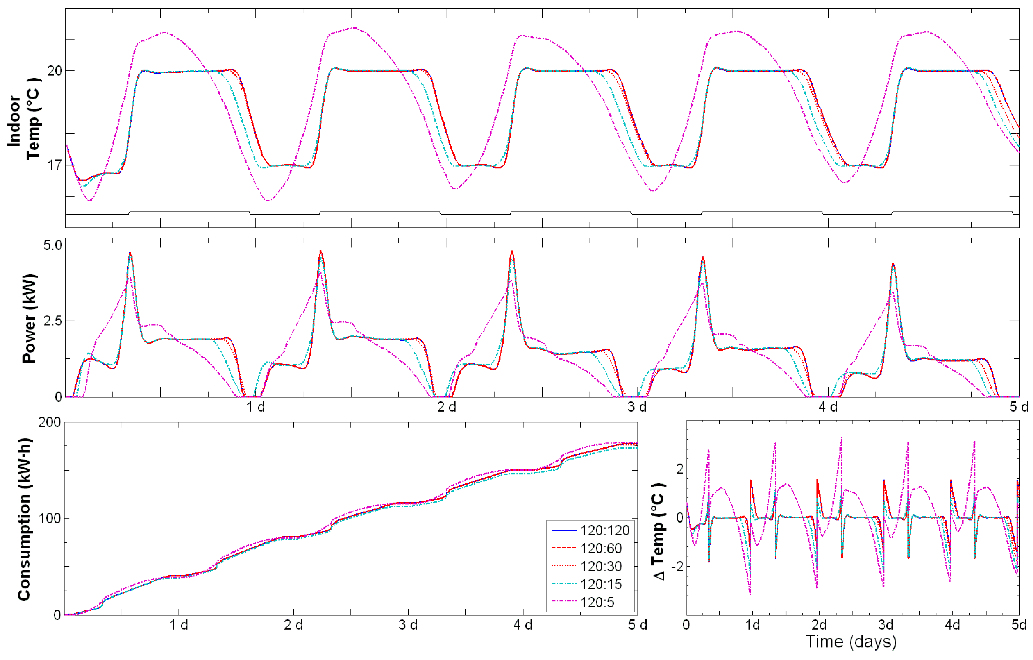
4.1. MPC Implementation

In Figure 4 the effect of the implementation of the MPC over the model of the dwelling can be observed. Environmental parameters appear in the Outdoor Temperature and Solar Radiation diagrams. The global heating power for the dwelling is 5 kW, it is necessary to indicate that in the experimental measurements, the maximum temperature difference between the rooms has never arrived at 1 °C, so a good heat distribution can be considered. After some initial simulations, it has been observed that a moderate prediction horizon, from 8 to 20 h, can be selected for the control due to the small capacitance and thermal resistance of the structure and envelope that defines a low thermal inertia building.
In order to observe the accuracy of the control, the cost function J(θ) that appears in Equation (9) has been designed so that the deviation of the indoor temperature with respect to the referenced one: ω − y is penalised heavier than the energy consumption, u. This means that the control fits the indoor temperature to the reference in a mostly perfect way during the day. The lack of a cooling system supposes that the night reference has to be reached by natural cooling and it will not be possible to reach the control reference as quick as it is predicted to be required by the reference change. This aspect does not really matter since the night comfort has not been exceeded by its low limit, it is more, if the reference condition is relaxed or even deleted at night, the control will minimize the consumed energy maintaining the temperature inside the comfort band for a non-critical period of the day.
In A section of Figure 4, the predicted effect of the control can be observed, due to the predicted influence of solar radiation and outside temperature, the indoor temperature should exceed the reference, to avoid this, the heat supply from the heat system is stopped and solar radiation becomes the source of the heat for the system.
Figure 5 displays a zoom of three days of Figure 4 that represents indoor temperature evolution, the power consumption pattern and the difference of the indoor temperature in respect to the temperature set point. The prediction effect of the MPC in respect to the reference signal and meteorological factors is again clearly represented. The control action begins before the reference change, which prepares the system to reach the day reference on time. When the temperature is reaching the day-reference the control action decreases and the temperature value is attained without the overshot that typically appears in other kinds of controls. Although this is not too important for the comfort, it means a better control pattern and lower energy consumption. In a non-predictive control, the control action should begin at the reference change point, which supposes that the dwelling should not be hot enough at the beginning of the morning. In order to observe the response of the system, two power systems are studied: 2.5 kW and 5 kW. Both systems fulfil the requested comfort conditions, but although greater power means a faster response, it also supposes means a higher energy consumption that can represent 5%. It may be mentioned that the 2.5 kW system power consumption apparently goes close to the 5 kW one right before 08:00 a.m., when the reference change will be produced; this is due to the MPC predictive behaviour, when the system maximum power used in anticipation so as to achieve the required temperature on time. The same behaviour is observed in the 5 kW system in a shorter time period. Predictive performance is also observed before 23:00 p.m., when the power systems switch off in order to save energy maintaining the dwelling inside the comfort band.

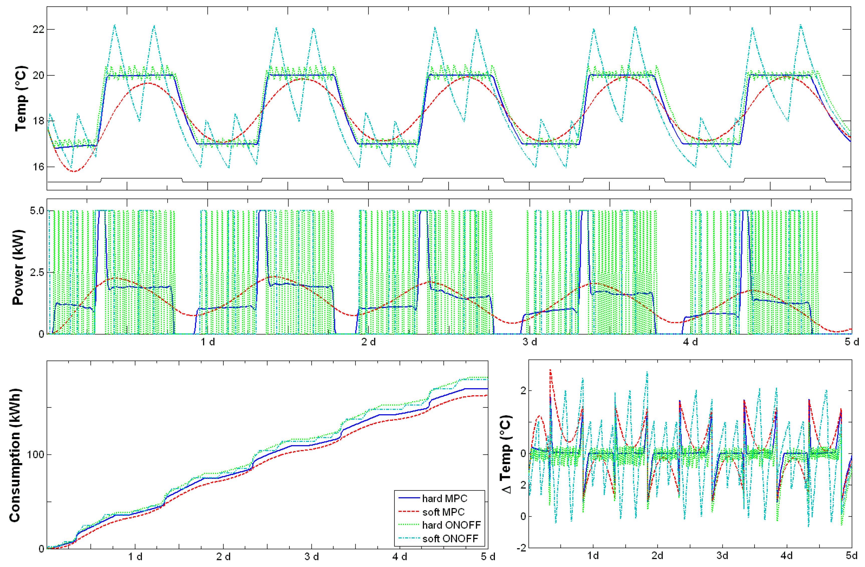
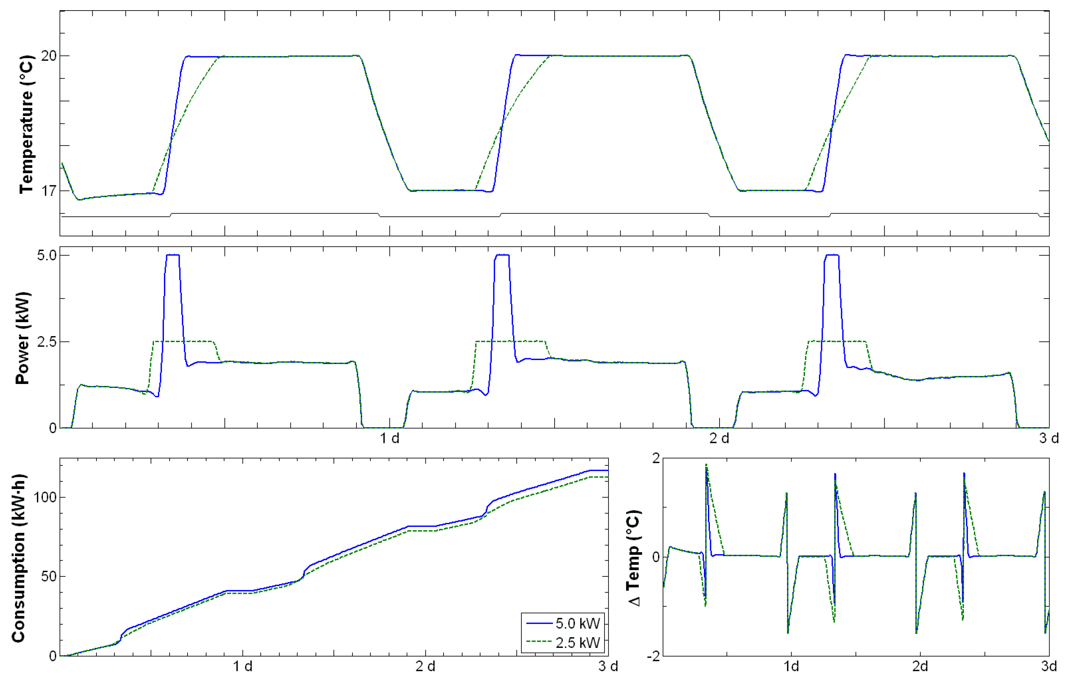
4.2. MPC vs. Histeresis Control

In Figure 6, a comparison between ON-OFF hysteresis control and MPC has been performed. The most common automatic heating system is a thermostat working over a hysteresis band that switches the heating power on or off when thermally defined limits are exceeded. Two hysteresis controls will be compared with the MPC, the first one, which will be called hys_SOFT, determines its hysteresis band over the limits of the comfort band, the second one, called hys_HARD, will determine its band over an extremely small deviation from the reference. This last control is not realistic, but is considered as a consumption reference. Values appear in Table 1. To adequate the temperature of the dwelling by morning, the system moves the night-day reference forward, so it is possible for the system to get the desired reference temperature by the morning. Something similar happens at the day-night reference change. Some other controls with hysteresis bands have been simulated obtaining similar energy consumptions.
Two MPCs are defined to be compared with the hysteresis controls, both have the same parameter but the relationship between the weights of the temperatures differs from the reference and the used power. The first one, called MPC_HARD, will try to follow the reference value leaving the energy consumption as a secondary objective. The second one, MPC_SOFT, knows which the temperature reference is, but the energy saving will be a main objective, maintaining the system inside the comfort band defined in the same way that the upper and lower limits of the hys_SOFT control. The values of the weights assigned to the MPC appear in Table 2.
Figure 6 gives the results of the simulation over a five day period. Some patterns appear when the whole month is studied:
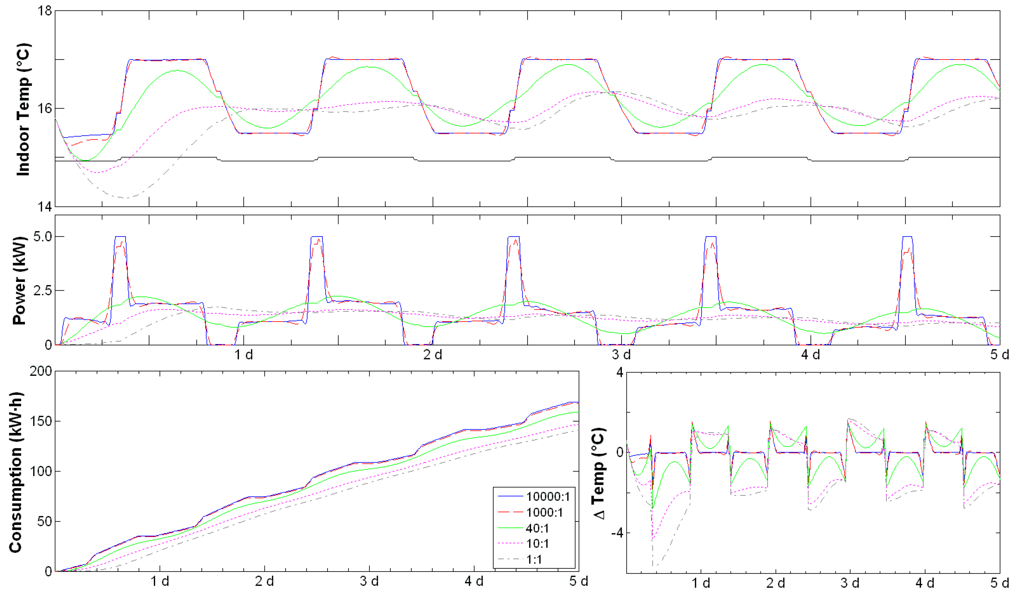
  • For the same kind of control, MPC or hysteresis, the energy consumption is greater when the control tries to follow the reference in a hard way. The MPC_SOFT gets an improvement of 7% in the energy consumption respect to the MPC_HARD as can be seen in Table 3.
  • A clear improvement appears when MPC and hysteresis controls are compared; when HARD models are compared the obtained improvement for the MPC is about 9.1%, when SOFT models are compared the improvement rises to 14.9%.
Finally, it can be said that the obtained results in the evaluated period for energy savings using MPC are in agreement with those obtained in [14,50], where energy savings of 10% are obtained for office buildings that use RBC.

4.3. Parameters of the MPC

In this section, some of the relations of the most important parameters of the MPC will be analyzed. First, the relation between the weights of the cost function will be studied and then how the relation between the prediction and control horizon affects the control action will be examined.
Before continuing with the study, it must be accentuate that one important characteristic for a successful MPC is the relationship among the weights assigned to the different parameters that appears in the cost function. These weights will be used to implement different control policies that, together with the restrictions applied to the system can prioritize different actions in order to maintain a constant temperature, optimize the system use to minimize the power usage [32], gas emissions or monetary cost, as well as discriminate the system between different heating systems or different time slots.
In the case under study, the main parameters of the cost function are the accuracy of the temperature to the setpoint and the energy consumption. As it has been seen, variations in this relation can induce an important deviation respect to the reference temperature, even when it is maintained inside the comfort band, as well as significant savings. Simulations are performed with the relations given in Table 4, were the relation between the weights, the energy consumption and the hours of thermal discomfort that appear in the dwelling during the month of February are presented. In Figure 7 the results of using five different controls over a five day period may be observed.
Table 4 indicates the energy consumption of the system for the control with different weights. As it can be observed, the values obtained are different than the ones obtained in Table 3. Table 3 uses predictive horizon of 100 steps (~16.7 h) and control horizon of 40 steps (~6.7 h), meanwhile the predictive and control horizons of Table 4 are 120 and 60 steps (20 and 10 h). A small variation between the two tables—consumptions and savings—can be observed due to the different values of the horizons. The chosen horizons are long enough to obtain a good control action with small differences between their consumptions. Considering the energy savings between the energy saving policy, 40:1 weight relation, and the reference tracking policy, 1000:1, it can be seen how the energy savings are almost the same: 6.5% vs. 7% for Table 3 and Table 4.
In Figure 7, it is possible to observe how for the 10,000:1 and 1000:1 cases, the control fits the desired reference perfectly, with no representative difference. When the weight associated with the energy consumption increases, 40:1, the control does not fully fit the indoor temperature to the reference, but maintains it in the comfort band. The temperature exhibits some variation but no thermal discomfort appears. For the next two models, 10:1, 1:1, the control does not maintain the temperature inside the comfort band so, even when it is possible to get energy savings, this is at the loss of thermal comfort. The hours of thermal discomfort associated with these controls in the whole month of February have also been evaluated in Table 4. Thermal discomfort hour is defined as the time the room temperature is out of the thermal comfort boundaries per the degrees it is out. In order to understand the values of the weight it is necessary to remember that the deviation from the reference temperature will be as much as a few degrees, while the value of the control action will change between 0 and 5000 W.
In Figure 8, the consequence of the variation of the control horizon for a known prediction horizon can be observed. As it has been mentioned in the previous point, while large values of the control horizon do not improve the control action enough to compensate the required computational effort, small control horizon values will provide an undesired control action. In this sense, control horizon values between the prediction horizon and a quarter of its value provide an accurate response of the system, while smaller control horizons will put the system out of the comfort band.

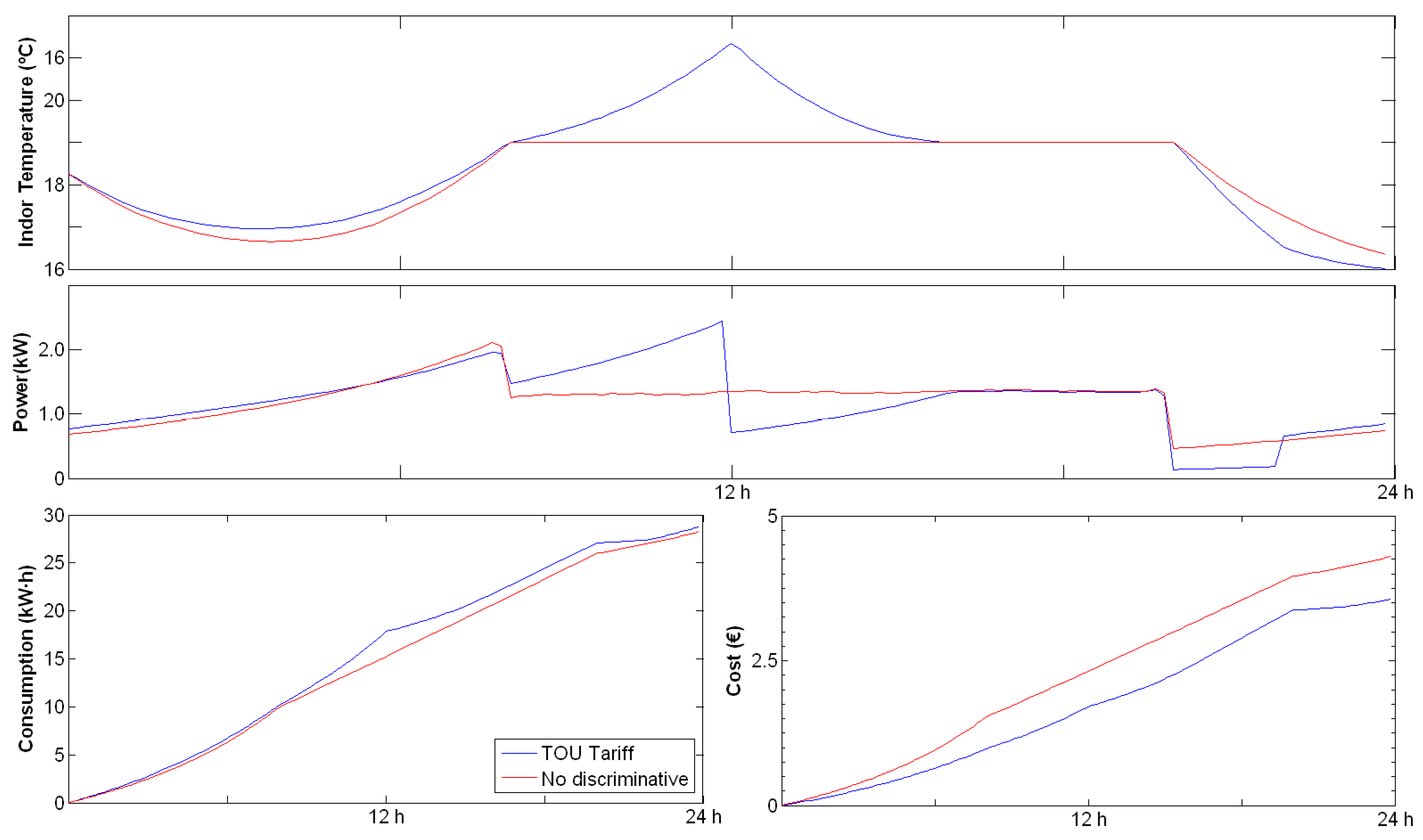
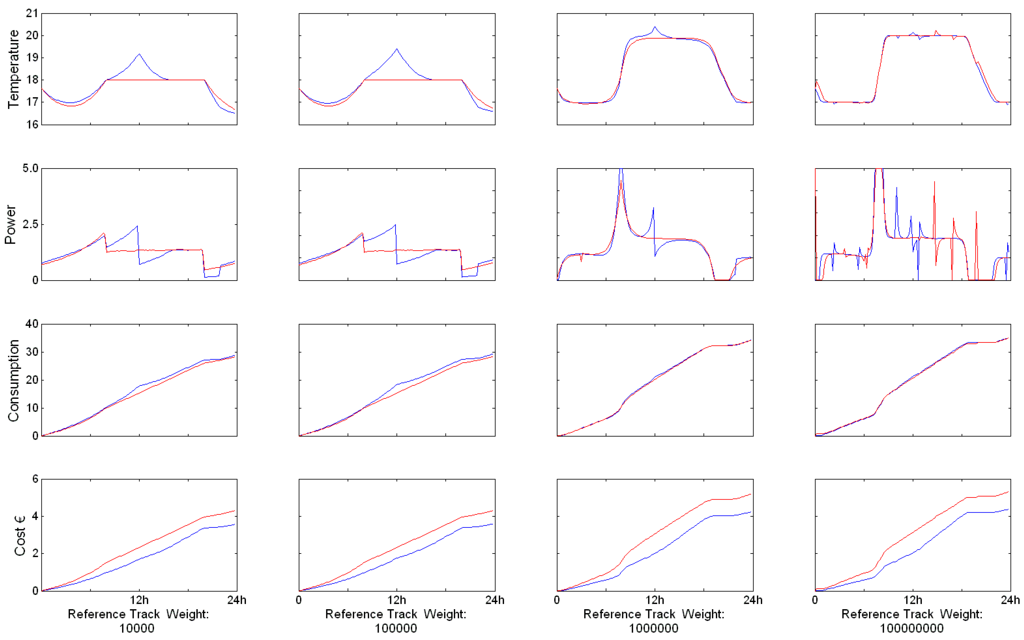
4.4. Economic Impact

In order to complete this study, the economic impact of the use of the MPC has been evaluated when a variable cost of the energy is considered. Given a TOU tariff of a local company, the comparison with the already studied thermostatic ON-OFF does not improve the consumption in a significant way. The MPC takes advantage of its predictive capacities before the tariff change and raises its consumption inducing a power peak that is dissipated after the change. This consumption peak is most valuable in buildings with large thermal inertia and it is fundamental for climate systems like Thermally Activated Building Systems (TABS). The weights of the cost functions vary inside the prediction horizons, in agreement with the tariff cost in that predicted moment of use. Besides, the reference temperature also varies within the prediction horizon. In order to develop the MPC, the CPLEX solver has been used with YALMIP so as to simulate the behavior of the dwelling under a Time of Use (TOU) tariff.
Comparing with an MPC of the same characteristics but with an invariable energy tariff, economics savings have been observed for different MPC configurations. Figure 9 shows the action of two MPCs over the model of the dwelling during a day. Both of them have the same pattern for high-energy savings. However, while the blue one uses a TOU tariff, the red one has no kind of cost discrimination over time. The parameters of the electric rate that weigh the energy use in the cost function, Equation (9), are defined in Table 5. It can be seen how in this particular example there is not significant energy savings at the end of the day. Nevertheless, the consumption pattern is shifted over the time producing significant economic savings due to the use of the promoted tariff period.
Similar results may be observed from Figure 10 and Table 6 for different reference track weights. It may be seen that, while the consumption of energy is similar in both MPCs, the predictive behavior of the MPC allows a relevant economic savings using TOU tariffs. In order to decrease the effect of the economic parameters of the tariffs of the Table 5 and to focus the comparison in the control effect, the three column of Table 6 shows the answer of both controls under the economic effect of the TOU tariff. Economics savings can be attached due to the control action while the control is able to adapt the temperature inside the comfort band. Owing to the peak of consumption produced before the tariff rate change, an improvement in the comfort can also be observed.

5. Conclusions

The development of a MPC over the experimentally obtained RC model of a real dwelling has been performed in order to study its response and evaluate its possible implementation as a heating system control that satisfies a power-saving policy. The model under consideration deals with a dwelling that does not meet the European Energy Performance of Buildings Directive proposed standards due to its outdated design and materials.
The results of this study can be considered to be a novelty, since most of the research and implementation over MPC are developed in new construction emblematic buildings provided with high quality climate systems and materials.
Comparing the results with the ones obtained for ON-OFF thermostatic controls, the achieved energy savings vary between 10% and 15% of the consumption, which is similar to the ones reported in the literature for better quality buildings.
Although the experimentally obtained model of the dwelling can be considered to be simple, this characteristic can be used to understand the results of the study in a qualitative way more than in a quantitative one and take them as a soft reference for buildings of similar characteristics.
Differences between diverse policies in the weights of the MPC can suppose savings of the 7.5% of the use of energy, so defining a relaxed policy about the reference temperature but maintaining it inside the comfort band can yield important savings.
The economic savings of MPC respect to hysteresis ON-OFF controls come from the energy savings. A further economic study has been carried out when a TOU tariff is used. In this case, the MPC shifts the usage of energy towards the low cost period.
As a future research work, the study can be expanded by the introduction of different parameters of the thermal adaptive control and evaluate the thermal discomfort using PPD value as metric. A deviation between the model of the building used to deploy the control and the model over which the model acts can also be introduced adding a Kalman filter to the control.

Acknowledgments

The authors would like to acknowledge the collaboration of the Basque Energy Board (EVE) through Agreement UPV/EHUEVE23/6/2011 and the Spanish National Fusion Laboratory (CIEMAT) UPV/EHUCIEMAT08/190. Authors are also very grateful for the partial financial contribution to the UPV/EHU and EJ/GV through projects GIU14/07 and IT987-16, as well as to the FEDER and MINECO through project DPI2015-70075-R.

Author Contributions

All authors have been involved in the preparation of the manuscript.

Conflicts of Interest

The authors declare no conflict of interest.

Abbreviations

The following abbreviations are used in this manuscript:
ANN
Artificial Neural Network
ASHRAE
American Society of Heating, Refrigerating and Air Conditioning Engineers
CTSM-R
Continuous Time Stochastic Modelling package for R
ISO
International Standards Organization
LTI
Linear Time Invariant
MPC
Model Predictive Control
PPD
Percentage of People Dissatisfied
PMV
Predicted Mean Vote
PRSB
Pseudo-Random Binary Signal
RBC
Rule-Based Control
ROLBS
Randomly Ordered Logarithmically distributed Binary Sequence
TABS
Thermally Activated Building Systems
TOU
Time of Use

Appendix A

RC parameters of the dwelling as detailed in [19]:
C (MJ/K)R (K/W)
Structure29.411Rstr_11/8200.558
Rstr_21/1191
Rstr_31/1.8
Windows Rwin1/305 + 1/2550.007
Envelope1.975Renv11/12590.007
Renv21/338
Renv31/338
Renv41/1679
Heating System0.001Rh1/15.50.06
Air0.667
C is the thermal capacitance of the element and R its thermal resistance.

References

  1. European Commission. Energy Security Stress Tests, Security of Gas Supply, Infographic, 2014. Available online: http://ec.europa.eu/energy/stress_tests_en.htm (accessed on 15 January 2016).
  2. European Commission. EU Energy in Figures. Statistical Pocketbook 2014. 2014. Available online: http://ec.europa.eu/energy/observatory/statistics/statistics_en.htm (accessed on 15 January 2016).
  3. European Commission. The Energy-Efficient Buildings PPP: Research for Low Energy Consumption Buildings in the EU, 2014. Available online: http://ec.europa.eu/research/press/2013/pdf/ppp/eeb_factsheet.pdf (accessed on 15 January 2016).
  4. United Nations. Framework Convention for Climate Change Paris, 2015. Available online: http://unfccc.int/resource/docs/2015/cop21/eng/l09r01.pdf (accessed on 15 January 2016).
  5. Directive 2010/31/EU of the European Parliament and of the Council of 19 May 2010 on the Energy Performance of Buildings. Available online: http://eur-lex.europa.eu/LexUriServ/LexUriServ.do?uri=OJ:L:2010:153:0013:0035:EN:PDF (accessed on 15 January 2016).
  6. García, C.E.; Prett, D.M.; Morari, M. Model predictive control: Theory and practice—A survey. Automatica 1989, 25, 335–348. [Google Scholar] [CrossRef]
  7. Borrelli, F.; Bemporad, A.; Morari, M. Predictive Control for Linear and Hybrid Systems, 2015. Available online: http://www.mpc.berkeley.edu/mpc-course-material (accessed on 15 January 2016).
  8. Castilla, M.; Álvarez, J.D.; Normey-Rico, J.E.; Rodríguez, F. Thermal comfort control using a non-linear MPC strategy: A real case of study in a bioclimatic building. J. Process Control 2013. [Google Scholar] [CrossRef]
  9. Garrido, I.; Garrido, A.J.; Romero, J.A.; Carrascal, E.; Sevillano-Berasategui, G.; Barambones, O. Low Effort LI Nuclear Fusion Plasma Control Using Model Predictive Control Laws Mathematical Problems in Engineering, 2015. Available online: http://www.scopus.com/inward/record.url?eid=2-s2.0-84924530407&partnerID=40&md5=033c49cd1d4d33dadd615f87109a7c27 (accessed on 15 January 2016).
  10. Garrido, A.J.; Garrido, I.; Chalatsakos, O.; Vinas, A.; Villaverde, A.; Queral, V.; Romero, J.A. Modelling and control of the UPV/EHU stellarator, 2015. In Proceedings of the 23rd Mediterranean Conference on Control and Automation, Torremolinos, Spain, 16–19 June 2015; pp. 421–427. Available online: http://www.scopus.com/inward/record.url?eid=2-s2.0-84945905671&partnerID=40&md5=10726d35ca19d125f7cf9ea4cbe7d96f (accessed on 15 January 2016).
  11. Garrido, I.; Romero, J.A.; Garrido, A.J.; Lucchin, D.; Carrascal, E.; Sevillano-Berasategui, G. Internal inductance predictive control for Tokamaks. In Proceedings of the World Automation Congress, Waikoloa, HI, USA, 3–7 August 2014; pp. 628–633. Available online: http://www.scopus.com/inward/record.url?eid=2-s2.0-84908895118&partnerID=40&md5=8b0febfc32c2826d55834d7360f0b769 (accessed on 15 January 2016).
  12. Wallace, M.; Das, B.; Mhaskar, P.; House, J.; Salsbury, T. Offset-free model predictive control of a vapor compression cycle. J. Process Control 2012, 22, 1374–1386. [Google Scholar] [CrossRef]
  13. Wallace, M.; House, J.; Salsbury, T.; Mhaskar, P. Offset-free Model Predictive Control of a Heat Pump. Ind. Eng. Chem. Res. 2015, 54, 994–1005. [Google Scholar] [CrossRef]
  14. Široký, J.; Oldewurtel, F.; Cigler, J.; Prívara, S. Experimental analysis of model predictive control for an energy efficient building heating system. Appl. Energy 2011, 88, 3079–3087. [Google Scholar] [CrossRef]
  15. Ruelens, F.; Iacovella, S.; Claessens, B.J.; Belmans, R. Learning agent for a heat-pump thermostat with a set-back strategy using model-free reinforcement learning. Energies 2015, 8, 8300–8318. Available online: http://www.scopus.com/inward/record.url?eid=2-s2.084941710563&partnerID=40&md5=7fcf272d23477bbb15454ab2ad0b827d (accessed on 7 March 2016). [Google Scholar] [CrossRef]
  16. Collotta, M.; Messineo, A.; Nicolasi, G.; Pau, G. A dynamic fuzzy controller to meet thermal comfort by using neural network forecasted parameters as the input. Energies 2014, 7, 4727–4756. [Google Scholar] [CrossRef]
  17. Dragomir, O.E.; Dragomir, F.; Stefan, V.; Minca, E. Adaptive Neuro-Fuzzy Inference Systems as a strategy for predicting and controling the energy produced from renewable sources. Energies 2015, 8, 13047–13061. [Google Scholar] [CrossRef]
  18. Marvuglia, A.; Messineo, A.; Nicolosi, G. Coupling a neural network temperature predictor and a fuzzy logic controller to perform thermal comfort regulation in an office building. Build. Environ. 2014, 72, 287–299. [Google Scholar] [CrossRef]
  19. Garcia-Gafaro, C.; Escudero-Revilla, C.; Diarce, G.; Teres, J.; Odriozola, M. Caracterización térmica de viviendas a partir de monitorizaciones e identificación de parámetros. In Proceedings of VIII, CNIT Burgos, Spain, 19–21 June 2013; pp. 539–548.
  20. Van Dijk, H.A.L.; Téllez, F. Measurement and Data Analysis Procedures, Final Report of the JOULE II COMPASS project (JOU2-CT92-0216). 1995. [Google Scholar]
  21. Godfrey, K.R. Correlations methods. Automatica 1980, 16, 527–534. [Google Scholar] [CrossRef]
  22. Van der Heijde, B.; Carrascal Lecumberri, E.; Helsen, L. Experimental Method for the State of Charge Determination of a Thermally Activated Building System (TABS). In Proceedings of 13th International Conference on Energy Storage, IEA-ECES Greenstock, Beijing, China, 19–21 May 2015; Available online: https://www.researchgate.net/publication/277308406_Experimental_Method_for_the_State_of_Charge_Determination_of_a_Thermally_Activated_Building_System_TABS (accessed on 15 January 2016).
  23. CTSM-R Development Team. Continuous Time Stochastic Modeling CTSM: User’s Guide and Reference manual. Version 1.0.0. 2015. Available online: http://ctsm.info (accessed on 28 March 2016).
  24. Gutschker, O. Parameter identification with the software package LORD. Build. Environ. 2008, 43, 163–169. [Google Scholar] [CrossRef]
  25. De Coninck, R.; Magnusson, F.; Åkesson, J.; Helsen, L. Toolbox for development and validation of grey-box building models for forecasting and control. J. Build. Perform. Simul. 2015. [Google Scholar] [CrossRef]
  26. TRNSYS 17: A Transient System Simulation Program; Solar Energy Laboratory, University of Wisconsin: Madison, WI, USA, 2010; Available online: http://sel.me.wisc.edu/trnsys (accessed on 28 March 2016).
  27. EnergyPlus; U.S. Department of Energy (DOE). Available online: https://energyplus.net/ (accessed on 28 March 2016).
  28. Gyalistras, D.; Gwerder, M. Use of Weather and Occupancy Forecasts for Optimal Building Climate Control (OptiControl): Two Years Progress Report; Technical Report; ETH Zurich and Siemens Building Technologies Division, Siemens Switzerland Ltd.: Zug, Switzerland, 2009. [Google Scholar]
  29. Gwerder, M.; Gyalistras, D.; Sagerschnig, C.; Smith, R.S.; Sturzenegger, D. Final Report: Use of Weather and Occupancy Forecasts for Optimal Building Climate Control—Part II: Demonstration (OptiControl-II); Automatic Control Laboratory, ETH Zurich: Zug, Switzerland, 2013; p. 156. [Google Scholar]
  30. Sourbron, M. Dynamic Thermal Behavior of Buildings with Concrete Core Activation. Ph.D. Thesis, KU Leuven, Leuven, Belgium, September 2012. [Google Scholar]
  31. Ashouri, A.; Petrini, F.; Bornatico, R.; Benz, M.J. Sensitivity analysis for robust design of building energy systems. Energy 2014, 76, 264–275. [Google Scholar] [CrossRef]
  32. KU Leuven and 3E. Open-IDEAS Source Code Repository, 2014. Available online: https://github.com/open-ideas (accessed on 15 January 2016).
  33. Åkesson, J.; Årzén, K.-E.; Gäfvert, M.; Bergdahl, T.; Tummescheit, H. Modeling and Optimization with Optimica and JModelica.org—Languages and Tools for Solving Large-Scale Dynamic Optimization Problems. Comput. Chem. Eng. 2010, 34, 1737–1749. [Google Scholar] [CrossRef]
  34. Lin, Y.; Middelkoop, T.; Barooah, P. Identification of control-oriented thermal models of rooms in multi-room buildings. In Proceedings of the 2012 IEEE 51st Annual Conference on Decision and Control (CDC), Maui, HI, USA, 10–13 December 2012.
  35. Verbai, Z.; Lakatos, A.; Kalmár, F. Prediction of energy demand for heating residential buildings using variable degree day. Energy 2014, 76, 780–787. [Google Scholar] [CrossRef]
  36. Gwerder, M.; Lehmann, B.; Tödtli, J.; Dorer, V.; Renggli, F. Control of thermally-activated building systems (TABS). Appl. Energy 2008, 85, 565–581. [Google Scholar] [CrossRef]
  37. Bacher, P.; Madsen, H. Procedure for Identifying Models for the Heat Dynamics of Buildings; Technical Report; IMM Technical University of Denmark DTU: Lyngby, Denmark, 2010. [Google Scholar]
  38. Bacher, P.; Madsen, H. Identifying suitable models for the heat dynamics of buildings. Energy Build. 2011, 43, 1511–1522. [Google Scholar] [CrossRef] [Green Version]
  39. Kristensen, N.R.; Madsen, H. Continuous Time Stochastic Modelling—Mathematics Guide; Technical University of Denmark DTU: Lyngby, Denmark, 2003; Available online: http://www.imm.dtu.dk/~ctsm/MathGuide.pdf (accessed on 15 January 2016).
  40. De Coninck, R.; Helsen, L. Practical implementation and evaluation of model predictive control for an office building in Brussels. Energy Build. 2016, 111, 290–298. [Google Scholar] [CrossRef]
  41. Verhelst, C.; Logist, F.; Impe, J.V.; Helsen, L. Study of the optimal control problem formulation for modulating air-to-water heat pumps connected to a residential floor heating system. Energy Build. 2012, 45, 43–53. [Google Scholar] [CrossRef]
  42. Maasoumy, M. Modeling and Optimal Control Algorithm Design for HVAC Systems in Energy Efficient Buildings. Master’s Thesis, University of California, Berkeley, CA, USA, February 2011. [Google Scholar]
  43. Sturzenegger, D.; Gyalistras, D.; Morari, M.; Smith, R. Semiautomated modular modeling of buildings for model predictive control. In Proceedings of the Fourth ACM Workshop on Embedded Sensing Systems for Energy-Efficiency in Buildings, Toronto, ON, Canada, 6 November 2012; pp. 99–106.
  44. CTE DB-HE 2013. Technical Building Code Basic Document-Basic Requirements Energy Saving; Ministry of Development: Madrid, Spain, 2013; Available online: http://www.codigotecnico.org/index.php/menu-ahorro-energia (accessed on 15 January 2016).
  45. Nicol, J.F.; Humphreys, M.A. Adaptive thermal comfort and sustainable thermal standards for buildings. Energy Build. 2002, 34, 563–572. [Google Scholar] [CrossRef]
  46. ASHRAE 55, Thermal Environmental Conditions for Human Occupancy; American Society of Heating, Refrigerating, and Air-Conditioning Engineers, ASHRAE: Atlanta, GA, USA, 2013; Available online: https://www.ashrae.org/resources--publications/bookstore/standard-55 (accessed on 7 March 2016).
  47. ISO 7730:2005—Ergonomics of the Thermal Environment. 2015. Available online: http://www.iso.org/iso/home/store/catalogue_tc/catalogue_detail.htm?csnumber=39155 (accessed on 7 March 2016).
  48. CPLEX Optimization Software Package. IBM. Available online: http://www-01.ibm.com/software/commerce/optimization/cplex-optimizer/ (accessed on 15 January 2016).
  49. Löfberg, J. YALMIP: A Toolbox for Modeling and Optimization in MATLAB. In Proceedings of the CACSD Conference, Taipei, Taiwan, 2–4 September 2004; Available online: http://users.isy.liu.se/johanl/yalmip/pmwiki.php (accessed on 15 January 2016).
  50. Cho, S.H.; Zaheer-uddin, M. Predictive control of intermittently operated radiant floor heating systems. Energy Convers. Manag. 2003, 44, 1333–1342. [Google Scholar] [CrossRef]
Figure 1. The building in Bilbao 43°15′30″N, 2°54′00″W.
Energies 09 00251 g001
Figure 2. RC-model of the dwelling.
Energies 09 00251 g002
Figure 3. RC model for parameter recognition.
Energies 09 00251 g003
Figure 4. Model Predictive Control (MPC) applied to the dwelling model, heat system consumption, outdoor temperature and solar radiation. Black line represents the temperature reference changes between 20 and 17 °C.
Energies 09 00251 g004
Figure 5. Three days zoom: Indoor temperature, heat power pattern, energy consumption and deviation respect the set point for heat system of 2.5 kW and 5.0 kW. Solid black line represents the variation of the temperature of reference.
Energies 09 00251 g005
Figure 6. Comparison between Model Predictive Control (MPC) and Hysteresis control. Indoor temperature, power consumption pattern, consumed energy and deviation from the setup for a 5-day period. Black line represents the temperature reference evolution.
Energies 09 00251 g006
Figure 7. System response for different weight relation (ΔReference:Control). Black Line represents the variations of the temperature of reference.
Energies 09 00251 g007
Figure 8. Variation of the control horizon respect a fixed prediction horizon (prediction:control). Black Line represents the variations of the temperature of reference.
Energies 09 00251 g008
Figure 9. One-day comparison of two energy savings oriented Model Predictive Controls (MPCs).
Energies 09 00251 g009
Figure 10. One-day for a comparison between a Time of Use (TOU) tariffed (blue) and no time discriminative (red) Model Predictive Control (MPC) for different weight relations. Indoor temperature (°C), Power use pattern (kW), total consumption (kW·h) and economic cost (€) are represented row wise.
Energies 09 00251 g010
Table 1. Hysteresis band definition for the ON-OFF controls.
HysteresisDayNight
Upper LimitLower LimitUpper LimitLower Limit
hys_HARDTref + 0.1 °CTref − 0.1 °CTref + 0.1 °CTref − 0.1 °C
hys_SOFTTref + 2 °CTref − 2 °CTref + 1 °CTref − 1 °C
Tref is 20 °C by day and 17 °C by night.
Table 2. Weight values used in the Model Predictive Controls (MPCs).
MPCWeight for (ω − θin) Q (1/K2)Weight for u R (1/W2)
MPC_HARD10,0001
MPC_SOFT401
Q and R are the weights for the deviation from the reference temperature, (ω − θin), and power use, u, applied in the cost function, Equations (6) or (9), to characterize the control.
Table 3. Energy consumption in February.
ControlEnergy Consumption (kW·h)
hys_HARD700
hys_SOFT692.125
MPC_HARD639.070
MPC_SOFT596.322
Table 4. Energy consumption in February for different weight relations.
Weight Relation Q:REnergy Consumption (kW·h)Hours of Thermal Discomfort (h·K)
10,000:1636.6810
1000:1623.9140
40:1584.8480
10:1547.62520.12
1:1542.67861.32
Q and R are the weights applied in the cost function, Equation (6) or (9), to the deviation between the reference and the real temperature and the power consumption respectively.
Table 5. Considered Time of Use (TOU) and no discriminative tariff for the economic study of the Model Predictive Control (MPC).
TOU TariffNo Discriminative Tariff
Peak 12:00 a.m.–22:00 p.m.Valley 22:00 p.m.–12:00 a.m.
0.17977 €/kW·h0.09572 €/kW·h0.15207 €/kW·h
Table 6. Economic savings in February between Time of Use (TOU) and no discriminative tariff (Table 5) for different weight relations between reference tracking and energy use.
Reference Tracking WeightEconomic Savings% (TOU vs. No Discriminative)Economic Savings% (TOU vs. No Discriminative with TOU Tariff)
10,000~19%~4.2%
100,000~18%~4.25%
1.0 × 10⁶~20%~4.2%
1.0 × 10⁸~19%~0.5%

