Article

Assessing the Potential of Plug-in Electric Vehicles in Active Distribution Networks

1
Department of Energy Technology, Aalborg University, Pontoppidanstraede 101, Aalborg 9220, Denmark
2
NEC Laboratories America Incorporations, Cupertino, CA 95014, USA
3
Electrical and computer engineering department, Montana State University, Bozeman, MT 59717, USA
*
Author to whom correspondence should be addressed.
Energies 2016, 9(1), 34; https://doi.org/10.3390/en9010034
Submission received: 23 October 2015 / Revised: 23 December 2015 / Accepted: 29 December 2015 / Published: 7 January 2016

Abstract

:
A multi-objective optimization algorithm is proposed in this paper to increase the penetration level of renewable energy sources (RESs) in distribution networks by intelligent management of plug-in electric vehicle (PEV) storage. The proposed algorithm is defined to manage the reverse power flow (PF) from the distribution network to the upstream electrical system. Furthermore, a charging algorithm is proposed within the proposed optimization in order to assure PEV owner’s quality of service (QoS). The method uses genetic algorithm (GA) to increase photovoltaic (PV) penetration without jeopardizing PEV owners’ (QoS) and grid operating limits, such as voltage level of the grid buses. The method is applied to a part of the Danish low voltage (LV) grid to evaluate its effectiveness and capabilities. Different scenarios have been defined and tested using the proposed method. Simulation results demonstrate the capability of the algorithm in increasing solar power penetration in the grid up to 50%, depending on the PEV penetration level and the freedom of the system operator in managing the available PEV storage.

1. Introduction

Inevitable presence of renewable energy sources (RESs) in modern power system has led to significant changes in different operation, protection, and management aspects of power systems. The distribution network plays a major role in the system overall performance, as it is the interface between the customers and the electric network. The main purpose of the network in the traditional power system was to respond to the customers’ demand anytime, no matter the circumstances. However, the improving and wide acceptance of RESs technologies in the last decade required new concepts for the design and operation of distribution networks, their functionality, and the role of customers in the new electric network paradigm [1]. The availability of RES for household application has changed the traditional customers to “prosumers”, where a customer can be a producer as well [2]. This paradigm shift introduces new opportunities as well as new challenges for the grid operation. In the future power system, each prosumer will be able to sell the excess available power to the upper grid, if requested, as a part of ancillary services [2]. However, new functionalities lead to certain challenges for grid operators, such as the unidirectional structure of the existing distribution networks [3,4], and voltage issues in the grid [5,6]. Therefore, optimal sizing and siting of RESs in distribution networks has received significant interest in recent years. An optimal placement of distributed generation (DG) units is discussed in [7,8] to reduce network losses. Lin et al. [9] proposes an optimization algorithm for photovoltaic (PV) penetration in distribution systems in order to maximize the net present value (NPV) of PV panels. An optimization algorithm based on a genetic algorithm (GA) was proposed in [10], with the main objective of maximizing the savings in the system upgrade investment deferral, and minimizing cost of annual energy loss. On the other hand, increasing interest in plug-in electric vehicles (PEVs), especially PEVs with lithium-ion (Li-ion) storage, has led to a huge interest in application of PEVs for grid support and ancillary services. The main role of ancillary service is to enable the system operator to deal with balancing issues. PV generation is variable and non-dispatchable. Therefore, its application in ancillary service depends on the availability and application of storage devices. The application of PEVs can be beneficial to overcome a part of inherent variability of PV generation, and also to improve the applicability of distributed RES for ancillary services [11]. Different research works have addressed the PEV potential for grid support [11,12,13,14,15,16,17,18,19,20]. On the other hand, due to technology improvement and cost reduction, PEVs are becoming popular, imposing new loads on power system. The grid features are normally designed considering current (and the traditional future forecast) customers’ consumption. Therefore, the low voltage (LV) grid would face new challenges as PEVs add on to the grid. As a result, PEVs charging scheduling becomes important for system operators, and has attracted attention from many research groups [13].
In this paper, an algorithm is proposed based on optimal management of PEV storage, in order to maximize PV participation in ancillary services. This way, part of the required ancillary services will be provided by the PV panels installed in distribution networks to alleviate the system operational costs. In addition, the total power loss of the system is included in the optimization procedure, so that the system energy losses will also be minimized. Although an optimal placement of DGs has been proposed in [7,8], but the main objective in these literature was to minimize the network losses, and providing ancillary service has not been considered in their optimization. On the other hand, the proposed algorithm in [9] aims at maximizing NPV by optimizing the placement of PV panels in the network. Therefore, it does not consider ancillary service as its major objective, and network losses are not a big concern in this study. In addition, the proposed GA optimization in [10] aims at minimizing the system investment cost, as well as minimizing annual energy loss. On the other hand, most of the studies on PEVs, such as [13,15], are focused on optimal charging strategies, regardless of the potential of PEVs for grid support. In [16], a vehicle to grid (V2G) strategy has been discussed for PEVs, but the role of DGs has not been a major focus in [16].
A multi-objective optimization procedure is proposed to obtain the best viable solution for this purpose [21,22,23]. Appropriate voltage profile at different buses and the quality of service (QoS) for the PEV owners are among the major constraints in the proposed algorithm. Considering the physical constraints of electric equipment in the system, i.e., transformer nominal power and nominal currents of the cables, the problem formulation should take these limits into account as well. On the other hand, since the PEVs are utilized by the algorithm for grid support, the proposed algorithm should include a proper charging algorithm for PEVs to avoid any inconvenience for the PEV owners. The rest of the paper is organized as follows. Section 2 provides details of the proposed optimization method, together with algorithms and driving patterns proposed for electric vehicles (EVs). Section 3 explains the system modeling approach, including load, PV panels, and PEVs. Section 4 is dedicated to simulation results. Conclusions of the work results are presented in Section 5.

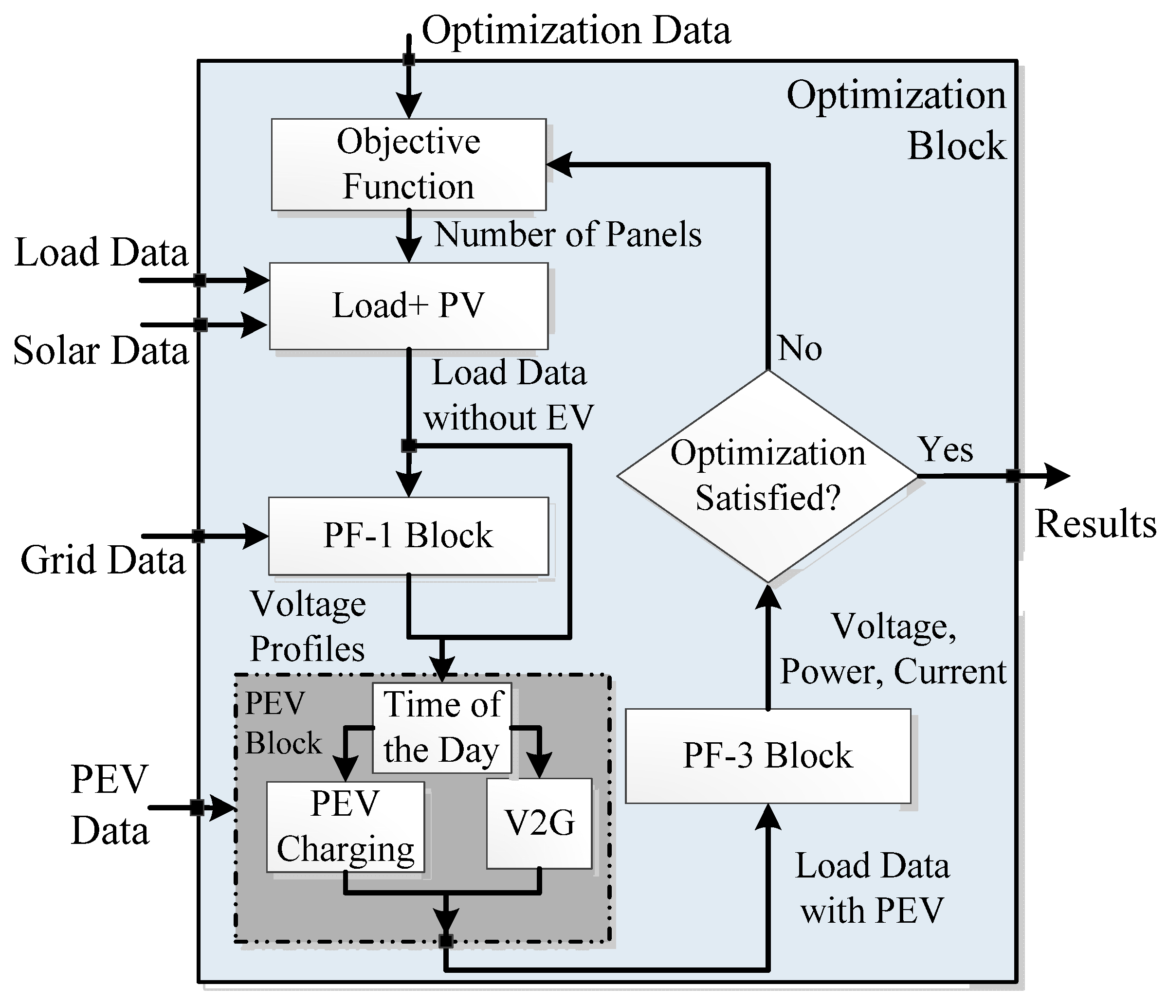
2. Proposed Intelligent Algorithm

The proposed optimization algorithm is presented in this section. A general overview of the LV grid is presented in Figure 1. In general, LV grids have a radial layout, and each distribution transformer is connected to four to seven LV distribution feeders. In this work, the 10 kV side of the grid is referred to as the “upper grid”, while the 0.4 kV side is considered the “LV grid”.
An overview of the proposed algorithm is shown in Figure 2. At the beginning, the “Objective Function” block generates optimization variables, “x”, i.e., number and locations of PV panels based on the optimization data. The generated PV sizes and locations along with solar irradiation and ambient temperature data will be utilized to prepare the power flow (PF) matrices. Then, the first PF study will be carried out to calculate the voltage magnitudes of different buses (PF-1 Block). The PF studies are based on Newton-Raphson load flow. The calculated voltages will be used in the PEV Block to compute PEV charging pattern, and PEV for grid support. Then, the load flow matrices will be modified based on the impact of the PEVs, and the load flow runs again (PF-3 Block). Finally, the required data for the Optimization Block will be calculated based on the recent load flow. In the following sub-sections, each block will be discussed in detail.
Figure 1. General layout of low voltage (LV) grid.
Energies 09 00034 g001
Figure 2. Proposed optimization method.
Energies 09 00034 g002

2.1. Objective Function

This block is responsible for finding “x”, i.e., the optimal number and location of the PV panels. Optimization data include the maximum and minimum number of panels that can be installed at each bus, and optimization technique parameters. The maximum number of panels is obtained by assuming that each household cannot install more than 2 units of “3 kW PV panel”. This is a fair assumption, considering the available roof area of a house. As a standard procedure for optimization problems, the first step is to define an appropriate objective function. Increasing the penetration of PV panels in the grid will lead to higher PF from the LV grid to the upper grid. Therefore, the main objective is to maximize the PF to the upper grid. This objective is defined as “f1” in Equation (3). Two other objectives are defined as minimizing the voltage deviation, represented by “f2”, and minimizing power losses, shown as “f3”. The voltage profile is known as an important operational index in the LV grids. In general, a multi-objective problem can be expressed as follows [21,22]:
minimize   F ( x ) :     F ( x ) = [ f 1 ( x ) , f 2 ( x ) , ... , f k ( x ) ]                       K =    3 subject to :    h j ( x ) 0   ;       ;       j = 1 , 2 , ... , n    
where “n” is the number of inequality constraints, and K is the number of objective functions. Here, “x” represents the optimization variables. In this work, the optimization variables are the number of PV panels on different grid buses, as presented in Equation (2):
x = [ x 1 , x 2 , ... , x q ]
In Equation (2), “q” represents the total number of buses in the grid. As mentioned above, the number of PV panels on each household is limited between 0 and 2, due to the available rooftop area of a common house. Therefore, the number of PV panels on each bus is limited to the maximum number of PV panels that can be installed on all the households on the bus. If four households are connected to a bus, then the maximum number of PV panels on the bus would be limited to eight.
As mentioned above, three different objective functions are considered in this paper, i.e., K = 3. The first objective function, i.e., maximizing the PF from the LV grid to the upper grid, can be equivalently replaced by minimizing the power from the upper grid to the LV grids, as follows:
f 1 ( x ) =   min    P T
In Equation (3), PT represents the PF through the transformer to the LV grid for the whole simulation period. In this work, the study was performed in 15 min time intervals, and the simulation was performed for a 24 h period. In other words, to obtain PT, PF through transformer is obtained for each simulation interval. Then, the average PF through the transformer for the whole simulation period (24 h) was obtained, i.e.,
P T =  mean   P trafo ( x )
The second objective is the voltage deviation among the grid buses, which can be obtained as follows:
f 2 ( x ) =   min    Δ V grid
where “∆Vgrid” is the maximum voltage deviation in the grid for the whole simulation time, as presented in Equation (6):
Δ V grid =  max  [ Δ V 1 , Δ V 2 , Δ V 3 , ... , Δ V b ]         b =    1 : q
In Equation (6), “∆Vb” represents the maximum voltage deviation of bus “b” during the whole simulation period. In this study, the study is performed for a 24 h time period, with 15 min time intervals, meaning that 96 time intervals have been defined for the study. Therefore, to calculate the maximum voltage deviation of bus “b” in Equation (6), “∆Vb”, voltage deviation of bus “b” is calculated in each time interval. Then, the maximum (i.e., worst) voltage deviation of bus “b” among the whole simulation time,”∆Vb”, is obtained, as presented in Equation (7):
{ Δ V b =    m a x    [ A b 1 , A b 2 .... , A bz ] ;    { z = 1 : 96 b     = 1 : q A bz = | V bz 1 |
In Equation (7), “b” represents the number of bus in the grid, and “z” represents the time interval of the study. As mentioned, this study is performed in 15 min time intervals, giving 96 time intervals for a 24 h case study. “Abz” is the voltage deviation of bus “b” (in p.u.) in simulation interval “z”. Minimizing the maximum voltage deviation amongst all buses guarantees that voltage deviations of other buses in the grid will also be minimized.
The last objective function is defined to minimize power losses (copper losses) in the grid, as expressed in Equation (8):
f 3 ( x ) = min    P loss,total
To obtain Ploss,total, the power loss of the whole LV grid is calculated at the end of each simulation interval. This value is obtained from the Newton-Raphson load flow of the grid. Then, total power losses of the grid for a day of simulation (i.e., Ploss,total) is computed by adding power loss values of all intervals together.
Three inequality constraints are considered in this study, as explained below:
(1)
Voltage of all buses must stay within a specific limit:
A bz Δ V standard           { z = 1 : 96 b     = 1 : q
where “Abz”, “b”, and “z” are defined in Equation (7). On the other hand, ∆Vstandard is the standard (maximum) voltage deviation of grid buses, which is defined by the grid codes and regulations [24].
(2)
PF through the transformer must be less than transformer nominal power (transformer capacity), as presented in Equation (10):
P T P nominal
where PT is already presented in Equation (4). Here, Pnominal is the nominal power (capacity) of transformer.
(3)
Line currents should never exceed the nominal currents of the cables:
i line i cable
In Equation (11), icable is the nominal current of the cables in the network, which is obtained from the network data. In addition, the line current, iline, is calculated from the Newton-Raphson load flow.
The multi-objective optimization can be solved in different ways, such as Pareto optimality methods [21], and weighting methods. In weighting methods, different objective functions can be combined into a single function with different weights. One of the weighting methods, known as the “Rank Order Centroid” (ROC) approach, is used in this work [22]. In this method, different objective functions are weighted and added to each other to form the single objective function as follows:
 min  s = 1 K w s f s ( x )       subject  to:    s = 1 K w s = 1
where “fs(x) is the sth objective function and “K” is the total number of objective functions, “K = 3”. In this work, the weight factors for functions “f1”, “f2”, and “f3” are 11/18, 5/18, and 2/18, respectively. In this paper, a heuristic method (specifically a GA) is used since the objective functions and constraints are nonlinear [23]. Details of the GA parameters are presented in Table A1 in Appendix A.

2.2. “Load + Photovoltaic” Block

This block prepares bus and line data matrices based on grid topology and grid demand data. Bus data, which contain generation and load data at each bus, will be modified based on the generated PV sizes and locations by the Optimization Block. Therefore, it is primarily required to calculate PV generation based on irradiation and ambient temperature.

2.3. Power Flow-1 Block

“PF-1 Block” represents a Newton-Raphson load flow study for the grid. In this study, the voltage level of different grid buses, in presence of PV panels, is used to design a charging/discharging algorithm for the PEVs in order to increase PV penetration and support the upper grid. Once the PV generation is too much, voltage at the bus of connection (and probably at the neighbor buses) shows undesired increase. On the other hand, LV at different buses shows deficiency of power, which can be compensated by PEV discharging, if available. Thus, the voltage magnitudes at different buses should be obtained before the utilization of PEVs. The “PF-1 Block” takes the data and calculates voltage magnitudes for the next time interval, using Newton-Raphson load flow [25].

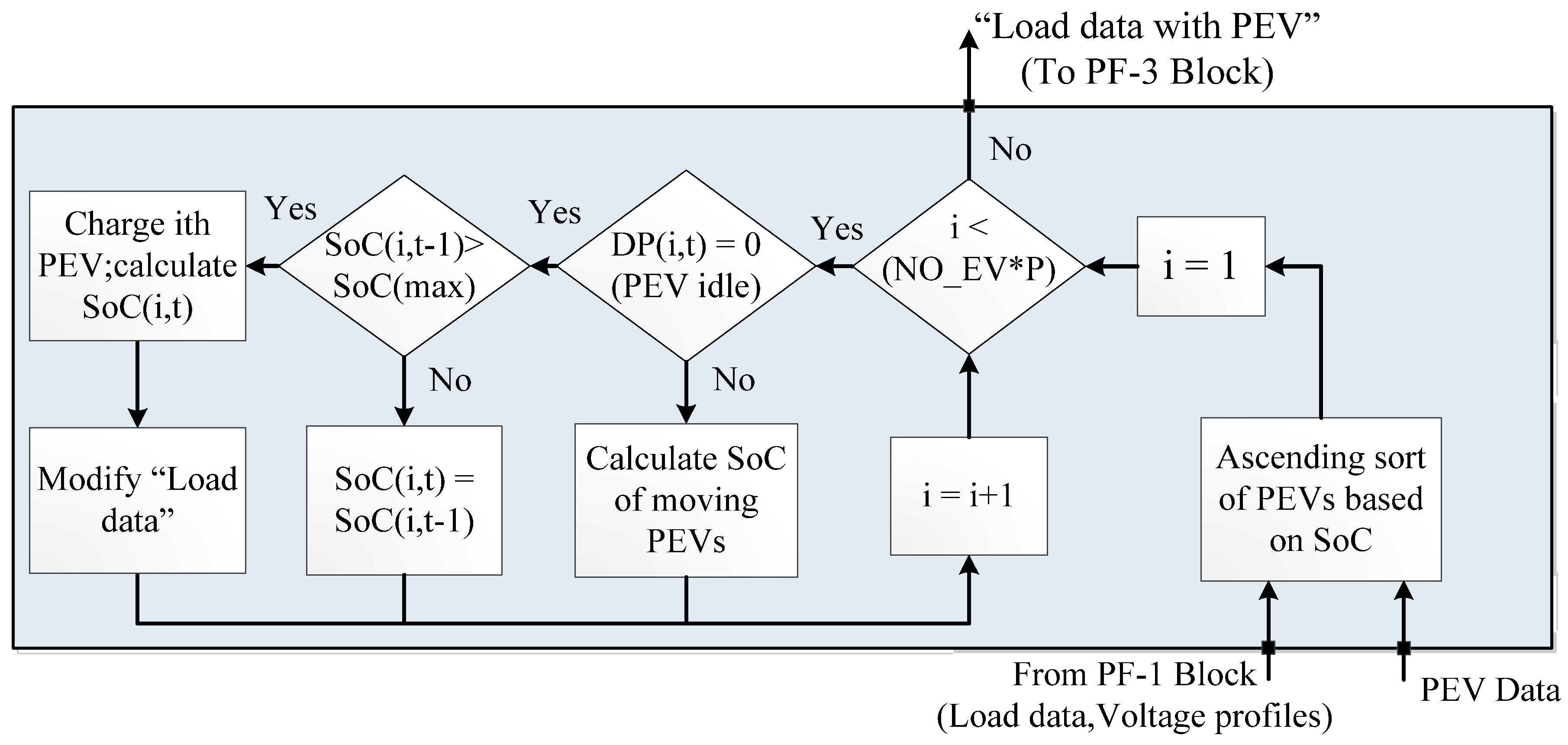
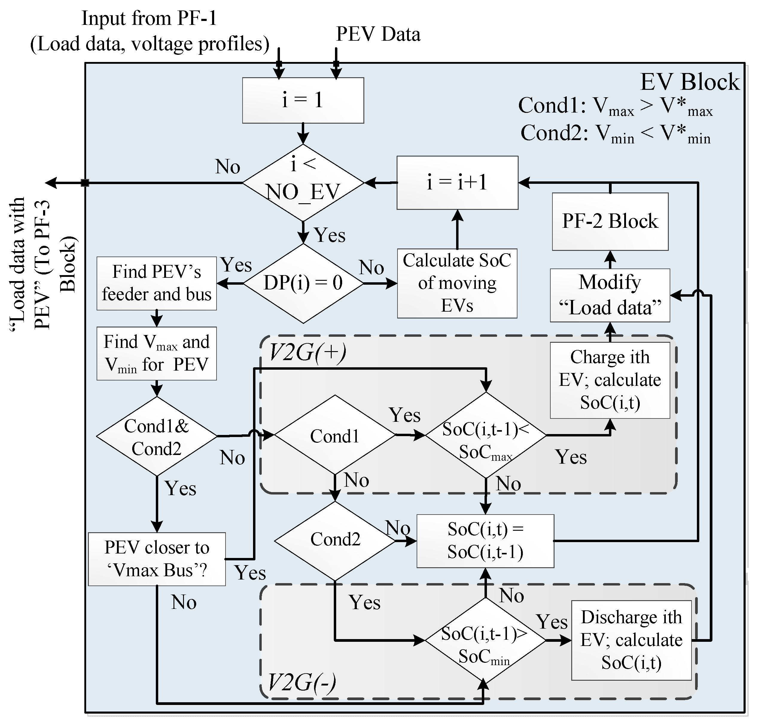
2.4. Plug-in Electric Vehicle Block

The “PEV Block” is responsible for computing the charging/discharging pattern for the PEVs based on their distance profile (DP) and the grid condition at each interval. The block receives PEV data and voltage magnitudes at different buses as the input. The PEV data includes: (1) the number and type of PEVs; (2) PEVs’ battery size; (3) initial state of charge (SoC) of PEVs at the beginning of simulation; (4) average consumption of different PEVs (Wh/km); (5) DP of PEVs; (6) nominal power of PEV charger; and (7) PEV buses with the number and types of PEVs on each bus. The SoC of PEVs changes during the day with respect to their DP and their average energy consumption. Therefore, in order to define a proper algorithm for PEVs, it is necessary to calculate the SoC of each PEV at the end of each interval. If the PEV is moving, the new SoC at the end of the interval will be calculated based on the PEV’s driving distance for that interval, type of PEV, its previous SoC, and its battery capacity. Otherwise, when the PEV is idle, its SoC does not change. The SoC will be calculated within “PEV Block” in Figure 2. From Figure 2, the “PEV Block” includes two individual blocks, “PEV Charging” and “V2G”. The reason is that a day of simulation is divided into two different blocks: (1) high irradiation and (2) low irradiation. The reason for the division is to find appropriate set points for the algorithm. The high solar irradiation and solar production during the daytime increases grid voltage levels, especially during the daytime. However, the solar production reaches zero during the evening and night hours. Therefore, different set points are defined for the algorithm to efficiently charge the PEV battery for customer requirements in the morning, while enabling the grid to utilize PEV storage for grid support.

2.4.1. Plug-in Electric Vehicle Charging

Considering the number of PEVs in the LV grid and their significant power demand, especially at night when most PEV owners plug their car for charging, a huge amount of load will be imposed on the grid which can result in voltage issues, as well as overcurrent in the lines and transformer. Therefore, a proper algorithm is required to handle PEV charging appropriately. Figure 3 presents the flowchart of the proposed algorithm for PEV charging. From Figure 3, all the PEVs connected to the grid will be sorted in ascending order based on their available SoC from the last interval. Sorting PEVs will enable the algorithm to charge certain PEVs with the least SoCs for simultaneous charging. After selecting the PEVs, each selected PEV will be examined for charging. If the ith PEV is moving (i.e., DP(i,t) ≠ 0), it cannot be charged and the algorithm only calculates its SoC at the end of the current interval. Otherwise, the PEV’s SoC at the end of the last interval will be evaluated, i.e., SoC(i, t − 1). If the PEV’s SoC is above SoCmax, the algorithm does not charge the PEV. This way, the SoC at the end of the current interval will be equal to its SoC from the last interval, i.e., SoC(i, t) = SoC(i, t − 1), because internal battery discharging is neglected in this study. Once the SoC of the ith PEV is less than SoCmax, the PEV will be charged. Here, the PEV’s SoC at the end of the charging period will be calculated and the “load data” matrix will be modified, due to PEV charging impact.
Defining a maximum value for battery charging (SoCmax) is due to battery lifetime issues [17]. Furthermore, the random displacement of different PEVs in different feeders and different buses enhance the algorithm performance and voltage profile at different buses, as it minimizes the probability of simultaneous charging of too many PEVs at the same feeder. The random placement of PEVs is performed only once at the initialization of the whole optimization program. Additionally, when the number of PEVs increases, the random selection nature of the proposed algorithm helps to keep the diversity for PEV selection, which results in higher probability of available PEV for charging at different buses at any time.
Figure 3. Charging pattern for plug-in electric vehicles (PEVs) for each interval of simulation.
Energies 09 00034 g003

2.4.2. Vehicle-to-Grid

PEVs utilization is a random behavior because of human interaction as the driver. This way, the PEV’s SoC at the end of each trip, charging and discharging preferences of the owner, and connectivity to the grid during the idle periods brings a new level of uncertainty in the power system. This results in higher operational cost due to the required ancillary services. In this study, the PEV behavior is represented by generating random driving patterns, selecting the type and their random displacement in the grid. The random driving patterns are produced with respect to statistical driving data provided by authorities. Two types of cars are considered in this study: commuters and family cars. Details of the PEVs are presented in Section 3. Commuters are mainly used in the morning and evening time, for travelling between home and work. Therefore, their driving pattern is mainly in the morning and evening time, and they are idle for most of the daytime. On the other hand, family cars have a more diverse driving pattern, as they will be used during the day more frequently. However, family cars are mainly used for short trips. Therefore, their battery charge does not change drastically. Further details on the driving patterns of PEVs are presented in Section 3.
Considering the driving patterns of PEVs and their idle time, when the PEV is idle and connected to the grid, the grid can benefit in two ways: (1) positive balance, where the storage capacity of PEV can be used to store extra energy [12]; and (2) negative balance, where the PEV can support the upper grid [17]. It should be noted that a PEV can be used for grid support only when: (1) the PEV is idle; (2) the PEV is connected to the grid; and (3) the PEV battery is available for such function. Due to the battery lifetime issues, batteries should not be charged more than a certain level (90%) [17]. On the other hand, batteries should always have a minimum level of charge to respond to the owners’ requirements. Thus, battery availability is limited to certain “minimum” and “maximum” values. Determining “minimum” value can be done considering PEVs’ DP and their daily distance. Figure 4 presents the proposed algorithm for such functions. For each interval, PEVs’ data (including locations, DP, and initial SoC) are given to the PEV Block (Figure 2 and Figure 4). Then, each PEV will be examined for its potential for grid support based on different rules and constraints. Since charging and discharging of PEV could affect the voltage of the whole feeder, the proposed algorithm is designed to consider voltage of the feeder to which PEV is connected.
Figure 4. Proposed algorithm for vehicle to grid (V2G) application of electric vehicles (EVs).
Energies 09 00034 g004
In the first iteration, the maximum and minimum voltage of the feeder (Vmax and Vmin, respectively) will be determined based on the data from PF-1 Block. However, for the next iterations these values will be determined by “PF-2 Block”, shown in Figure 4. “PF-2 Block” is also based on Newton-Raphson load flow calculations. Then, the obtained Vmax and Vmin will be compared with predefined set points, “V*max” and “V*min”. If ”Vmax > V*max”, named as “Cond1” in Figure 4, then the “V2G(+)” scenario applies. On the other hand, if “Vmin < V*min”, which is shown by “Cond2” in Figure 4, then the “V2G(−)” scenario is valid. For cases where both “Cond1” and “Cond2” criteria could happen, the decision is made based on the distance of the PEV from the buses. These scenarios are further explained below:
Scenario 1 (charging and discharging): If both maximum and minimum voltages of the feeder at hand are beyond the thresholds, which might happen if the feeder is too long and there are many PV panels installed at certain buses, priority between discharging and charging is given to the one that the PEV bus is closer to. As a result, discharging is preferred if the bus with minimum voltage is closer to the current PEV (D_Vmin < D_Vmax). Conversely, if the bus with maximum voltage is closer to the current PEV bus, then charging will be preferred (D_Vmax < D_Vmin). The desired operation on the PEV, however, depends on its availability and its SoC level.
Scenario 2 (only charging): If the maximum voltage is higher than a threshold (Vmax) in the whole feeder, there is an excess power generated by the PVs in that feeder which can be possibly stored in the PEVs. Thus, the current PEV will be examined to store the excess power. However, charging happens only if the PEV is idle and its battery SoC is less than the technical upper limit, i.e., 90% of its nominal capacity.
Scenario 3 (discharging): If the minimum voltage of the feeder is below Vmin, a shortage in the generation will be recognized. In this condition, the PEV will be examined for discharging based on its availability and SoC level.
Scenario 4: If the maximum and minimum voltages are within the pre-defined values, and the PEV is idle, the SoC of the PEV does not change.
In all scenarios (except Scenario 4), the bus matrix should be modified for the new Newton-Raphson PF in the “PF-3 Block”. This procedure will be done for all intervals of all PEVs.

2.5. Power Flow-3 Block

In this block, the modified “load data” matrix, considering charging and discharging operation of PEVs for the length of simulation, along with line matrix will be utilized to calculate new steady-state operating points. A similar PF structure, similar to PF-1 Block (i.e., Newton-Raphson-based PF), is used in this block; and only the loads have changed. Final load flow results will be utilized to calculate the required data for the Optimization in order to generate new solutions for the PV sizes and locations.

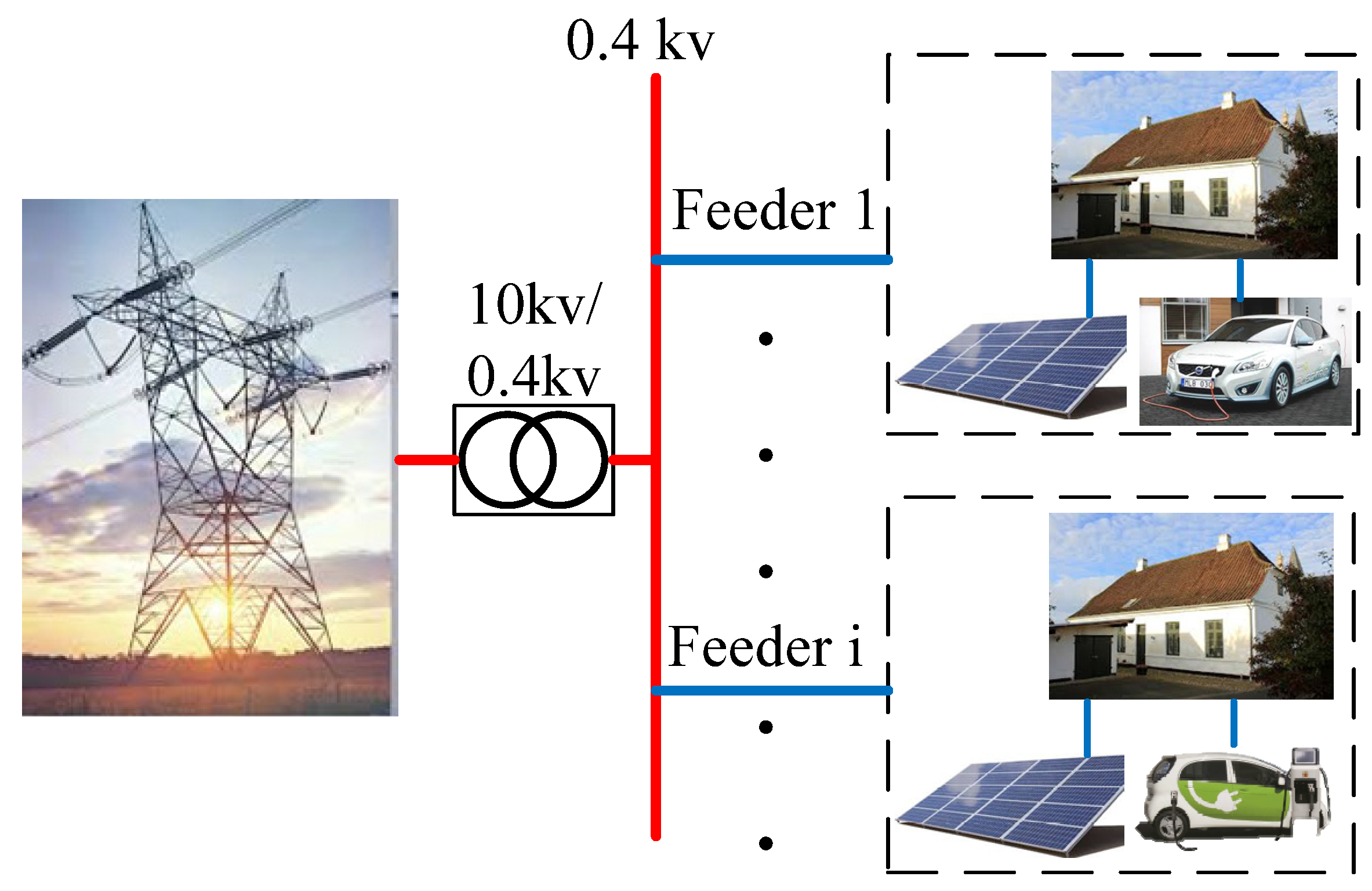
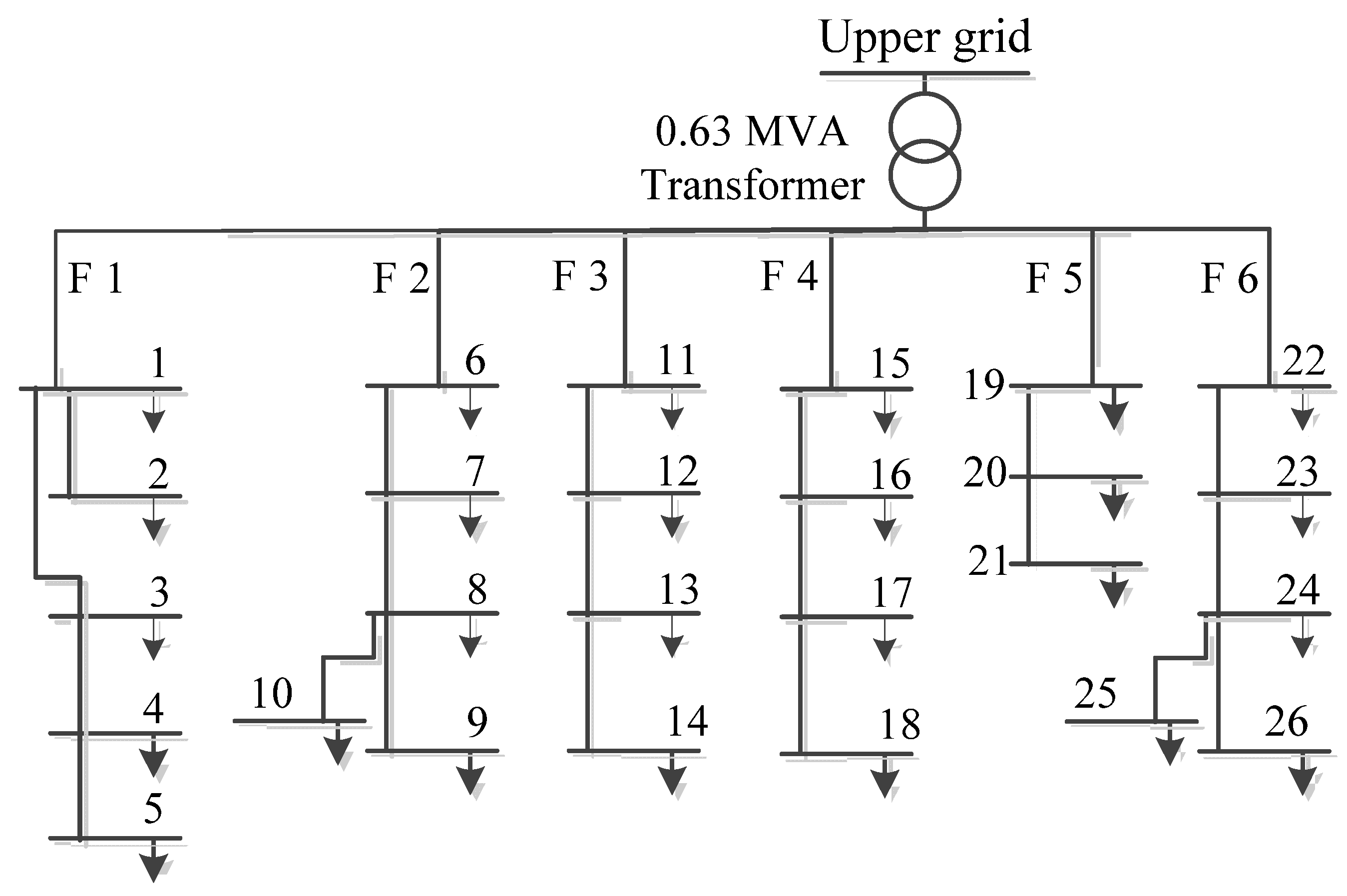
3. Grid Layout and Photovoltaic Modeling

The configuration of a Danish LV grid under study is shown in Figure 5. The LV grid has six feeders which are connected to a 20 kV/0.4 kV, 630 kVA distribution transformer. The number of households on each feeder is given in Table 1. The data of the cables are obtained using grid data presented in Table A2 in Appendix A [17,26]. For modeling PV panels, the model presented in [27] is applied. The only available datum in this study was the transformer load curve. Therefore, load modeling is done using the “Velander method”. This method is explained in [28,29]. This method is mainly used for studies where no measurement of single households in the grid is available. In this method, the power demand of the households will be obtained from the house’s “annual energy demand”.
Figure 5. Overall view of the LV grid.
Energies 09 00034 g005
Based on battery type and details required for a certain study, different models are proposed for PEVs [17,30]. In this study, PEVs with Li-Ion battery are considered since they are widely considered recently [31]. Besides, the PEVs’ DP, types, and their allocations in the grid should be defined. Although these parameters are not deterministic, a typical scenario is developed in this study to simplify it. Two types of PEVs are considered here: (a) commuters; and (b) family cars.
As mentioned in Section 2.4.2, two types of PEVs are considered in this study: commuters and family cars. In this study, the commuters and family PEVs have a 30 kW battery pack [32]. The required data for the PEVs are reported in Table 1 [32]. The main feature which differentiates PEVs is their average daily distance and owner behavior. To generate DP for PEVs, a random normal distribution is used. Based on the statistical data, commuters are mainly on the road in the morning, from 7:00 a.m. to 9:00 a.m., and during the evening time, from 5:00 p.m. until 7:00 p.m. Therefore, to provide a proper DP for commuters, their average daily distance (mentioned in Table 1) is split between morning and evening time intervals. The DPs of commuters are similar, except for a time shift for DPs of different commuters. On the other hand, family cars are used for short trips, while they have a more diverse moving time, depending on the needs of the car owner [32].
Table 1. Details of feeders and PEVs.
Number of households on grid feedersFeeder123456
No. of household203327281742
Details of PEVsPEV type% of PEVsBattery (kWh)Average consumption (Wh/km)Charger power (kW)Daily distance (km)
Commuter80301507.240
Family car20301507.225
The distribution of PEVs among feeders and buses depends on the number of the households on different buses, i.e., buses with higher number of households are likely to have higher number of PEVs. As a result, feeders with higher number of households will have higher number of PEVs connected to them. Such distribution of PEVs provides a more realistic scenario, since all the households are equally likely to own a PEV, regardless of their location on the LV grid.

4. Simulation Results

In this work, the nature of the optimization problem and variables (i.e., number of PVs) is an integer optimization. Usually, heuristic approaches are more effective than gradient-based techniques when it comes to nonlinear integer optimization. As a result, GA method is chosen for this study.

4.1. Case Studies

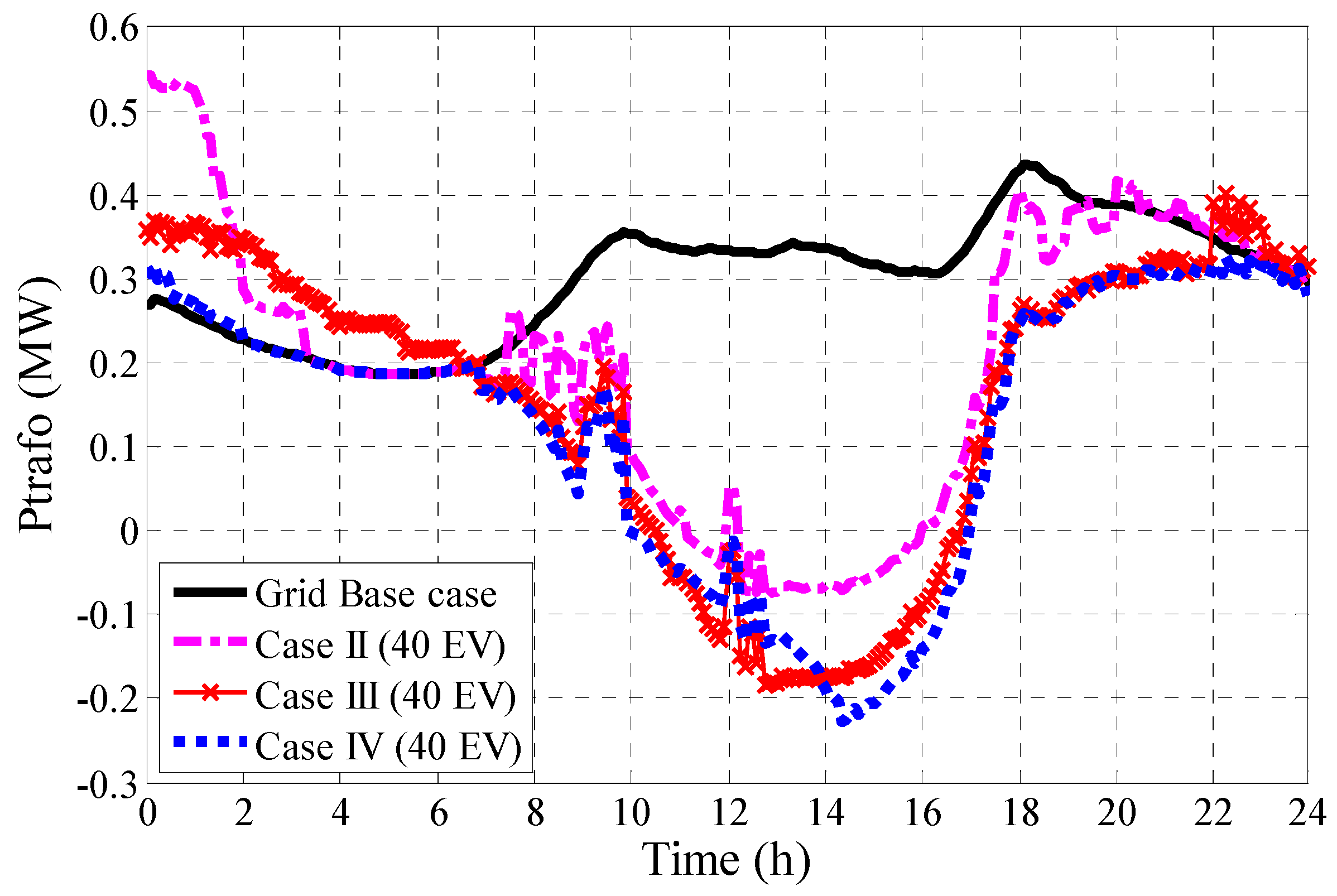
4.1.1. CASE I: Original Grid without Photovoltaic and Plug-in Electric Vehicle

First, the original grid is simulated with actual load demand without PV panels and PEVs. The data used in this simulation belong to the first day of July 2010. The reason for picking a summer day is the fact that solar irradiation becomes maximum in the summer. Therefore, it is better to determine the penetration level of solar panels in the summer. This way, it will be guaranteed that the solar power production never exceeds the grid limits. The solar irradiance also belongs to the same day of July 2010. The irradiation is obtained from a measurement device in the laboratory. As mentioned above, load modeling is performed using “Velander method”. The only available measurement for the grid was the power profile of transformer. Therefore, to provide a demand profile for the grid households, it is assumed that the demand profile of the grid households is similar to the demand profile of transformer.
The simulation reveals the possible issues with the grid which further can be utilized for comparison purposes. Voltages at some critical buses (i.e., at the end of the feeders) are shown in Figure 6.
Figure 6. Voltage profile of grid critical buses (no photovoltaic (PV) panels and no PEV).
Energies 09 00034 g006
Considering the standard voltage deviation limit [24], voltage violations at some buses can be recognized. Voltage violation is more severe for the end buses of feeders 2 and 6. The reason is the number of household on these feeders. It should be mentioned that, despite such voltage drop, such voltage profile is acceptable for Danish grid [24]. Since the “Velander” method is used for load modeling in this study, the voltage profiles obtained from simulations include more extremes comparing to the real situation. In reality, the voltage profiles in the grid have lower deviation and the voltage drop is also less than what is shown here.

4.1.2. CASE II: Optimization without Grid Support

In this case, it is assumed that the PEVs are considered as loads. PEVs are charged during the night time, using the smart charging algorithm, as presented in Figure 3. During the daytime, PEVs can only be used for positive balancing (from grid to vehicle). The goal of the optimization-based simulation is to find the optimal number and location of PV panels considering the new PEV loads. Typically, PEVs are under charge during the night hours, where the household demand is normally minimal. However, connection of a large number of PEVs to the feeder imposes a significant amount of load and leads to a significant voltage drop. To overcome this issue, the charging algorithm presented in Figure 3 is utilized. The lower and upper SoC of PEVs’ batteries are 20% and 90%, respectively.

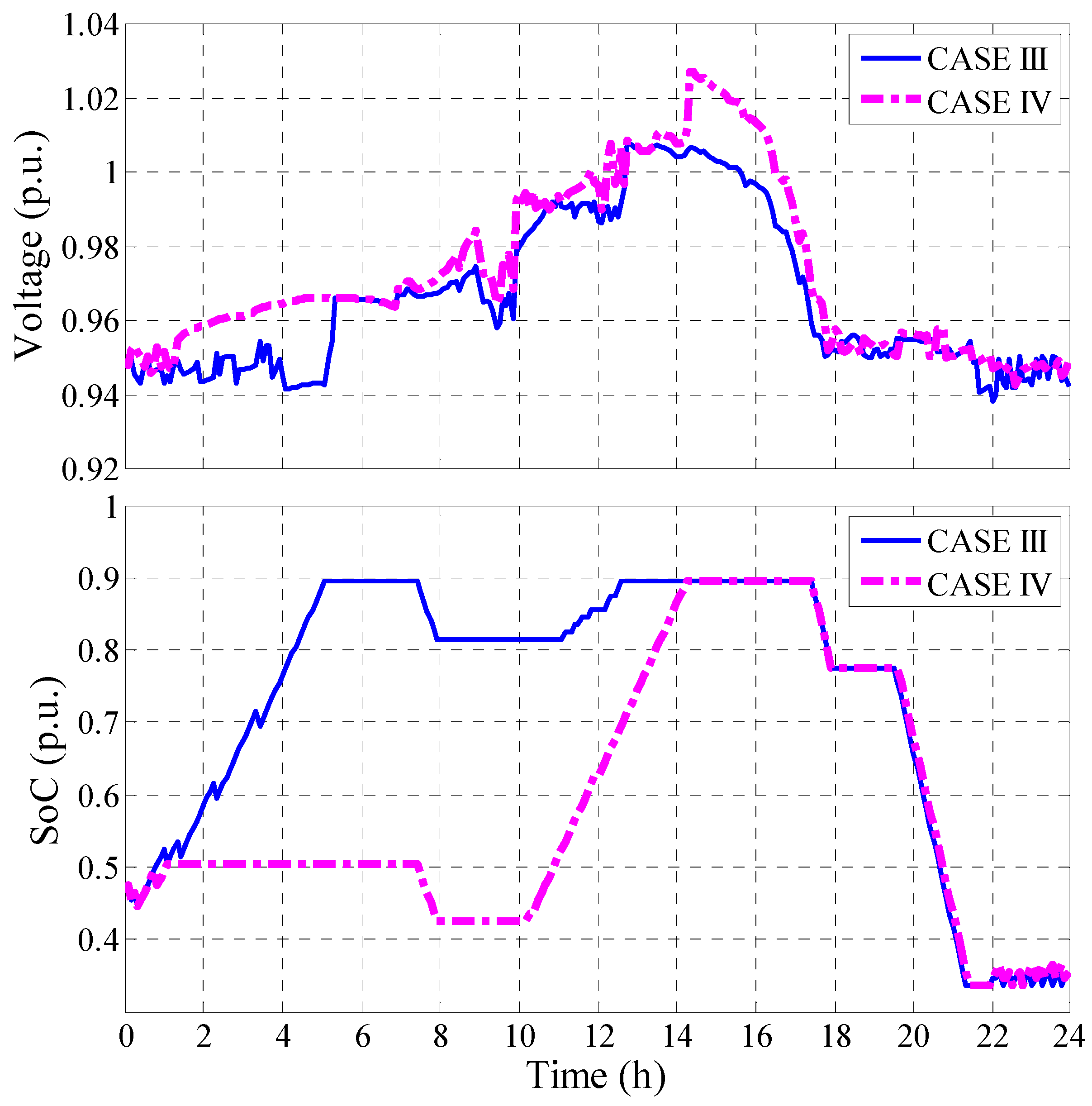
4.1.3. CASE III: Optimization Considering Grid Support

CASE III is similar to CASE II, except that the PEVs are utilized for V2G purposes (both positive and negative balance). Thus, CASE III contains the features of the proposed method in Section 2.4.2. Considering customer’s driving requirements, the lower limit of SoC is set to 35%, while the upper limit is 90% for night time charging, similar to CASE II.

4.1.4. CASE IV: Optimization Considering Grid Support

Case IV is similar to case III, but with a lower SoC limit during the night time. In other words, in order to increase the available PEV battery capacity for absorbing PV power during the daytime, it is assumed that the grid operator is allowed to restrict the upper limit of SoC for night-time charging to 50%. In such case, the available PEV storage for the daytime is higher.

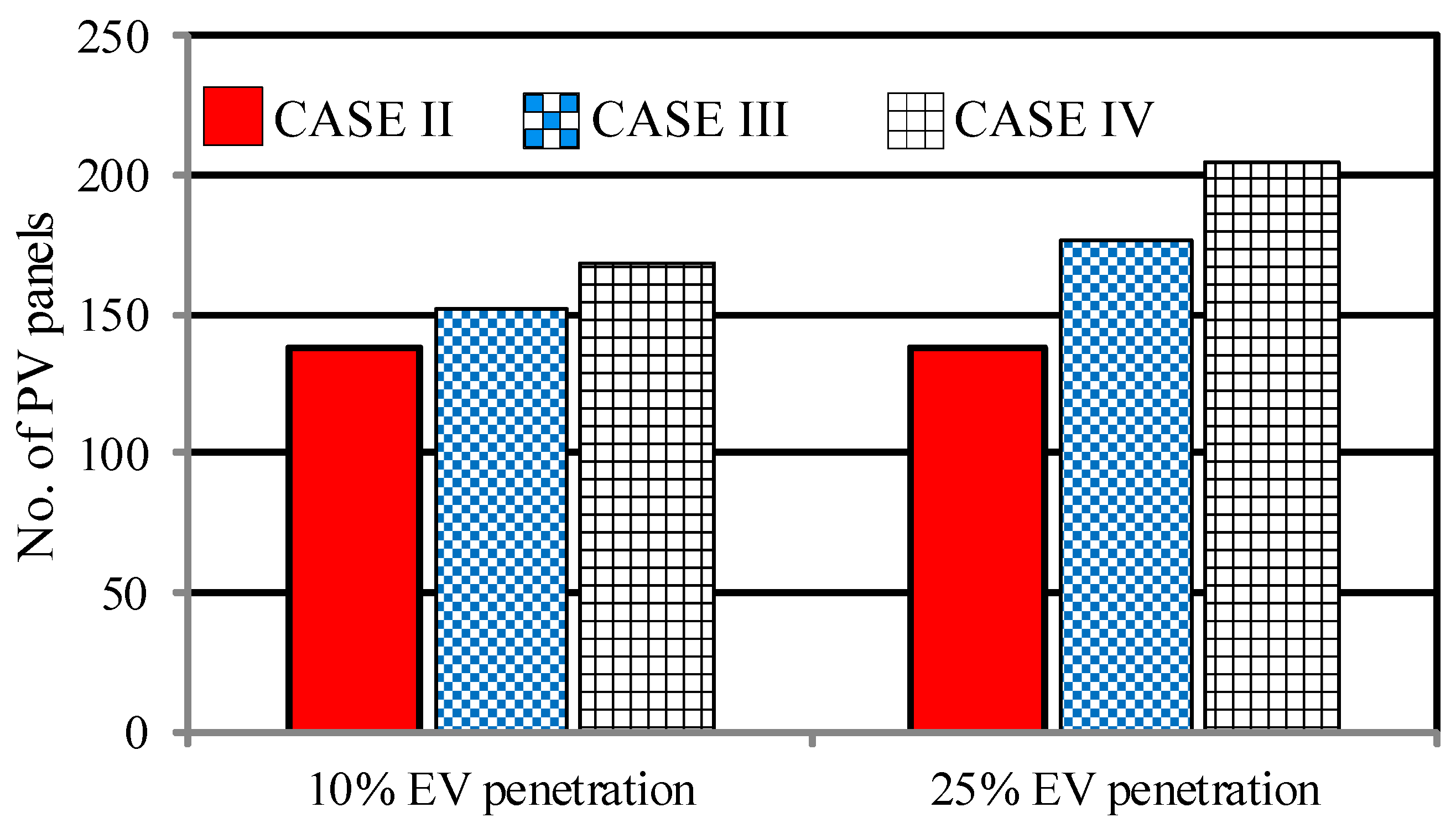
4.2. Optimization Results

In this section, simulation results of CASE II, CASE III, and CASE IV are presented. The number of PEVs in the LV grid was increased gradually to have the maximum PEV penetration. Here, the results with 16 PEVs (10% PEV penetration) and 40 PEVs (25% penetration) in the grid are presented. The optimization results are shown in Table 2.
To ease the comparison, the total number of PV panels for each case study is presented in Figure 7 as well. Considering the total number of panels for each case, the effectiveness of the proposed algorithm can be realized. Activating the negative balance option (i.e., discharging PEVs for grid support), for both CASE III and CASE IV, has led to a higher number of panels in the grid. Besides, in CASE IV, where the grid operator is allowed to limit the maximum charge of batteries (maximum 50% charging for the night time in this study), the number of panels has increased compared to CASE III. Such increase can be realized both with 10% PEV penetration, and with 25% PEV penetration, although the rate of increase is not the same. The reason for different rates is the fact that the placement of PEVs on different buses and the number of PEVs on different buses are not similar for the two cases. The maximum increase in the number of panels is in CASE IV with 40 PEVs in the grid (205 panels), which shows more than 32.7% increase compared to CASE II (138 panels). Since each panel’s nominal capacity is 3 kW, such increase is equal to 201 kW more PV panels.
Table 2. Number of PV panels for cases II–IV considering two PEV penetration levels: 10% and 25% PEV penetration.
BusCase IICase IIICase IV
10% (16 PEV)25% (40 PEV)10%25%10%25%
1222323
2666789
3113436
4444547
5334444
6666667
79910121112
82235610
9444667
10112446
11335868
12101010101010
13445658
14223546
15666666
16889101010
178899910
18888888
19101010101010
20888888
21888888
225568711
23667889
248888810
25555668
26111324
Total138138152177169205
Figure 7. Number of PV panels in different cases.
Energies 09 00034 g007

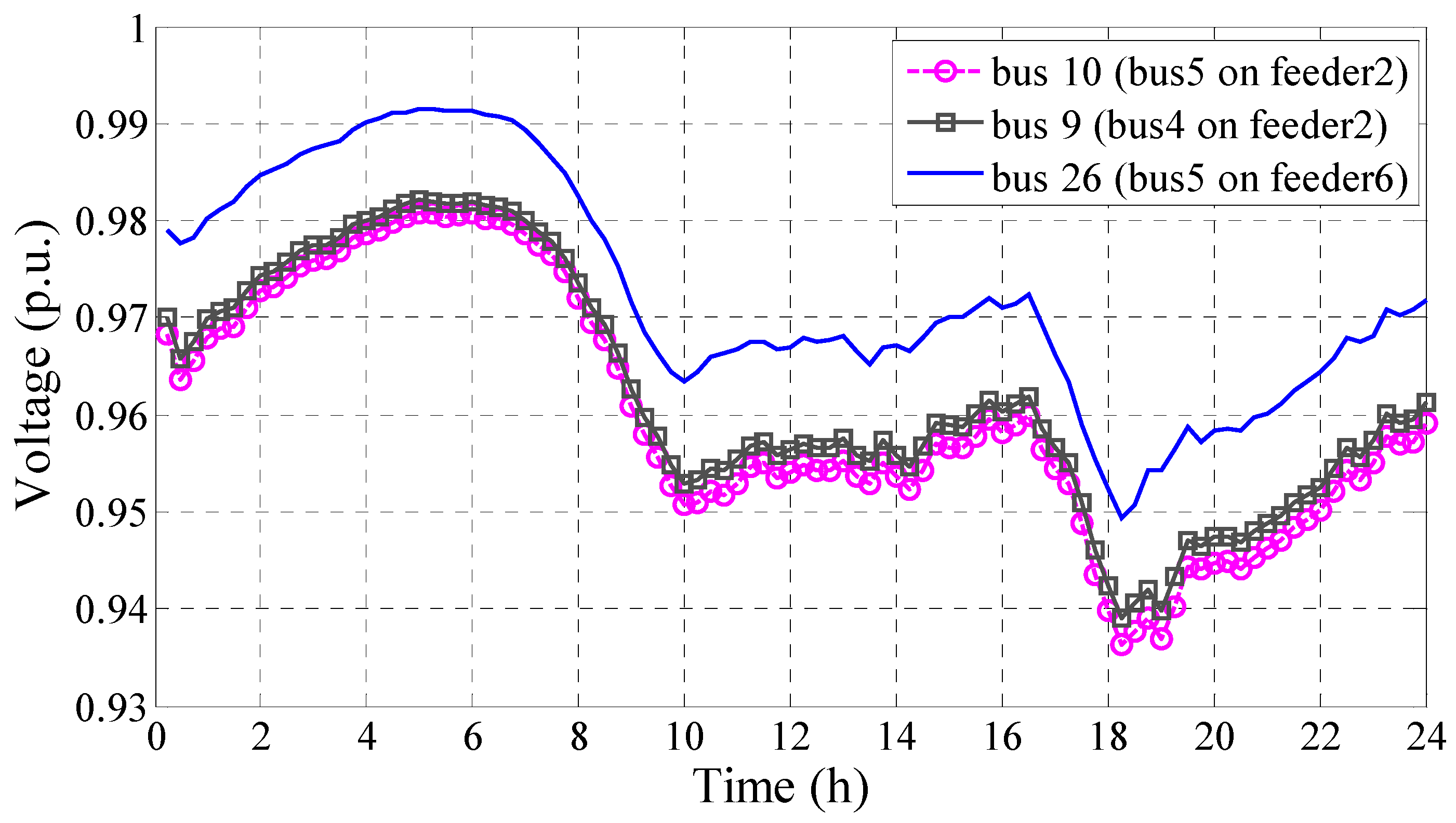
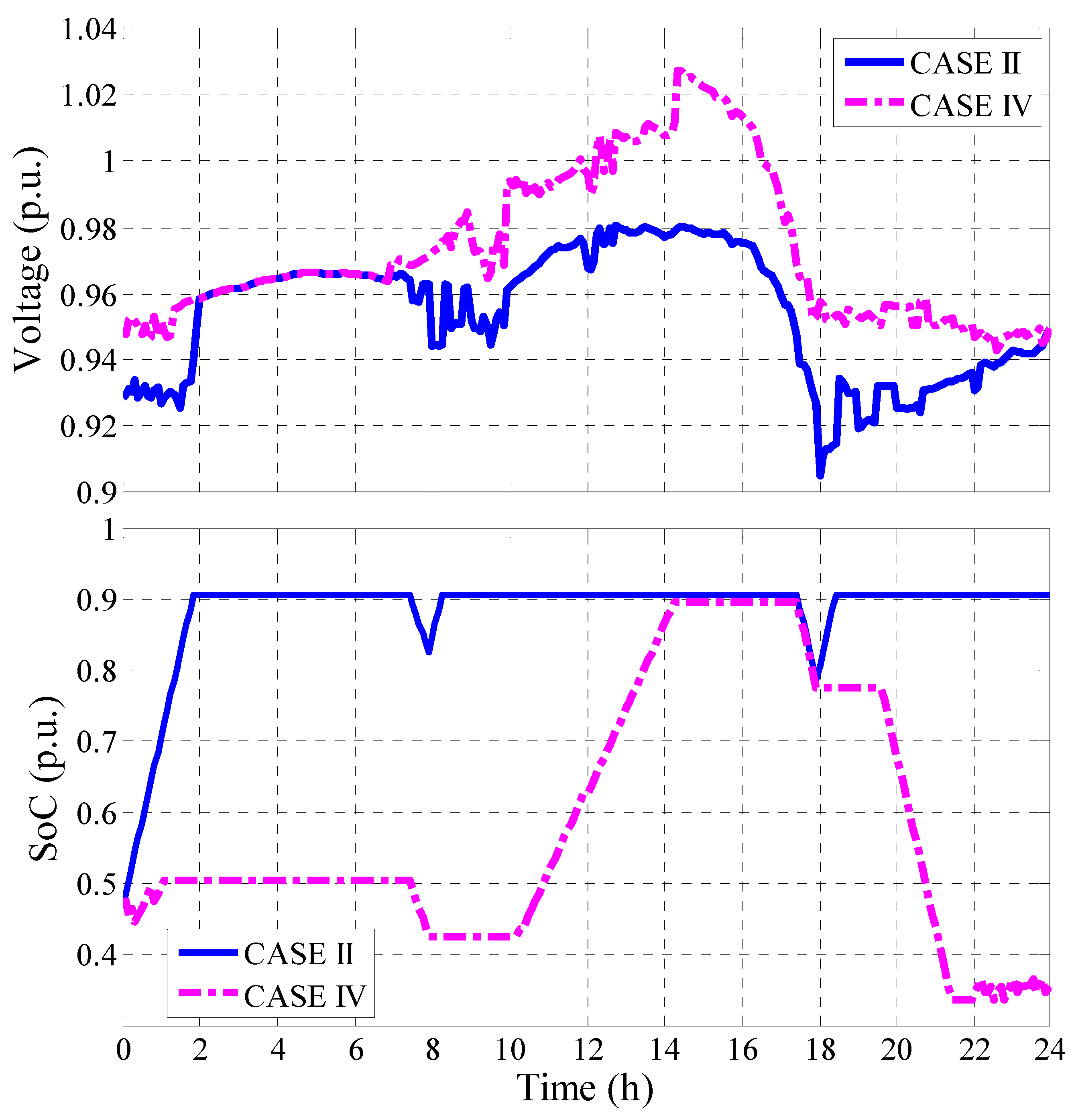
4.3. Analysis of Plug-in Electric Vehicle Impact

To show the impact of PEVs on the voltage profile at different buses, voltage profile of bus 10 in Figure 5 (bus 5 on feeder 2), is depicted in Figure 8 for CASE II and CASE IV. As mentioned earlier, bus 10 is the worst bus of the system. The role of PEVs for both negative and positive balance is demonstrated in Figure 8. In CASE II, the PEV is fully charged during the night, whereas in CASE IV the PEV charging is limited to 50%. The difference in settings causes the voltage difference between the two cases as well. PEV is on the road around 7:30 a.m. until 8:00 a.m., and it loses part of its charge. During the day time, as the solar irradiation increases, the PEV battery starts charging until around 2:00 p.m. However, after this time, although the solar power is still high, the battery reaches its maximum capacity (90%) and cannot participate in positive balance. This causes an increase in voltage. The PEV is on the road around 5:30 p.m. until 6:00 p.m. as well. As PEV becomes idle in the evening, it starts supporting the grid in CASE IV. The provided support by PEVs in this scenario is quite significant, and it clearly elevates the voltage profile of the bus. It can be seen that, despite the higher PV penetration in CASE IV compared to CASE II (32.7% higher as mentioned above), the algorithm keeps voltage deviation in the grid less than 10%.
Figure 8. Voltage profile and SoC for bus 10: CASE II and CASE IV.
Energies 09 00034 g008
Figure 9 compares the voltage profile of bus 10, and the SoC of PEV for this bus, for CASE III and CASE IV. For CASE III, the night charging is not limited, while it is limited to 50% for CASE IV. Therefore, voltage profile of bus 10 has lower values for night hours. On the other hand, when the PEV is idle during the day, the grid uses PEV storage for storing the solar production. However, since the available PEV storage is limited in CASE III compared to CASE IV, the PEV provides less grid support (positive balance) for the grid. Such scenario results in lower solar penetration, as presented in Table 2. Therefore, solar penetration is higher in CASE IV (205 panels) compared to CASE III (177 panels). Transformer power profile is presented in Figure 10 for 40 PEVs (25% penetration) in the grid. Considering the results of CASE II as the base case, it can be seen that PEV charging during the night time for CASE II occupies almost all the transformer capacity.
PV penetration provides extra power which can support the upper grid during the day. However, PV production doesn’t exist during evening time, when the grid has a significant peak in demand. Therefore, the grid is forced to absorb power from the upper grid to support its consumption. Using PEVs for grid support, the excess available energy can be stored in PEVs batteries during the daytime. The stored energy can then be used during the evening hours to respond to the peak demand of the grid. Such opportunity provides a great flexibility for the grid to not only provide some extra power to the upper grid, but the grid can also deal with its peak demand problem.
Figure 9. Voltage profile and SoC for bus 10: CASE III and CASE IV.
Energies 09 00034 g009
Figure 10. Transformer power profile for different cases.
Energies 09 00034 g010

5. Conclusions

This work focuses on the challenges and opportunities of a grid with the presence of PV panels and PEVs. The idea is to find a proper solution for the new challenges in the grid without changing the grid existing conditions, as well as benefiting from the new potentials. The focus is to utilize the PEV storage to provide maximum ancillary service. Different scenarios are evaluated to support the proposed method. Simulation results quantify the potential and effect of PEVs for the grid and the grid operator. From the results in Table 2, compared to CASE II where only positive balance is available, enabling both positive balance and negative balance increases the PV penetration by 50% with 40 PEVs in the grid (25% PEV penetration), and by 22.4% for 16 PEVs in the grid (10% PEV penetration). In addition, PV panels are optimally allocated through different grid feeders and buses to maximize the ancillary service. The results verify the capability of PEV storage in increasing the penetration of renewable energy in the grid, which leads to a more sustainable power system.

Author Contributions

Reza Ahmadi Kordkheili is the main researcher who initiated and organized research reported in the paper. He contributed to the sections on load modeling and grid modeling, EV modeling, designing intelligent algorithm, and optimization. In addition, as the first author, he is responsible for writing main parts of the paper, including paper layout and results. S. Ali Pourmousavi contributed in designing algorithms and optimization method, as well as drafting the article. Mehdi Savaghebi and Josep M. Guerrero assisted with the vehicle-to-grid application and algorithm, and contributed jointly to analysis, and the writing of this article. M. Hashem Nehrir contributed towards the optimization algorithm, and his comments on the paper draft have had a big impact on improving its quality. All authors were involved in preparing the manuscript.

Conflicts of Interest

The authors declare no conflict of interest.

Appendix A

Table A1. Parameters of genetic algorithm (GA).
ParameterPopulationNumber of GenerationStall GenerationTolerance Function
Value402001001 × 10−8
Table A2. Data of grid cables.
Bus NumberR (Ω/km)X (Ω/km)RXR (p.u.)X (p.u.)
Trafo →1 (feeder 1)0.20800.0860.08590.035553,70322,204
1 to 20.64200.08700.03990.005424,9583382
1 to 30.64200.08700.06580.008941,1285573
3 to 40.64200.08700.06420.008740.1255438
4 to 50.32100.08600.05510.014834,4679234
Trafo →6 (feeder 2)0.20800.08400.05390.021733,65713,592
6 to 70.20800.08400.01860.007511,6094688
7 to 80.20800.08400.04480.018128,02811,319
8 to 90.32100.08400.05440.014234,0068899
9 to 100.32100.08400.02580.006816,1304221
Trafo →11 (feeder 3)0.20800.08400.03470.014021,6718752
11 to 120.20800.08400.02330.009414,5605880
12 to 130.32100.08400.02610.006816,3314274
13 to 140.32100.08400.05460.014334,1068925
Trafo →15 (feeder 4)0.20800.08400.06130.024738,28515,461
15 to 160.20800.08400.02230.009013,9495633
16 to 170.20800.08400.02670.010816,7186752
17 to 180.20800.08400.01320.005382683339
Trafo →19 (feeder 5)0.20800.08600.09080.037656,77123,473
19 to 200.32100.08400.04140.010825,9016778
20 to 210.64200.08700.05450.007434,0664616
Trafo →22 (feeder 6)0.20800.08400.05900.023836,85514,884
22 to 230.20800.08400.01460.005991003675
23 to 240.38900.08300.02040.004412,7642723
24 to 250.38900.08300.03110.006619,4504150
24 to 260.52600.08300.03950.006224,6563891

References

  1. Guide for Smart Grid Interoperability of Energy Technology Operation with Electric Power System (EPS), and End-Use Applications and Loads; IEEE P2030; IEEE Standards Association: Piscataway, NJ, USA, 2011.
  2. CEN-CENELEC-ETSI Smart Grid Coordination Group-Sustainable Processes; European Committee for Electrotechnical Standardization-European Telecommunications Standards Institute (CENELEC-ETSI): Brussels, Belgium, 2012.
  3. Shafiullah, G.M.; Oo, A.M.T.; Jarvis, D.; Ali, A.B.M.S.; Wolfs, P. Potential Challenges: Integrating Renewable Energy with the Smart Grid. In Proceedings of the 20th Australasian Universities Power Engineering Conference, Christchurch, New Zealand, 5–8 December 2010; pp. 1–6.
  4. Omran, W.A.; Kazerani, M.; Salama, M.M.A. Investigation of Methods for Reduction of Power Fluctuations Generated from Large Grid-Connected Photovoltaic Systems. IEEE Trans. Energy Convers. 2011, 26, 318–327. [Google Scholar] [CrossRef]
  5. Ueda, Y.; Kurokawa, K.; Tanabe, T.; Kitamura, K.; Sugihara, H. Analysis Results of Output Power Loss Due to the Grid Voltage Rise in Grid-Connected Photovoltaic Power Generation Systems. IEEE Trans. Ind. Electron. 2008, 55, 2744–2751. [Google Scholar] [CrossRef]
  6. Tonkoski, R.; Turcotte, D.; EL-Fouly, T.H.M. Impact of High PV Penetration on Voltage Profiles in Residential Neighborhoods. IEEE Trans. Sustain. Energy 2012, 3, 518–527. [Google Scholar] [CrossRef]
  7. Hung, D.Q.; Mithulananthan, N. Multiple Distributed Generator Placement in Primary Distribution Networks for Loss Reduction. IEEE Trans. Ind. Electron. 2013, 60, 1700–1708. [Google Scholar] [CrossRef]
  8. Al-Sabounchi, A.; Gow, J.; Al-Akaidi, M. Simple Procedure for Optimal Sizing and Location of a Single Photovoltaic Generator on Radial Distribution Feeder. IET Renew. Power Gener. 2014, 8, 160–170. [Google Scholar] [CrossRef]
  9. Lin, C.H.; Hsieh, W.L.; Chen, C.S.; Hsu, C.T.; Ku, T.T. Optimization of Photovoltaic Penetration in Distribution Systems Considering Annual Duration Curve of Solar Irradiation. IEEE Trans. Power Syst. 2012, 27, 1090–1097. [Google Scholar] [CrossRef]
  10. Shaaban, M.F.; Atwa, Y.M.; El-Saadany, E.F. DG Allocation for Benefit Maximization in Distribution Networks. IEEE Trans. Power Syst. 2013, 28, 639–649. [Google Scholar] [CrossRef]
  11. Alsokhiry, F.; Lo, K.L. Distributed Generation Based on Renewable Energy Ancillary Services. In Proceedings of the 2013 Fourth International Conference on Power Engineering, Energy and Electrical Drives, Istanbul, Turkey, 13–17 May 2013; pp. 1200–1205.
  12. Kempton, W.; Tomić, J. Vehicle-to-Grid Power Implementation: From Stabilizing the Grid to Supporting Large-Scale Renewable Energy. J. Power Sources 2005, 144, 280–294. [Google Scholar] [CrossRef]
  13. Sortomme, E.; El-Sharkawi, M.A. Optimal Charging Strategies for Unidirectional Vehicle-to-Grid. IEEE Trans. Smart Grid 2011, 2, 131–138. [Google Scholar] [CrossRef]
  14. Hong, Y.-Y.; Lai, Y.-M.; Chang, Y.-R.; Lee, Y.-D.; Liu, P.-W. Optimizing Capacities of Distributed Generation and Energy Storage in a Small Autonomous Power System Considering Uncertainty in Renewables. Energies 2015, 8, 2473–2492. [Google Scholar] [CrossRef]
  15. Gao, S.; Chau, K.T.; Liu, C.; Wu, D.; Chan, C.C. Integrated Energy Management of Plug-in Electric Vehicles in Power Grid with Renewables. IEEE Trans. Veh. Technol. 2014, 63, 3019–3027. [Google Scholar] [CrossRef]
  16. Escudero-Garzas, J.J.; Garcia-Armada, A.; Seco-Granados, G. Fair Design of Plug-in Electric Vehicles Aggregator for V2G Regulation. IEEE Trans. Veh. Technol. 2012, 61, 3406–3419. [Google Scholar] [CrossRef]
  17. Rottondi, C.; Fontana, S.; Verticale, G. Enabling Privacy in Vehicle-to-Grid Interactions for Battery Recharging. Energies 2014, 7, 2780–2798. [Google Scholar] [CrossRef] [Green Version]
  18. Diaz, N.L.; Dragicevic, T.; Vasquez, J.C.; Guerrero, J.M. Intelligent Distributed Generation and Storage Units for DC Microgrids—A New Concept on Cooperative Control Without Communications Beyond Droop Control. IEEE Trans. Smart Grid 2014, 5, 2476–2485. [Google Scholar] [CrossRef]
  19. Wu, D.; Tang, F.; Dragicevic, T.; Vasquez, J.C.; Guerrero, J.M. A Control Architecture to Coordinate Renewable Energy Sources and Energy Storage Systems in Islanded Microgrids. IEEE Trans. Smart Grid 2015, 6, 1156–1166. [Google Scholar] [CrossRef]
  20. Latvakoski, J.; Mäki, K.; Ronkainen, J.; Julku, J.; Koivusaari, J. Simulation-Based Approach for Studying the Balancing of Local Smart Grids with Electric Vehicle Batteries. Systems 2015, 3, 81–108. [Google Scholar] [CrossRef]
  21. Marler, R.T.; Arora, J.S. Survey of Multi-Objective Optimization Methods for Engineering. Struct. Multidiscip. Optim. 2004, 26, 369–395. [Google Scholar] [CrossRef]
  22. Kordkheili, R.A.; Pourmousavi, S.A.; Pillai, J.R.; Hasanien, H.M.; Bak-Jensen, B.; Nehrir, M.H. Optimal Sizing and Allocation of Residential Photovoltaic Panels in a Distribution Network for Ancillary Services Application. In Proceedings of the 2014 International Conference on Optimization of Electrical and Electronic Equipment, Bran, Romania, 22–24 May 2014; pp. 681–687.
  23. Liang, H.; Zhuang, W. Stochastic Modeling and Optimization in a Microgrid: A Survey. Energies 2014, 7, 2027–2050. [Google Scholar] [CrossRef]
  24. Technical Regulation 3.2.1 for Electricity Generation Facilities with a Rated Current of 16 A per Phase or Lower; Energinet.dk: Fredericia, Denmark, 2011.
  25. Saadat, H. Power System Analysis, 2nd ed.; Mc-Graw Hill: New York, NY, USA, 2002. [Google Scholar]
  26. Pillai, J.R.; Huang, S.; Bak-Jensen, B.; Mahat, P.; Thogersen, P.; Moller, J. Integration of Solar Photovoltaics and Electric Vehicles in Residential Grids. In Proceedings of the 2013 IEEE Power and Energy Society General Meeting, Vancouver, BC, Canada, 21–25 July 2013.
  27. Thompson, M.; Infield, D.G. Impact of Widespread Photovoltaics Generation on Distribution Systems. IET Renew. Power Gener. 2007, 1, 33–40. [Google Scholar] [CrossRef]
  28. Neimane, V. On Development Planning of Electricity Distribution Networks. Ph.D. Thesis, Kungliga Tekniska högskolan (KTH), Stockholm, Sweden, 2001. [Google Scholar]
  29. Kordkheili, R.A.; Bak-Jensen, B.; Pillai, J.R.; Mahat, P. Determining Maximum Photovoltaic Penetration in a Distribution grid Considering Grid Operation Limits. In Proceedings of the 2014 IEEE PES General Meeting/Conference & Exposition, National Harbor, MD, USA, 27–31 July 2014; pp. 1–5.
  30. Alimisis, V.; Hatziargyriou, N.D. Evaluation of a Hybrid Power Plant Comprising Used EV-Batteries to Complement Wind Power. IEEE Trans. Sustain. Energy 2013, 4, 286–293. [Google Scholar] [CrossRef]
  31. Affanni, A.; Bellini, A.; Franceschini, G.; Guglielmi, P.; Tassoni, C. Battery Choice and Management for New-Generation Electric Vehicles. IEEE Trans. Ind. Electron. 2005, 52, 1343–1349. [Google Scholar] [CrossRef]
  32. Sundstrom, O.; Binding, C. Flexible Charging Optimization for Electric Vehicles Considering Distribution Grid Constraints. IEEE Trans. Smart Grid 2012, 3, 26–37. [Google Scholar] [CrossRef]

