
Prediction Performance of an Artificial Neural Network Model for the Amount of Cooling Energy Consumption in Hotel Rooms

Abstract
:1. Introduction
2. Development of a Prediction Model
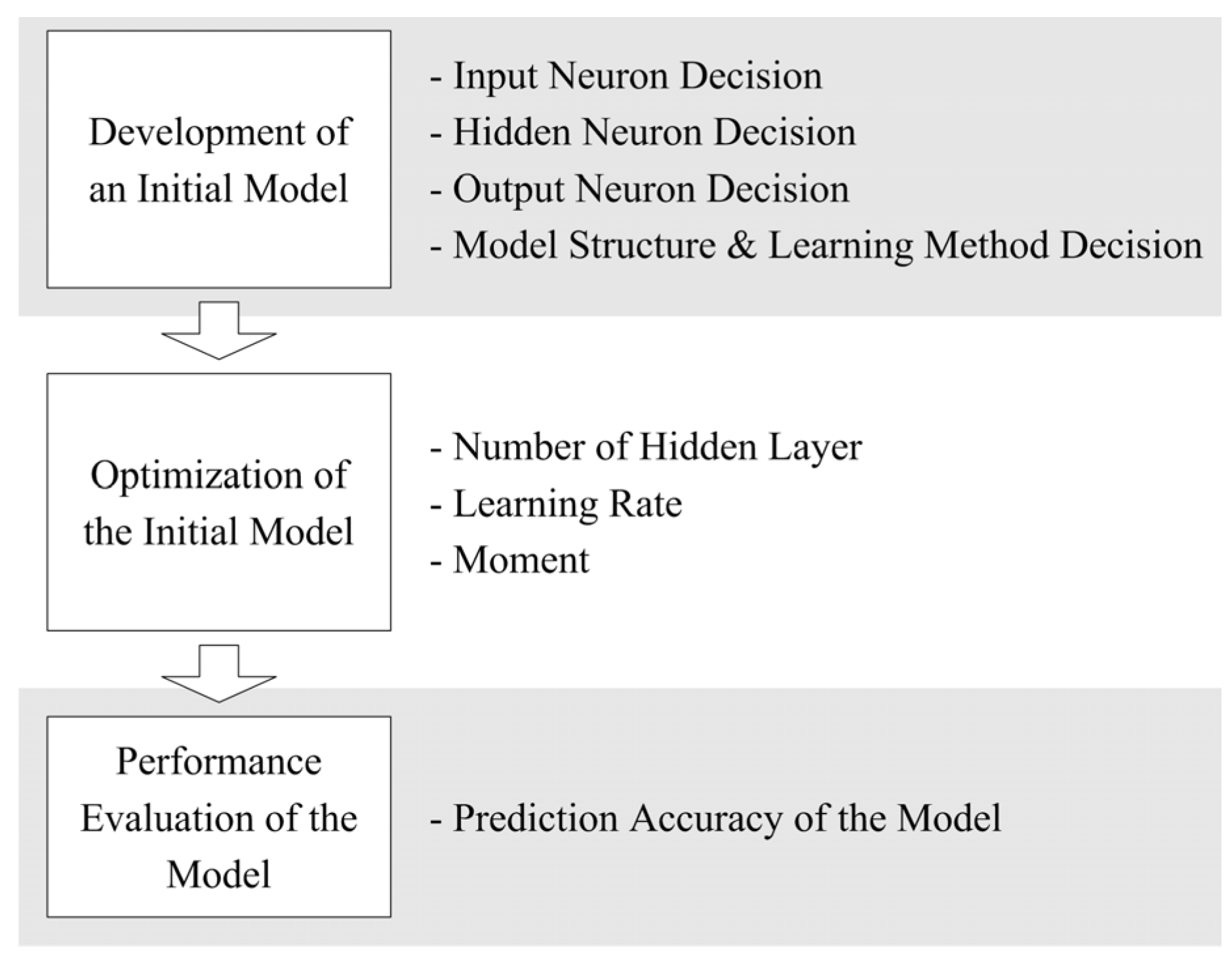
2.1. Development of the Initial Model


| Parameters | Components and values | |
|---|---|---|
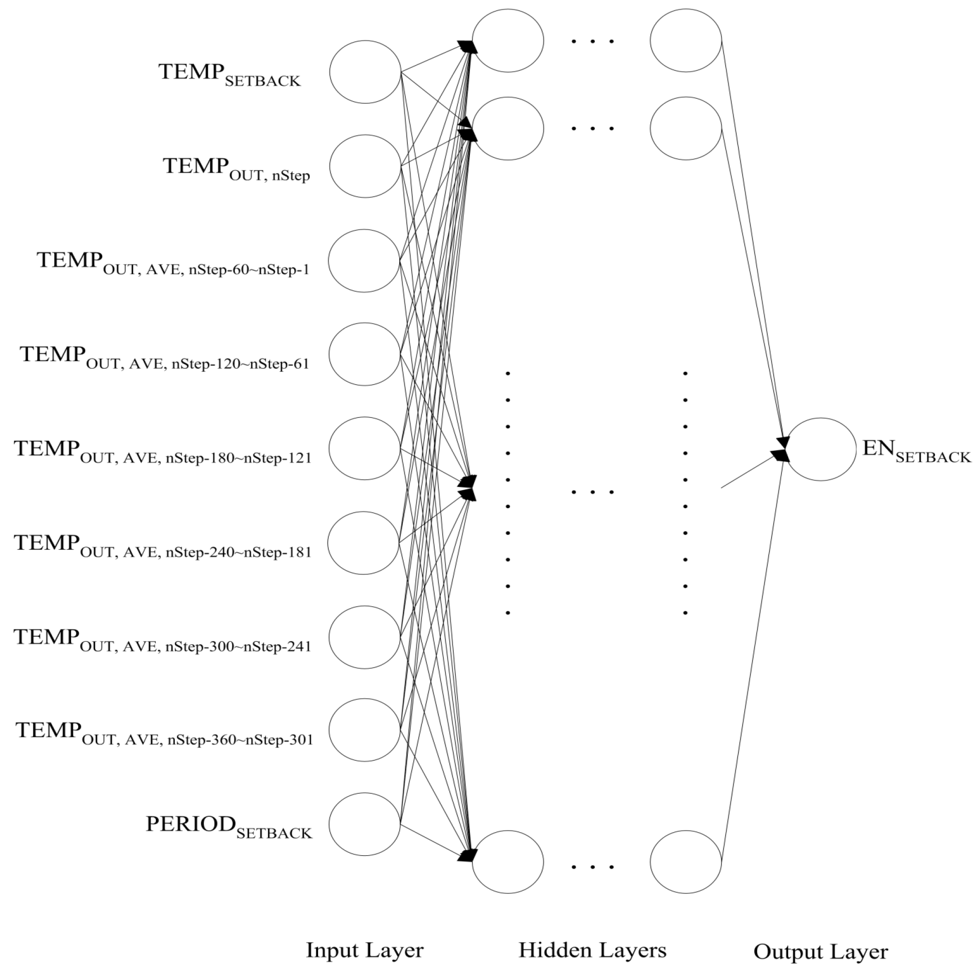
| Structure | Input layer | Number of neurons: 9 i) TEMPSETBACK ii) TEMPOUT, nStep iii) TEMPOUT, AVE, nStep-60~nStep-1 iv) TEMPOUT, AVE, nStep-120~nStep-61 v) TEMPOUT, AVE, nStep-180~nStep-121 vi) TEMPOUT, AVE, nStep-240~nStep-181 vii) TEMPOUT, AVE, nStep-300~nStep-241 viii) TEMPOUT, AVE, nStep-360~nStep-301 ix) PERIODSETBACK |
| Hidden layer | Number of neurons: 19 using Nh = 2Ni + 1 [11,33] Number of hidden Layer: 1 | |
| Output layer | Number of neuron: 1 i) ENSETBACK | |
| Transfer function | Hidden neurons | Tangent sigmoid |
| Output neurons | Pure linear | |
| Training method | Goal | 0.01 kWh (mean square error) |
| Epoch | 1,000 times | |
| Learning rate | 0.6 [34] | |
| Moment | 0.4 [34] | |
| Algorithm | Levenberg-marquardt [1,35,36,37] | |
| Number of data sets | 196 using Nd = (Nh – (Ni + No)/2)2 [12] | |
| Data management technique | Sliding-window method | |


| Components | Contents | ||
|---|---|---|---|
| Site | Location and weather data | Seoul, South Kroea (latitude: 37.56°N, longitude: 126.98°E) and TMY2 | |
| Climate conditions | Hot and humid in summer: 23.5 °C of air temperature and 72.7% of relative humidity from June to September in average Cold in winter: 1.7 °C of air temperature and 59.1% of relative humidity from November to February in average | ||
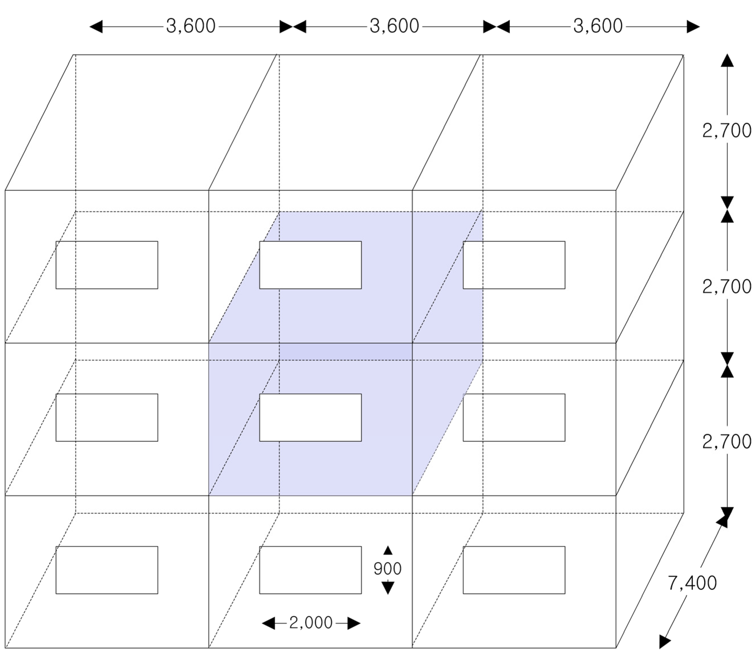
| Dimension | Module | 26.64 m2 3.6 m wide × 7.4 m deep × 2.7 m high | |
| Window | 1.8 m2 2.0 m wide × 0.9 m high | ||
| Envelope insulation [m2 K /W] [41] | Exterior walls | 2.801 | |
| Interior walls, roof and floor | 0.492 | ||
| Windows | 0.353 | ||
| Infiltration rate [41] | 0.7 ACH | ||
| Internal gain | 1 occupant with seated, light work, typing 1 computer and printer 5 W/m2 lighting fixtures | ||
| Applied system [42] | Convective cooling: 8901 kJ/hr heat removal | ||
| Components | Roles |
|---|---|
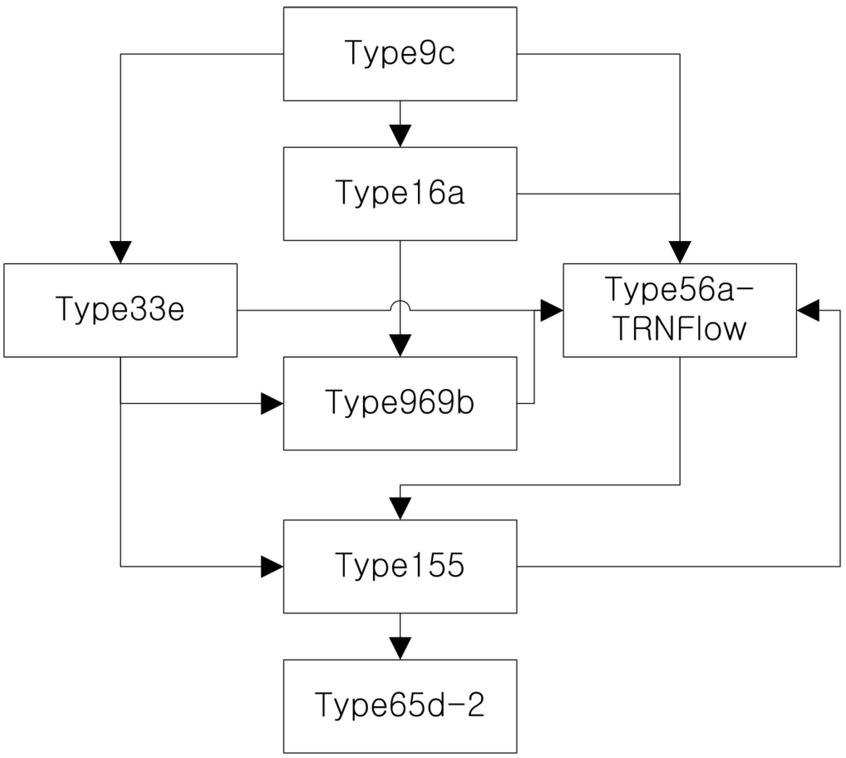
| Type9c | Reading the TMY2 weather file Transferring the weather data to the Type16a, Type33e, and Type56a-TRNFlow |
| Type16a | Calculating the amount of solar radiation on the test building surface Transferring the data to Type69b |
| Tpe69b | Calculating the sky temperature Transferring the data to the Type56a-TRNFlow |
| Type33e | Calculating the outdoor dew-point temperature Transferring the data to Type69b |
| Type56a-TRNFlow | Calculating the indoor temperature of the test building Transferring the data to Type 155 |
| Type155 | Connecting the MATBAL and ANN models Producing training data sets |
| Type65d-2 | Producing the output file |
| Data sets | 1 | 2 | 3 | 4 | 5 | |
|---|---|---|---|---|---|---|
| Input components (actual value in parenthesis, °C for TEMP and minutes for PERIOD) | TEMPSETBACK | 0.00 (23.00) | 0.00 (23.00) | 0.00 (23.00) | 0.00 (23.00) | 0.00 (23.00) |
| TEMPOUT, nStep | 0.65 (19.07) | 0.67 (20.15) | 0.66 (19.65) | 0.70 (21.78) | 0.68 (20.72) | |
| TEMPOUT, AVE, nStep-60~nStep-1 | 0.64 (18.29) | 0.65 (19.28) | 0.65 (19.10) | 0.68 (21.01) | 0.66 (19.70) | |
| TEMPOUT, AVE, nStep-120~nStep-61 | 0.64 (18.17) | 0.63 (17.54) | 0.63 (18.04) | 0.66 (19.47) | 0.63 (17.70) | |
| TEMPOUT, AVE, nStep-180~nStep-121 | 0.65 (18.89) | 0.60 (15.83) | 0.62 (16.99) | 0.63 (17.96) | 0.60 (15.73) | |
| TEMPOUT, AVE, nStep-240~nStep-181 | 0.66 (19.62) | 0.59 (15.51) | 0.61 (16.58) | 0.63 (17.90) | 0.59 (15.19) | |
| TEMPOUT, AVE, nStep-300~nStep-241 | 0.67 (20.34) | 0.60 (15.97) | 0.61 (16.54) | 0.64 (18.66) | 0.59 (15.49) | |
| TEMPOUT, AVE, nStep-360~nStep-301 | 0.68 (21.06) | 0.61 (16.45) | 0.61 (16.53) | 0.66 (19.43) | 0.60 (15.82) | |
| PERIODSETBACK | 1.00 (600) | 1.00 (600) | 1.00 (600) | 1.00 (600) | 1.00 (600) | |
| Output component, minutes (actual value in parenthesis, kWh) | ENSETBACK | 126.00 (5.19) | 192.00 (7.91) | 157.00 (6.47) | 146.00 (6.02) | 172.00 (7.09) |
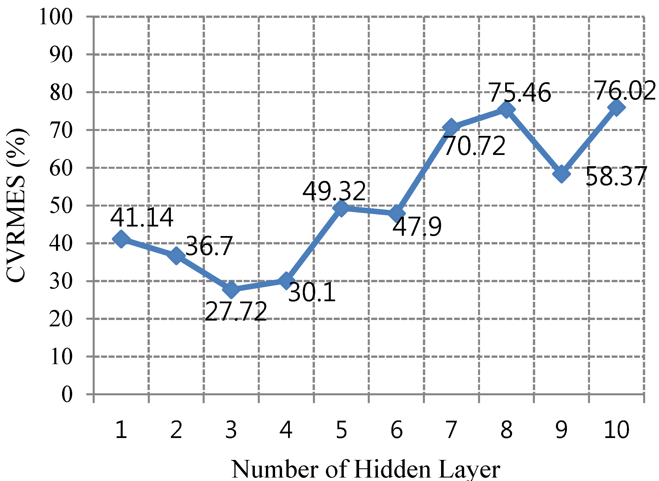
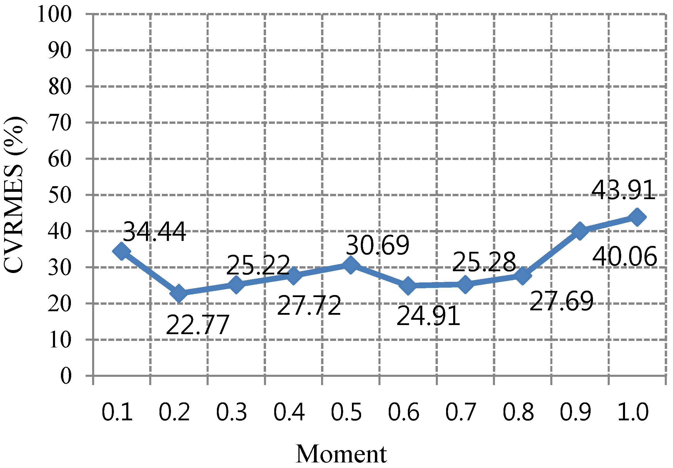
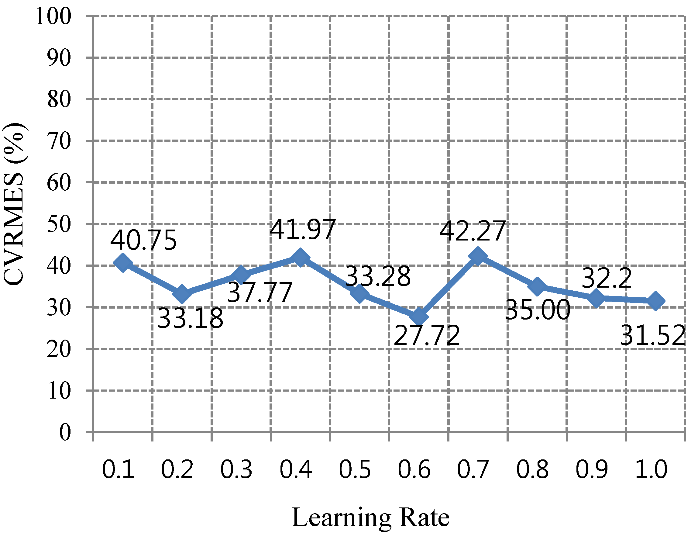
2.2. Optimization of the Initial Model
| Components to be optimized | Parametrical values to be tested | |||||||||
|---|---|---|---|---|---|---|---|---|---|---|
| Number of hidden layer | 1 | 2 | 3 | 4 | 5 | 6 | 7 | 8 | 9 | 10 |
| Learning rate | 0.1 | 0.2 | 0.3 | 0.4 | 0.5 | 0.6 | 0.7 | 0.8 | 0.9 | 1.0 |
| Moment | 0.1 | 0.2 | 0.3 | 0.4 | 0.5 | 0.6 | 0.7 | 0.8 | 0.9 | 1.0 |
2.3. Performance Evaluation of the Optimized ANN Model
3. Results Analysis
3.1. Initial Model and Optimization

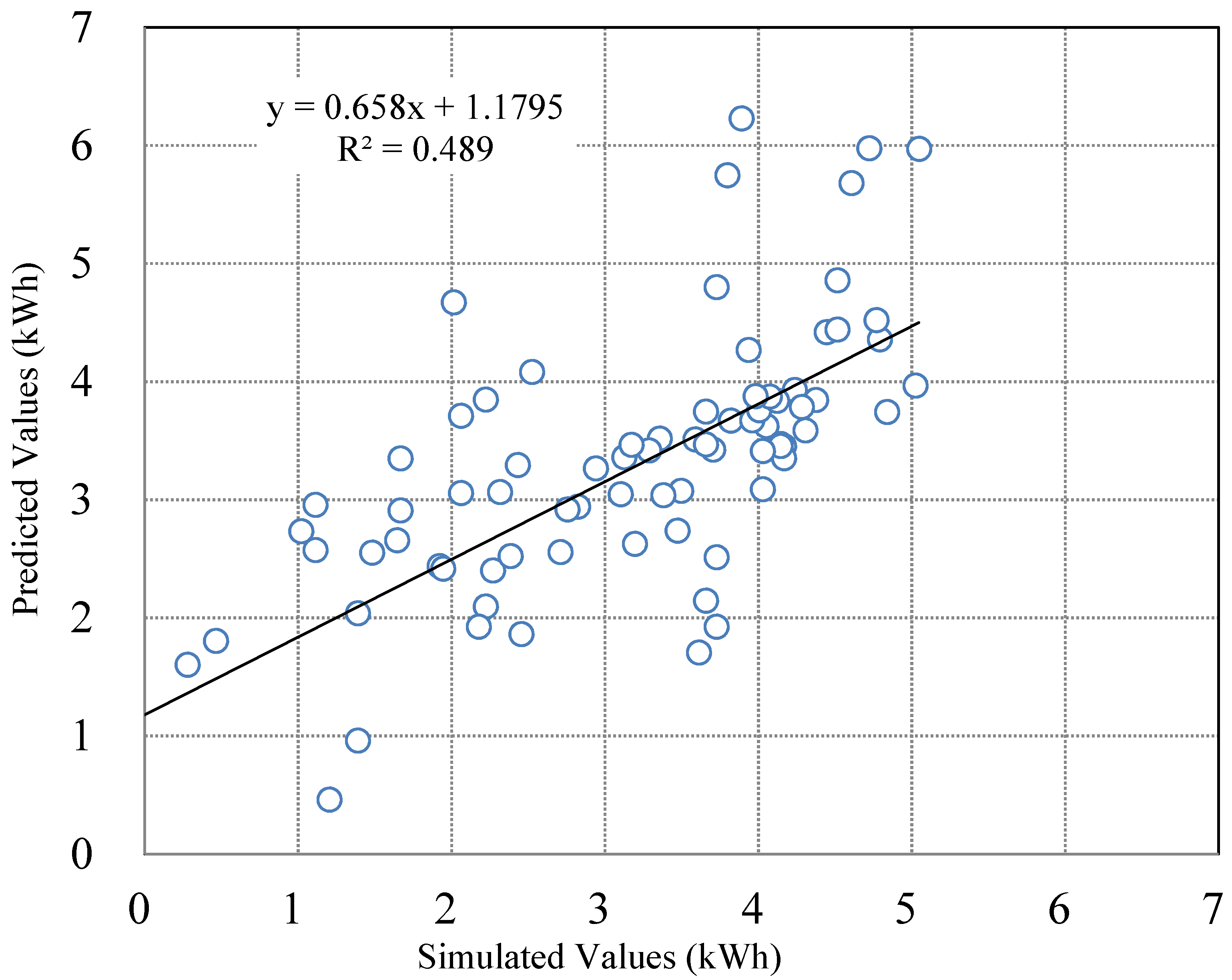
| Independent variables | Unstandardized coefficients | t | Significance. | ANOVA | |||
|---|---|---|---|---|---|---|---|
| B | Std. error | R2 | F(1, 54) | Significance. | |||
| Predicted Values | 0.658 | 0.068 | 9.677 | <0.001 | 0.489 | 93.642 | <0.001 |


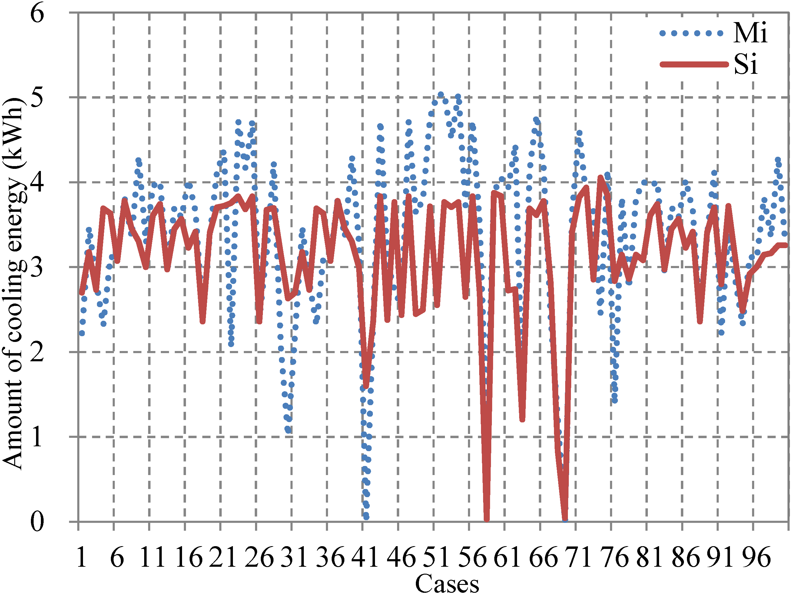
3.2. Performance of the Optimized Model

4. Conclusions
Acknowledgments
Author Contributions
Conflicts of Interest
Nomenclature:
| TEMPSETBACK | setback temperature, °C |
| TEMPOUT, nStep | outdoor air temperature in the current control cycle, °C |
| TEMPOUT, AVE, nStep-60~nStep-1 | average outdoor air temperature from nStep-60 to nStep-1, °C |
| TEMPOUT, AVE, nStep-120~nStep-61 | average outdoor air temperature from nStep-120 to nStep-61, °C |
| TEMPOUT, AVE, nStep-180~nStep-121 | average outdoor air temperature from nStep-180 to nStep-121, °C |
| TEMPOUT, AVE, nStep-240~nStep-181 | average outdoor air temperature from nStep-240 to nStep-181, °C |
| TEMPOUT, AVE, nStep-300~nStep-241 | average outdoor air temperature from nStep-300 to nStep-241, °C |
| TEMPOUT, AVE, nStep-360~nStep-301 | average outdoor air temperature from nStep-360 to nStep-301, °C |
| PERIODSETBACK | setback period during the daytime, minutes |
| ENSETBACK | predicted amount of cooling energy consumption during the setback period, kWh |
| Ni | number of neurons in the input layer |
| Nh | number of neurons in the hidden layer |
| No | number of neurons in the output layer |
| VALACT | actual value of each input variable |
| VALMIN | minimal value of each input variable |
| VALMAX | maximal value of each input variable |
| Si | value predicted by the ANN model |
| Mi | numerically simulated value |
| MAVE | average of Mi |
| n | number of cases |
References
- Moon, J.W.; Kim, J.J. ANN-based thermal control methods for residential buildings. Build. Environ. 2010, 45, 1612–1625. [Google Scholar] [CrossRef]
- Moon, J.W.; Yoon, S.H.; Kim, S. Development of an artificial neural network model based thermal control logic for double skin envelopes in winter. Build. Environ. 2013, 61, 149–159. [Google Scholar] [CrossRef]
- Shameri, M.A.; Alghoul, M.A.; Sopian, K.; Fauzi, M.; Zain, M.; Elayeb, O. Perspectives of double skin façade systems in buildings and energy saving. Renew. Sustain. Energy Rev. 2011, 15, 1468–1475. [Google Scholar] [CrossRef]
- Fallahi, A.; Haghighat, F.; Elsadi, H. Energy performance assessment of double-skin façade with thermal mass. Energy Build. 2010, 4, 1499–1509. [Google Scholar] [CrossRef]
- Moon, J.W. ANN-Based Model-Free Thermal Controls for Residential Buildings. Ph.D. Thesis, Taubman College of Architecture and Urban Planning, University of Michigan, Ann Arbor, MI, USA, 2009. [Google Scholar]
- McCulloch, W.; Pitts, W. A logical calculus of ideas immanent in nervous activity. Bull. Math. Biophys. 1943, 5, 115–133. [Google Scholar] [CrossRef]
- Moon, J.W.; Jung, S.K.; Kim, Y.; Han, S. Comparative study of artificial intelligence-based building thermal control methods—Application of fuzzy, adaptive neuro-fuzzy inference system, and artificial neural network. Appl. Therm. Eng. 2011, 31, 2422–2429. [Google Scholar] [CrossRef]
- Kalogirou, S.A.; Neocleous, C.C.; Schizas, C.N. Building heating load estimation using artificial neural networks. In Proceedings of the International Conference CLIMA 2000, Brussels, Belgium, 30 August–2 September 1997; pp. 1–8.
- Shin, K.W.; Lee, Y.S. The study on cooling load forecast of an unit building using neural networks. Int. J. Air Cond. Refrig. 2003, 11, 170–177. [Google Scholar]
- Kim, S.H.; Kim, B.S. Building load prediction using artificial neural networks in office renovation. In Proceeding of 3rd International Symposium on Architectural Interchanges in Asia, The Architectural Institute of Korea, Cheju, Korea, 23–25 February 2000; pp. 604–612.
- Datta, D.; Tassou, S.A.; Marriott, D. Application of neural networks for the prediction of the energy consumption in a supermarket. In Proceedings of the International Conference CLIMA 2000, Brussels, Belgium, 30 August–2 September 1997; pp. 98–107.
- Kalogirou, S.A.; Bojic, M. Artificial neural networks for the prediction of the energy consumption of a passive solar building. Energy 2000, 25, 479–491. [Google Scholar] [CrossRef]
- Kreider, J.F.; Wang, X.A.; Anderson, D.; Dow, J. Expert systems, neural networks and artificial intelligence applications in commercial building HVAC operations. Autom. Constr. 1992, 1, 225–238. [Google Scholar] [CrossRef]
- Aydinalp, K.M.; Ugursal, V.I. Comparison of neural network, conditional demand analysis, and engineering approaches for modeling end use energy consumption in the residential sector. Appl. Energy 2008, 85, 271–296. [Google Scholar] [CrossRef]
- Aydinalp, M.; Ugursal, V.I.; Fung, A.S. Modeling of the space and domestic hot-water heating energy-consumption in the residential sector using neural network. Appl. Energy 2004, 79, 159–178. [Google Scholar] [CrossRef]
- Platon, R.; Dehkordi, V.R.; Martel, J. Hourly prediction of a building's electricity consumption using case-based reasoning, artificial neural networks and principal component analysis. Energy Build. 2015, 92, 10–18. [Google Scholar] [CrossRef]
- Jovanović, R.Ž.; Sretenović, A.A.; Živković, B.D. Ensemble of various neural networks for prediction of heating energy consumption. Energy Build. 2015, 94, 189–199. [Google Scholar] [CrossRef]
- Yuce, B.; Li, H.; Rezgui, Y.; Petri, L.; Jayan, B.; Yang, C. Utilizing artificial neural network to predict energy consumption and thermal comfort level: An indoor swimming pool case study. Energy Build. 2014, 80, 45–56. [Google Scholar] [CrossRef]
- Pandey, S.; Hindoliya, D.A.; Mod, R. Artificial neural networks for predicting indoor temperature using roof passive cooling techniques in buildings in different climatic conditions. Appl. Soft Comput. 2012, 12, 1214–1226. [Google Scholar] [CrossRef]
- Ferreira, P.M.; Ruano, A.E.; Silva, S.; Conceição, E.Z.E. Neural networks based predictive control for thermal comfort and energy savings in public buildings. Energy Build. 2012, 55, 238–251. [Google Scholar] [CrossRef]
- Morel, N.; Bauer, M.; El-Khoury, M.; Krauss, J. Neurobat, a predictive and adaptive heating control system using artificial neural networks. Int. J. Sol. Energy 2001, 21, 161–201. [Google Scholar] [CrossRef]
- Argiriou, A.A.; Bellas-Velidis, I.; Kummert, M.; Andre, P. A neural network controller for hydronic heating systems of solar buildings. Neural Netw. 2004, 17, 424–440. [Google Scholar] [CrossRef] [PubMed]
- Argiriou, A.A.; Bellas-Velidis, I.; Balaras, C.A. Development of a neural network heating controller for solar buildings. Neural Netw. 2000, 13, 811–820. [Google Scholar] [CrossRef]
- Ben Nakhi, A.E.; Mahmoud, M.A. Energy conservation in buildings through efficient A/C control using neural networks. Appl. Energy 2002, 73, 5–23. [Google Scholar] [CrossRef]
- Abbassi, A.; Bahar, L. Application of neural network for the modeling and control of evaporative condenser cooling load. Appl. Therm. Eng. 2005, 25, 3176–3186. [Google Scholar] [CrossRef]
- Chow, T.T.; Lin, Z.; Song, C.L.; Zhang, G.Q. Applying neural network and genetic algorithm in chiller system optimization. In Proceedings of the Seventh International Building Performance Simulation Association, Rio de Janeiro, Brazil, 13–15 August 2001; pp. 1059–1065.
- Ruano, A.E.; Crispim, E.M.; Conceicao, E.Z.E.; Lucio, M.M., Jr. Prediction of building’s temperature using neural networks models. Energy Build. 2006, 38, 682–694. [Google Scholar] [CrossRef]
- Moon, J.W.; Han, S. A comparative study between thermostat/hygrometer-based conventional and artificial neural network-based predictive/adaptive thermal controls in residential buildings. J. Asian Archit. Build. Eng. 2012, 11, 169–176. [Google Scholar] [CrossRef]
- Marvuglia, A.; Messineo, A.; Nicolosi, G. Coupling a neural network temperature predictor and a fuzzy logic controller to perform thermal comfort regulation in an office building. Build. Environ. 2014, 72, 287–299. [Google Scholar] [CrossRef]
- Huang, H.; Chen, L.; Hu, E. A neural network-based multi-zone modelling approach for predictive control system design in commercial buildings. Energy Build. 2015, 97, 86–97. [Google Scholar] [CrossRef]
- Li, N.; Xia, L.; Shiming, D.; Xu, X.; Chan, M. On-line adaptive control of a direct expansion air conditioning system using artificial neural network. Appl. Therm. Eng. 2013, 53, 96–107. [Google Scholar] [CrossRef]
- Mohanraj, M.; Jayaraj, S.; Muraleedharan, C. Applications of artificial neural networks for refrigeration, air-conditioning and heat pump systems—A review. Renew. Sustain. Energy Rev. 2012, 16, 1340–1358. [Google Scholar] [CrossRef]
- Yang, J.; Rivard, H.; Zmeureanu, R. Online building energy prediction using adaptive artificial neural networks. Energy Build. 2005, 37, 1250–1259. [Google Scholar] [CrossRef]
- Moon, J.W.; Lee, J.H.; Yoon, Y.; Kim, S. Determining optimum control of double skin envelope for indoor thermal environment based on artificial neural network. Energy Build. 2014, 69, 175–183. [Google Scholar] [CrossRef]
- Moon, J.W. Performance of ANN based predictive and adaptive thermal control methods for disturbances in and around residential buildings. Build. Environ. 2011, 48, 15–26. [Google Scholar] [CrossRef]
- Baik, Y.K.; Moon, J.W. Development and performance evaluation of optimal control logics for the two position and variableheating systems in double skin façade buildings. Int. J. Korea Inst. Ecol. Archit. Environ. 2014, 14, 71–77. [Google Scholar]
- Moon, J.W. Development of integrated control methods for the heating device and surface openings based on the performance tests of the rule-based and artificial-neural-network-based control logics. Int. J. Korea Inst. Ecol. Archit. Environ. 2014, 14, 97–103. [Google Scholar] [CrossRef]
- Moon, J.W.; Han, S. Thermostat strategies impact on energy consumption in residential buildings. Energy Build. 2011, 43, 338–346. [Google Scholar] [CrossRef]
- MathWorks. MATLAB 14. Available online: http://www.mathworkgs.com/ (accessed on 5 February 2013).
- University of Wisconsin. TRNSYS16.1. Available online: http://sel.me.wisc.edu/trnsys/ (accessed on 19 December 2013).
- Design of environmental friendly houses and guidelines for performance evaluation; Ministry of Land, Transport and Maritime Affairs of Korea: Gwachon, Korea, 2009.
- Alpine. Sizing estimator for heating & cooling equipment. Available online: http://www.alpinehomeair.com/view.cfm?objID=4A176770-C3EB-4E97-AAED-C34B81D7AFED/ (accessed on 15 June 2014).
- Yang, I.H.; Yeo, M.S.; Kim, K.W. Application of artificial neural network to predict the optimal start time for heating system in building. Energy Convers. Manag. 2003, 44, 2791–2809. [Google Scholar] [CrossRef]
- Chang, J.A. Study on the Thermal Comfort and Ventilation Performance of an Underfloor Air Supply System. Ph.D. Thesis, Taubman College of Architecture and Urban Planning, University of Michigan, Ann Arbor, MI, USA, 2007. [Google Scholar]
© 2015 by the authors; licensee MDPI, Basel, Switzerland. This article is an open access article distributed under the terms and conditions of the Creative Commons Attribution license (http://creativecommons.org/licenses/by/4.0/).
Share and Cite
Moon, J.W.; Jung, S.K.; Lee, Y.O.; Choi, S. Prediction Performance of an Artificial Neural Network Model for the Amount of Cooling Energy Consumption in Hotel Rooms. Energies 2015, 8, 8226-8243. https://doi.org/10.3390/en8088226
Moon JW, Jung SK, Lee YO, Choi S. Prediction Performance of an Artificial Neural Network Model for the Amount of Cooling Energy Consumption in Hotel Rooms. Energies. 2015; 8(8):8226-8243. https://doi.org/10.3390/en8088226
Chicago/Turabian StyleMoon, Jin Woo, Sung Kwon Jung, Yong Oh Lee, and Sangsun Choi. 2015. "Prediction Performance of an Artificial Neural Network Model for the Amount of Cooling Energy Consumption in Hotel Rooms" Energies 8, no. 8: 8226-8243. https://doi.org/10.3390/en8088226
APA StyleMoon, J. W., Jung, S. K., Lee, Y. O., & Choi, S. (2015). Prediction Performance of an Artificial Neural Network Model for the Amount of Cooling Energy Consumption in Hotel Rooms. Energies, 8(8), 8226-8243. https://doi.org/10.3390/en8088226