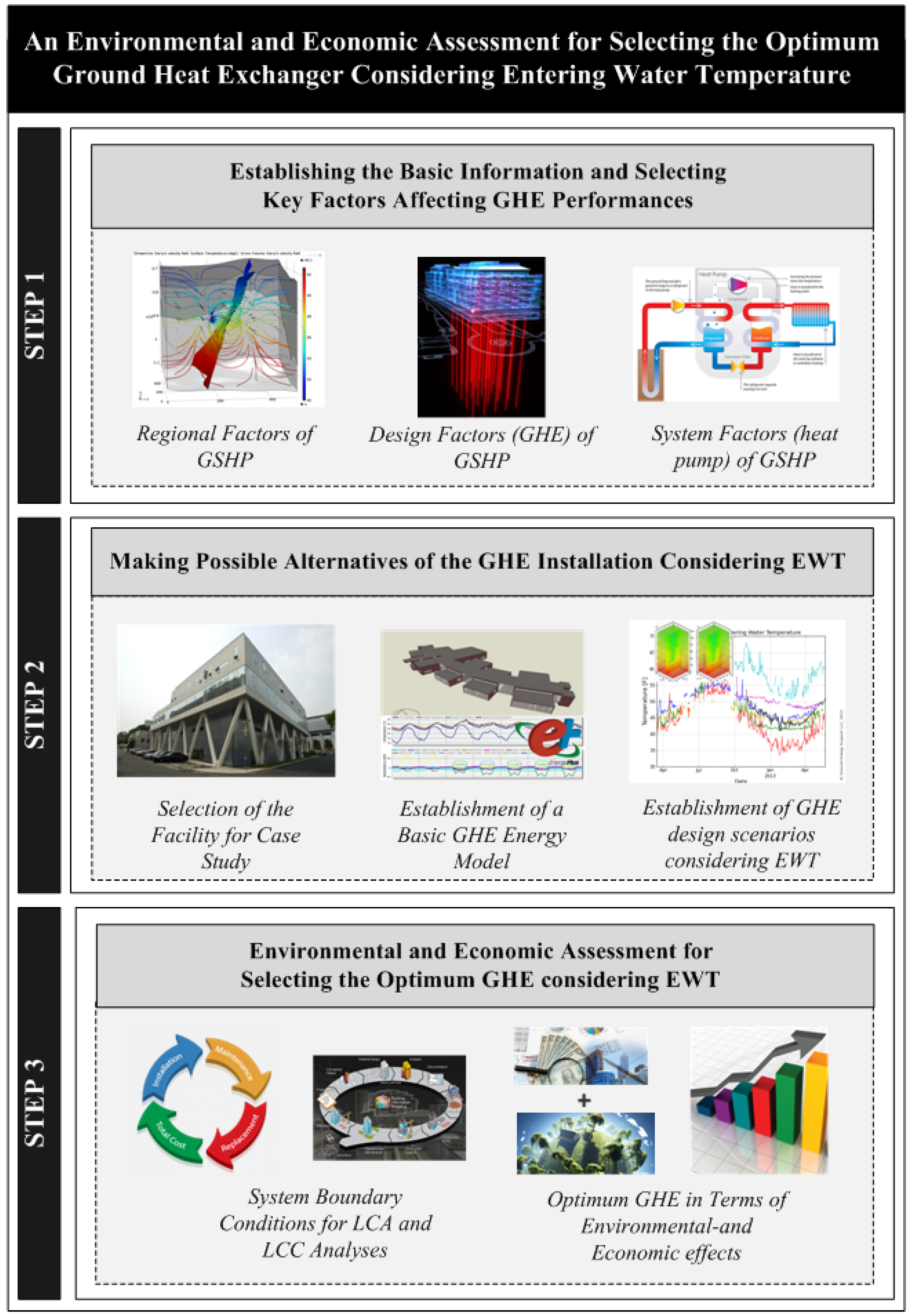
An Environmental and Economic Assessment for Selecting the Optimal Ground Heat Exchanger by Considering the Entering Water Temperature

Abstract

In order to solve environmental problems such as global warming and resource depletion in the construction industry, interest in new renewable energy (NRE) systems has increased. The ground source heat pump (GSHP) system is the most efficient system among NRE systems. However, since the initial investment cost of the GSHP is quite expensive, a feasibility study needs to be conducted from the life-cycle perspective. Meanwhile, the efficiency of GSHP depends most significantly on the entering water temperature (EWT) of the ground heat exchanger (GHE). Therefore, this study aims to assess the environmental and economic effects of the use of GHE for selecting the optimal GHE. This study was conducted in three steps: (i) establishing the basic information and selecting key factors affecting GHE performances; (ii) making possible alternatives of the GHE installation by considering EWT; and (iii) using life-cycle assessment and life-cycle cost, as well as comprehensive evaluation of the environmental and economic effects on the GHE. These techniques allow for easy and accurate determination of the optimal design of the GHE from the environmental and economic effects in the early design phase. In future research, a multi-objective decision support model for the GSHP will be developed.

1. Introduction

Excessive carbon dioxide (CO₂) emissions are currently becoming the major cause of climate change problems such as global warming and abnormal climates. Efforts to reduce CO₂ are being established across the world through the strengthening of environmental regulations such as the Kyoto Protocol. Meanwhile, South Korea imports around 97% of the total amount of energy presently used domestically. As more than 25% of these imports are used for buildings, CO₂ emissions from buildings can no longer be neglected. According to the 2013 Annual End-Use Energy Statistics, the total energy consumption of high energy consumption buildings that use 2,000 tons of equivalent (toe) each year reached 2,307,000 toe and 10,083,000 ton-CO₂, respectively. School facilities showed energy consumption of 336,000 toe and CO₂ emission of 1,397,000 ton-CO₂, which accounted for around 15% of the total amount used by buildings [1].

As the seriousness of the energy problem grows, the importance of alternative energy or new renewable energy (NRE) systems become more urgent [2,3,4,5,6,7,8,9,10,11,12,13,14]. In particular, a ground source heat pump (GSHP) system is a highly efficient NRE system for heating and cooling the building [15,16,17,18]. This system relies on a relatively constant ground temperature and can transfer the earth’s heat into a building during the winter, and transfer heat out of the building during the summer [19,20,21,22,23,24,25]. A typical GSHP system consists of a ground heat exchanger (GHE) to collect/reject heat to the ground heat pump to heat/cool the building, and pump(s) to circulate a thermal fluid between the heat pumps and the GHE [26,27,28,29,30].

There have been various studies on the environmental and economic effects of GSHP systems in a building from the following three perspectives: (i) the environmental effects of the GSHP systems were analyzed under various conditions; (ii) the economic effects of the GSHP systems in a building were analyzed; and (iii) the environmental and economic effects of GSHP systems were analyzed at the same time.

First, various studies have focused on the environmental effects of the GSHP system in a building [31,32,33,34,35]. Genchi et al. [36] assessed CO₂ payback of a GSHP system in Shinjuku, Tokyo, Japan that consumed a large amount of electric energy. The total CO₂ emissions from the installation and operation of GSHP system were estimated to be 67,701 and 33,935 tons respectively. That means the GSHP system would result in a reduction of 54% of the CO₂ emissions (39,519 ton-CO₂) compared with air source heat pumps (ASHP). If an ASHP system installed within an area of 1 km² in this region is replaced with a GSHP system, CO₂ payback-time is estimated at 1.7 years. Blum et al. [37] conducted an analysis of unit-area CO₂ savings from a GSHP system. Its scope was limited to 1105 installed GSHP systems. Compared with conventional heating systems, the minimum average total annual CO₂ savings of all installed GSHP systems is up to 2000 tons/year due to the subsidy program which promoted GSHP systems for private one-family, two-family, and terraced houses for which the heating demand is less than 17 kW in Baden-Wurttemberg, Germany. The additional CO₂ emissions are primarily associated with the affluent suburbs of the most densely populated area in the region. Saner et al. [38] conducted not only an analysis of CO₂ and energy, but also life-cycle assessment (LCA) of overall environmental damages in terms of resource depletion, human health and ecosystem quality. The analysis result showed that, although a GSHP system normally contributes to the reduction of CO₂ emissions, the GSHP system can cause water pollution.

Second, the economic effects of the GSHP system were analyzed under various conditions [39,40,41,42,43,44]. Zhu et al. [45] analyzed the economic effect of a GSHP system including life-cycle cost analysis. Life-cycle cost analysis is based on the Monte Carlo simulation. A GSHP system installed in Pensacola, U.S. was selected as a case. According to the analysis results, the effectiveness was highest when the subsidy for initial investment cost and operation cost was provided, compared with a conventional single-zone split system using heat pumps. However, where an incentive system did not exist, the feedback period was analyzed as more than 15 years. Sekine et al. [46] introduced a cast-in-place concrete pile (energy pile) method to reduce the high initial investment cost, and to improve the efficiency of the GSHP system. According to the analysis result, this system gained a competitive advantage with US$0.79/W, compared with US$3/W of the conventional system.

Third, the environmental and economic effects of GSHP systems were analyzed at same time [47,48,49]. Nagano et al. [47] developed a tool to analyze GSHP system performances, life-cycle cost (LCC) and life-cycle CO₂ (LCCO₂).They conducted a comparative evaluation of residential buildings in Sapporo, Japan using thermal response tests. For the case that the building energy loads during the winter are satisfied, they also compared the facility systems of other heat sources and their consumptions and conducted a cost analysis accordingly. Results of the calculations showed that the LCCO₂ of the GSHP system is 2038 kg-CO₂/year which is less than half compared to conventional oil boiler systems. Also, the GSHP system can reduce LCC by 50,000–90,000 Japanese yen/year. Self et al. [49] compared GSHP systems with facility systems of other heat sources in terms of LCC and LCCO₂. According to the analysis result, the GSHP system was by far lower in CO₂ emissions than other heat source systems.

In summary, there are several limitations in the previous studies: (i) most previous studies focused only on CO₂ emissions of a GSHP system; (ii) there are no previous studies focusing on the comparison analysis of the environmental and economic assessments of different entering water temperatures (EWT) of a ground heat exchanger (GHE); and (iii) there are no previous studies on the optimal GHE design alternative in terms of integrated environmental and economic assessment. This study aimed to solve these limitations.

To address these challenges, this study defined the research scope as follows: (i) the scope of environmental impact assessment was defined by life-cycle stages (including material manufacturing, use and maintenance); (ii) the scope of environmental impact categories were placed into six categories (including resource depletion potential (RDP), global warming potential (GWP), ozone layer depletion potential (ODP), acidification potential (AP), eutrophication potential (EP), and photochemical oxidation potential (POCP)); and (iii) the scope of analysis focused on GHE. Based on the defined research scope, this study aims to assess the environmental and economic effects of the use of GHE for selecting the optimal GHE. This study was conducted in three steps: (i) Establishing the basic information and selecting key factors affecting GHE performances; (ii) Creating possible alternatives for GHE installation while considering EWT; (iii) Using life-cycle assessment and life-cycle cost, as well as comprehensive evaluation of the environmental and economic effects on the GHE (refer to Figure 1).

Figure 1. Framework of the research.

Figure 1. Framework of the research.

2. Establishing the Basic Information and Selecting Key Factors Affecting Ground Heat Exchanger (GHE) Performances

Prior to designing the GSHP system, the basic information for the GSHP system installation needs to be established. The study defines the region, facility type, and power supply system type where the system is to be implemented. Furthermore, the study selects key factors affecting GSHP system performances. The study establishes the information of regional factors, design factors (GHE), and system factors (heat pump) linked with the facility to design the optimal alternative.

2.1. Regional Factors of a Ground Source Heat Pump (GSHP) System

Ground thermal conductivity, ground heat capacity and ground temperature are considered regional factors. These factors affect GSHP system performances, and the value varies depending on regions. In addition, as borehole drilling costs incurred in construction are different according to the types of soil, these factors should be investigated prior to GSHP system installation.

2.2. Design Factors of GHE for a GSHP System

GHE is largely assessed by the characteristics of the borehole, such as the number and arrangement of boreholes, borehole spacing, grout conductivity, U-tube type and size, EWT, etc. and accounts for a large proportion of cost in the initial investment of GSHP system. Each component affects the GSHP system performances individually and decides GHE performances through interaction. The details of each factor are as follows (refer to Figure 2 and Table 1):

•

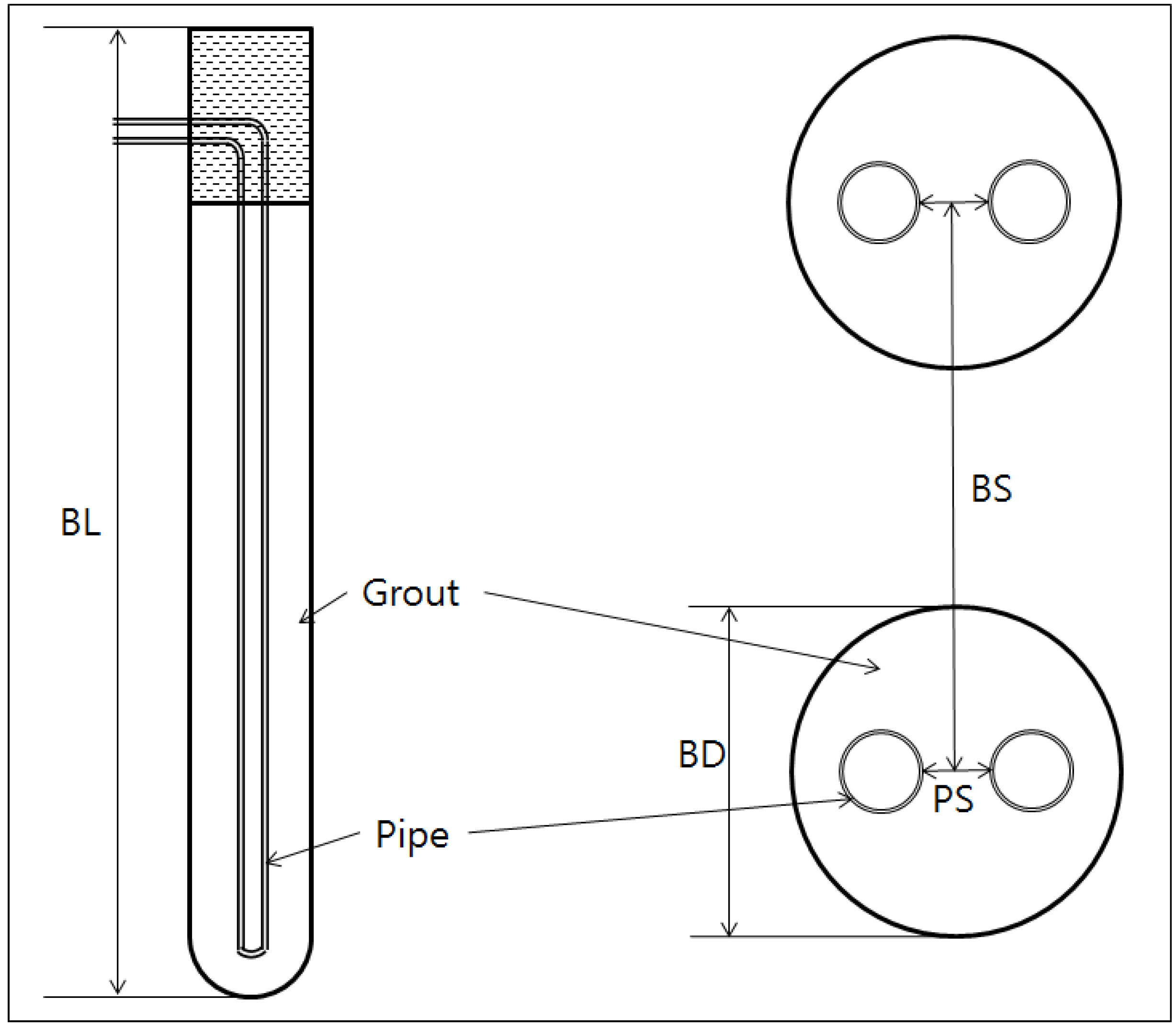
Borehole length (BL): Borehole length usually affects largely the performances and cost of GHE, and, accordingly, multi-studies are being conducted on the design of optimal length. The optimal length is decided by all the factors affecting GHE such as underground environment, GHE components and G-function.

•

Number of boreholes and arrangement: The number and arrangement of boreholes is a factor that can affect the total length of the borehole and accounts for a significant portion of the cost. Besides, as the distribution of temperature transferred to underground varies according to a type of arrangement such as L-, U- and rectangle types, this factor affects the performances of boreholes.

•

Borehole spacing (BS): As heat capacity differs according to the type of ground, optimal spacing should be designed to prevent a reduction in GHE performances caused by intersection of the scopes of ground-source heats emitted and absorbed by each borehole.

•

Borehole diameter (BD): Borehole diameter is designed in consideration of the U-pipe through which fluid flows and the volume of grout that fills a borehole. As borehole thermal resistance is higher with an increase in the volume of grout, the performance decreases. If its volume is too small, the inner components protected by grout can be impaired. Thus, it is necessary to make proper thickness.

•

U-pipe spacing (PS), pipe size and pipe type: It is necessary to combine these factors to meet temperature load in consideration of the speed of fluid that flows inside a pipe and its related heat transfer capacity. These factors, which are related to the flowing fluid the pipe directly touches, require a strength and durability above a certain level.

•

Grout conductivity: Grout conductivity is an element that constitutes a borehole. The higher its thermal conductivity, the lower the overall borehole resistance.

•

Fluid type, flow rate: Fluid type and flow rate are variables of heat transfer that occur while fluid flows in a pipe. The usual mix with other material keeps fluid from freezing.

Table 1. Overview of key factor.

Category	Key Factor (Unit)	References
Regional Factor	Ground temperature (°C), Soil type, Ground thermal conductivity (W/mK), Ground heat capacity (kJ/K·m3)	[50,51,52,53]
Ground Heat Exchanger	Borehole length (BL) (m), Borehole spacing (BS) (m), Borehole diameter (BD) (mm), U-pipe spacing (PS) (mm), Number of boreholes: arrangement, Grout conductivity (W/mK), Borehole thermal resistance (K/(W/m)), Pipe type, Pipe size, Fluid type, Flow rate (L/s), Entering water temperature (°C)	[54,55,56,57,58,59,60,61,62]
Heat Pump	Capacity (kW), Power input (kW), Heat of rejection (kW), Heat of extraction (kW), Coefficient of performance, Energy efficient rating, Entering water temperature (°C)	[27,63,64,65]

Table 1. Overview of key factor.

Category	Key Factor (Unit)	References
Regional Factor	Ground temperature (°C), Soil type, Ground thermal conductivity (W/mK), Ground heat capacity (kJ/K·m3)	[50,51,52,53]
Ground Heat Exchanger	Borehole length (BL) (m), Borehole spacing (BS) (m), Borehole diameter (BD) (mm), U-pipe spacing (PS) (mm), Number of boreholes: arrangement, Grout conductivity (W/mK), Borehole thermal resistance (K/(W/m)), Pipe type, Pipe size, Fluid type, Flow rate (L/s), Entering water temperature (°C)	[54,55,56,57,58,59,60,61,62]
Heat Pump	Capacity (kW), Power input (kW), Heat of rejection (kW), Heat of extraction (kW), Coefficient of performance, Energy efficient rating, Entering water temperature (°C)	[27,63,64,65]

Figure 2. Components of Ground Source Heat Pump (GSHP) system.

Figure 2. Components of Ground Source Heat Pump (GSHP) system.

•

Borehole thermal resistance: Borehole thermal resistance, which is the thermal resistance of the overall borehole determined by a mix of the above factors, affects the design of a borehole.

•

Entering water temperature (EWT): EWT, which is an indicator that can evaluate the final performance by a mix of each key factor, is the GHE outlet temperature that meets the energy demand of the building [66]. To calculate the EWT, Equation (1) was used [67]. EWT is designed to provide water at a high temperature in the case of heating, and at a low temperature in the case of cooling, which can minimize the load of a heat pump. Hence, the design process of the GHE will be a core factor in the design of the overall GSHP system.

$$EWT=T_g+\frac{q_i}{2m{c}_p}+\frac{Q_i{R}_b}{H}+\frac{1}{2\pi L}{\displaystyle \sum _{i=1}^N\left(Q_i-Q_{i-1}\right)g\left\{\frac{\left(t_i-t_{i-1}\right)}{t_s},\frac{r_b}{H}\right\}}$$

(1)

where, EWT is GHE outlet temperature, T_g is ground temperature, q is the net heat rejection rate, i is the index to denote the end of a time step, m is mass flow rate, C_p is specific heat of the water, Q_i is step heat rejection pulse, R_b is borehole thermal resistance, L is borehole length, H is borehole depth, t is time, t_s is time scale, r_b is borehole radius, k is ground thermal conductivity.

In this case, the total length of a borehole can be calculated by taking into account the energy and EWT necessary for the cooling and heating of the building (refer to (Equations (2) and (3))) [67].

$$L_C=\frac{\left(Capacit{y}_{Cooling}\right)\left(\frac{CO{P}_C-1}{CO{P}_C}\right)\left(R_p+R_s\cdot RunFractio{n}_h\right)}{EW{T}_{Max}-T_{g.Max.Annual}}$$

(2)

$$L_H=\frac{\left(Capacit{y}_{ Heating}\right)\left(\frac{CO{P}_H-1}{CO{P}_H}\right)\left(R_p+R_s\cdot RunFractio{n}_h\right)}{T_{g.\min .Annual}-EW{T}_{\min }}$$

(3)

where, Lc is required bore length for cooling, L_h is required bore length for heating, Capacity is capacity of ground source heat pump, COP is coefficients of performance of ground source heat pump, Rp is thermal resistance of pipe, Rs is thermal resistance of soil, RunFraction_h is runtime of heat pump, EWT is the heat pump entering liquid temperature

2.3. System Factors (Heat Pump) of GSHP System

A heat pump is directly linked to GHE; therefore, the heating and cooling loads of a target facility should be first identified. In this case, a design of heat pump can be conducted by taking into account hourly load, average daily load or average monthly load. Meanwhile, the EWT, which is the temperature of water entering from the GHE, has a considerable effect on the efficiency of a heat pump. Thus, a proper heat pump should be designed in conjunction with EWT and the energy demand of the building.

3. Creating Possible Alternatives for the GHE Installation by Considering Entering Water Temperature (EWT)

3.1. Selection of a Facility for Case Study

To conduct an environmental- and economic-effect assessment for the GHE in this study, a facility that has actually applied the GSHP system was selected as a case study. The following criteria were applied to selection:

•

According to the 2013 Annual End-Use Energy Statistics, the total energy and CO₂ emissions from high energy consumption buildings that use 2000 toe per year reached 2,307,000 toe and 10,083,000 ton-CO₂, respectively. The energy used by the schools among them reached 336,000 toe with CO₂ emissions of 1,397,000 ton-CO₂, which accounted for around 15% of the total amount used by buildings [1].

•

The GSHP system among an NRE system can be installed underground and designed around the systematic characteristics. Accordingly, the region with the lowest high building density should be selected.

•

A building that fully uses an air cooling and heating GSHP system was selected to calculate the environmental and economic effects of a GSHP system according to GHE scenarios.

Based on the above criteria, the “Y” university gym facility located in Seoul, South Korea was selected. “Y” university gym facility introduced a 422 kW GSHP system (installation capacity: 204 kW for cooling; and 218 kW for heating) in December 2012 and has replaced 100% of the annual heating and cooling energy consumption with the GSHP system. Table 2 provides data about the gym of “Y” university with regard to its characteristics and energy consumption.

Table 2. Overview of Target facility.

Category	University Facilities
Year established	2012
Location	Seoul
Building type	Educational facility
Electricity system	On-grid
Heating system	Individual heating
Progressive tax	No
Floor space of gym	1197.54 m2
Major energy service	Ground source heat pump (GSHP)
Installation of capacity	Cooling: 204 kW/Heating: 218 kW
Borehole	Length: 143 m/hole: 22 EA

Table 2. Overview of Target facility.

Category	University Facilities
Year established	2012
Location	Seoul
Building type	Educational facility
Electricity system	On-grid
Heating system	Individual heating
Progressive tax	No
Floor space of gym	1197.54 m2
Major energy service	Ground source heat pump (GSHP)
Installation of capacity	Cooling: 204 kW/Heating: 218 kW
Borehole	Length: 143 m/hole: 22 EA

3.2. Establishment of a Basic GHE Energy Model

To analyze the effect of the GSHP system on the target building, a basic energy model that reflects the current energy consumption pattern should be established. Toward this end, this study used the energy simulation software program: (i) GLHEpro which was developed by the International Ground Source Heat Pump Association (IGSHPA) in the U.S. [68]; (ii) EnergyPlus which was developed by the U.S. Department of Energy [69]. GLHEpro uses an incremental search method to change the borehole depth and then runs a simulation. The max and min EWT results are compared with the desired values, iterating until it finds a solution that matches EWT requirements. EnergyPlus was developed to be available at any stage of the design process. In this study, “Y” university gym facility has replaced 100% of the annual heating and cooling energy consumption with the GSHP system. As a result, electric energy is consumed only by a heat pump that connects GHE to the “Y” university gym facility. Therefore, in this study, a basic energy model should be established for electricity energy consumption of the heat pump.

To verify the feasibility of the energy simulation results, the coefficient of variation of the root mean square error (CV(RMSE)) wasused (Equation (4)). As shown in Figure 3, the CV(RMSE) values were 19.26% within the tolerance limits (25%) [7]. Thus, it was determined that the basic model was feasible.

$$\text{CV(RMSE)}=\frac{\sqrt{\frac{{\displaystyle \sum _{\text{i}=\text{1}}^{\text{n}}{{\text{(y}}_{\text{estimate\_usage,i}}-{\text{y}}_{\text{actual\_usage,i}}\text{)}}^{\text{2}}}}{\text{n}-\text{1}}}}{{\overline{\text{y}}}_{\text{actual\_usage}}}\times \text{100}$$

(4)

where, y_{estimate_usage,i} is electricity consumption of each month (simulation-based data), y_{actual_usage,i} is electricity consumption of each month (actual data), y_{actual_usage} is average of actual electricity consumption for 1 year, n is the number of data (months).

Figure 3. (CV)RMSE: electricity consumption of heat pump (“Y”university gym facility).

Figure 3. (CV)RMSE: electricity consumption of heat pump (“Y”university gym facility).

3.3. Establishment of GHE Design Scenarios Considering EWT

In Section 2, this study established the basic information and selecting key factors affecting GHE performances. In this case, GHE is a system that provides heat to the heat pump in the building or recovers heat through direct heat exchange from heat sources. GHE should be designed to satisfy the energy demand of the building and comprehensively consider the effects of key factors in order to create an optimal scenario in terms of environmental and cost effectiveness.

In order to design a GSHP system that can satisfy the energy demand of the target facility, scenarios for GHE were created in a condition of the existing facility (i.e., heat pumps and land). As mentioned above, GHE is designed based on EWT and the characteristics of boreholes. The number of GHE scenarios available in a situation when EWT fluctuates, increases considerably with by taking into account the energy demand of the target facility, the EWT and the characteristics of boreholes (refer to Table 3,

Table A1. Scenarios (length of borehole) of GHE considering EWT (30 °C) and characteristics of borehole.

Maximum Entering Water Temperature: 30 °C, Minimum Entering Water Temperature: 5 °C
Number of Boreholes: Arrangement (U)	Borehole Spacing	Grout Conductivity (W/mK)	U-Tube Type and Size				U-Tube Type and Size				U-Tube Type and Size
			PN10, DN25				PN10, DN32				PN10, DN40
			Borehole Diameter				Borehole Diameter				Borehole Diameter
			125 mm		150 mm		125 mm		150 mm		125 mm		150 mm
			U-Pipe Spacing				U-Pipe Spacing				U-Pipe Spacing
			3 mm	20 mm	3 mm	20 mm	3 mm	20 mm	3 mm	20 mm	3 mm	20 mm	3 mm	20 mm
22 (EA): 8 × 8	4 m	1 W/mK	157.4	142.4	159.3	145.8	134.1	123.0	135.7	126.3	114.7	105.7	116.4	108.8
		1.4 W/mK	136.5	125.1	137.1	126.9	119.1	109.7	119.7	111.3	104.2	96.9	104.8	98.2
		1.8 W/mK	124.3	113.9	124.3	114.6	109.8	101.5	109.6	102.1	97.9	91.8	97.5	92.2
	5 m	1 W/mK	156.1	141.4	157.9	144.7	133.2	121.9	134.8	125.1	113.5	104.3	115.3	107.5
		1.4 W/mK	135.6	123.9	136.2	125.8	117.9	108.5	118.5	110.1	102.9	95.7	103.4	97.0
		1.8 W/mK	123.2	112.7	123.1	113.4	108.5	100.2	108.4	100.8	96.6	90.6	96.3	91.0
	6 m	1 W/mK	155.4	140.7	157.3	144.0	132.4	120.8	134.0	124.2	112.7	103.8	114.4	106.9
		1.4 W/mK	134.9	123.0	136.5	124.8	117.1	107.8	117.7	109.4	102.3	95.3	102.9	96.6
		1.8 W/mK	122.3	111.9	122.2	112.7	107.9	99.8	107.7	100.3	96.2	90.1	95.9	90.4

,

Table A2. Scenarios (length of borehole) of GHE considering EWT (27 °C) and characteristics of borehole.

Maximum Entering Water Temperature: 23 °C, Minimum Entering Water Temperature: 5 °C
Number of Boreholes: Arrangement (U)	Borehole Spacing	Grout Conductivity (W/mK)	U-Tube Type and Size				U-Tube Type and Size				U-Tube Type and Size
			PN10, DN25				PN10, DN32				PN10, DN40
			Borehole Diameter				Borehole Diameter				Borehole Diameter
			125 mm		150 mm		125 mm		150 mm		125 mm		150 mm
			U-Pipe Spacing				U-Pipe Spacing				U-Pipe Spacing
			3 mm	20 mm	3 mm	20 mm	3 mm	20 mm	3 mm	20 mm	3 mm	20 mm	3 mm	20 mm
22 (EA): 8 × 8	4 m	1 W/mK	186.5	169.1	188.5	173.1	158.4	144.6	160.7	148.5	135.7	122.4	133.7	125.8
		1.4 W/mK	161.8	147.0	162.7	149.3	140.3	130.4	141.0	132.2	124.1	112.9	121.5	114.4
		1.8 W/mK	146.1	134.9	146.0	135.7	130.5	120.8	130.3	121.5	114.0	107.0	113.5	107.4
	5 m	1 W/mK	185.0	167.5	187.2	171.5	156.8	143.3	159.0	147.1	132.0	122.1	133.6	125.6
		1.4 W/mK	160.0	145.7	161.0	147.9	139.1	129.1	139.8	131.0	120.5	112.3	121.1	113.9
		1.8 W/mK	144.8	133.8	144.8	134.5	129.2	119.4	129.0	120.0	113.4	106.3	113.0	106.7
	6 m	1 W/mK	184.1	166.9	186.3	170.8	156.0	142.5	158.2	146.3	131.9	121.9	133.6	125.3
		1.4 W/mK	159.3	144.9	160.0	147.1	138.3	128.0	139.0	129.9	120.1	111.9	120.8	113.5
		1.8 W/mK	144.1	132.9	144.0	133.7	128.0	118.3	127.9	118.9	113.0	105.9	112.6	107.0

,

Table A3. Scenarios (length of borehole) of GHE considering EWT (25 °C) and characteristics of borehole.

Maximum Entering Water Temperature: 23 °C, Minimum Entering Water Temperature: 5 °C
Number of Boreholes: Arrangement (U)	Borehole Spacing	Grout Conductivity (W/mK)	U-Tube Type and Size				U-Tube Type and Size				U-Tube Type and Size
			PN10, DN25				PN10, DN32				PN10, DN40
			Borehole Diameter				Borehole Diameter				Borehole Diameter
			125 mm		150 mm		125 mm		150 mm		125 mm		150 mm
			U-Pipe Spacing				U-Pipe Spacing				U-Pipe Spacing
			3 mm	20 mm	3 mm	20 mm	3 mm	20 mm	3 mm	20 mm	3 mm	20 mm	3 mm	20 mm
22 (EA): 8 × 8	4 m	1 W/mK	212.6	192.9	215.4	197.0	181.5	166.3	184.1	170.4	155.1	142.6	157.5	146.8
		1.4 W/mK	185.2	168.8	186.1	171.3	161.3	148.1	162.1	150.3	140.8	132.2	141.5	133.8
		1.8 W/mK	168.0	154.0	168.0	155.0	148.1	137.7	147.9	138.3	133.4	125.1	132.9	125.6
	5 m	1 W/mK	211.2	191.5	213.8	195.7	179.8	164.4	182.2	168.6	153.4	141.2	155.7	145.3
		1.4 W/mK	183.5	166.9	184.4	169.5	159.3	146.4	160.2	148.6	139.5	130.8	140.1	132.6
		1.8 W/mK	166.1	152.3	166.1	153.3	146.5	136.5	146.3	137.1	132.1	123.5	131.6	124.0
	6 m	1 W/mK	210.1	190.6	212.8	197.8	178.8	163.6	181.1	167.7	182.9	140.3	154.8	144.4
		1.4 W/mK	182.4	166.3	183.4	168.5	158.4	145.5	159.3	147.7	138.5	129.6	139.2	131.5
		1.8 W/mK	165.3	151.4	165.2	152.4	145.6	135.5	145.4	136.1	130.9	122.1	130.4	122.6

and

Table A4. Scenarios (length of borehole) of GHE considering EWT (20 °C) and characteristics of borehole.

Maximum Entering Water Temperature: 23 °C, Minimum Entering Water Temperature: 5 °C
Number of Boreholes: Arrangement (U)	Borehole Spacing	Grout Conductivity (W/mK)	U-Tube Type and Size				U-Tube Type and Size				U-Tube Type and Size
			PN10, DN25				PN10, DN32				PN10, DN40
			Borehole Diameter				Borehole Diameter				Borehole Diameter
			125 mm		150 mm		125 mm		150 mm		125 mm		150 mm
			U-Pipe Spacing				U-Pipe Spacing				U-Pipe Spacing
			3 mm	20 mm	3 mm	20 mm	3 mm	20 mm	3 mm	20 mm	3 mm	20 mm	3 mm	20 mm
22 (EA): 8 × 8	4 m	1 W/mK	338.8	306.9	342.7	314.1	287.2	263.6	291.4	270.1	247.3	230.1	250.9	236.0
		1.4 W/mK	293.8	267.9	295.4	271.3	255.8	237.6	257.2	240.7	226.7	209.7	228.5	213.0
		1.8 W/mK	266.5	245.9	266.4	247.2	237.7	220.9	237.5	222.1	211.9	198.8	211.1	199.1
	5 m	1 W/mK	337.1	305.4	341.1	312.4	285.5	261.8	289.6	268.7	245.5	227.2	249.0	233.9
		1.4 W/mK	291.6	266.1	293.3	269.9	254.0	235.5	255.4	238.8	224.2	206.9	225.4	210.6
		1.8 W/mK	264.6	243.8	264.5	245.3	235.7	218.3	235.4	219.5	209.6	195.9	208.8	196.6
	6 m	1 W/mK	335.9	304.2	340.0	311.2	284.3	260.5	288.4	267.7	274.3	225.5	247.6	232.3
		1.4 W/mK	290.3	264.9	292.0	268.9	252.8	234.0	254.1	237.0	222.2	205.1	223.7	208.7
		1.8 W/mK	263.4	242.3	263.2	243.8	234.2	216.4	233.9	217.6	207.3	194.1	206.5	194.9

). For a direct comparison with a case with an existing GHE (Scenario #4), GHE scenarios were selected on the basis of borehole length according to a change in EWT for a GHE that satisfies the energy demand of target facility. Furthermore, the characteristics of a borehole except for the length were fixed to analyze the change (refer to Table 4). Based on five scenarios as follows, an environmental and economic assessment was conducted to select the optimal GHE in terms of environmental and economic effects.

4. Environmental and Economic Assessment for Selecting the Optimal GHE by Considering EWT

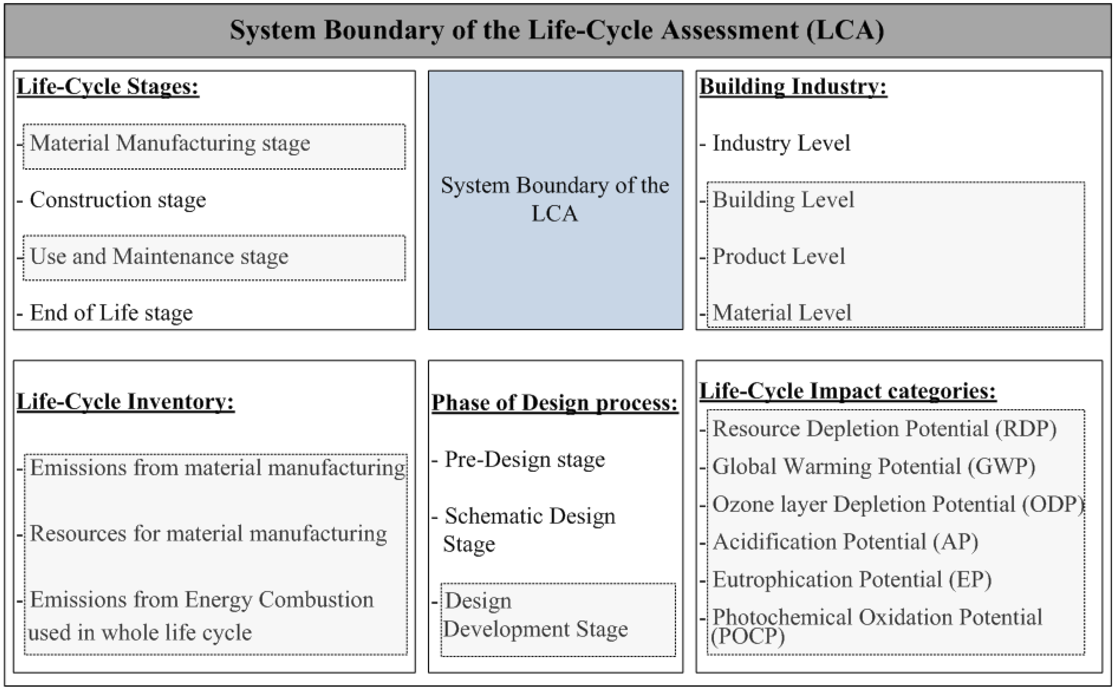
4.1. System Boundary Conditions for Life-Cycle Assessment (LCA) and Life-Cycle Cost (LCC) Analyses

Since the initial investment cost of the GSHP system is quite expensive, the feasibility study needs to be conducted from the life-cycle perspective. Moreover, in recent years, environmental implication has become one of the primary concerns of many governments. Therefore, this study conducted the life-cycle environmental and economic assessment and the following two methods were used: (i) Life-cycle assessment (LCA), a method of calculating the environmental impacts throughout the whole life cycle of a product; (ii) Life-cycle cost (LCC) analysis, a method of calculating the economic value throughout the whole life cycle of a product.

Table 3. Scenarios (length of borehole) of ground heat exchanger (GHE) taking into consideration (entering water temperature) EWT (23 °C) and characteristics of borehole.

Maximum Entering Water Temperature: 23 °C, Minimum Entering Water Temperature: 5 °C
Number of Boreholes: Arrangement (U)	Borehole Spacing	Grout Conductivity (W/mK)	U-Tube Type and Size				U-Tube Type and Size				U-Tube Type and Size
			PN10, DN25				PN10, DN32				PN10, DN40
			Borehole Diameter				Borehole Diameter				Borehole Diameter
			125 mm		150 mm		125 mm		150 mm		125 mm		150 mm
			U-Pipe Spacing				U-Pipe Spacing				U-Pipe Spacing
			3 mm	20 mm	3 mm	20 mm	3 mm	20 mm	3 mm	20 mm	3 mm	20 mm	3 mm	20 mm
22 (EA): 8 × 8	4 m	1 W/mK	249.1	227.3	251.9	232.6	212.1	194.1	215.1	198.7	182.5	168.3	185.2	173.3
		1.4 W/mK	216.7	196.9	217.7	199.7	189.0	174.6	189.8	177.1	166.2	154.2	167.0	156.5
		1.8 W/mK	195.8	181.1	195.8	182.4	174.7	162.1	166.6	163.0	155.8	145.3	155.2	145.9
	5 m	1 W/mK	247.6	225.4	250.5	231.1	210.4	192.5	213.4	197.2	180.3	166.0	183.1	170.8
		1.4 W/mK	214.9	195.2	216.1	198.1	187.3	172.2	188.2	174.8	164.0	152.2	164.8	154.4
		1.8 W/mK	194.4	179.0	194.3	180.2	172.3	159.8	172.0	160.7	153.8	143.6	153.3	144.2
	6 m	1 W/mK	246.6	224.0	249.5	229.9	209.1	191.4	207.8	195.8	179.2	165.1	181.9	169.7
		1.4 W/mK	212.8	194.3	214.7	196.9	186.0	171.1	182.3	173.9	163.0	151.1	163.8	153.4
		1.8 W/mK	193.2	177.9	193.1	179.0	171.5	158.7	166.6	159.6	152.7	142.5	152.2	143.1

Table 3. Scenarios (length of borehole) of ground heat exchanger (GHE) taking into consideration (entering water temperature) EWT (23 °C) and characteristics of borehole.

Maximum Entering Water Temperature: 23 °C, Minimum Entering Water Temperature: 5 °C
Number of Boreholes: Arrangement (U)	Borehole Spacing	Grout Conductivity (W/mK)	U-Tube Type and Size				U-Tube Type and Size				U-Tube Type and Size
			PN10, DN25				PN10, DN32				PN10, DN40
			Borehole Diameter				Borehole Diameter				Borehole Diameter
			125 mm		150 mm		125 mm		150 mm		125 mm		150 mm
			U-Pipe Spacing				U-Pipe Spacing				U-Pipe Spacing
			3 mm	20 mm	3 mm	20 mm	3 mm	20 mm	3 mm	20 mm	3 mm	20 mm	3 mm	20 mm
22 (EA): 8 × 8	4 m	1 W/mK	249.1	227.3	251.9	232.6	212.1	194.1	215.1	198.7	182.5	168.3	185.2	173.3
		1.4 W/mK	216.7	196.9	217.7	199.7	189.0	174.6	189.8	177.1	166.2	154.2	167.0	156.5
		1.8 W/mK	195.8	181.1	195.8	182.4	174.7	162.1	166.6	163.0	155.8	145.3	155.2	145.9
	5 m	1 W/mK	247.6	225.4	250.5	231.1	210.4	192.5	213.4	197.2	180.3	166.0	183.1	170.8
		1.4 W/mK	214.9	195.2	216.1	198.1	187.3	172.2	188.2	174.8	164.0	152.2	164.8	154.4
		1.8 W/mK	194.4	179.0	194.3	180.2	172.3	159.8	172.0	160.7	153.8	143.6	153.3	144.2
	6 m	1 W/mK	246.6	224.0	249.5	229.9	209.1	191.4	207.8	195.8	179.2	165.1	181.9	169.7
		1.4 W/mK	212.8	194.3	214.7	196.9	186.0	171.1	182.3	173.9	163.0	151.1	163.8	153.4
		1.8 W/mK	193.2	177.9	193.1	179.0	171.5	158.7	166.6	159.6	152.7	142.5	152.2	143.1

Table 4. Target scenarios (length of borehole) of GHE considering EWT and characteristics of borehole.

Number of Scenario	Max./Min. Entering Water Temperature	Number of Boreholes: Arrangement (U)	Borehole Spacing	Grout Conductivity (W/mK)	U-Tube Type and Size	Borehole Diameter	U-Pipe Spacing	Borehole Length
Scenario #1	30/5 °C	22 (EA): 8 × 8	6 m	1.8 W/mK	PN10, DN25	150 mm	20 mm	90 m
Scenario #2	27/5 °C							107 m
Scenario #3	25/5 °C							123 m
Scenario #4 (exist GHE)	23/5 °C							143 m
Scenario #5	20/5 °C							195 m

Table 4. Target scenarios (length of borehole) of GHE considering EWT and characteristics of borehole.

Number of Scenario	Max./Min. Entering Water Temperature	Number of Boreholes: Arrangement (U)	Borehole Spacing	Grout Conductivity (W/mK)	U-Tube Type and Size	Borehole Diameter	U-Pipe Spacing	Borehole Length
Scenario #1	30/5 °C	22 (EA): 8 × 8	6 m	1.8 W/mK	PN10, DN25	150 mm	20 mm	90 m
Scenario #2	27/5 °C							107 m
Scenario #3	25/5 °C							123 m
Scenario #4 (exist GHE)	23/5 °C							143 m
Scenario #5	20/5 °C							195 m

4.1.1. Establishment of System Boundary and Assumptions for LCA

To assess the life-cycle environmental effect, the LCA process was conducted by following four steps defined by ISO 14040: (i) Goal and scope definition; (ii) Life-cycle inventory (LCI) analysis; (iii) Life-cycle impact assessment (LCIA); (iv) Results and interpretations [70,71,72]. The system boundary of the LCA showed the depth and breadth as follows (refer to Figure 4): (i) Life-cycle stages (including material manufacturing, use and maintenance stage); (ii) Building industry (including building level, product level, and material level); (iii) Life-cycle inventory (including emissions from material manufacturing, resources use for material manufacturing, and emissions from energy combustion used in whole life cycle); (iv) Phase of design process (including design development stage); (v) Life-cycle impact categories (including RDP, GWP, ODP, AP, EP, and POCP).

Figure 4. System boundary of the LCA.

Figure 4. System boundary of the LCA.

•

Step 1. Goal and scope definition: Based on the information available in whole life cycle, environmental impact generated from the material manufacturing phase and use and maintenance stage are analyzed. The functional unit is defined as “the entire building supplied from design and use and maintenance for a whole service life”.

•

Step 2. LCI analysis: Using the LCI analysis results by life-cycle phase, the environmental-impact substances can be calculated. First, using input-output (I-O) LCA, energy source quantity utilized to produce the material for each life-cycle phase was calculated. Second, employing a process-based LCA, the national LCI database of South Korea established that the environmental-impact substances produced in the material and energy production process can be calculated (refer to Equation (5)) [71,72].

$$E_i={\displaystyle \sum _k(Q{E}_k\times E{P}_{ik}}+Q{E}_k\times E{C}_{ik})$$

(5)

where E_i is the emission of substance (i), QE_k is the quantity of energy source (k), EP_ik is the emission factor of substance (i) emitted in producing one unit of energy source (k), and EC_ik is the emission factor of substance (i) emitted in consuming one unit of energy source (k).

•

Step 3. Life-cycle impact assessment: LCIA converts the environmental-impact substances from the LCI analysis into the environmental impacts. LCIA is made up four categories: (i) Classification; (ii) Characterization; (iii) Normalization; (iv) Weighting [70,71]. In this study, classification and characterization were used to calculate the characterized environmental impact. The process of classification and characterization was calculated by Equation (6) [71,72]. To calculate characterized impacts (CCI_l), the characterization factor (CF_l,i) of each substance is required. Based on the “environmental labeling type III” standard, the characterized environmental impacts on six environmental-impact categories (i.e., RDP, GWP, ODP, AP, EP, and POCP) were presented.

$$CC{I}_l={\displaystyle \sum _i{E}_i\times C{F}_{l,i}}$$

(6)

where CCI_l is the characterized impact of impact category (l), E_i is the emission of substance (i), and CF_l,i is the characterization factor of substance (i) to impact category (l).

•

Step 4. Results and interpretations: Using the estimated environmental impact, environmental and economic values are calculated. Environmental cost signifies the cost generated using end-point LCA methodology [70,73,74]. In this study, the environmental-cost conversion factor proposed in EPS 2000 was used to convert the environmental impact to environmental cost [75] (refer to

Table A5. Environmental cost conversion factor.

Environmental Impact	Environmental Cost Conversion Factor
resource depletion potential (RDP)	2.439 US$/kg-Sb-eq
global warming potential (GWP)	0.167 US$/kg-CO2-eq
ozone layer depletion potential (ODP)	145.172 US$/kg-CFC11-eq
acidification potential (AP)	0.032 US$/kg-SO2-eq
eutrophication potential (EP)	0.029 US$/kg-PO43-eq
photochemical oxidation potential (POCP)	2.675 US$/kg-C2H4-eq

). By analyzing the relative degree of the impact on the global environment of the environmental-impact categories, all the environmental impacts can be converted into environmental cost.

4.1.2. Establishment of System Boundary and Assumptions for LCC

For the calculation of the life-cycle economic value using LCC analysis, the following system boundaries and assumptions were established: (i) analysis approach; (ii) analysis period; (iii) interest rate; and (iv) significant cost of ownership (refer to

Table A6. Boundary conditions of LCC and LCA.

Classification	Detailed Classification	Detailed Description
Analysis Approach		Present Worth Method (NPV40)
Analysis Period		40 years
Realistic Discount Rate	Interest	3.30%
	Electricity	0.66%
	Gas	0.11%
	KCERs	2.66%
Significant Cost of Ownership	Initial construction cost	Initial investment cost
	Operation and maintenance cost	Replacement/repair cost
		Energy consumption cost
	Operation and maintenance benefit	Gas savings, electricity savings
		Benefit from KCERs

) [71].

•

Analysis approach: For the analysis approach, net present value (NPV) was selected for the LCC analysis. NPV is the method used to convert the future value of a design alternative into the present value by considering the discount rate and the time value (refer to Equation (7)). If NPV > 0, the project is deemed feasible; if NPV = 0, the break-even point is deemed to have been reached [76].

$$NPV={\displaystyle \sum _{t=0}^n\frac{BE{S}_t+BE{T}_t}{{\left(1+r\right)}^t}}-{\displaystyle \sum _{t=0}^n\frac{C{I}_t+CR{r}_t+CR{t}_t}{{\left(1+r\right)}^t}}$$

(7)

where NPV is the net present value, BES_t is the benefit from the energy savings in year t, BET_t is the benefit from the emissions trading in year t, CI_t is the cost of the initial investment in year t, CRr_t is the cost of the repair in maintenance phase in year t, CRt_t is the cost of the replacement in maintenance phase in year t, r is the real discount rate, and n is the period of the life-cycle analysis.

•

Analysis period: Generally, the analysis period for the LCC analysis can be established based on the service life of a product, which is based on the building’s structural type [71]. In this study, a 40-year time frame was used for the analysis period of the LCC.

•

Interest rate (refer to Equation (8)): In this study, the real discount rate was calculated using the nominal interest rate and various inflation rates (refer to Table A6) [71]. It can be used for converting various benefits and costs into present values.

$$i=\frac{(1+i_n)}{(1+f)}-1$$

(8)

where i is the real discount rate, i_n is the nominal interest rate, and f is the inflation rate (i.e., electricity price growth rate, gas price growth rate, carbon dioxide emission trading price growth rate).

•

Significant cost of ownership: From the life-cycle perspective, the initial investment cost and the use and maintenance cost need to be considered. The material consumption information was collected from the bill of quantities of the GHE and heat pump. The energy consumption information, on the other hand, was established through energy simulation, which was allocated to the energy cost among the use costs. Meanwhile, the repair rate, repair cycle, and replacement cycle of each material should be considered to calculate the cost in the maintenance phase. In this study, resources such as “Public Procurement Service”, “Ministry of National Defense” and “Implementing Regulations of the Housing Act in Korea (Appendix 5)”, which are provided by respectable institutions, were used [71].

4.2. Optimal GHE in Terms of Environmental and Economic Effects

Among the 540 GHE design alternatives (U arrangement and 22 EA borehole) (refer to Table 3 and Table A1, Table A2, Table A3 and Table A4), the analysis results of five scenarios including existing GHE system are presented as an example (refer to Table 4). As shown in Table 4, the existing GHE (scenario #4) has a maximum EWT of 23 °C and the characteristics of the borehole are 22 EA boreholes, 6 m borehole spacing, 1.8 W/mK grout conductivity and 143 m borehole length. For a direct comparison with the existing GHE (Scenario #4), GHE scenarios were selected on the basis of borehole length according to a change in EWT; furthermore, the characteristics of the borehole except for the length were fixed to analyze the change.

Table 5 shows the results of the design alternative analysis on the GHE in the target facility. The analysis results can be presented in the following three aspects: (i) life-cycle environmental cost; (ii) life-cycle economic cost; and (iii) life-cycle environmental and economic cost. Table A6 shows the boundary conditions of LCC and LCA.

•

First, life-cycle environmental cost: Saving effect of life-cycle environmental cost of Scenario #3 was determined at 2.2% compared with the existing GHE (Scenario #4). Although the initial investment environmental cost is higher than that of the existing GHE, the operation and maintenance environmental cost is lower than that of the existing GHE.

Table 5. Life-cycle environmental and economic cost of scenarios.

Scenario	Classification	Environmental Impact Category						Environmental Cost	Economic Cost	Total Cost
		RDP	GWP	ODP	AP	EP	POCP
		(kg-Sb-eq)	(kg-CO2-eq)	(kg-CFC11-eq)	(kg-SO2-eq)	(kg-PO43-eq)	(kg-C2H4-eq)
Scenario #1	Initial cost	260	151,144	-	804	62	227	23,136	94,638	117,774
	O and M cost	1275	724,427	-	1244	231	2	108,246	104,664	212,909
	Total cost	1535	875,572	-	2047	293	229	131,381	199,302	330,683
Scenario #2	Initial cost	288	168,762	-	898	69	250	25,819	103,296	129,115
	O and M cost	1150	653,432	-	1122	209	2	97,638	96,079	193,716
	Total cost	1437	822,194	-	2020	277	252	123,457	199,375	322,831
Scenario #3	Initial cost	315	186,416	-	993	76	274	28,508	111,969	140,477
	O and M cost	1096	622,723	-	1069	199	2	93,049	92,421	185,469
	Total cost	1411	809,139	-	2062	275	276	121,557	204,390	325,947
Scenario #4	Initial cost	352	210,223	-	1121	85	305	32,133	123,610	155,743
	O and M cost	1085	616,970	-	1059	197	2	92,189	91,824	184,014
	Total cost	1437	827,193	-	2180	282	307	124,322	215,434	339,756
Scenario #5	Initial cost	439	265,811	-	1419	107	379	40,600	150,977	191,578
	O and M cost	966	549,094	-	943	175	2	82,047	83,713	165,760
	Total cost	1405	814,905	-	2362	282	381	122,647	234,690	357,337

Notes: Unit (US$); operation and maintenance phase (O and M); resource depletion potential (RDP); global warming potential (GWP); ozone layer depletion potential (ODP); acidification potential (AP); eutrophication potential (EP); and photochemical oxidation potential (POCP).

Table 5. Life-cycle environmental and economic cost of scenarios.

Scenario	Classification	Environmental Impact Category						Environmental Cost	Economic Cost	Total Cost
		RDP	GWP	ODP	AP	EP	POCP
		(kg-Sb-eq)	(kg-CO2-eq)	(kg-CFC11-eq)	(kg-SO2-eq)	(kg-PO43-eq)	(kg-C2H4-eq)
Scenario #1	Initial cost	260	151,144	-	804	62	227	23,136	94,638	117,774
	O and M cost	1275	724,427	-	1244	231	2	108,246	104,664	212,909
	Total cost	1535	875,572	-	2047	293	229	131,381	199,302	330,683
Scenario #2	Initial cost	288	168,762	-	898	69	250	25,819	103,296	129,115
	O and M cost	1150	653,432	-	1122	209	2	97,638	96,079	193,716
	Total cost	1437	822,194	-	2020	277	252	123,457	199,375	322,831
Scenario #3	Initial cost	315	186,416	-	993	76	274	28,508	111,969	140,477
	O and M cost	1096	622,723	-	1069	199	2	93,049	92,421	185,469
	Total cost	1411	809,139	-	2062	275	276	121,557	204,390	325,947
Scenario #4	Initial cost	352	210,223	-	1121	85	305	32,133	123,610	155,743
	O and M cost	1085	616,970	-	1059	197	2	92,189	91,824	184,014
	Total cost	1437	827,193	-	2180	282	307	124,322	215,434	339,756
Scenario #5	Initial cost	439	265,811	-	1419	107	379	40,600	150,977	191,578
	O and M cost	966	549,094	-	943	175	2	82,047	83,713	165,760
	Total cost	1405	814,905	-	2362	282	381	122,647	234,690	357,337

Notes: Unit (US$); operation and maintenance phase (O and M); resource depletion potential (RDP); global warming potential (GWP); ozone layer depletion potential (ODP); acidification potential (AP); eutrophication potential (EP); and photochemical oxidation potential (POCP).

•

Second, life-cycle economic cost: Saving effect of life-cycle economic cost of Scenario #1 was determined to be 7.5% as compared to the existing GHE (Scenario #4). Although the initial investment cost is higher than that of the existing GHE, the operation and maintenance cost is lower than that of the existing GHE.

•

Third, life-cycle environmental and economic cost: Saving effect of total cost of Scenario #2 was determined to be 5.0% compared with the existing GHE (Scenario #4). Although the initial investment cost is higher than that of the existing GHE, the operation and maintenance cost is lower than that of the existing GHE.

In conclusion, compared to the existing design, the design alternatives of GHE in the target facility were shown to be advantageous in the life-cycle environmental and economic aspects. All of the initial costs tend to decrease when max EWT decreases; however, all of the O and M costs tend to increase when max EWT increases. In other words, as the amount of EWT that enters a heat pump is reduced during the summer, the efficiency of a heat pump becomes higher and borehole length becomes greater.

5. Conclusions

This study aims to assess the environmental and economic effects of the use of GHE for selecting the optimal GHE. This study was undertaken in three steps: (i) establishing the basic information and selecting key factors affecting GHE performances; (ii) making possible alternatives of the GHE installation by considering EWT; and (iii) using life-cycle assessment and life-cycle cost for a comprehensive evaluation of the environmental and economic effects on the GHE.

By conducting a multilateral analysis on the results of the energy simulation, the energy generation effect considering EWT was evaluated by applying the GSHP system. Furthermore, LCA (e.g., RDP, GWP, ODP, AP, EP, and POCP) with the analysis of the LCC was conducted to assess the environmental and economic effects of the implementation of the GSHP system to “Y” university gym facility using NPV methods (refer to Table A6). The analysis results can be summarized as follows:

•

Life-cycle environmental cost: Saving effect of life-cycle environmental cost of Scenario #3 was determined to be 2.2% compared with existing GHE (Scenario #4).

•

Life-cycle economic cost: Saving effect of life-cycle economic cost of Scenario #1 was determined at 7.5% compared with existing GHE (Scenario #4).

•

Life-cycle environmental and economic cost: Saving effect of total cost of scenario #2 was determined at 5.0% compared with existing GHE (Scenario #4).

In conclusion, all of the initial costs tend to decrease when max EWT (for cooling system) decreases; however, all of the O and M costs tend to increase when max EWT increases. In other words, as there is less EWT entering a heat pump during the summer, the efficiency of a GSHP system increases and the borehole lengthens.

The results of this study could benefit potential GSHP system users and give new value in terms of system application in several ways: (i) decide which location is proper for the implementation of the GSHP system considering the characteristics of the regional factor; (ii) maximize the environmental and economic benefit and the efficiency by considering key design factors such as EWT and characteristics of borehole.

Meanwhile, the following research is recommended for future studies: (i) sensitivity analysis of the GSHP system considering the recent trends in the reduction of the initial investment cost and government’s subsidy; (ii) a multi-objective optimization system for the ultimate decision maker to analyze uncountable scenarios in terms of several key factors (EWT and characteristics of borehole).

References

- Korea Energy Management Corporation (KEMCO). 2013 Annual End-Use Energy Statistics. Available online: http://www.kemco.or.kr/ (accessed on 28 June 2015).
- Maria, B. Energy concept design of zero energy buildings. Adv. Mater. Res. 2013, 649, 7–10. [Google Scholar]
- Koo, C.; Hong, T.; Park, H.S.; Yun, G. Framework for the analysis of the potential of the rooftop photovoltaic system to achieve the net-zero energy solar buildings. Prog. Photovolt. Res. Appl. 2014, 22, 462–478. [Google Scholar] [CrossRef]
- Saman, W.Y. Towards zero energy homes down under. Renew. Energy 2013, 49, 211–215. [Google Scholar] [CrossRef]
- Li, D.H.; Yang, L.; Lam, J.C. Zero energy buildings and sustainable development implications—A review. Energy 2013, 54, 1–10. [Google Scholar] [CrossRef]
- Hong, T.; Koo, C.; Kwak, T. Framework for the implementation of a new renewable energy system in an educational facility. Appl. Energy 2013, 103, 539–551. [Google Scholar] [CrossRef]
- Hong, T.; Koo, C.; Kwak, T.; Park, H.S. An economic and environmental assessment for selecting the optimal new renewable energy system for educational facility. Renew. Sustain. Energy. Rev. 2014, 29, 286–300. [Google Scholar] [CrossRef]
- Hong, T.; Koo, C.; Park, J.; Park, H.S. A GIS (geographic information system)-based optimization model for estimating the electricity generation of the rooftop PV (photovoltaic) system. Energy 2014, 65, 190–199. [Google Scholar] [CrossRef]
- Hearps, P.; McConnell, D. Renewable Energy Technology Cost Review; Melbourne Energy Institute: Carlton, Victoria, Australia, 2011. [Google Scholar]
- International Energy Agency. Medium-Term Renewable Energy Market Report 2012; OECD Publishing: Paris, France, 2012. [Google Scholar]
- Renewables 2012: Global Status Report; Renewable Energy Policy Network for the 21st Century: Paris, France, 2012.
- World Energy Outlook 2012; International Energy Agency: Paris, France, 2012.
- World Energy Outlook 2013; International Energy Agency: Paris, France, 2013.
- World Energy Outlook 2014; International Energy Agency: Paris, France, 2014.
- Hwang, Y.; Lee, J.K.; Jeong, Y.M.; Koo, K.M.; Lee, D.H.; Kim, I.K.; Kim, S.H. Cooling performance of a vertical ground-coupled heat pump system installed in a school building. Renew. Energy 2009, 34, 578–582. [Google Scholar] [CrossRef]
- Gao, Q.; Li, M.; Yu, M.; Spitler, J.D.; Yan, Y.Y. Review of development from GSHP to UTES in China and other countries. Renew. Sustain. Energy Rev. 2009, 13, 1383–1394. [Google Scholar] [CrossRef]
- Dalla Rosa, A.; Christensen, J.E. Low-energy district heating in energy-efficient building areas. Energy 2011, 36, 6890–6899. [Google Scholar] [CrossRef]
- Aikins, K.A.; Choi, J.M. Current status of the performance of GSHP (ground source heat pump) units in the Republic of Korea. Energy 2012, 47, 77–82. [Google Scholar] [CrossRef]
- Kharseh, M.; Nordell, B. Sustainable heating and cooling systems for agriculture. Int. J. Energy Res. 2011, 35, 415–422. [Google Scholar] [CrossRef]
- Li, S.F.; Shang, Y.; Chen, D. The numerical study on the environmentally sustainable system-ground-source heat pump system. Adv. Mater. Res. 2011, 320, 530–535. [Google Scholar] [CrossRef]
- Hepbasli, A. A key review on exergetic analysis and assessment of renewable energy resources for a sustainable future. Renew. Sustain. Energy Rev. 2008, 12, 593–661. [Google Scholar] [CrossRef]
- Hyysalo, S.; Juntunen, J.K.; Freeman, S. User innovation in sustainable home energy technologies. Energy Policy 2013, 55, 490–500. [Google Scholar] [CrossRef]
- Kaygusuz, K.; Kaygusuz, A. Geothermal energy in Turkey: The sustainable future. Renew. Sustain. Energy Rev. 2004, 8, 545–563. [Google Scholar] [CrossRef]
- Healy, P.F.; Ugursal, V.I. Performance and economic feasibility of ground source heat pumps in cold climate. Int. J. Energy Res. 1997, 21, 857–870. [Google Scholar] [CrossRef]
- Omer, A.M. Clean energies for sustainable development for built environment. J. Civ. Eng. Constr. Technol. 2012, 3, 1–16. [Google Scholar] [CrossRef]
- Ozudogru, T.Y.; Ghasemi-Fare, O.; Olgun, C.G.; Basu, P. Numerical modeling of vertical geothermal heat exchangers using finite difference and finite element techniques. Geotech. Geol. Eng. 2015, 33, 291–306. [Google Scholar] [CrossRef]
- Guo, Y.; Zhang, G.; Zhou, J.; Wu, J.; Shen, W. A techno-economic comparison of a direct expansion ground-source and a secondary loop ground-coupled heat pump system for cooling in a residential building. Appl. Therm. Eng. 2012, 35, 29–39. [Google Scholar] [CrossRef]
- Sanner, B.; Karytsas, C.; Mendrinos, D.; Rybach, L. Current status of ground source heat pumps and underground thermal energy storage in Europe. Geothermics 2003, 32, 579–588. [Google Scholar] [CrossRef]
- Ozgener, O.; Hepbasli, A. Modeling and performance evaluation of ground source (geothermal) heat pump systems. Energy Build. 2007, 39, 66–75. [Google Scholar] [CrossRef]
- Hepbasli, A. Exergetic modeling and assessment of solar assisted domestic hot water tank integrated ground-source heat pump systems for residences. Energy Build. 2007, 39, 1211–1217. [Google Scholar] [CrossRef]
- Badescu, V. Economic aspects of using ground thermal energy for passive house heating. Renew. Energy 2007, 32, 895–903. [Google Scholar] [CrossRef]
- Bichiou, Y.; Krarti, M. Optimization of envelope and HVAC systems selection for residential buildings. Energy Build. 2011, 43, 3373–3382. [Google Scholar] [CrossRef]
- Ghasemi-Fare, O.; Basu, P. A practical heat transfer model for geothermal piles. Energy Build. 2013, 66, 470–479. [Google Scholar] [CrossRef]
- Dieckmann, J. Heat pumps for cold climates. ASHRAE J. 2009, 51, 69–72. [Google Scholar]
- Ni, L.; Song, W.; Zeng, F.; Yao, Y. Energy Saving and Economic Analyses of Design Heating Load Ratio of Ground Source Heat Pump with Gas Boiler as Auxiliary Heat Source. In Proceedings of the International Conference on Electric Technology and Civil Engineering, Jiujiang, China, 22–24 April 2011.
- Genchi, Y.; Kikegawa, Y.; Inaba, A. CO2 payback-time assessment of a regional-scale heating and cooling system using a ground source heat-pump in a high energy-consumption area in Tokyo. Appl. Energy 2002, 71, 147–160. [Google Scholar] [CrossRef]
- Blum, P.; Campillo, G.; Münch, W.; Kölbel, T. CO2 savings of ground source heat pump systems—A regional analysis. Renew. Energy 2010, 35, 122–127. [Google Scholar] [CrossRef]
- Saner, D.; Juraske, R.; Kübert, M.; Blum, P.; Hellweg, S.; Bayer, P. Is it only CO2 that matters? A life cycle perspective on shallow geothermal systems. Renew. Sustain. Energy Rev. 2010, 14, 1798–1813. [Google Scholar] [CrossRef]
- Dong, H.; Geng, Y.; Xi, F.; Fujita, T. Carbon footprint evaluation at industrial park level: A hybrid life cycle assessment approach. Energy Policy 2013, 57, 298–307. [Google Scholar] [CrossRef]
- Hamada, Y.; Nakamura, M.; Ochifuji, K.; Nagano, K.; Yokoyama, S. Field performance of a Japanese low energy home relying on renewable energy. Energy Build. 2001, 33, 805–814. [Google Scholar] [CrossRef]
- Greening, B.; Azapagic, A. Domestic heat pumps: Life cycle environmental impacts and potential implications for the UK. Energy 2012, 39, 205–217. [Google Scholar] [CrossRef]
- Katsura, T.; Nagano, K.; Takeda, S. Method of calculation of the ground temperature for multiple ground heat exchangers. Appl. Therm. Eng. 2008, 28, 1995–2004. [Google Scholar] [CrossRef]
- Troldborg, M.; Heslop, S.; Hough, R.L. Assessing the sustainability of renewable energy technologies using multi-criteria analysis: Suitability of approach for national-scale assessments and associated uncertainties. Renew. Sustain. Energy Rev. 2014, 39, 1173–1184. [Google Scholar] [CrossRef]
- Geng, Y.; Sarkis, J.; Wang, X.; Zhao, H.; Zhong, Y. Regional application of ground source heat pump in China: A case of Shenyang. Renew. Sustain. Energy Rev. 2013, 18, 95–102. [Google Scholar] [CrossRef]
- Zhu, Y.; Tao, Y.; Rayegan, R. A comparison of deterministic and probabilistic life cycle cost analyses of ground source heat pump (GSHP) applications in hot and humid climate. Energy Build. 2012, 55, 312–321. [Google Scholar] [CrossRef]
- Sekine, K.; Ooka, R.; Yokoi, M.; Shiba, Y.; Hwang, S. Development of a ground-source heat pump system with ground heat exchanger utilizing the cast-in-place concrete pile foundations of buildings. ASHRAE Trans. 2007, 113, 1–9. [Google Scholar]
- Nagano, K.; Katsura, T.; Takeda, S. Development of a design and performance prediction tool for the ground source heat pump system. Appl. Therm. Eng. 2006, 26, 1578–1592. [Google Scholar] [CrossRef]
- Hamdy, M.; Hasan, A.; Siren, K. A multi-stage optimization method for cost-optimal and nearly-zero-energy building solutions in line with the EPBD-recast 2010. Energy Build. 2013, 56, 189–203. [Google Scholar] [CrossRef]
- Self, S.J.; Reddy, B.V.; Rosen, M.A. Geothermal heat pump systems: Status review and comparison with other heating options. Appl. Energy 2013, 101, 341–348. [Google Scholar] [CrossRef]
- Gao, J.; Zhang, X.; Liu, J.; Li, K.S.; Yang, J. Thermal performance and ground temperature of vertical pile-foundation heat exchangers: A case study. Appl. Therm. Eng. 2008, 28, 2295–2304. [Google Scholar] [CrossRef]
- Hepbasli, A.; Akdemir, O.; Hancioglu, E. Experimental study of a closed loop vertical ground source heat pump system. Energy Convers. Manag. 2003, 44, 527–548. [Google Scholar] [CrossRef]
- Zhang, Q.; Murphy, W.E. Measurement of thermal conductivity for three borehole fill materials used for GSHP. ASHRAE Trans. 2000, 106, 434. [Google Scholar]
- Kharseh, M.; Altorkmany, L.; Nordell, B. Global warming’s impact on the performance of GSHP. Renew. Energy 2011, 36, 1485–1491. [Google Scholar] [CrossRef]
- Lamarche, L.; Kajl, S.; Beauchamp, B. A review of methods to evaluate borehole thermal resistances in geothermal heat-pump systems. Geothermics 2010, 39, 187–200. [Google Scholar] [CrossRef]
- Butler, D.K.; Curro, J.R., Jr. Crosshole seismic testing—Procedures and pitfalls. Geophysics 1981, 46, 23–29. [Google Scholar] [CrossRef]
- Fan, R.; Gao, Y.; Hua, L.; Deng, X.; Shi, J. Thermal performance and operation strategy optimization for a practical hybrid ground-source heat-pump system. Energy Build. 2014, 78, 238–247. [Google Scholar] [CrossRef]
- Zeng, H.; Diao, N.; Fang, Z. Efficiency of vertical geothermal heat exchangers in the ground source heat pump system. J. Therm. Sci. 2003, 12, 77–81. [Google Scholar] [CrossRef]
- Liu, X.L.; Wang, D.L.; Fan, Z.H. Modeling on heat transfer of a vertical bore in geothermal heat exchangers. Build. Energy Environ. 2001, 2, 1–3. [Google Scholar]
- Beier, R.A.; Smith, M.D.; Spitler, J.D. Reference data sets for vertical borehole ground heat exchanger models and thermal response test analysis. Geothermics 2011, 40, 79–85. [Google Scholar] [CrossRef]
- Inalli, M.; Esen, H. Experimental thermal performance evaluation of a horizontal ground-source heat pump system. Appl. Therm. Eng. 2004, 24, 2219–2232. [Google Scholar] [CrossRef]
- Khan, M.A.; Wang, J.X. Development of a graph method for preliminary design of borehole ground-coupled heat exchanger in North Louisiana. Energy Build. 2015, 92, 389–397. [Google Scholar] [CrossRef]
- Jeon, J.; Lee, S.; Hong, D.; Kim, Y. Performance evaluation and modeling of a hybrid cooling system combining a screw water chiller with a ground source heat pump in a building. Energy 2010, 35, 2006–2012. [Google Scholar] [CrossRef]
- Madani, H.; Claesson, J. Retrofitting a variable capacity heat pump to a ventilation heat recovery system: Modeling and performance analysis. In Proceedings of the International Conference on Applied Energy, Singapore, 21–23 April 2010; pp. 649–658.
- Hepbasli, A.; Akdemir, O. Energy and exergy analysis of a ground source (geothermal) heat pump system. Energy Convers. Manag. 2004, 45, 737–753. [Google Scholar] [CrossRef]
- Sivasakthivel, T.; Murugesan, K.; Sahoo, P.K. Potential reduction in CO2 emission and saving in electricity by ground source heat pump system for space heating applications-a study on northern part of India. Procedia Eng. 2012, 38, 970–979. [Google Scholar] [CrossRef]
- Yavuzturk, C.; Spitler, J.D. A short time step response factor model for vertical ground loop heat exchangers. ASHARE Trans. 1999, 105, 475–485. [Google Scholar]
- Yavuzturk, C. Modeling of Vertical Ground Loop Heat Exchangers for Ground Source Heat Pump Systems. Ph.D. Thesis, Oklahoma State University, Stillwater, OK, USA, December 1999. [Google Scholar]
- Spitler, J.D. GLHEPRO—A Design Tool for Commercial Building Ground Loop Heat Exchangers. In Proceedings of the Fourth International Heat Pumps in Cold Climates Conference, Quebec, QC, Canada, 17–18 August 2000.
- Crawley, D.B.; Lawrie, L.K.; Pedersen, C.O.; Liesen, R.J.; Fisher, D.E.; Strand, R.K.; Taylor, R.D.; Winkelmann, F.C.; Buhl, W.F.; Huang, Y.J.; et al. EnergyPlus: A New Generation Building Energy Simulation Program. In Proceedings of the Renewable and Advanced Energy Systems for the 21st Century, Maui, HI, USA, 11–15 April 1999.
- The American Institute of Architects (AIA). A Guide to Life Cycle Assessment of Buildings; AIA: New York, NY, USA, 2010. [Google Scholar]
- Kim, C.J.; Kim, J.; Hong, T.; Koo, C.; Jeong, K.; Park, H.S. A program-level management system for the life cycle environmental and economic assessment of complex building projects. Environ. Impact Assess. 2015, 54, 9–21. [Google Scholar] [CrossRef]
- Jeong, K.; Ji, C.; Koo, C.; Hong, T.; Park, H.S. A model for predicting the environmental impacts of educational facilities in the project planning phase. J. Clean. Prod. 2014. [Google Scholar] [CrossRef]
- Kosareo, L.; Ries, R. Comparative environmental life cycle assessment of green roofs. Build. Environ. 2007, 42, 2606–2613. [Google Scholar] [CrossRef]
- Kumaran, D.S.; Ong, S.K.; Tan, R.B.; Nee, A.Y.C. Environmental life cycle cost analysis of products. Environ. Manag. Health 2001, 12, 260–276. [Google Scholar] [CrossRef]
- Steen, B. A Systematic Approach to Environmental Priority Strategies in Product Development (EPS): Version 2000-General System Characteristics; Chalmers University of Technology: Göteborg, Sweden, 1999. [Google Scholar]
- Koo, C.; Park, S.; Hong, T.; Park, H.S. An estimation model for the heating and cooling demand of a residential building with a different envelope design using the finite element method. Appl. Energy 2014, 115, 205–215. [Google Scholar] [CrossRef]
© 2015 by the authors; licensee MDPI, Basel, Switzerland. This article is an open access article distributed under the terms and conditions of the Creative Commons Attribution license (http://creativecommons.org/licenses/by/4.0/).
Share and Cite
Kim, J.; Hong, T.; Chae, M.; Koo, C.; Jeong, J. An Environmental and Economic Assessment for Selecting the Optimal Ground Heat Exchanger by Considering the Entering Water Temperature. Energies 2015, 8, 7752-7776. https://doi.org/10.3390/en8087752
Kim J, Hong T, Chae M, Koo C, Jeong J. An Environmental and Economic Assessment for Selecting the Optimal Ground Heat Exchanger by Considering the Entering Water Temperature. Energies. 2015; 8(8):7752-7776. https://doi.org/10.3390/en8087752
Chicago/Turabian StyleKim, Jimin, Taehoon Hong, Myeongsoo Chae, Choongwan Koo, and Jaemin Jeong. 2015. "An Environmental and Economic Assessment for Selecting the Optimal Ground Heat Exchanger by Considering the Entering Water Temperature" Energies 8, no. 8: 7752-7776. https://doi.org/10.3390/en8087752
APA StyleKim, J., Hong, T., Chae, M., Koo, C., & Jeong, J. (2015). An Environmental and Economic Assessment for Selecting the Optimal Ground Heat Exchanger by Considering the Entering Water Temperature. Energies, 8(8), 7752-7776. https://doi.org/10.3390/en8087752