Short-Run and Long-Run Elasticities of Diesel Demand in Korea


Abstract
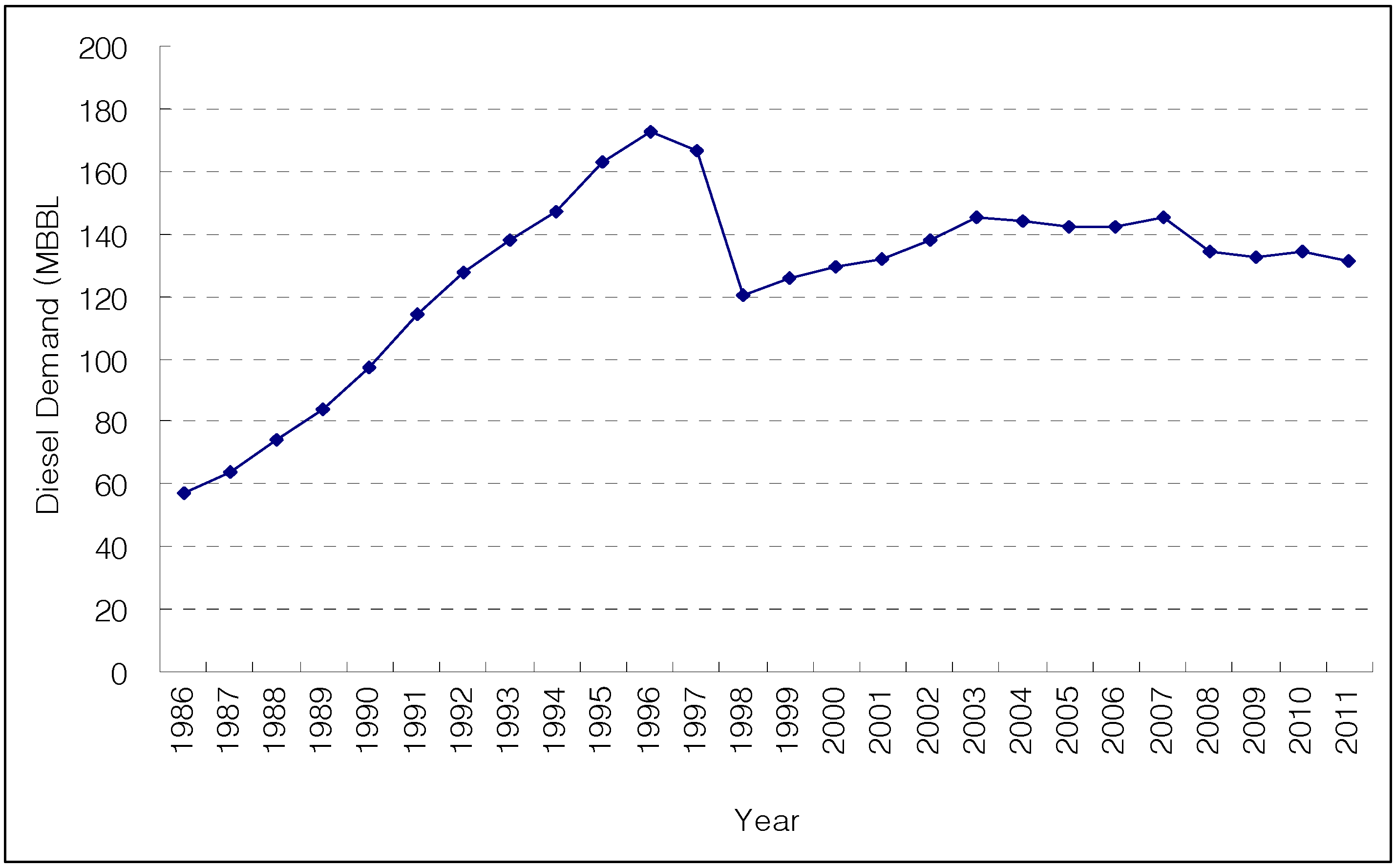
:1. Introduction

| Fuels (Vehicle model) | Engine displacement | Polluting gas emission (g/km) | Official fuel efficiency (km/L) | ||||
|---|---|---|---|---|---|---|---|
| CO | HC | NOX | PM | CO2 | |||
| Diesel (i40 1.7) | 1,685 cc | 0.136 | 0.023 | 0.142 | 0.0001 | 149 | 18.0 |
| Gasoline (sonata 2.0) | 1,999 cc | 0.111 | 0.014 | 0.014 | - | 159 | 14.7 |
| LPG (sonata 2.0) | 1,999 cc | 0.340 | 0.007 | 0.011 | - | 169 | 10.5 |
| Country | Transportation fuel | Period | Long-run elasticity | Short-run elasticity | Sources | ||
|---|---|---|---|---|---|---|---|
| Income | Price | Income | Price | ||||
| Kuwait | Gasoline | 1970–1989 | 0.92 | −0.46 | 0.47 | −0.37 | Eltony [4] |
| GCC | Gasoline | 1975–1993 | 0.48 | −0.17 | 0.31 | −0.11 | Eltony [5] |
| OECD | Gasoline | 1978–2005 | 0.20 | −0.19 | 0.28 | −0.16 | Liddle [7] |
| 0.34 | −0.43 | ||||||
| India | Gasoline | 1972–1994 | 2.68 | −0.32 | 1.18 | −0.21 | Ramanathan [8] |
| OECD | Gasoline | 1960–1985 | 1.17 | −0.79 | 0.41 | −0.24 | Graham et al. [9] |
| Brazil | Gasoline | 1974–1994 | 0.12 | −0.46 | 0.12 | −0.09 | Alves and Bueno [10] |
| Namibia | Diesel | 1980–2002 | 2.08 | −0.11 | - | - | de Vita et al. [11] |
| Greece | Gasoline | 1978–2003 | 0.79 | −0.38 | 0.36 | −0.10 | Polemis [12] |
| Diesel | 1978–2003 | 1.18 | −0.71 | 0.42 | −0.07 | ||
| South Africa | Gasoline | 1978–2005 | 0.36 | −0.47 | - | - | Akinboade et al. [13] |
| Fiji | Gasoline | 1978–2005 | 0.43 | −0.24 | 2.56 | −0.36 | Rao and Rao [14] |
| US | Gasoline | 1976–2008 | 0.07 | −0.25 | - | - | Park et al [15] |
| Senegal | Gasoline | 1970–2008 | 1.14 | −3.01 | 0.46 | −0.12 | Sene [16] |
| Korea | Gasoline | 1996–2010 | 1.40 | −7.40 | 1.26 | −3.81 | Lim and Yoo [17] |
2. Methodology and Data
3. Results and Discussion
3.1. Results of Unit Roots and Co-Integration Tests
| Levels | First-differences | |
|---|---|---|
| D | −20.954 [6] (0.058) | −108.355 [5] * (0.000) |
| Y | −10.658 [4] (0.393) | −80.052 [3] * (0.000) |
| P | −7.814 [3] (0.599) | −84.742 [2] * (0.000) |
| Null hypotheses | Likelihood ratio test statistic | p-values |
|---|---|---|
| H0 (R = 0) | 35.372 * | 0.039 |
| H0 (R ≤ 1) | 17.609 | 0.060 |
| H0 (R ≤ 2) | 2.816 | 0.086 |
3.2. Results of Error-Correction Model
| CUSUM test | CUSUMSQ test | |||
|---|---|---|---|---|
| Test statistic | p-values | Test statistic | p-values | |
| Equation (2) | 0.796 | 0.142 | 0.117 | 0.451 |
| Short-run | Long-run | |
|---|---|---|
| Income elasticity | 1.589 ** (5.12) | 1.478 ** (17.39) |
| Price elasticity | −0.357 ** (−5.49) | −0.547 ** (−13.99) |
4. Conclusion
References
- Jeong, D.S. Report on the clean diesel taxi; Korea Institute of Machinery & Materials: Daejeon, Korea, 2012. [Google Scholar]
- Korean Energy Economics Institute. Yearbook of Energy Statistics; Uiwang-si, Korea, 2012. [Google Scholar]
- Sterner, T. International Energy Economics; Chapman and Hall: London, UK, 1992; pp. 65–79. [Google Scholar]
- Eltony, M.N. Demand for gasoline in Kuwait: An empirical analysis using cointegration techniques. Energy Econ. 1995, 17, 249–253. [Google Scholar] [CrossRef]
- Eltony, M.N. Demand for gasoline in the GCC: An application of pooling and testing procedures. Energy Econ. 1996, 18, 203–209. [Google Scholar] [CrossRef]
- Liddle, B. Long-run relation among transport demand, income, and gasoline price for the US. Transp. Res. D: Transp. Environ. 2009, 14, 73–82. [Google Scholar] [CrossRef]
- Liddle, B. The systemic, long-run relation among gasoline demand, gasoline price, income, and vehicle ownership in OECD countries: Evidence from panel cointegration and causality modeling. Transp. Res. D: Transp. Environ. 2012, 17, 327–331. [Google Scholar] [CrossRef]
- Ramanathan, R. Short-run and long-run elasticities of gasoline demand in India: An empirical analysis using cointegration techniques. Energy Econ. 1999, 21, 321–330. [Google Scholar] [CrossRef]
- Graham, D.J.; Glaister, S. The demand for automobile fuel: a survey of elasticities. J. Transp. Econ. Policy 2002, 36, 1–26. [Google Scholar]
- Alves, D.C.O.; Bueno, R.D.L.S. Short-run, long-run and cross elasticities of gasoline demand in Brazil. Energy Econ. 2003, 25, 191–199. [Google Scholar] [CrossRef]
- de Vita, G.; Endresen, K.; Hunt, L.C. An empirical analysis of energy demand in Namibia. Energy Policy 2006, 34, 3447–3463. [Google Scholar] [CrossRef]
- Polemis, M.L. Empirical assessment of the determinants of road energy demand in Greece. Energy Econ. 2006, 28, 385–403. [Google Scholar] [CrossRef]
- Akinboade, O.A.; Ziramba, E.; Kumo, W.L. The demand for gasoline in South Africa: An empirical analysis using co-integration techniques. Energy Econ. 2008, 30, 3222–3229. [Google Scholar] [CrossRef]
- Rao, B.B.; Rao, G. Cointegration and the demand for gasoline. Energy Policy 2009, 37, 3978–3983. [Google Scholar] [CrossRef]
- Park, S.Y.; Zhao, G. An estimation of U.S. gasoline demand: A smooth time-varying cointegration approach. Energy Econ. 2010, 32, 110–120. [Google Scholar] [CrossRef]
- Sene, S.O. Estimating the demand for gasoline in developing countries: Senegal. Energy Econ. 2012, 34, 189–194. [Google Scholar] [CrossRef]
- Lim, K.M.; Yoo, S.H. Short-run and long-run elasticities of gasoline demand: The case of Korea. Energy Source B Econ. Plan. Policy. in press.
- Dahl, C.A.; Sterner, T. The pricing of and the demand for gasoline: A survey of models. Goteberg University: Memorandum, Sweden, 1990; Volume 132, pp. 1–180. [Google Scholar]
- Granger, C.W.J.; Newbold, P. Spurious regressions in econometrics. J. Econom. 1974, 2, 111–120. [Google Scholar] [CrossRef]
- Stock, J.H.; Watson, M.W. Interpreting the evidence in money-income causality. J. Econom. 1989, 40, 161–182. [Google Scholar] [CrossRef]
- Engle, R.F.; Granger, C.W.J. Cointegration and error correction: representation, estimation and testing. Econometrica 1987, 55, 251–276. [Google Scholar] [CrossRef]
- Dickey, D.A.; Fuller, W.A. Distribution of the estimators for autoregressive time series with a unit root. J. Am. Stat. Assoc. 1979, 74, 427–431. [Google Scholar]
- Said, S.; Dickey, D.A. Testing for unit roots in autoregressive-moving average models of unknown order. Biometrika 1984, 71, 599–607. [Google Scholar] [CrossRef]
- Phillips, P.C.B.; Perron, P. Testing for a unit root in time series regression. Biometrika 1988, 75, 335–346. [Google Scholar] [CrossRef]
- Pantula, S.G.; Gonzalez-Farias, G.; Fuller, W.A. A comparison of unit-root test criteria. J. Bus. Econ. Stat. 1994, 12, 449–459. [Google Scholar] [Green Version]
- Johansen, S.; Juselius, K. Maximum likelihood estimation and inference on cointegration with applications to the demand for money. Oxford Bull. Econ. Stat. 1990, 52, 169–210. [Google Scholar] [CrossRef]
- Park, J.Y. Canoical cointegration regressions. Econometrica 1992, 60, 119–143. [Google Scholar] [CrossRef]
- Brown, R.; Durbin, J.; Evans, J. Techniques for testing the constancy of regression relationships over time. J. R. Stat. Soc. Ser. B 1975, 37, 149–172. [Google Scholar]
- Greene, W.H. Econometric Analysis, 3rd ed.; Prentice-Hall: Saddle River, NJ, USA, 1997. [Google Scholar]
- Ramsey, J.B. Tests for Specification Errors in Classical Linear Least Squares Regression Analysis. J. R. Stat. Soc. Ser. B 1969, 31, 350–371. [Google Scholar]
© 2012 by the authors; licensee MDPI, Basel, Switzerland. This article is an open access article distributed under the terms and conditions of the Creative Commons Attribution license (http://creativecommons.org/licenses/by/3.0/).
Share and Cite
Lim, K.-M.; Kim, M.; Kim, C.S.; Yoo, S.-H. Short-Run and Long-Run Elasticities of Diesel Demand in Korea. Energies 2012, 5, 5055-5064. https://doi.org/10.3390/en5125055
Lim K-M, Kim M, Kim CS, Yoo S-H. Short-Run and Long-Run Elasticities of Diesel Demand in Korea. Energies. 2012; 5(12):5055-5064. https://doi.org/10.3390/en5125055
Chicago/Turabian StyleLim, Kyoung-Min, Myunghwan Kim, Chang Seob Kim, and Seung-Hoon Yoo. 2012. "Short-Run and Long-Run Elasticities of Diesel Demand in Korea" Energies 5, no. 12: 5055-5064. https://doi.org/10.3390/en5125055
APA StyleLim, K.-M., Kim, M., Kim, C. S., & Yoo, S.-H. (2012). Short-Run and Long-Run Elasticities of Diesel Demand in Korea. Energies, 5(12), 5055-5064. https://doi.org/10.3390/en5125055