Study on MPC Regulation Control Strategy Based on Dynamic Characteristics of Heating Systems

Abstract

Driven by the growing energy demand and severe challenges posed by climate change, reducing the high energy consumption of district heating systems while enhancing their flexibility and operational reliability has become an urgent priority. This study focuses on the heating system of a residential community in Zhengzhou, China, by developing a joint source-network-load simulation model and proposing a model predictive control (MPC) strategy tailored to the dynamic characteristics of the system. A white-box model of the building complex and heating system was established by coupling EnergyPlus and Modelica. Subsequently, the model was automatically calibrated using actual operational data and the GenOpt optimization tool, which further improved the simulation accuracy and optimal control performance of the model. The results show that the root mean square errors (RMSEs) of the calibrated secondary network supply water temperature, return water temperature, and indoor temperature decreased by 34.6% and 15.7%, respectively, verifying the effectiveness of the proposed calibration method. Furthermore, the proposed MPC strategy demonstrates significant advantages over conventional control baselines, greatly improving the temperature regulation accuracy and system stability. Compared to the baseline operation without MPC, the proposed strategy increases the user-side thermal comfort index from 56% to 100%, thereby significantly enhancing overall heating quality.

1. Introduction

Amidst rapid technological advancement, global energy demand continues to grow. However, in pursuit of sustainable development, nations worldwide are striving to reduce energy consumption and carbon emissions [1,2]. Controlling energy consumption within the building sector remains a significant challenge, with space heating constituting the primary energy end-use and accounting for approximately 40% of total building energy consumption [3,4]. In recent years, driven by global climate change, extreme temperature events have become increasingly frequent and severe, significantly impacting the built environment and subsequently altering the operational dynamics of heating systems [5,6,7]. To enhance the stability and reliability of heating systems while achieving sustainable, low-carbon operations, a comprehensive understanding of the energy consumption characteristics and dynamic interactions among various components within the heating network is essential.

Numerous studies have developed source-network-load mixed-integer linear programming (MILP) models for district heating and other energy systems [8,9,10]. This modeling approach facilitates the optimization of equipment selection and capacity sizing while incorporating factors such as heating network hydraulic regulation, water pump energy consumption, and building heat load, thereby optimizing overall system performance.

Among these components, the heating system plays a pivotal role in optimizing energy utilization efficiency. Several studies [11,12,13] have investigated the optimization of renewable-based heat source systems and proposed hybrid models, thereby enhancing system flexibility and sustainability. Existing research demonstrates that effective heat source modeling must account for not only individual energy source optimization but also the complementary characteristics of multiple energy sources to achieve superior energy efficiency.

Operational monitoring and the regulation of heating networks often rely on design parameters; however, models based solely on design conditions fail to accurately reflect actual operating conditions. Consequently, extensive research has been conducted on the simulation and modeling of these networks. Software tools such as MATLAB R2025a [14,15], CFD [16,17] and Dymola [18] are commonly utilized for network modeling to analyze fluid dynamics and energy efficiency. To better capture actual network operations, researchers have proposed various advanced modeling approaches. For instance, Li et al. [19] proposed a quasi-dynamic model to estimate the hydraulic and thermal behavior of district heating networks, demonstrating improved accuracy and reduced computational time. Calixto et al. [20] utilized pre-design support tools from the Flexynets project for the preliminary modeling and data analysis of an existing neutral-temperature district heating network, achieving an overall deviation of 15% for key performance indicators. Xu et al. [21] introduced a novel TOTS layout method for district heating systems and established a corresponding three-dimensional numerical simulation model, which exhibited high accuracy with a deviation of less than 2%. Vieth et al. [22] developed a specialized algorithm that generates optimal network topologies based on real geo-referenced data and automatically constructs simulation models to determine the ideal network configuration. Furthermore, Meibodi et al. [23] formulated a model to rapidly and accurately simulate the dynamic thermal behavior of buried pipelines, featuring both high accuracy and computational efficiency. Collectively, these advanced methodologies significantly enhance the practicality and reliability of heating network modeling.

Load-side modeling is critical for enabling demand response and achieving energy savings in heating systems. Yang et al. [24] extensively investigated load model development and proposed various methodologies, including load forecasting and energy consumption indices. By incorporating user comfort preferences, Moradzadeh et al. [25] established a behavior-based load model that more accurately predicts energy consumption patterns, thereby providing a robust foundation for demand response and load management. Yan et al. [26] proposed a multi-objective, two-stage adaptive robust programming method to address load uncertainty in integrated energy systems. Their findings demonstrate that precise load-side modeling facilitates better prediction of and response to user demand, thereby achieving optimal scheduling and energy savings. Furthermore, by introducing machine learning techniques, Potočni et al. [27] significantly improved the accuracy and reliability of load forecasting. Collectively, these studies indicate that effective load-side modeling must incorporate not only basic energy requirements but also user behavior and comfort preferences to achieve precise demand response and energy management.

As heating systems grow increasingly complex, numerous scholars [27,28,29,30,31] have focused on dynamic modeling and optimization methods, achieving more efficient resource allocation and energy consumption management by simulating system dynamics. These studies demonstrate that dynamic modeling and optimization techniques offer significant advantages in managing the inherent complexity and uncertainty of heating systems, providing a more accurate representation of network operating states.

In recent years, model predictive control (MPC) has garnered increasing attention and application in heating systems as an advanced control strategy. It is primarily employed for algorithm optimization and robustness analysis. Facilities characterized by significant thermal inertia and load fluctuations, such as large office buildings and hospitals, have emerged as primary application scenarios for MPC [32]. Within this domain, researchers have proposed various models and algorithms to enhance the efficiency and stability of heating systems. For example, improved particle swarm optimization (PSO) algorithms have been utilized to optimize scheduling strategies, iteratively adjusting the operating parameters of energy supply systems based on load forecasting results to achieve energy-saving operations [33,34]. Additionally, novel optimization algorithms such as the longhorn beetle swarm search algorithm have been introduced for building thermal load forecasting. Compared to traditional genetic algorithms and standard PSO, these novel approaches offer distinct advantages in forecasting accuracy and computational efficiency [35,36,37]. Furthermore, advanced deep learning and reinforcement learning algorithms have recently been applied to the operation of smart heating systems. For instance, CNN-based models can achieve precise thermal load forecasting for building complexes, providing robust technical support for the optimal control of district heating networks [38,39,40]. Moreover, distributed optimization algorithms improve overall heating network performance by implementing local optimization at individual nodes or subsystems. Studies [41,42,43] have demonstrated that these distributed approaches possess significant advantages in managing the complexity and dynamic variations inherent in heating systems.

In summary, existing research has achieved notable progress in specific domains, including outdoor pipe network hydraulic modeling, building model predictive control, and local adjustment strategies. Nevertheless, there remains a critical lack of systematic research concerning the comprehensive modeling, dynamic simulation, and holistic optimal control of the entire source-network-load chain, particularly under conditions of flexible load scheduling and multiple uncertain disturbances. To address prevalent bottlenecks in heating systems—such as unstable indoor temperature regulation at the terminal ends, severe hydraulic imbalances in secondary networks, and delayed responses at heat exchange stations—this study focuses on the thermal–hydraulic dynamic response of pipe networks and supply–demand matching scheduling strategies. Specifically, it investigates the multiphysics coupling mechanisms inherent in fluid transport and heat transfer processes. By establishing a closed-loop technical framework encompassing dynamic sensing, precise prediction, and intelligent control, this research aims to overcome traditional regulatory limitations and advance heating systems toward a collaborative, efficient, responsive, and low-carbon sustainable operational paradigm.

The primary contributions of this study are summarized as follows:

(1) Modeling framework innovation: Developing a comprehensive source-network-load dynamic coupling simulation model based on EnergyPlus and Modelica, which enables full-process physical field coupling from heat source production and network transmission to terminal building heat dissipation.

(2) Control strategy innovation: Proposing a robust MPC strategy that accounts for multiple uncertainties and flexible load scheduling.

(3) Closed-loop optimization innovation: Establishing a closed-loop optimization framework encompassing dynamic sensing, precise prediction, and coordinated regulation to solve prevalent problems of hydraulic imbalance and terminal overheating/subcooling in secondary networks.

2. Materials and Methods

The proposed source-network-load coupled simulation model utilizes EnergyPlus and Modelica to construct white-box models of the building complex and the heating system, respectively; these components are subsequently integrated to establish a comprehensive co-simulation framework. This integrated platform serves a dual purpose: it provides an accurate physical simulation environment for optimizing intelligent control strategies within the heating system, while also generating reliable training data to support data-driven models.

2.1. Dynamic Simulation of Secondary Networks Based on the Modelica Language

2.1.1. Data Source

The operational data utilized in this study were collected from a residential district heating system in Xinzheng City, Henan Province, China. The system utilizes high-temperature hot water from the municipal centralized heating network as its primary heat source, which is delivered to end-users via heat exchangers located at the heat exchange station. Continuous data acquisition was conducted during the heating season, spanning from 14 November 2023 to 2 February 2024. The monitored parameters included supply and return water temperatures and pressures in the primary network, supply and return water temperatures in the secondary network, historical heat consumption data recorded by unit heat meters, and indoor temperatures of representative end-users.

2.1.2. Equipment and Pipeline Simulation Model Construction

Because Modelica is a modeling language rather than a direct computational solver, it requires a compiler to translate the model code prior to numerical execution. Consequently, this study employs Dymola as the primary modeling and simulation environment. The fundamental thermodynamic and hydraulic components within the proposed co-simulation framework are developed based on the open-source Modelica Buildings Library [44]. Within the Modelica Fluid Library, the DynamicPipe component implements a fully dynamic pipeline model based on the one-dimensional compressible Navier–Stokes equations. This model employs the finite volume method for the spatial discretization of the governing equations, strictly adhering to the three fundamental conservation laws governing fluid flow, namely the conservation of mass, momentum, and energy, expressed as follows:

$${\displaystyle \frac{\partial \rho }{\partial t}}+{\displaystyle \frac{\partial (\rho v)}{\partial x}}=0$$

(1)

$${\displaystyle \frac{\partial (\rho u)}{\partial t}}+{\displaystyle \frac{\partial (\rho hv)}{\partial x}}={\dot{Q}}_b$$

(2)

$${\dot{Q}}_b=k\cdot A\cdot (T_{\mathrm{wall}}-T_{\mathrm{fluid}})$$

(3)

$${\displaystyle \frac{\partial (\rho v)}{\partial t}}+{\displaystyle \frac{\partial (\rho v^2)}{\partial x}}=-{\displaystyle \frac{\partial p}{\partial x}}+F_{\mathrm{fric}}+\rho g{\displaystyle \frac{\partial h}{\partial x}}$$

(4)

where ρ is fluid density, kg/m³; v is flow velocity, m/s; x is along the axial coordinate of the pipeline, m; u is specific internal energy, J/kg; h is enthalpy, J/kg; ${\dot{Q}}_3$ is the heat source term, W; k is the heat transfer coefficient, W/(m²·K); A is the heat transfer surface area, m²; $T_{wall}$ is the wall temperature, K; $T_{\mathrm{fluid}}$ is fluid temperature, K; $-{\displaystyle \frac{\partial p}{\partial x}}$ is the pressure gradient term, N/m³; $F_{\mathrm{fric}}$ is the sticky friction term, Pa/m; $\rho g{\displaystyle \frac{\partial h}{\partial x}}$ is the gravitational term, N/m³.

2.1.3. Radiant Heating Model

Based on on-site investigations, all heating terminals within the investigated residential district utilize radiant floor heating systems. Accordingly, a radiant floor heating model was established to provide a fundamental framework for simulating fluid flow and heat transfer processes within the emitters. The model incorporates key hydraulic and thermal parameters, such as fluid mass flow rate, temperature, and pressure. Heat transfer between the radiant surface and the indoor environment is modeled through two primary pathways: natural convection with the indoor air and thermal radiation with surrounding envelope surfaces (e.g., walls and ceilings). To accurately capture the dynamic thermal inertia and spatial temperature gradients, the radiator is spatially discretized into $N$ finite control volumes. The heat transfer mechanism for the i-th control volume is decoupled into convective and radiative components, which are formulated using empirical power-law equations as follows:

$$Q_{\mathrm{con}}^i=sign(T^i-T_{\mathrm{air}})\cdot (1-f_{\mathrm{rad}})\cdot {\displaystyle \frac{UA}{N}}\cdot {\left|T^i-T\mathrm{air}\right|}^n$$

(5)

$$Q_{\mathrm{rad}}^i=sign(T^i-T\mathrm{rad})\cdot f_{\mathrm{rad}}\cdot {\displaystyle \frac{UA}{N}}\cdot {\left|T^i-T_{\mathrm{rad}}\right|}^n$$

(6)

where $Q_{con}^i$ and $Q_{rad}^i$ represent the convective and radiative heat flow rates of the i-th control volume, respectively. $T^i$ is the water temperature of the i-thcontrol unit, °C; $T_{\mathrm{air}}$ is the indoor air temperature, °C; $T_{\mathrm{rad}}$ is the radiant temperature, °C; $f_{\mathrm{rad}}$ is the radiant heat proportion, with a default value of 0.35; $UA$ is the overall heat transfer coefficient of the radiator, which is solved iteratively under nominal operating conditions, W/K; n is the nonlinear heat transfer index, default 1.24.

It should be noted that from a strict fundamental heat transfer perspective, convective and radiative heat transfer are governed by different physical mechanisms (Newton’s law of cooling vs. the Stefan–Boltzmann law). However, in dynamic building energy simulations, explicitly solving the fourth-order radiation equations for terminal units significantly increases computational complexity. Therefore, following the widely adopted modeling conventions in the Modelica IBPSA Library and the European Standard EN 442 [44], an empirical power-law equation ($Q_{total}=UA\cdot \Delta T^n$) is utilized to describe the total heat emission of the radiator.

To interface with the building zone model, which requires separated convective and radiative heat inputs, this total empirical heat output is proportionally decoupled using the radiant fraction $f_{rad}$. Consequently, Equations (5) and (6) share the same structural formulation and nonlinear heat transfer index_n. According to the typical manufacturer data for standard steel panel radiators and the default configurations in Modelica libraries, the radiant fraction $f_{rad}$ is empirically set to 0.35 and the nonlinear index_n is set to 1.24.

Furthermore, $UA$ denotes the overall heat transfer coefficient of the entire radiator. As the local heat transfer process is highly nonlinear, an analytical closed-form solution for $UA$ is unattainable. Therefore, an iterative calibration process under nominal operating conditions is required. The model utilizes a nonlinear solver to dynamically adjust $UA$ until the aggregated heat output from all $N$ discretized control volumes perfectly matches the manufacturer’s nominal heating capacity $Q_{nom}$:

$${{\displaystyle \sum }}_{i=1}^N\left[Q_{con}^i(T^i,UA)+Q_{rad}^i(T^i,UA)\right]=Q_{nom}$$

(7)

This iterative initialization rigorously ensures the baseline physical fidelity of the dynamic component model prior to system-level simulations.

2.1.4. Pressure Drop and Valve Models

The pressure drop model employs a local resistance coefficient to calculate the pressure drop under varying flow rates; it is primarily used to quantify frictional losses across system components and to evaluate flow distribution between parallel pipelines. It is expressed as follows:

$$\dot{m}=k\sqrt{\Delta P}$$

(8)

where $\dot{m}$ is mass flow rate, kg/s; ∆P is pressure drop, Pa; k is the drag coefficient, (k∙m)^1/2.

$$k=\sqrt{{\displaystyle \frac{1}{\frac{1}{k_{fixed}^2}+\frac{1}{k_{val}^2}}}}$$

(9)

where $k_{val}$ is the valve resistance coefficient; $k_{fixed}$ is resistance coefficient of the pipeline connected in series with the valve.

2.1.5. Pump Model

Based on fluid machinery control theory, the pump model establishes a mass-flow-controllable fluid transport system. The model employs a one-dimensional incompressible flow assumption, incorporating empirical coefficients related to the Reynolds number to account for flow losses. Furthermore, it strictly adheres to a simplified one-dimensional form of the Navier–Stokes equations.

Turbulent effects are addressed through the following mechanisms: First, Reynolds number correction is implicit within the characteristic curve; when the parameter havePressureCurve is set to false, the default curve corresponds to a simplified expression of the quadratic resistance region (e.g., the Blasius friction model). Second, the local loss coefficient is indirectly represented by the dp_nominal parameter, with default settings (e.g., 500 Pa for air and 10,000 Pa for water) that correspond to typical turbulent conditions. Finally, a piecewise linear approximation utilizing five reference points (nOri = 5) is employed to balance computational accuracy and efficiency.

To simulate the dynamic response of the physical equipment, the model incorporates a first-order inertia element, expressed as follows:

$$T{\displaystyle \frac{dy}{dt}}+y=Ku$$

(10)

where T is the time constant, corresponding to rotor mechanical inertia (typical value 0.1–10 s); K is gain, K = 1, which maintains unit consistency; y is state variables, and its physical essence is an equivalent representation of the conservation of angular momentum in the impeller.

In the Modelica pump model, the parameter havePressureCurve is set to false. This configuration indicates that the pump is modeled as an idealized variable-speed flow machine rather than relying on a specific manufacturer’s empirical pressure-flow (Q-H) performance curve. Under this assumption, the pump directly and perfectly tracks the mass flow rate command generated by the control system (e.g., the MPC controller), dynamically adjusting its pressure head to overcome the instantaneous hydraulic resistance of the network. This simplification is highly appropriate for large-scale system-level simulations; it avoids the severe computational overhead and potential convergence failures associated with highly nonlinear empirical curves, while maintaining strict mass and energy balances across the network, provided the required pressure does not exceed the safety limit dpMax.

In accordance with the safety factor requirements of ASME B73.1, the dpMax parameter is established based on two primary physical considerations: material strength limitations to prevent casing rupture due to overpressure and cavitation protection, ensuring that the Net Positive Suction Head (NPSH) remains above its default threshold (2 × max(per.pressure.dp)). By precisely modeling these physical mechanisms, the model achieves an end-to-end simulation spanning from electrical control signals to fluid dynamic parameters. Each parameter possesses explicit physical significance, thereby providing a robust foundation for system-level analysis.

2.1.6. Simple Building Models

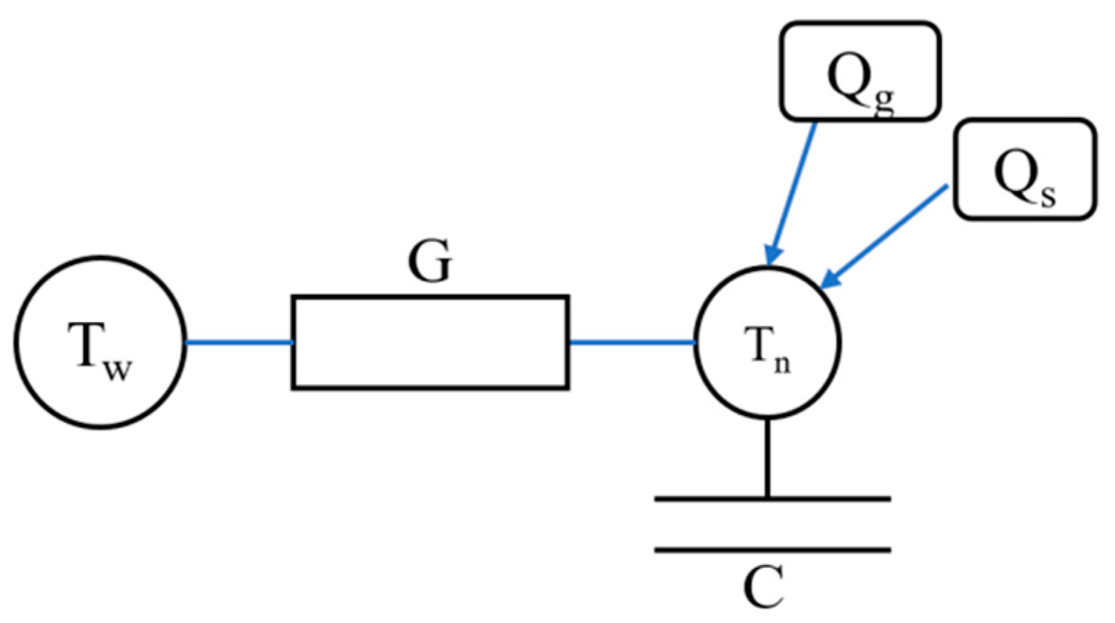
Prior to conducting the coupled simulation, an equivalent building resistance–capacitance (RC) model must first be constructed in Modelica to represent the end-user thermal load within the heating network. This approach aggregates the thermal mass of all building components that store and release heat into a single equivalent thermal capacitance, C. Similarly, the overall heat transfer resistance between the indoor environment and exterior ambient conditions through the building envelope is represented by an equivalent thermal resistance, R. Together, these parameters constitute a simplified first-order lumped-parameter RC model, as shown in Figure 1.

2.2. Coupled Secondary Network Simulation Model Integrating Modelica and EnergyPlus

2.2.1. Introduction to the Joint Simulation Module

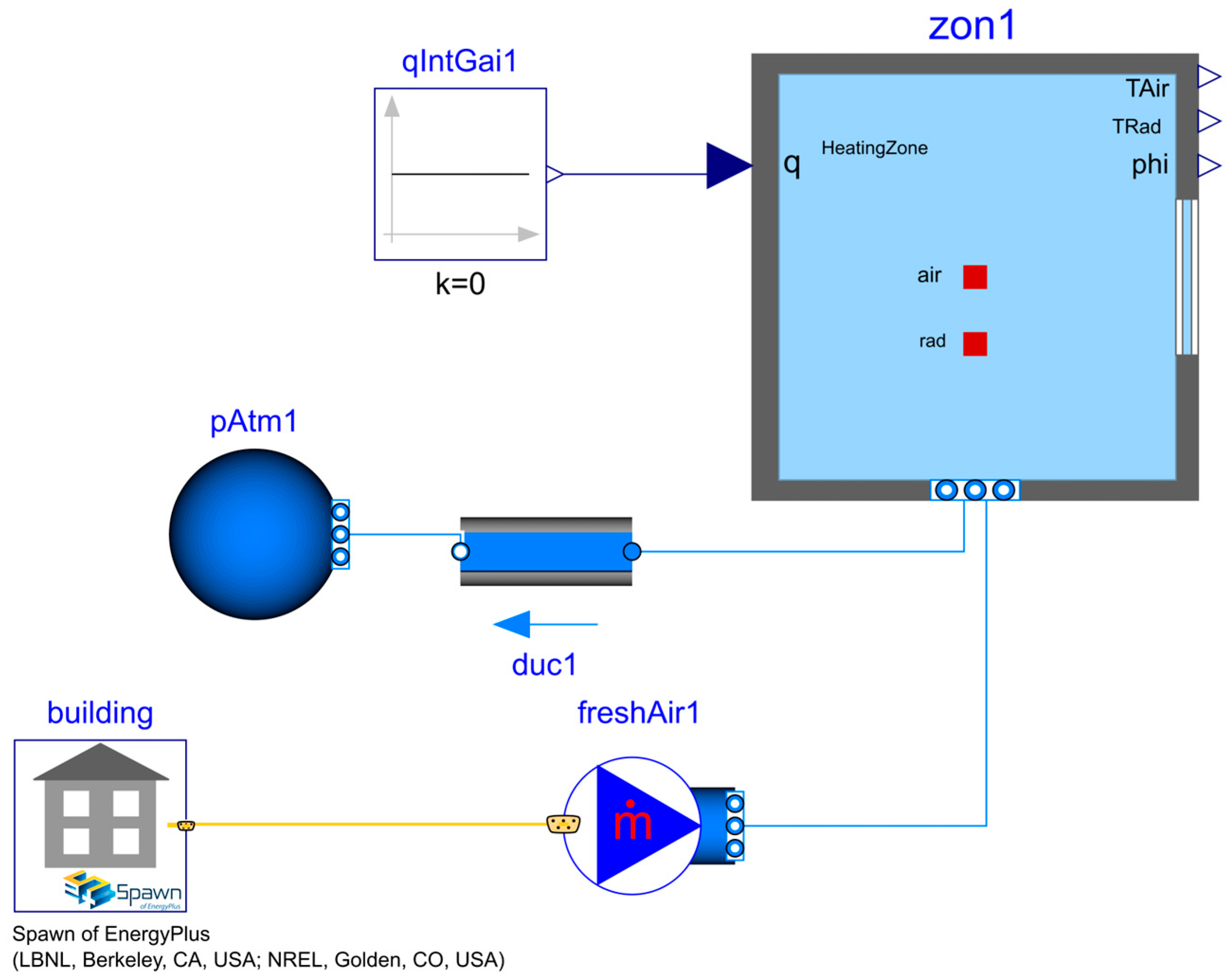
Figure 2 illustrates the system architecture of the joint simulation module, enabling a co-simulation mechanism between Modelica and EnergyPlus for the integrated thermal modeling of residential buildings. In radiant floor heating systems, the building’s thermal characteristics and the pipe network’s hydraulic properties are intrinsically coupled. Based on its high-fidelity building envelope and load calculation capabilities, this study utilizes EnergyPlus to calculate the building’s thermal load.

Within this framework, EnergyPlus executes thermal balance calculations for building zones and facilitates co-simulation with Modelica through functional mock-up units (FMUs) via the Spawn platform. Within the building module configuration, importing the predefined EnergyPlus building model and modified weather data establishes a bidirectional data exchange interface between Modelica and EnergyPlus. This coupled simulation system exhibits significant flexibility; specifically, the core ThermalZone component provides a seamless interface that supports the dynamic loading of Input Data Files (.idf) and EnergyPlus Weather Files (.epw) to accommodate the simulation requirements of diverse building types. The hybrid modeling approach utilized in this study employs a co-simulation strategy, where Modelica solves the fluid dynamics equations while EnergyPlus focuses on building thermal balance calculations.

2.2.2. Construction of District Heating Network Simulation Models

Based on the district heating system schematic, a secondary heating network model for the residential community was developed, primarily encompassing the heat exchange station, the secondary distribution network, and the comprehensive building models. To facilitate the simulation, the following strategic simplifications and assumptions were implemented:

(1) Simplifications in the Secondary Network and Station Models:

The circulating fluid within the secondary network is modeled as an incompressible liquid. Key thermophysical properties (e.g., density, specific heat) are defined as constants, thereby neglecting pressure-induced property variations.

Within the heat exchange station, thermal dissipation from internal piping and storage tanks is omitted. The modeling effort strictly isolates the water pumps and the plate heat exchanger (PHE). The PHE thermal efficiency is fixed at an empirical constant of 0.8, and transient fluctuations in the primary pump efficiency are disregarded.

Hydraulic distribution within the station is assumed to achieve steady state instantaneously. Consequently, flow rates across the secondary branches remain constant unless subjected to active flow regulation.

The pipeline topology is streamlined into a simplified trunk-and-branch configuration. Spatially adjacent consumer nodes exhibiting similar thermal load profiles are aggregated.

(2) Simplifications in the EnergyPlus Building Models:

Architectural geometries are streamlined: irregular structural protrusions are approximated as rectangular volumes, strictly constraining the geometric deviation to within 5%.

Micro-scale thermal bridges (e.g., windowsills, structural overhangs) are excluded from the heat transfer calculations, and window fenestrations are geometrically simplified.

Slight gradients on floors and roofs, which serve solely for drainage, are mathematically flattened.

Adhering to standard residential occupancy profiles, internal thermal gains generated by appliances, lighting, and occupants are prescribed via deterministic time-series schedules, neutralizing stochastic inter-room behavioral discrepancies.

(3) Establishment of System Boundary Conditions:

To guarantee the fidelity and engineering pragmatism of the source-network-load co-simulation framework, rigorous boundary conditions were calibrated against empirical operational data:

Meteorological boundaries: Ambient environmental inputs are driven by empirical hourly weather data (e.g., outdoor dry-bulb temperature) recorded in the target locale during the 2023–2024 heating season, ensuring the authentic replication of dynamic outdoor thermal disturbances.

Hydraulic boundaries: The primary network’s hydraulic parameters are rigorously benchmarked against municipal operational logs. Within the Modelica environment, a Boundary_pT component is deployed on the return locus to anchor the system’s static pressure at a constant 1.0 MPa. Concurrently, the operational pressure at the thermal inlet is maintained at 1.0 MPa. Acknowledging that the actual primary return pressure oscillates between 400 and 500 kPa, the simulation conservatively adopts an equivalent steady state of 500 kPa. This regularization is critical for ensuring the numerical convergence and representativeness of the hydraulic solver.

Thermal and physical boundaries: The transient thermal dynamics of the building envelopes are evaluated via a reduced-order RC model, whose nodal parameters are strictly synthesized from the inherent thermophysical properties of the actual construction materials. Moreover, to rigorously quantify conductive heat losses along the distribution routing, the thermal conductivity of the pipe insulation is locked at an empirical engineering standard of 0.033 W/(m·K).

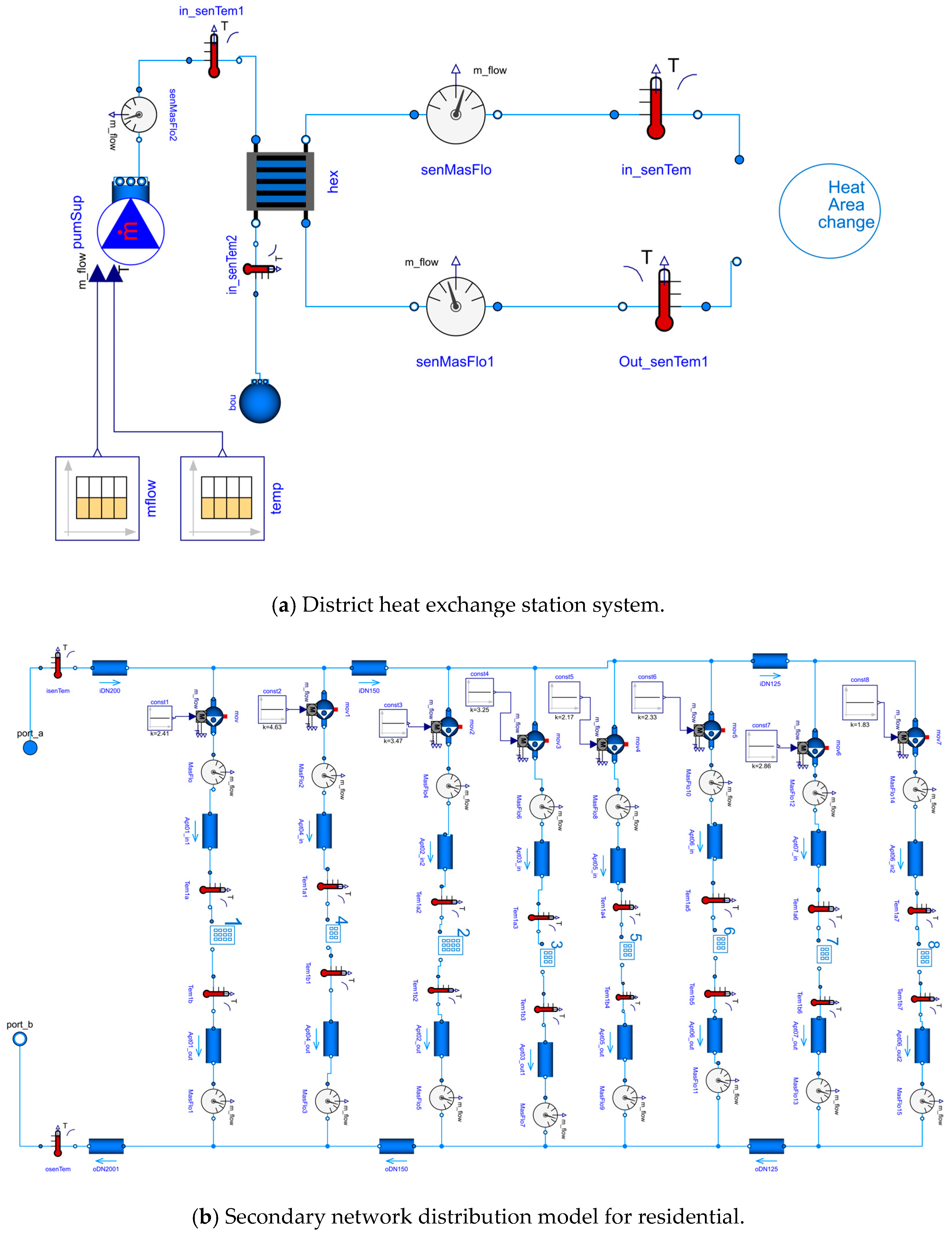
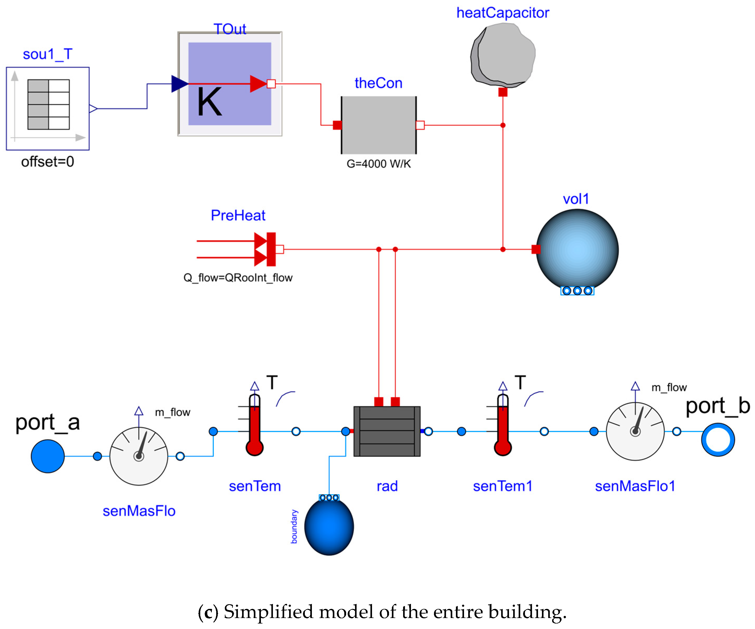
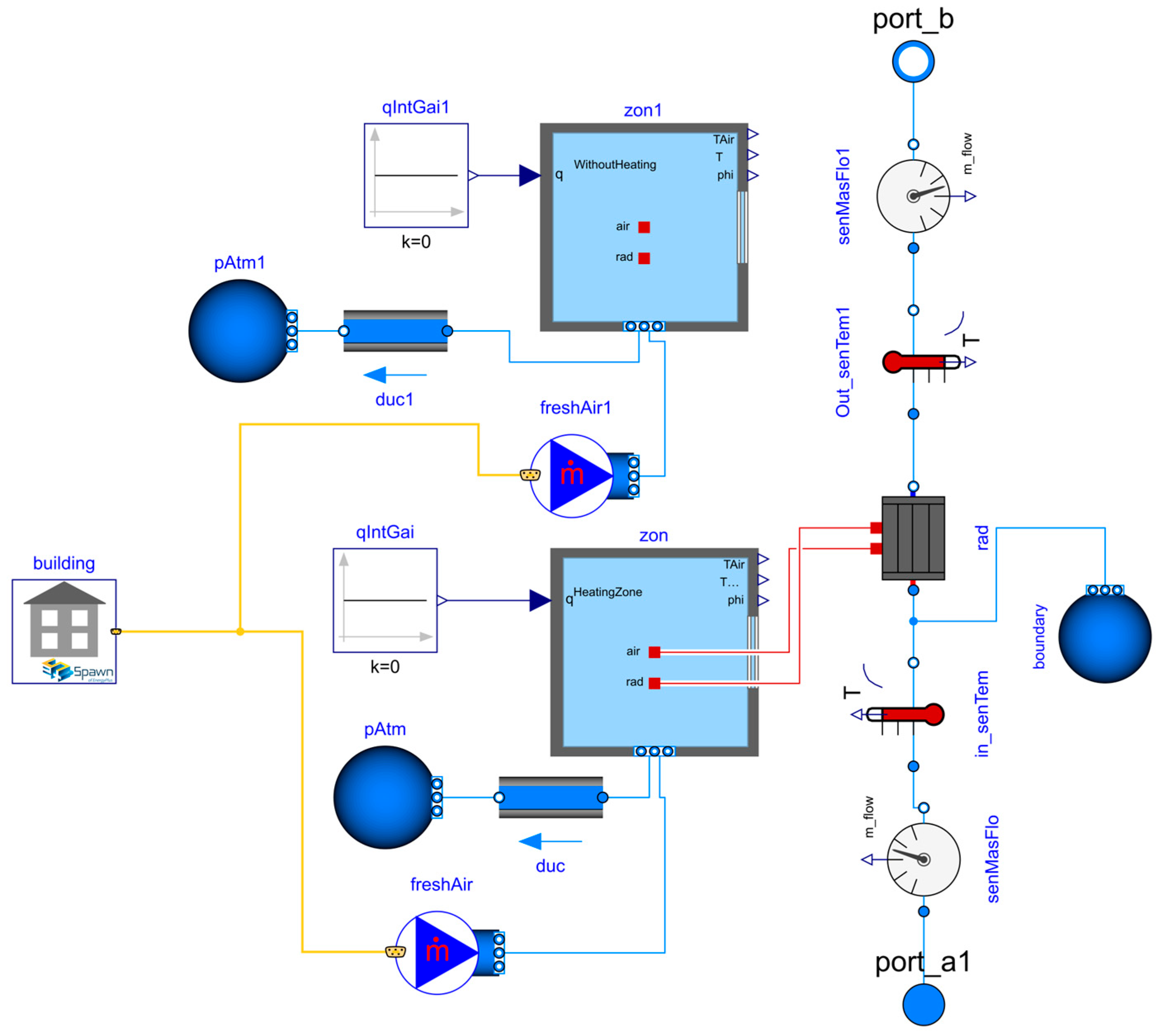
Synthesizing these simplifications, operational assumptions, and boundary configurations, the foundational source-network-load physical model was successfully formulated, as depicted in Figure 3a–c.

Figure 3a depicts the developed heating system model. Primary network supply conditions, including flow rate and temperature, are defined as inputs that regulate the secondary network through plate heat exchangers, representing the core regulatory logic of the system. As the system connects to the municipal pipe network, the primary return flow directly interfaces with the Boundary_pT source model. This component provides a highly configurable fluid boundary condition suitable for simulating systems that require the precise control of fluid pressure, temperature, and medium composition.

Figure 3b presents the integrated secondary network model architecture. According to field operational data, flow rates within the secondary pipelines remained nearly constant during the heating season, exhibiting minimal fluctuations of approximately ±0.01 kg/s. Consequently, the flow control for each branch is achieved by implementing individual pump models.

Figure 3c depicts a simplified building model coupled to a radiant heating unit. By providing both convective and radiant heat, this configuration represents the user-side terminal of the comprehensive heating system. This configuration serves as a simplified load to validate the accuracy of the overall district heating network model.

As several residential units remained unheated during the observation period, it is necessary to refine the thermal zone segmentation based on actual occupancy and operational conditions. To this end, this study employs a zoned thermal balance modeling approach to accurately reflect the dynamic thermal behavior of varying thermal zones.

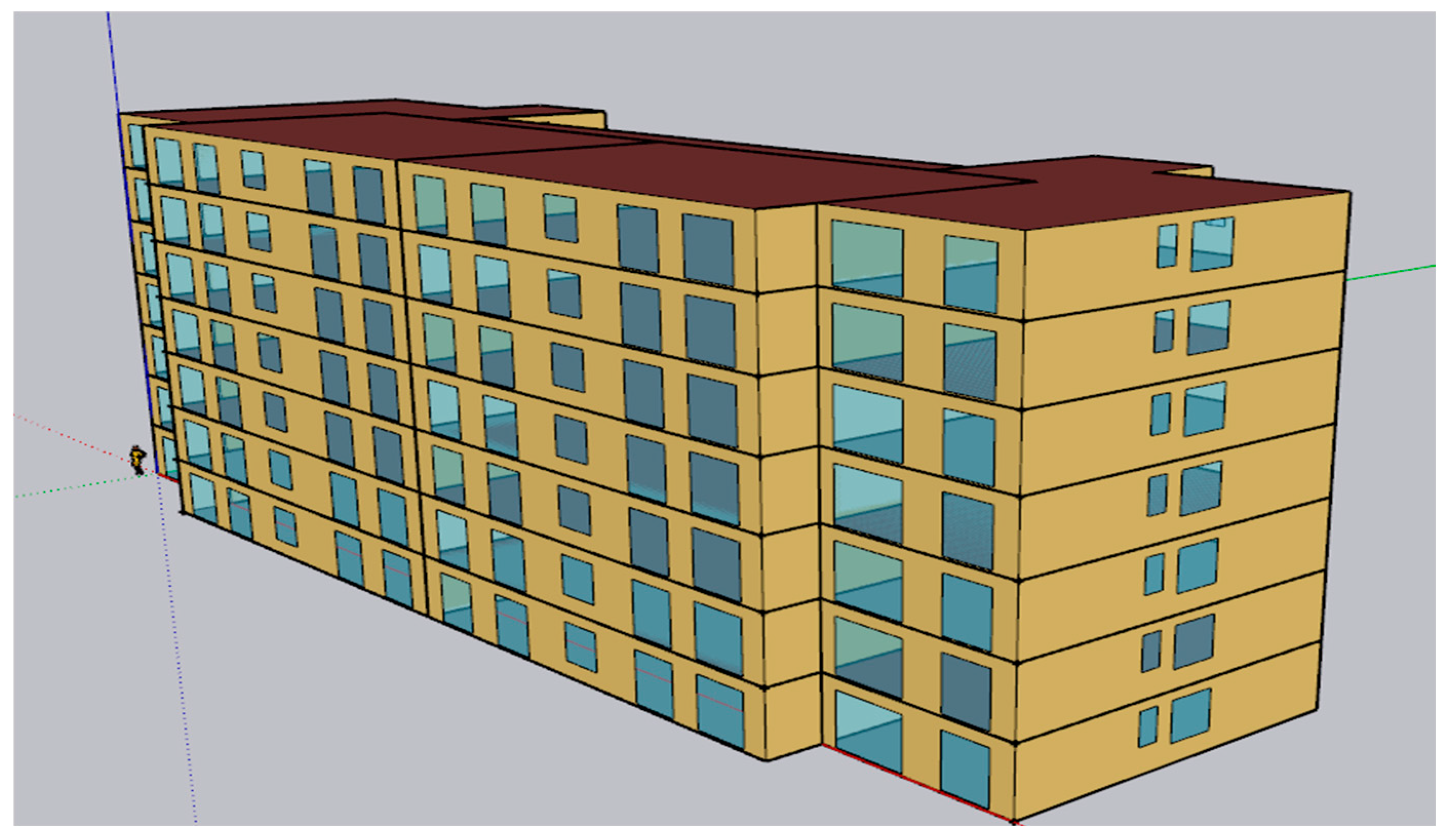
Building 4, as a typical seven story residential building, has a three-dimensional physical model as shown in Figure 4. It has been selected as a representative case for this study, and the system configuration is detailed in Figure 5. The selection of this building is justified by its high degree of typicality and prevalence within the district in terms of architectural layout, occupancy patterns, and thermal envelope characteristics. Furthermore, the precise physical properties of the building envelope are rigorously configured based on actual engineering design data, with detailed parameters provided in

Table 1. Design values of heat transfer coefficients for building envelope structures.

Enclosure Structure Section	Design Value of Heat Transfer Coefficient W/(m2·K)
Roof	0.36
Exterior wall	0.44
Floor	0.56
Partition wall separating heating and non-heating spaces	0.90
Door separating heating and non-heating spaces	1.70
Exterior window	3.40

.

The thermal zones are categorized as follows:

Thermal Zone 1 (heated units) represents the active heating area, coupled with the district heating network model to simulate operational heating conditions.

Thermal Zone 2 (unheated units) accounts for non-heated residential spaces, considering only the thermal mass of the building structure and ambient heat exchange.

In subsequent simulations, should detailed analysis of individual rooms be required, the zoning granularity can be increased to achieve high-fidelity thermal environment modeling. This approach significantly improves the precision of building thermal models while providing a reliable computational framework for evaluating the impact of various heating strategies on overall energy consumption.

2.3. White-Box Model Control Strategy

2.3.1. Model Predictive Control Strategy Development

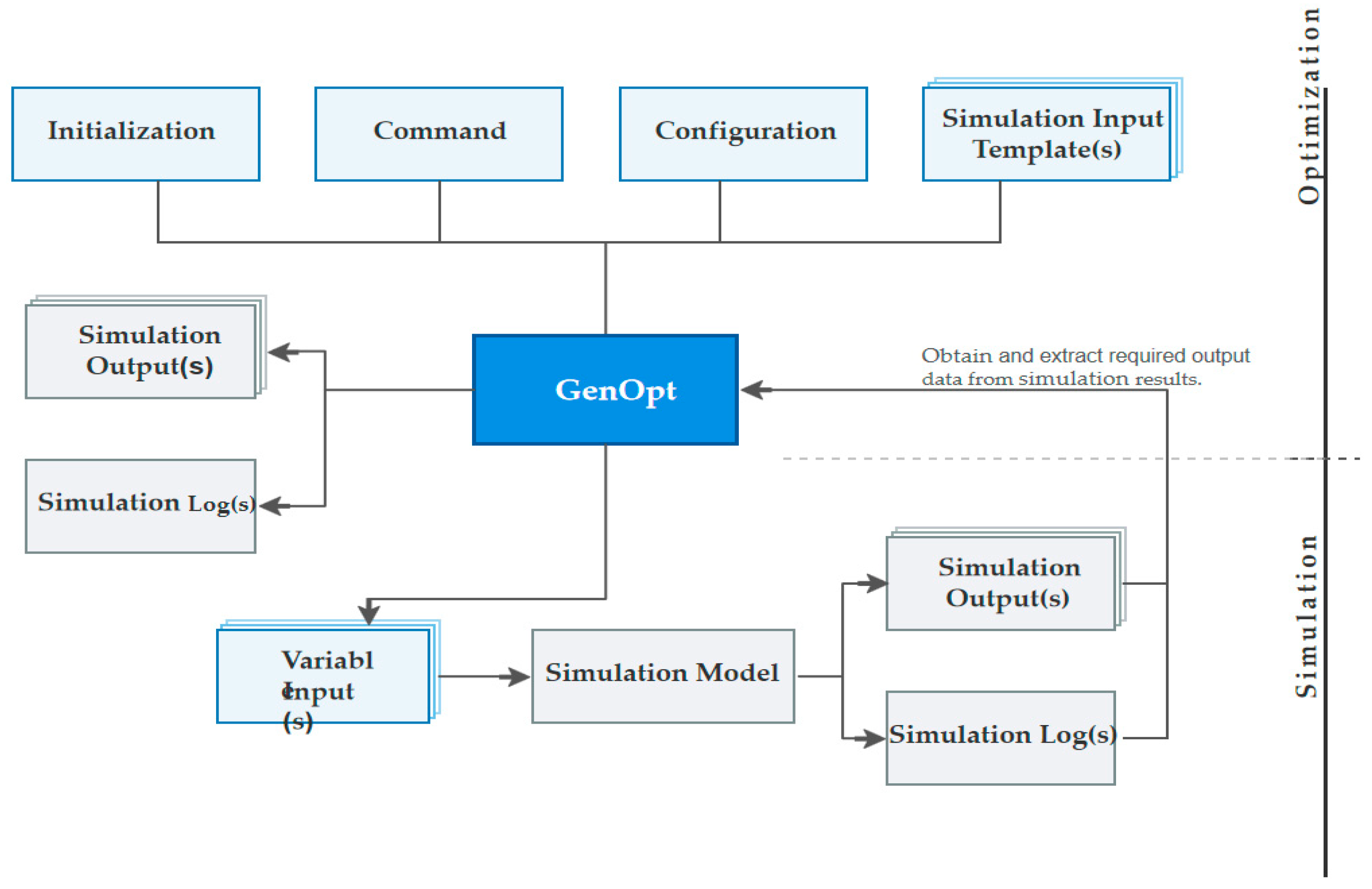
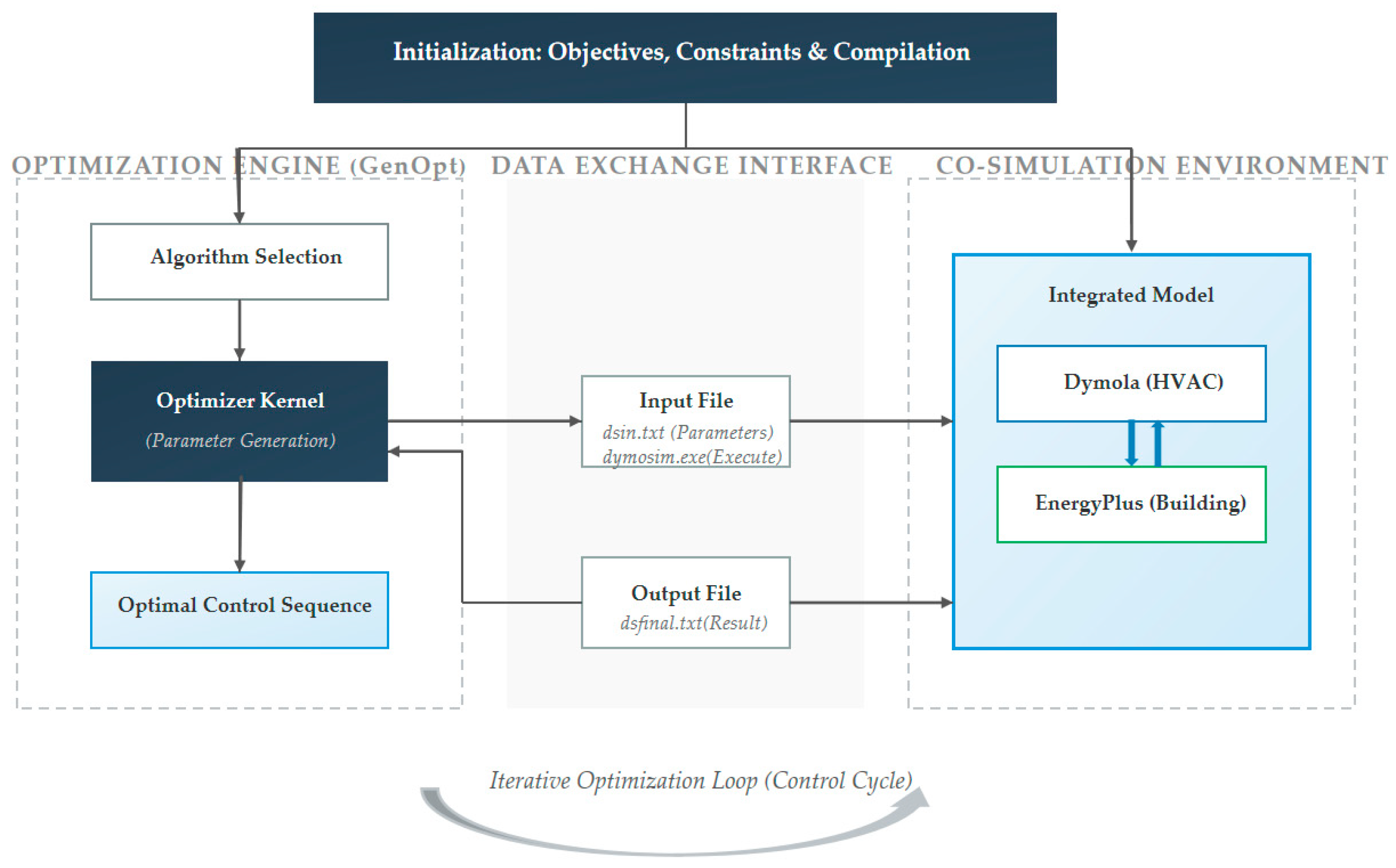
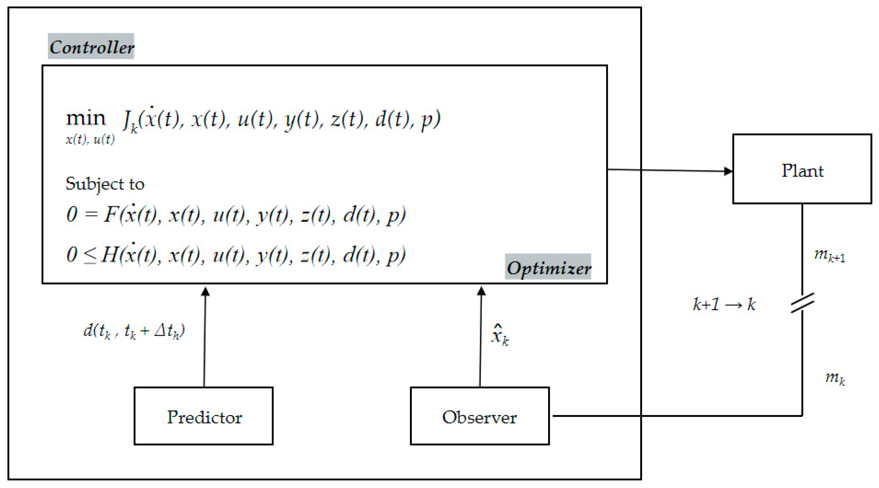
This study develops an MPC architecture for the heating system by integrating a Dymola white-box model with GenOpt 3.1.1 optimization software. The resulting architecture comprises two functional levels: an optimization layer and a simulation layer. The optimization layer orchestrates GenOpt to invoke Dymola for co-simulation and iterative optimization, thereby generating optimal operating sequences. The simulation layer represents the actual execution process, validating the control results produced by the optimization layer. The framework is illustrated in Figure 6 and Figure 7.

The design of the objective function primarily revolves around several key factors: indoor comfort, energy savings, and system stability [45].

(1) Thermal comfort objective

Minimization of the setpoint tracking error: This objective seeks to minimize the Mean Squared Error (MSE) between the dynamic indoor temperature and the prescribed thermal setpoint $T_{\mathit{set}}\left(k\right)$. In this context, k represents the discrete time index within the prediction horizon, designating the k-th future sampling step relative to the current control interval $T_{room}(k)$.

$$J_{\mathit{comfort}}={\displaystyle \frac{1}{24}}{\displaystyle \sum _{k=1}^{24}{\left(T_{\mathit{room}}\left(k\right)-T_{\mathit{set}}\left(k\right)\right)}^2}$$

(11)

where the prescribed thermal setpoint $T_{set}$ is established at 18 °C during daytime hours and 22 °C during the nighttime. In this study, both the prediction horizon $N_p$ and the control horizon $N_c$ are configured to 24 time steps (equivalent to a 24 h timeframe, i.e., $N_p$ = $N_c$ = 24). This horizon length is strategically selected to encompass a full diurnal heating cycle, thereby effectively accommodating the substantial thermal propagation delay inherent within the district heating network.

(2) Energy conservation objective

Penalization of control effort: This objective minimizes the total heat delivered to the system by quantifying the energy consumption through thermal power calculations $Q=G\cdot \rho \cdot c_p\cdot \Delta T$.

$$J_{\mathit{energy}}={\displaystyle \sum _{k=1}^{N_p}\alpha \cdot G\left(k\right)\cdot \left(T_{\mathit{supply}}\left(k\right)-T_{\mathit{return}}\left(k\right)\right)}$$

(12)

where $G(k)$ designates the control input (i.e., the mass flow rate); $\alpha$ is the prescribed weighting penalty factor for the control input; $T_{supply}(k)$ represents the supply temperature of the secondary network; and $T_{return}(k)$ corresponds to the return temperature of the secondary network.

(3) System stability objective

Penalization of control increments: This objective limits the rate of change in the manipulated variables to prevent premature actuator (valve) wear induced by high-frequency modulations, and to avert excessive supply–return temperature differentials within the secondary network.

$$J_{smooth}={\displaystyle \sum _{k=1}^{N_p}\left(\beta \cdot {\left(G(k)-G(k-1)\right)}^2+\gamma \cdot {(T_{supply}(k)-T_{return}(k)-\Delta T_{max})}^2\right)}$$

(13)

where $\Delta T_{max}$ designates the maximum allowable temperature difference between the supply and return water; $\beta$ is the assigned weighting penalty coefficient for the input flow variations, taking a value of 0.7; and $\gamma$ represents the penalty coefficient for the temperature fluctuations, set to 0.3.

$$J_{smooth,1}={\displaystyle \sum _{k=1}^{N_p}\left|T_{supply}(k)-T_{return}(k)-\Delta T_{max}\right|}$$

(14)

(4) Comprehensive objective function for the quality regulation strategy

$$J={\omega }_{comfort}{J}_{comfort}+{\omega }_{smooth}{J}_{smooth,1}$$

(15)

where ${\omega }_{comfort}$ denotes the weighting coefficient for thermal comfort, specified as 0.6; and ${\omega }_{smooth}$ represents the weighting coefficient for operational stability, specified as 0.4. Given the service-oriented nature of district heating operations, a higher priority (weight) is strategically allocated to the comfort objective to preempt potential user complaints stemming from inadequate thermal satisfaction.

Input constraints:

$$T_{supply,min}\le T_{supply}(k)\le T_{supply,max}$$

(16)

where $T_{set,\min }$ = 36 °C; and $T_{set,\max }$ = 52 °C.

Output constraints:

$$T_{set,\min }-\Delta T\le T_{room}(k)\le T_{set,\max }+\Delta T$$

(17)

where $T_{set,\min }$ = 18 °C; $T_{set,\max }$ = 22 °C; and the tolerance band $\Delta T$ = 1 °C. This configuration establishes a thermal deadband, permitting the indoor temperature to safely fluctuate within a predefined tolerance threshold.

(5) Comprehensive objective function for the quality and quantity regulation strategy

$$J=J_{comfort}+J_{energy}+J_{smooth}$$

(18)

Input constraints:

To guarantee that the flow regulation (quantity regulation) satisfies the thermal load requirements, its maximum regulative capacity is explicitly quantified. Once the actual load demand surpasses the operational limits of this quantity regulation, quality regulation is subsequently triggered to execute necessary heat supplementation or curtailment. Consequently, the coupled constraints governing the flow rate and thermal load are established as follows:

$$G(k)={\displaystyle \frac{Q(k)}{c\cdot \rho \cdot (T_{\mathrm{supply}}-T_{\mathrm{return}})}}$$

(19)

where $Q(k)$ denotes the nominal thermal load; $\Delta T_{\max }$ represents the thermal propagation delay of the heating network; $Q_{\max }$ specifies the baseline supply temperature, configured at 42 °C; and $\Delta T_{\min }$ corresponds to the return temperature, established at 37 °C.

$$G_{\min }\le G(k)\le G_{\max }$$

(20)

$$G_{\min }={\displaystyle \frac{Q_{\min }(k+{\tau }_{\mathrm{model}})}{c\cdot \rho \cdot \Delta T_{\max }}}$$

(21)

$$G_{\max }={\displaystyle \frac{Q_{\max }(k+{\tau }_{\mathrm{model}})}{c\cdot \rho \cdot \Delta T_{\min }}}$$

(22)

where $Q_{\min }$ denotes the minimum thermal load across the entire heating season; $\Delta T_{\max }$ represents the maximum supply–return temperature differential; $Q_{\max }$ designates the peak thermal load during the heating season; and $\Delta T_{\min }$ corresponds to the minimum supply–return temperature differential.

To prevent abrupt hydraulic fluctuations, a rate-of-change constraint is imposed on the mass flow rate. This limits regulative volatility and safeguards the stability of the indoor thermal environment:

$$\left|G(k)-G(k-1)\right|\le G_{\max }$$

(23)

Output constraints:

$$T_{set,\min }-\Delta T\le T_{room}(k)\le T_{set,\max }+\Delta T$$

(24)

where $T_{set,\min }$ = 18 °C; $T_{set,\max }$ = 22 °C; and the tolerance band $\Delta T$ = 1 °C. This establishes a thermal deadband, permitting the indoor temperature to safely fluctuate within a permissible tolerance.

To curb energy consumption without compromising thermal comfort, an operational constraint is imposed on the water pump. Crucially, to prevent the sacrifice of comfort for energy savings, this constraint is conditionally activated only when the pump’s energy consumption exceeds the nominal baseline by 20%:

$$W_{\mathrm{pump}}(k)\le 1.2\cdot W_{\mathrm{pump},\mathrm{base}}(k)$$

(25)

$$W_{\mathrm{pump},\mathrm{base}}(k)={\displaystyle \frac{\rho gH{G}_{\min }}{{\eta }_{\mathrm{pump}}}}$$

(26)

where $W_{\mathrm{pump},\mathrm{base}}(k)$ denotes the baseline pump energy consumption commensurate with the thermal load, and ${\eta }_{\mathrm{pump}}$ represents the pump efficiency, designated as 92.6%.

System dynamic constraints:

$$x\left(k+1\right)=f\left(x\left(k\right),u\left(k\right),d\left(k\right)\right)$$

(27)

where $x\left(k\right),u\left(k\right),d\left(k\right)$ designate the state vector, output vector, and disturbance vector, respectively. The disturbance vector $d\left(k\right)$ encompasses the outdoor air temperature and internal heat gains. For the outdoor meteorological parameters, the system interfaces with external weather forecasting services to acquire hourly predictive data over the future prediction horizon (e.g., the ensuing 24 h). Regarding the internal heat gains, given the inherent regularity of residential occupancy, these are rationally estimated using standardized hourly profiles derived from historical statistical data and normative building codes.

This study employs the particle swarm optimization (PSO) algorithm within GenOpt to optimize and solve white-box model predictive control (MPC). The relevant expressions are as follows:

$$\left\{\begin{array}{l}{v}_i(t+1)=\omega v_i(t)+c_1{r}_1[p_i(t)-x_i(t)]+c_2{r}_2[g(t)-x_i(t)]\\ x_i(t+1)=x_i(t)+v_i(t+1)\end{array}\right.$$

(28)

where $v_i\left(t\right)$p_i(t) is the historical optimal position for particle i; $p_i(t)$ on; $\omega$ is the inertial weighting; $c_1$ is the individual learning factor, also known as individual acceleration factor; $c_2$ is the social learning factor, also known as the social acceleration factor; $r_1$, $r_2$~U(0,1)—0–~1 is 0–~1 random disturbance terms uniformly distributed between 0~1; $x_i(t)$, $v_i(t)$—are the position state and velocity vector of each particle at time t.

Furthermore, the established MPC framework rigorously operates on the receding horizon principle. This study strategically couples implicit MPC with a direct transcription method, establishing the MPC as a model-based, closed-loop optimization strategy over a finite horizon. Within each optimization cycle, the controller computes the optimal control sequence across the entire prediction horizon based on the most recent measured states. As the system transitions to the subsequent time step, the prediction horizon shifts forward; the algorithm incorporates the latest empirical measurements to update the initial state and subsequently re-solves the optimization problem. This receding-loop feedback mechanism inherently compensates for deviations induced by model simplifications, unmeasured disturbances, and meteorological forecast inaccuracies, thereby substantially bolstering the system’s robustness.

During the execution of the MPC algorithm, each discrete time step j plays a pivotal role. Initially, utilizing the measurement vector m_k, the system deploys an observer to precisely estimate the state vector, which comprehensively encapsulates the current dynamic state of the controller model F. Subsequently, leveraging the explicit formulation of model F alongside a predefined objective function J, the algorithm optimizes the future trajectories of the system states x and control inputs u across the finite prediction horizon. Crucially, this optimization is not unconstrained; rather, it is strictly bounded by a predefined constraint set H. It is worth noting that the construction and evaluation of J, F, and H are fundamentally governed by multiple interrelated variables, including model outputs y, algebraic variables z, exogenous disturbances d, and system parameters p. Furthermore, predictive disturbance data over the horizon, supplied by the forecasting module, are integrated as exogenous inputs to guide the optimization process. The objective function J is conventionally formulated via the integration of relevant model variables over the prediction horizon, mathematically expressed as follows:

$$J_k={\displaystyle {\int }_{(t=tk)}^{(tk+\Delta th)}l\left(\widehat{x}\left(t\right),x\left(t\right),u\left(t\right),z\left(t\right),d\left(t\right),p\right)dt}$$

(29)

The detailed algorithmic flowchart is illustrated in Figure 8.

2.3.2. MPC Quality Regulation Control Strategy

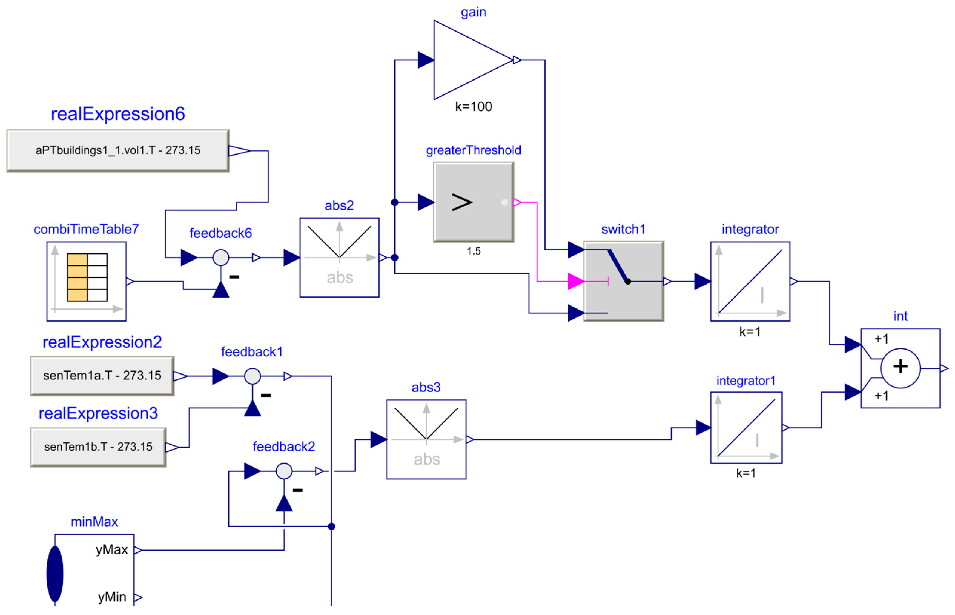
As shown in Figure 9, Field tests characterizing network delays reveal that the source-network-load heating system exhibits a thermal lag of 1.5 to 2 h. This delay occurs when regulating the secondary network supply temperature via adjustments to the primary-side hot water flow rate. To account for this phenomenon, a lag parameter is integrated into the Modelica pipe model to accurately simulate the thermal delay characteristics of the distribution network. Under this operational scenario, the secondary network supply water temperature serves as the primary optimization target. Given that the secondary network flow rate remains constant under this condition, an objective function module was developed in Dymola incorporating the comfort and stability modes detailed in Section 2.3.1.

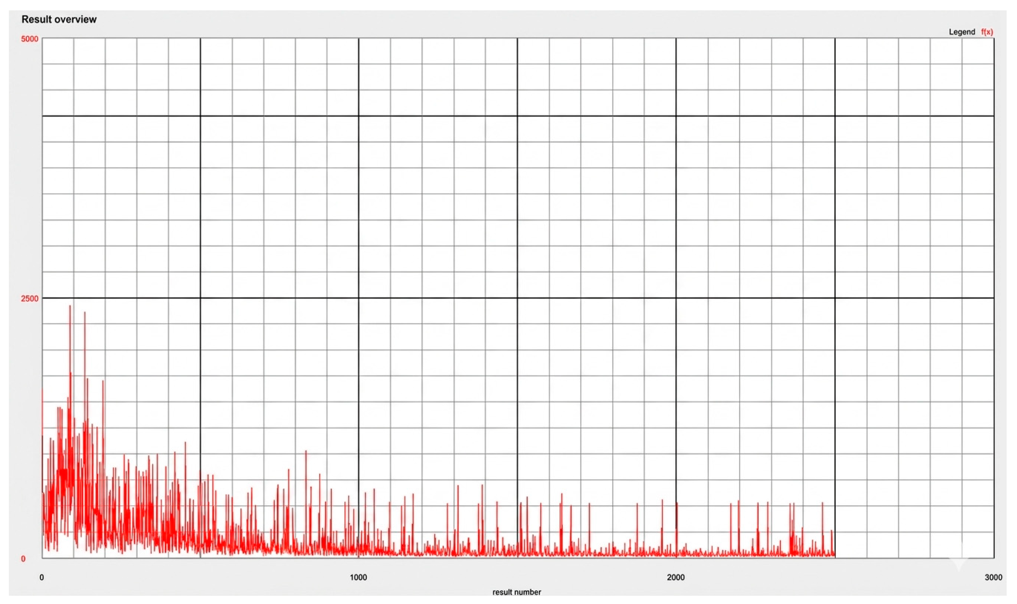
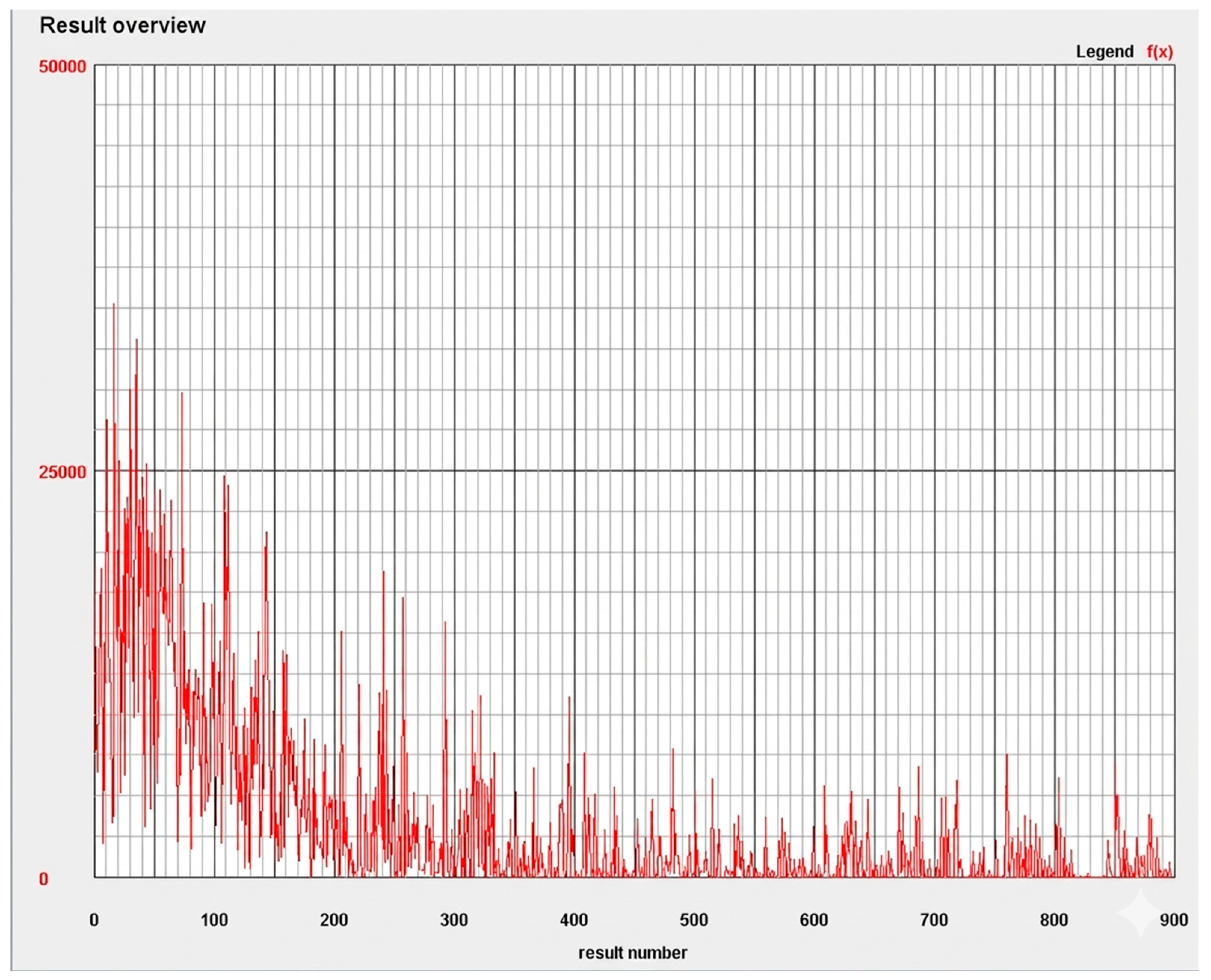
The Figure 10 above illustrates the convergence trajectory of the GenOpt-based objective function, with the vertical axis representing the objective function value and the horizontal axis indicating iteration counts. The results exhibit a consistent reduction in the objective function value as the iterations progress, indicating a successful minimization process. The final optimal control sequence corresponds to the parameter set achieved when the objective function converges to its minimum value.

2.3.3. MPC Quality and Quantity Regulation Control Strategy

In the investigated system, each user terminal is equipped with a flow control valve, facilitating decentralized flow regulation. Within centralized heating operation strategies, quantity regulation (flow control) offers significant energy-saving advantages and adaptability compared to traditional quality regulation (temperature control); however, it is susceptible to hydraulic imbalance [46]. Research indicates that staged variable-flow regulation achieves superior energy savings relative to constant-flow mass control. Furthermore, quality–quantity parallel control simultaneously reduces thermal and electrical energy consumption while providing the flexibility required for optimal system operation [29,47]. This study designs a quality–quantity parallel regulation MPC control strategy to further improve the heating system. To prevent hydraulic imbalance, the valve opening variation range is constrained in the MPC system design to mitigate local overpressure or underpressure issues.

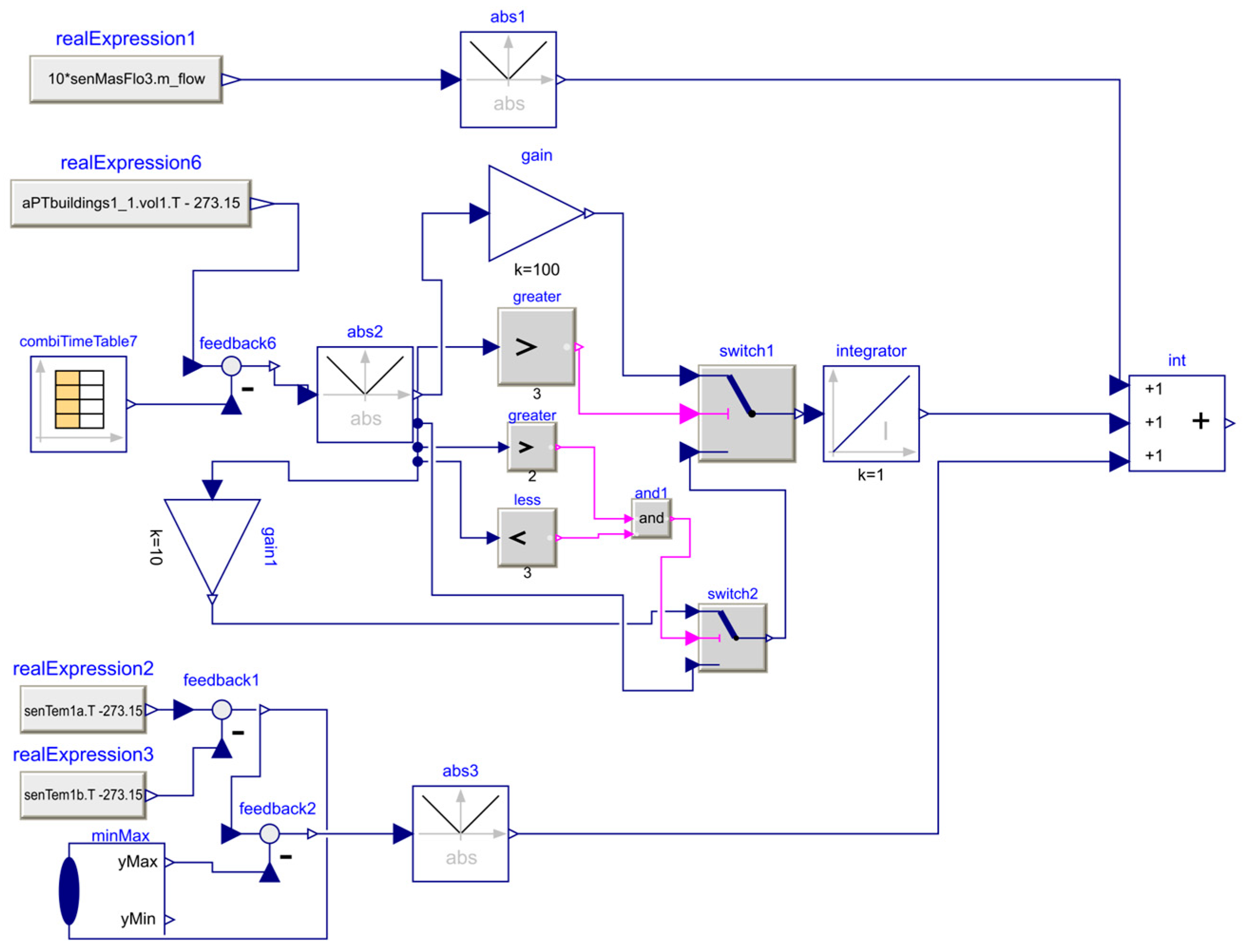
As shown in Figure 11, This study develops a quality-and-quantity parallel MPC strategy to enhance the overall performance of the heating system. To preclude hydraulic imbalance, valve opening ranges are constrained within the MPC framework to mitigate local pressure fluctuations. Under this operational scenario, the secondary network supply water temperature and the supply flow rate for Building 1 are selected as dual optimization targets. By integrating the energy-saving, comfort-oriented, and stability-oriented criteria described in Section 2.3.1, a multi-objective function module was implemented in Dymola.

Figure 12 illustrates the convergence process of the GenOpt optimization objective function, with the vertical axis representing the objective function value and the horizontal axis indicating iteration counts. The high number of iterations in this optimization process demonstrates a significant decrease in the objective function value as iterations progress, followed by a minor fluctuation. The optimization result corresponding to the lowest objective function value is presented as the control sequence.

3. Case Study

3.1. Actual Project Introduction

To evaluate the performance, robustness, and generalizability of the proposed MPC method, the model was validated using a real-world engineering case study. The case study focuses on the heating renovation project of the Xuanyuan Huafu residential community in Xinzheng City, covering a total heated floor area of 46,281 m². By renovating the secondary heating network, residential pipeline wells, and public area heating systems, the project attained enhanced operational flexibility. Indoor terminals utilize low-temperature radiant floor heating, while the district heat exchange station operates with a design supply/return temperature of 45/35 °C. The proposed control strategies across various operating conditions were validated primarily using Building 1 as the representative model.

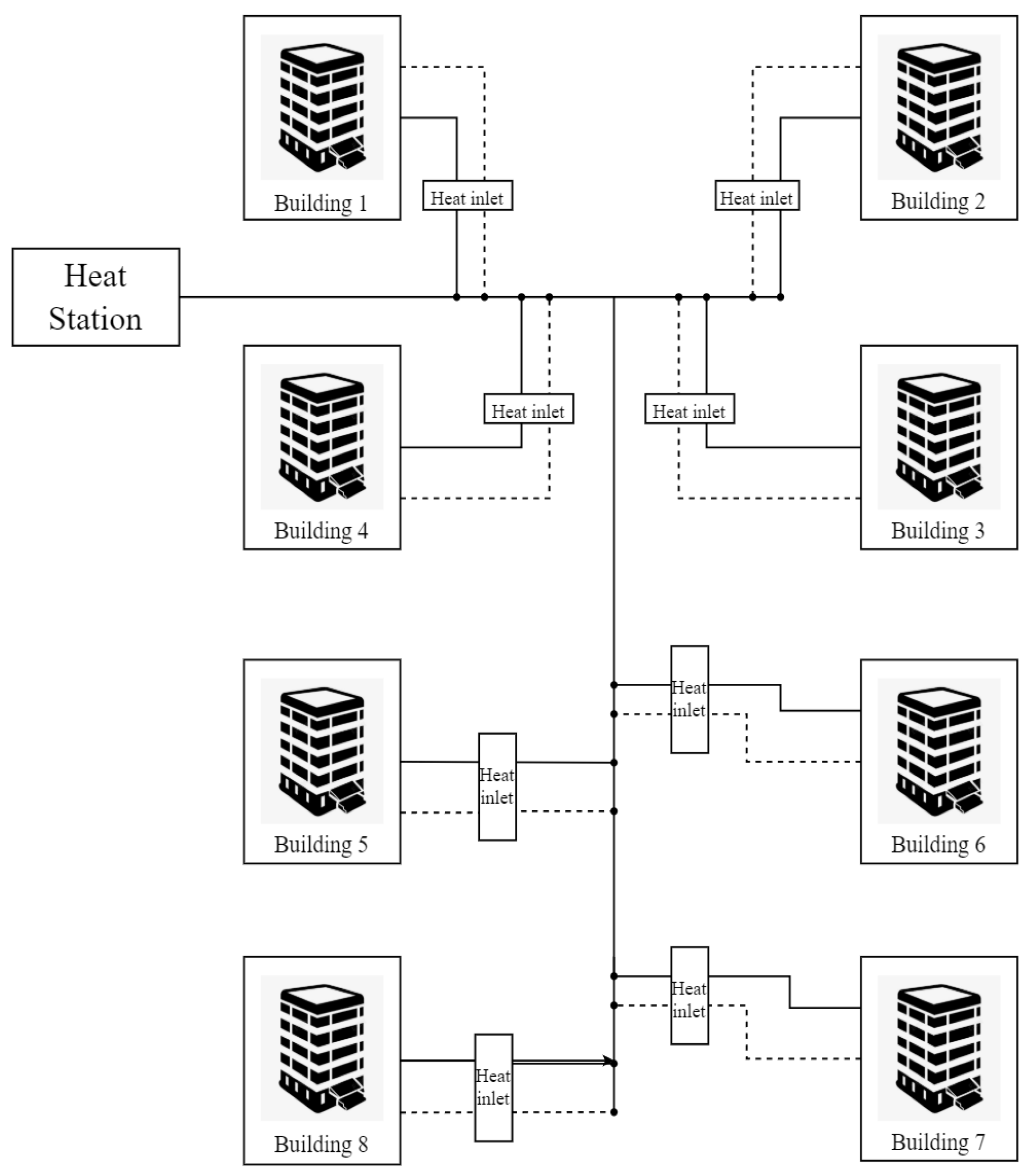
Figure 13 illustrates the heating process flow diagram, showing the pipe network branching into two main headers from the heat exchange station to supply the individual residential buildings.

3.2. Calibration of System Coupled Simulation Models Based on Operational Data

To ensure the practical applicability of the proposed model in real-world engineering projects, systematic calibration based on measured field data is essential. This study utilizes GenOpt to perform automated calibration, aiming to minimize the Normalized Mean Biased Error (NMBE) between simulated and measured values. The calibration objective function is expressed as follows:

$$J_{cab}=\min (NMBE)=\min \left({\displaystyle \frac{{\displaystyle \sum _{i=1}^N|S(i)-M(i)|}}{{\displaystyle \sum _{i=1}^{N}M(i)}}}\right)$$

(30)

where S(i) is the simulated calculation value for the i-th data point or time step; M(i) is the experimental measurement value for the i-th data point or time step; N is the total number of discrete data points or time steps within the corresponding time period.

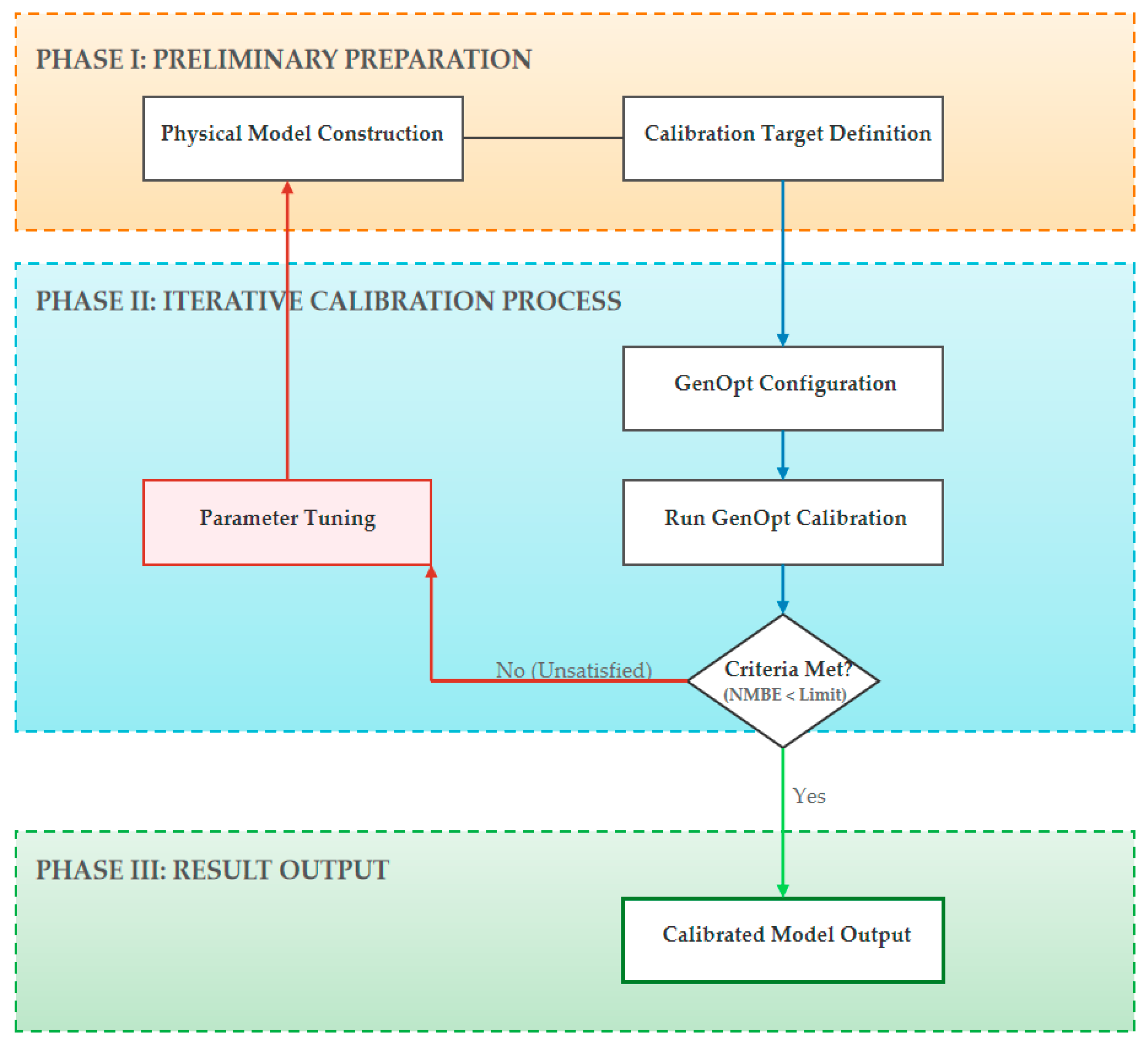
The model calibration process based on joint simulation optimization is shown in Figure 14.

This iterative process leverages empirical data as dynamic boundary conditions, continuously inputting them into the Modelica model to execute simulations and compute the Normalized Mean Bias Error (NMBE). Functioning as the overarching optimization engine, GenOpt evaluates these outputs and deploys an optimization algorithm to iteratively fine-tune the model parameters until the NMBE between the simulated responses and the empirical measurements is rigorously minimized. The primary parameter range for this calibration encompasses the mass flow rate setpoints or the supply/return temperature setpoints. Notably, the calibration protocol utilizes actual operational heating data—specifically, the indoor thermal profiles of the end-users—to optimize the flow rate of the primary network. Convergence of the optimization process is achieved when the differential change in the decision variables or the algorithmic search step size shrinks below a predefined tolerance threshold. The comprehensive calibration results are subsequently detailed in Section 4.2.

3.3. MPC Operating Conditions

As shown in

Table 2. Flow control valve for Building 1.

Time	Flow Rate (kg/s)	Flow Rate (m3/h)
1:00	0.31	1.12
2:00	1.19	4.28
3:00	0.31	1.12
4:00	0.31	1.12
5:00	1.22	4.39
6:00	1.28	4.61
7:00	0.31	1.12
8:00	0.31	1.12
9:00	1.22	4.39
10:00	1.00	3.60
11:00	1.25	4.50
12:00	1.25	4.50
13:00	0.31	1.12
14:00	1.00	3.60
15:00	1.25	4.50
16:00	1.22	4.39
17:00	0.31	1.12
18:00	1.22	4.39
19:00	1.28	4.61
20:00	1.19	4.28
21:00	1.25	4.50
22:00	1.28	4.61
23:00	0.31	1.12

, MPC Case Study A: On 24 January 2025, the indoor temperature of Unit 2-1602 in Building 1 was designated as the primary control target. Supply flow rates within Building 1 were dynamically modulated via terminal electric control valves. The model predictive control strategy was implemented utilizing the co-simulation framework of Dymola and EnergyPlus (EP). The setpoint temperature for Building 1 was established at 22 °C. Using this setpoint as the control objective, the system’s hydraulic adjustment range was evaluated. Based on on-site operational data, the permissible flow adjustment range was determined. The hourly mass flow rates for Unit 2 were defined as the vector {0.31, 1.19, 1.22, 1.25, 1.28} (kg/s). This optimized control sequence was applied to the heating system serving the residential units in Unit 2 of Building 1.

As shown in

Table 3. Secondary network temperature regulation chart.

Time	Secondary Network Supply Water Temperature Setting (K)	Secondary Network Supply Water Temperature Setting (°C)
1:00	313.15	40
2:00	315.15	42
3:00	312.15	39
4:00	309.15	36
5:00	314.15	41
6:00	309.15	36
7:00	313.15	40
8:00	311.15	38
9:00	312.15	39
10:00	311.15	38
11:00	313.15	40
12:00	311.15	38
13:00	309.15	36
14:00	309.15	36
15:00	315.15	42
16:00	309.15	36
17:00	312.15	39
18:00	314.15	41
19:00	317.15	44
20:00	317.15	44
21:00	312.15	39
22:00	309.15	36
23:00	309.15	36

, MPC Case Study B: On 25 January 2025, the secondary network supply temperature setpoint was modulated, with the indoor temperature of Building 1 serving as the control target. The model predictive control strategy was implemented utilizing the co-simulation framework of Dymola and EnergyPlus. The target indoor temperature for Building 1 was established at 22 °C. To achieve this target, the secondary network temperature followed a setpoint trajectory of {42, 41, 40, 39, 38, 37, 36} (°C), representing the supply temperature at each discrete time step. This control scheme facilitated the precise regulation of the heating system for the residential units within Building 1.

4. Results and Discussion

4.1. Model Evaluation

To quantify the predictive accuracy of the proposed model, this study employs four statistical metrics: Mean Squared Error (MSE), Root Mean Squared Error (RMSE), Mean Absolute Error (MAE), and Relative Mean Deviation (RMD). The calculation of these performance indicators is defined as follows:

$$\mathrm{MSE}={\displaystyle \frac{1}{n}}{\displaystyle \sum _{i=1}^n{\left(y_i-{\widehat{y}}_i\right)}^2}$$

(31)

$$\mathrm{MSE}={\displaystyle \frac{1}{n}}{\displaystyle \sum _{i=1}^n{\left(y_i-{\widehat{y}}_i\right)}^2}$$

(32)

$$\mathrm{MAE}={\displaystyle \frac{1}{n}}{\displaystyle \sum _{i=1}^n\left|y_i-{\widehat{y}}_i\right|}$$

(33)

$$\mathrm{RMD}={\displaystyle \frac{\mathrm{MAE}}{\overline{\mathrm{y}}}}={\displaystyle \frac{\frac{1}{n}{\displaystyle \sum _{i=1}^n\left|y_i-{\widehat{y}}_i\right|}}{\overline{\mathrm{y}}}}$$

(34)

where $n$ is the number of samples; $y_i$ is the true value; ${\widehat{y}}_i$ is the predicted value; $\overline{y}$ is the mean value.

To evaluate system performance, this study selects three key indicators: the percentage of thermal comfort time ($\eta$), room temperature control accuracy (RT), and the standard deviation (SD) of system stability. These metrics collectively quantify the ability of the MPC strategy to maintain a high-quality indoor thermal environment while ensuring stable hydraulic and thermal operations.

$$\eta =\left({\displaystyle \frac{T_{comfort}}{T_{total}}}\right)\times 100\%$$

(35)

$$RT={\displaystyle \frac{1}{n}}{\displaystyle \sum _{i=1}^n\left|T_i-T_{set}\right|}$$

(36)

$$SD=\sqrt{{\displaystyle \frac{1}{n}}{\displaystyle \sum _{i=1}^n(T_i-\overline{T})}}$$

(37)

where $T_{comfort}$ is the time within the comfort range, in which ASHRAE standards typically consider the range between 20 °C and 24 °C; $T_{total}$ is total time; $T_i$ is the actual indoor temperature measured during the i-th time unit; $T_{set}$ is the target indoor temperature, which was set to 22 °C in this test; $\overline{T}$ represents the average value of the actual temperature.

4.2. Model Calibration Results

4.2.1. District Heating Network Model

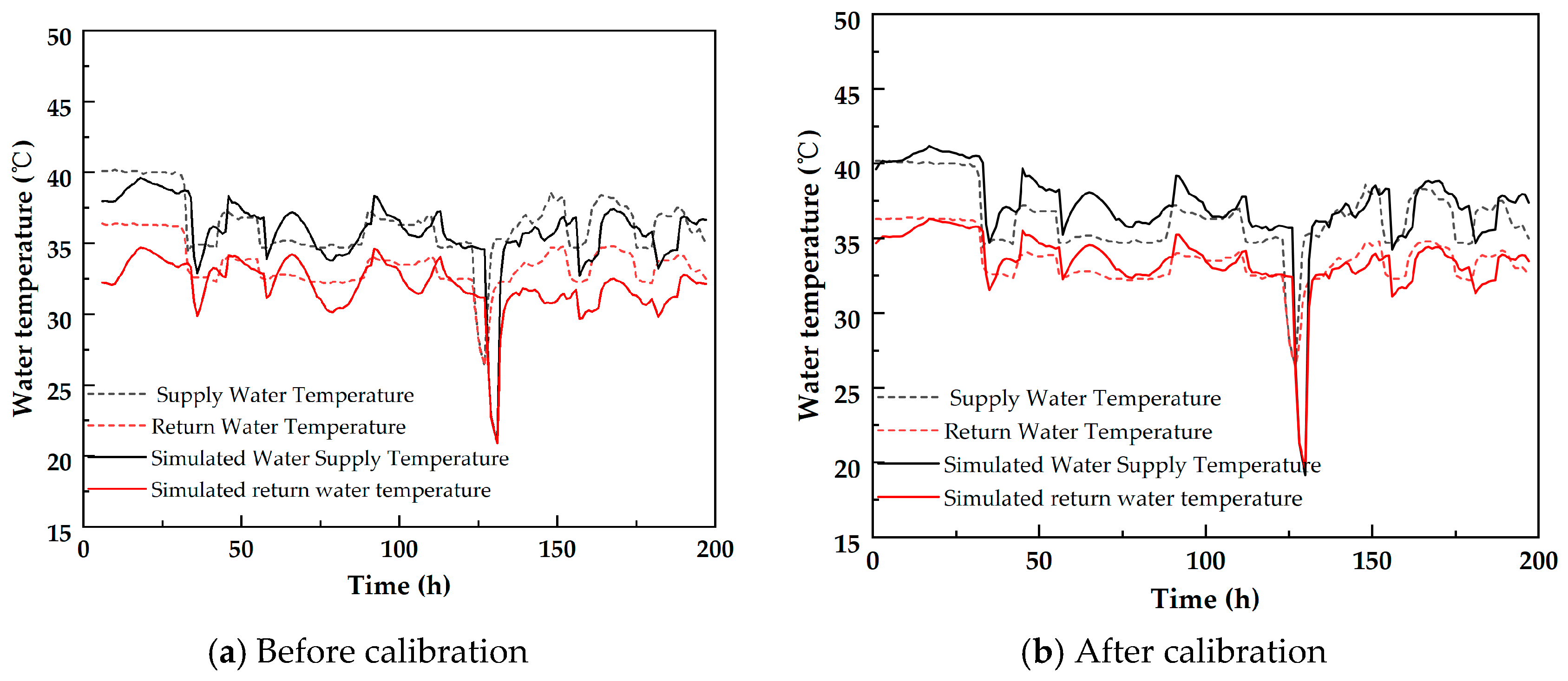
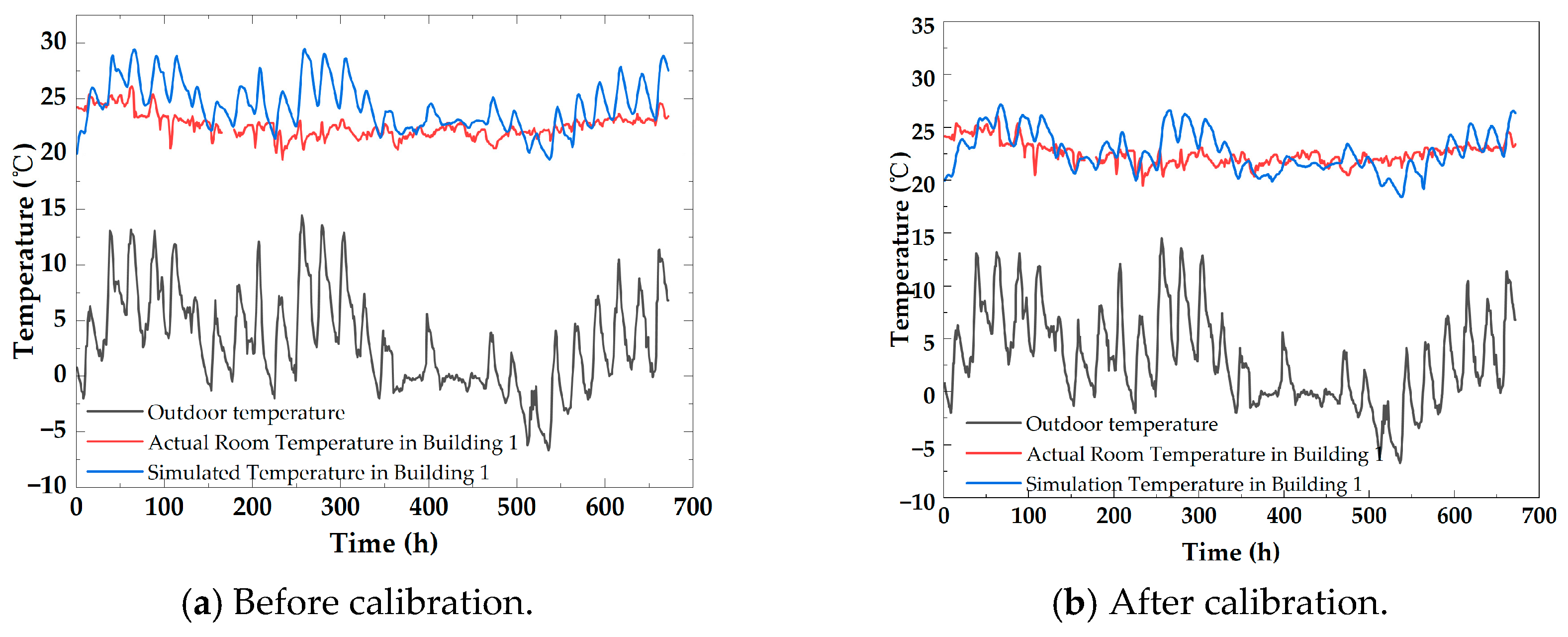
Model calibration was performed on the established secondary network architecture, with the primary network flow setpoints being systematically optimized. Figure 15 illustrates the comparative performance of the heating network model prior to and following calibration. Post-calibration, the simulated secondary supply and return temperatures exhibited a significantly improved fit with measured data, demonstrating that the model more accurately captures the thermal dynamics of the network and the resulting indoor temperatures.

The calculation results for the correlation evaluation indicators between simulated and actual measured return water temperatures of the secondary network supply in Building 1 before and after calibration are shown in

Table 4. Calculation table for each indicator before and after calibration.

Indicator	Pre-Calibration Value	Calibrated Value	Decline
MSE	5.02	2.54	49.40%
RMSE	2.43	1.59	34.60%
MAE	2.45	0.91	62.90%
RMD	6.61%	2.81%	57.50%

.

Post-calibration, all four core error evaluation metrics for the thermal network model exhibited significant improvement. Specifically, the MSE decreased by 49.4%, reflecting a substantially enhanced capability to minimize large deviations; meanwhile, the RMSE decreased by 34.6%, confirming a broad improvement in overall predictive accuracy. Notably, the MAE decreased by 62.9%, indicating that the error reduction is systemic rather than being driven solely by the correction of extreme data points. These improvements establish a more accurate and reliable foundation for the subsequent optimization and control of the heating network.

Table 5. Comparison of simulated and actual supply/return water temperature value calculation table.

Supply and Return Water Temperature Specifications (°C)	Building 1	Building 4	Building 5	Building 7
MSE	2.54	2.82	3.83	4.57
RMSE	1.59	1.68	1.96	2.14
MAE	0.91	1.28	1.63	1.83
RMD	2.81	3.95	5.05	5.07

presents a comparison between the simulated and measured secondary supply and return temperatures across several representative buildings.

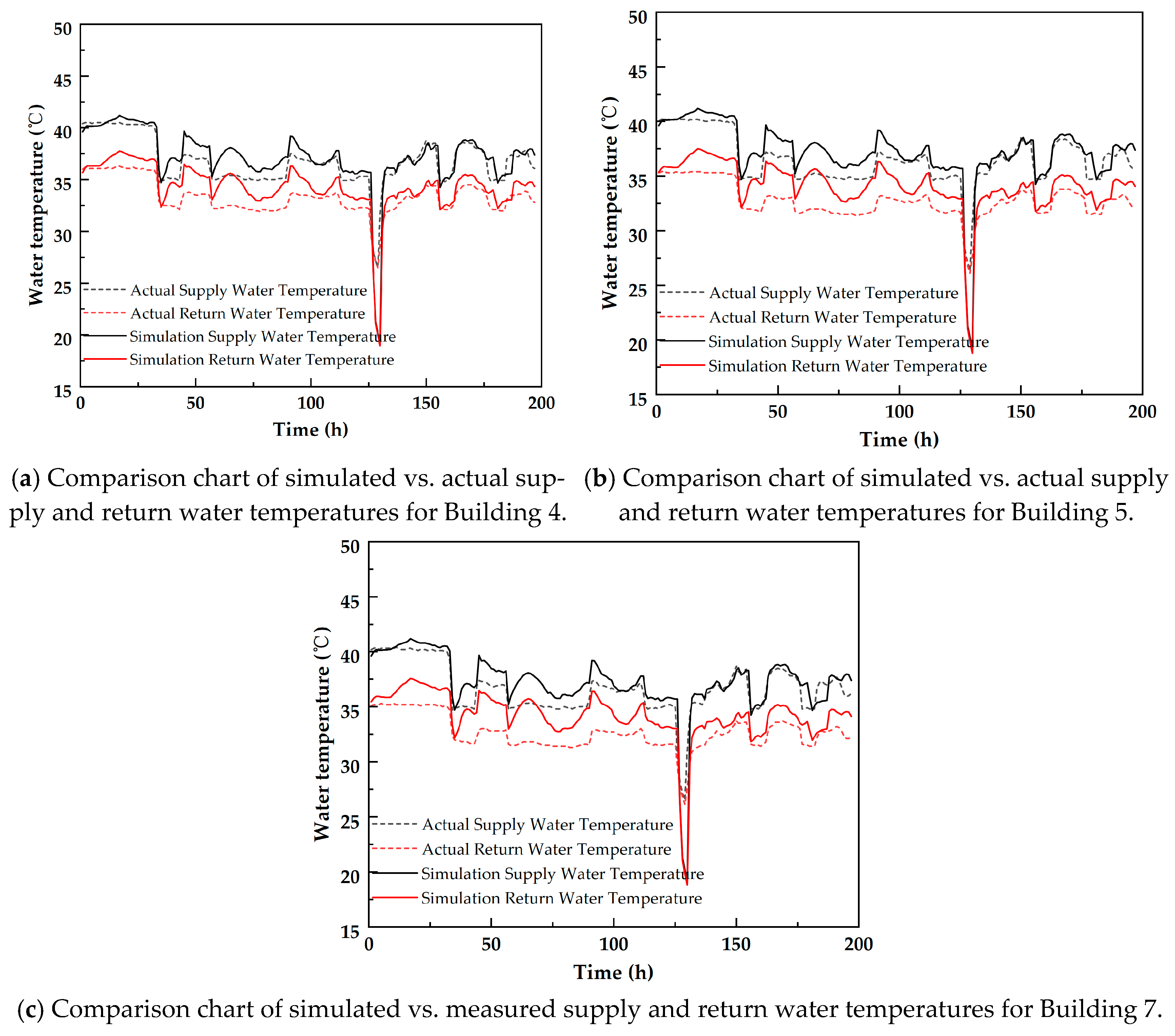
As the secondary network follows a radial distribution where each building (Buildings 1 through 8) represents an independent hydraulic branch, the validation was extended beyond Building 1. Specifically, the simulation results were compared against field measurements for the branches serving Buildings 4, 5, and 7. These comparative results are illustrated in Figure 16.

Building 1 is situated closest to the heat exchange station, with Buildings 4, 5, and 7 located at progressively greater distances. An analysis of the supply and return temperature simulation error metrics reveals a clear spatial correlation: buildings more proximal to the station demonstrate higher simulation accuracy, whereas those situated further away exhibit larger error margins. Crucially, it must be emphasized that the temperature deviations observed at these distal nodes do not indicate a deterioration in the model’s simulation accuracy; rather, they serve as a genuine reflection of the inherent physical and dynamic processes characterizing large-scale district heating networks. This distinct spatial trend carries profound physical and engineering implications, which are analyzed from multiple perspectives below.

During the thermal distribution process within the secondary network, heat transfer from the central station to individual buildings is subjected to several phenomenological factors: augmented thermal dissipation due to extended pipeline lengths, heterogeneous flow distribution, and dynamic response lags. As the transport distance increases, the persistent temperature gradient between the circulating hot water and the ambient environment induces a cumulative heat loss along the pipeline. This inherent heat dissipation causes the idealized simulated temperatures to typically overshoot the actual measured values, thereby inducing a deviation. Furthermore, within a multi-branch network topology, proximal buildings naturally secure a more stable flow allocation. In contrast, distal buildings are often subjected to substantial hydraulic resistance and pronounced pressure drops, causing the actual flow rates to fall below the design specifications, which further amplifies the discrepancy between the simulated and empirical data. Additionally, it is evident that under transient load conditions, the thermal response lag in the distant buildings is significantly more pronounced than in Building 1. Consequently, the distinct temperature response profiles exhibited by these distal buildings provide compelling evidence that the proposed high-fidelity physical model successfully captures the intricate spatial distribution dynamics of the heating network.

Due to the significant influence of building spatial location on the MPC control framework established in this study, the simulation accuracy decreases as the distance from the heat exchange station increases. Therefore, for district heating systems with dispersed building distributions, it is necessary and urgent to construct a more advanced architecture of distributed or layered MPC to improve simulation and regulation accuracy.

4.2.2. Dynamic Heat Load Prediction Model

Following the hydraulic calibration of the thermal network, the high-fidelity EnergyPlus model was coupled with the calibrated pipe network to simulate the indoor thermal response of Building 1. The resulting simulated indoor temperature profiles were compared against actual measurements, as illustrated in Figure 17.

As illustrated in Figure 17, the accuracy of the simulated indoor temperatures improves significantly following the calibration of the heating network model. Furthermore, relevant evaluation metrics comparing the simulated and actual measured indoor temperatures for Building 1, both before and after calibration, were calculated. These results are summarized in

Table 6. Comparison of the indoor temperature evaluation metrics for Building 1 pre- and post-calibration.

Indicator	Pre-Calibration Value	Calibrated Value	Decline
MSE	4.41 °C	3.13 °C	↓ 29.0%
RMSE	2.10 °C	1.77 °C	↓ 15.0%
MAE	1.62 °C	1.38 °C	↓ 14.8%
RMD	6.97%	6.18%	↓ 11.3%

.

According to Table 6, the MSE decreased from 4.41 to 3.13 (a 29.0% reduction), reflecting an enhanced capability to mitigate large deviations. The RMSE decreased from 2.10 to 1.77 (a 15.7% reduction), confirming the overall improvement in predictive accuracy. A 14.8% reduction in MAE, which is consistent with the RMSE improvement, suggests that the error reduction is uniform across the dataset rather than being driven by a few isolated outliers.

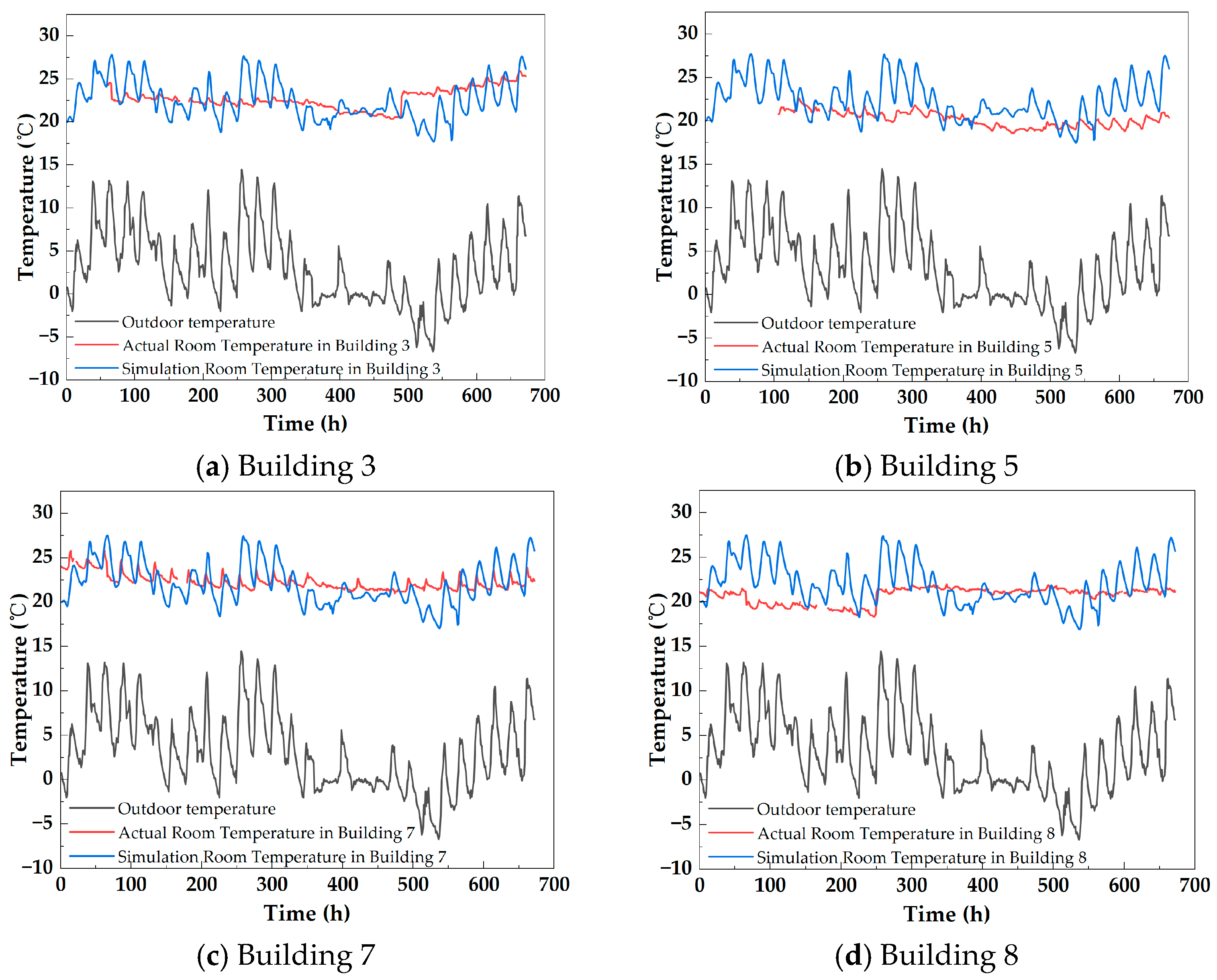
As illustrated in Figure 16, the skewness of the error distribution shifted from 1.2 to 0.8, demonstrating that systematic overestimation—where simulated temperatures consistently exceeded measured values—was successfully mitigated. The kurtosis similarly decreased from 4.1 to 3.3, reflecting a more concentrated error distribution with fewer extreme residuals. These findings align with the significant reduction in MSE, proving that calibration corrected both the systematic bias and the overall dispersion of the error. Furthermore, the indoor thermal response of several additional buildings was simulated and validated against field measurements, as shown in Figure 18.

Based on the simulated and measured indoor temperatures for each building, corresponding error evaluation metrics were calculated and are listed in

Table 7. Comparison of simulated and actual room temperatures for heating users.

Parameters	Building 1	Building 3	Building 5	Building 7	Building 8
MSE	3.13 °C	3.42 °C	7.57 °C	5.18 °C	5.51 °C
RMSE	1.77 °C	1.85 °C	2.75 °C	2.27 °C	2.35 °C
MAE	1.38 °C	1.51 °C	2.28 °C	1.85 °C	1.86 °C
RMD	6.18 °C	6.62 °C	11.35 °C	8.37 °C	9.08 °C

.

An analysis of the error metrics presented in Table 6 reveals distinct spatial variations in the simulated indoor thermal profiles across the five buildings. Notably, Building 1 exhibits the highest simulation fidelity, achieving a Mean Squared Error (MSE) of 3.13 and a Mean Absolute Error (MAE) of 1.38 °C. Conversely, Building 5 demonstrates the maximum simulation discrepancy, with its MSE and MAE escalating to 7.57 and 2.28 °C, respectively.

Nevertheless, by rigorously integrating the complex effects of building thermal inertia, spatial temperature gradients, and stochastic occupant behaviors, the calibrated district heating network model yields simulation results that align robustly with the empirical measurements. Consequently, the proposed model proves highly capable of capturing the transient dynamics of the indoor thermal field, thereby validating its robust applicability for advanced simulation-based analysis and the optimal regulation of building thermal environments.

4.3. Evaluation of MPC Methods in Actual Engineering Projects

4.3.1. Evaluation of MPC Experimental Results

As shown in

Table 8. Comparison of different operating conditions.

Operating Conditions	Comfort Index	Temperature Control Accuracy (°C)	System Stability (°C)
Operating Condition A	100%	0.29	0.30
Operating Condition B	100%	0.49	0.38

, a comparative analysis of the performance metrics under the two operating conditions reveals that in Case Study A, the supply water flow rate is utilized as the direct control variable, resulting in a relatively straightforward control logic. The system tracks the indoor temperature setpoint by modulating the secondary-side mass flow rate. The simulation results indicate two primary advantages of this approach:

Rapid dynamic response: Direct regulation of the mass flow rate enables near-instantaneous compensation for load demands or temperature fluctuations, thereby minimizing the settling time required to maintain indoor thermal comfort.

High setpoint tracking precision: Direct flow adjustment to satisfy thermal requirements yields superior control precision, as evidenced by a minimal temperature deviation of only 0.29 °C in Scenario A.

However, quantity regulation (flow-based control) has inherent limitations; it neglects the impact of building thermal mass and distribution network thermal lag, which may lead to transient overshoot or hydraulic instability during abrupt demand fluctuations.

In Case Study B, the secondary network supply temperature is modulated by adjusting the primary network mass flow rate, resulting in the indirect regulation of indoor temperature. Experimental results indicate that modulating primary flow to control secondary supply temperatures mitigates hydraulic fluctuations, particularly during partial-load periods. This mechanism effectively reduces parasitic energy losses and enhances the aggregate energy efficiency of the system.

However, this indirect control strategy exhibits specific limitations. Due to a more constrained comfort range, the thermal comfort index for Case Study B is lower than that of Case Study A, suggesting a sluggish thermal response relative to direct flow regulation. Due to the inherent thermal lag within the distribution network, adjustments to the primary circuit require significant lead time to affect secondary temperatures, which may induce transient thermal oscillations during abrupt load shifts. Additionally, the temperature control precision is reduced; as an indirect method, the heat transfer chain involves multiple coupled stages and is subject to cumulative uncertainties. These factors can lead to temporary setpoint deviations during periods of high demand volatility. In conclusion, while indirect quality regulation improves hydraulic stability, direct quantity control at the terminal level provides superior setpoint tracking precision and enhanced system stability.

4.3.2. Comparison of Regulation Capabilities Under Different Operating Conditions

To rigorously evaluate the performance benefits and practical engineering value of the proposed model predictive control (MPC) strategy, this study establishes the system’s actual historical operating conditions prior to MPC implementation as the baseline scenario (designated as “Without MPC”). Specifically, this baseline system operates on a conventional manual adjustment strategy guided by a weather compensation curve. In actual district heating practice, station operators manually modulate the supply temperature setpoint of the primary network and the total flow rate of the secondary network in response to outdoor dry-bulb temperature fluctuations, relying on an empirical climate compensation curve. Fundamentally, this traditional control paradigm is passively reactive. It is devoid of predictive capabilities regarding impending meteorological shifts, internal heat gains, and the substantial thermal inertia inherent in both the building envelopes and the distribution network. Consequently, it is highly susceptible to pronounced control lag when subjected to dynamic thermal loads.

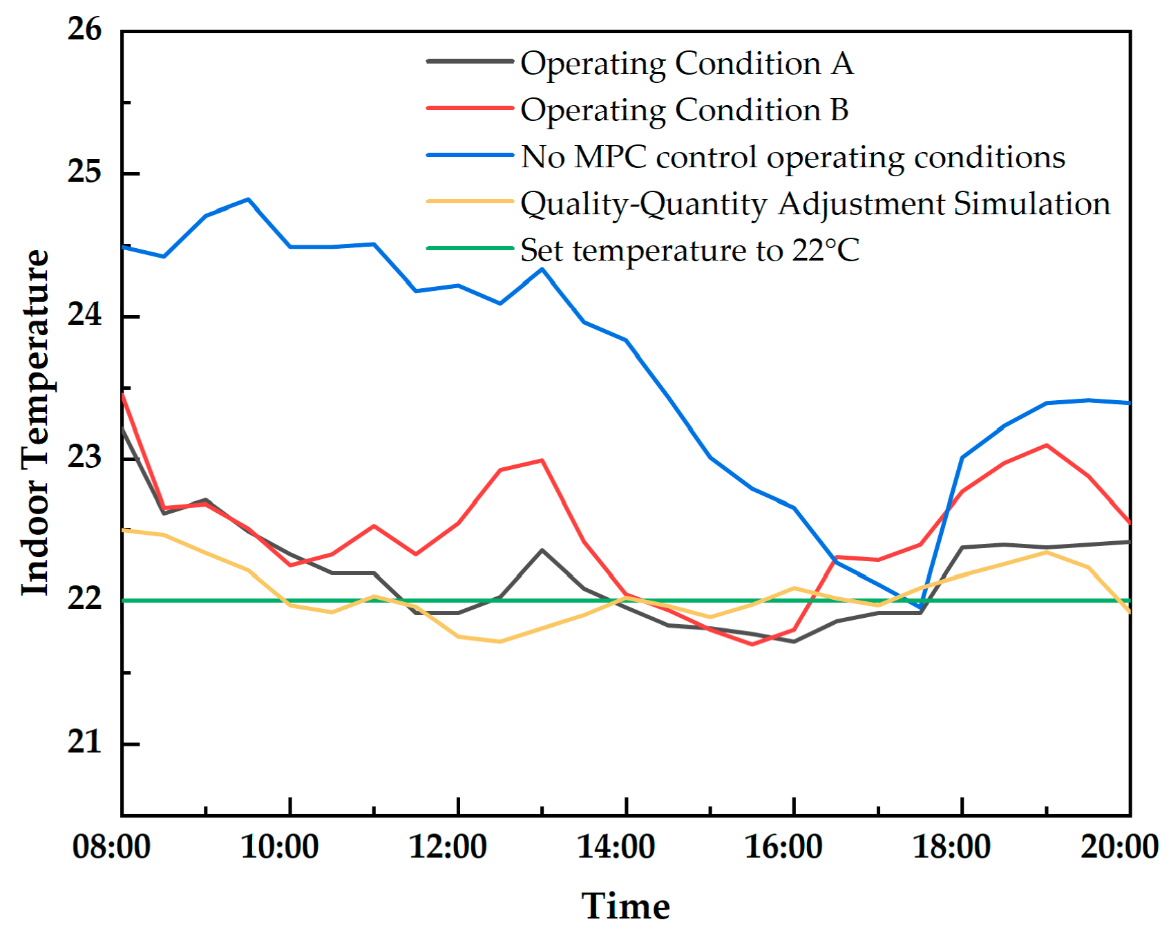
Based on the system’s actual measurement data comparison, under similar outdoor weather conditions (with measurements taken on close dates), indoor temperature data was collected from Room 1602, Unit 2, Building 1 from 8:00 AM to 8:00 PM. The results are shown in the figure below:

As illustrated in Figure 19, the baseline scenario (without MPC regulation) exhibited prolonged periods of excessive indoor temperatures. During the afternoon, a decrease in ambient temperature triggered a significant drop in indoor temperatures, with fluctuations of approximately 2–3 °C. Such volatility can adversely impact thermal comfort levels for the occupants. After 18:00, a consistent temperature rebound is observed across all profiles; this is attributed to increased internal heat gains from occupant activity as residents return home, resulting in a rising thermal trend.

To conduct a rigorous comparative analysis based on empirical data, diurnal indoor temperature profiles were recorded for Unit 2-1602 in Building 1. These measurements were conducted from 8:00 AM to 8:00 PM under quasi-steady ambient weather conditions on consecutive dates to ensure environmental boundary consistency. The resulting temporal temperature fluctuations are illustrated in the figure below.

Under both Case Studies A and B, the indoor temperature consistently remained within the specified comfort range. This indicates that the calibrated MPC framework effectively stabilizes indoor temperatures, ensuring high levels of thermal comfort for the occupants. Notably, the MPC strategy significantly enhances thermal comfort by mitigating transient temperature fluctuations. Furthermore, both operating conditions exhibit superior system stability, characterized by low standard deviations, reflecting minimal setpoint residuals during steady-state operation, as shown in

Table 9. Comparative analysis of tables with and without MPC adjustment.

Operating Conditions	Comfort Time Percentage	System Stability (°C)
Actual operating condition A	100%	0.30
Actual operating condition B	100%	0.38
MPC mass regulation simulation operating conditions	100%	0.15
Actual operating conditions without MPC regulation	56%	0.86

.

In the absence of MPC control, the comfort index drops precipitously to 56%, demonstrating that the conventional system fails to maintain a stable thermal environment. This results in chronic overheating, significant parasitic energy waste, and pronounced indoor temperature fluctuations. Furthermore, comparative simulations under identical boundary conditions revealed that the integrated quality–quantity (mass–temperature) MPC mode demonstrated robust performance. The system maintained steady-state operation within the comfort range, exhibiting superior thermal regulation compared to traditional control methods.

The implementation of the MPC strategy markedly enhances overall heating system performance, consistently delivering superior thermal comfort, high-precision setpoint tracking, and enhanced system stability across a range of operating conditions. In contrast, the conventional system (lacking MPC) exhibits significant operational deficiencies, specifically regarding temperature control precision and hydraulic stability. These limitations result in substantial thermal fluctuations and a marked degradation in occupant comfort.

5. Conclusions

This study presents an MPC framework based on a source-network-load co-simulation model, validated using a residential heating system in Xinzheng City, Henan Province, China, as a representative engineering case. The MPC architecture integrates Dymola with GenOpt, while coupling EnergyPlus and Modelica to achieve holistic control of the heating system. By implementing a zoned thermal balance modeling approach, the numerical instability and predictive inaccuracies inherent in traditional methods are effectively mitigated. The conclusions are summarized as follows:

(1) Integrated co-simulation significantly enhances predictive accuracy. This platform enables the concurrent computation of hydraulic–thermal dynamics within the network and the building’s thermal response, establishing a high-fidelity simulation environment for robust MPC strategy development. Furthermore, inverse parameter identification using GenOpt significantly increases the reliability and practical applicability of the model.

(2) Data-driven calibration of the co-simulation framework significantly enhances model performance. Post-calibration, the secondary network supply and return temperature residuals for Building 1 showed substantial reductions: the MSE, RMSE, and MAE decreased by 49.4%, 34.6%, and 62.9%, respectively. Simultaneously, the predictive accuracy for indoor temperature was significantly refined, with the RMSE improving by 15.7%, RMD decreasing from 6.97% to 6.18%, and MSE and MAE dropping by 29.0% and 14.8%.

(3) The validated model reveals distinct spatial characteristics with significant engineering implications. Simulation accuracy is positively correlated with proximity to the heat exchange station, with Building 1 showing an MSE of 2.54, while distal nodes such as Building 7 reached 4.57. Concurrently, thermal propagation delays result in increased deviations in distal buildings; for example, Building 5 exhibited an indoor temperature MAE of 2.28 °C, representing a 65% increase over Building 1. These results validate the effectiveness of the proposed system bias correction in capturing the complex dynamics of a multi-branch network.

(4) The proposed source-network-load integrated MPC framework significantly enhances thermal comfort and hydraulic stability. In practical application, the direct quantity regulation strategy (Case Study A) demonstrates significant advantages over indirect quality regulation (Case Study B), achieving a 41.5% enhancement in temperature tracking precision and a 22.2% improvement in operational stability. Relative to the baseline system, the MPC strategy optimized the comfort index from 56% to 100% and reduced temperature fluctuations from 0.86 °C to 0.15 °C, effectively suppressing temperature overshoot and oscillations. This methodology establishes a standardized framework for the optimization of large-scale district heating systems.

It is worth noting that the current MPC framework relies on the iterative execution of the comprehensive, high-fidelity Dymola–EnergyPlus co-simulation model, which imposes a substantial computational burden (e.g., evaluating a 24 h prediction horizon requires several hours of computation time). Consequently, the proposed strategy currently functions as an offline optimization framework, designed to compute the optimal day-ahead control sequence in advance. To transition this framework toward real-time online control, our future work will focus on developing a computationally efficient, data-driven surrogate model trained on datasets generated by the present high-fidelity white-box model. Such an integration is anticipated to drastically curtail optimization runtime, thereby paving the way for the practical implementation of real-time dynamic control.

References

1. Castro, V.; Georgiou, M.; Jackson, T.; Hodgkinson, I.R.; Jackson, L.; Lockwood, S. Digital Data Demand and Renewable Energy Limits: Forecasting the Impacts on Global Electricity Supply and Sustainability. Energy Policy 2024, 195, 114404. [Google Scholar] [CrossRef]
2. Khurshid, A.; Khan, K.; Rauf, A.; Cifuentes-Faura, J. Energy Transitions, Carbon Emissions, and Network Effects: A Multiphase Analysis of Global Industrial Resilience. J. Environ. Manag. 2025, 393, 126945. [Google Scholar] [CrossRef]
3. Chen, L.; Zhao, Y.; Xie, R.; Su, B.; Liu, Y.; Renfei, X. Embodied Energy Intensity of Global High Energy Consumption Industries: A Case Study of the Construction Industry. Energy 2023, 277, 127628. [Google Scholar] [CrossRef]
4. Chen, C.; Cao, X.; Zhang, S.; Lei, Z.; Zhao, K. Dynamic Characteristic and Decoupling Relationship of Energy Consumption on China’s Construction Industry. Buildings 2022, 12, 1745. [Google Scholar] [CrossRef]
5. Idrissi Kaitouni, S.; Romani, Z.; Jamil, A.; Ahachad, M. Zero Carbon Urban Buildings (ZCUBs) in the Era of Climate Change, Digital Transformation and Energy Transition: A Scoping Review from 2000 to 2024. Build. Environ. 2025, 280, 113116. [Google Scholar] [CrossRef]
6. Siu, C.Y.; Brown, S.; Brideau, S.; Ji, L.; O’Brien, W.; Ferguson, A.; Greco, E.; Touchie, M.; Mclellan, C.; Lepage, R.; et al. Exploring the Role of Building Codes in Protecting Occupants from Overheating—A Canadian Perspective. Energy Build. 2025, 338, 115673. [Google Scholar] [CrossRef]
7. Tahir, F.; Sexton, C.E.; Al-Ghamdi, S.G. 1.07-Energy, Climate Change and Built Environment. In Comprehensive Energy Systems; Dincer, I., Ed.; Elsevier: Oxford, UK, 2025; pp. 136–166. ISBN 978-0-443-34108-3. [Google Scholar]
8. Hachez, J.; Latiers, A.; Berger, B.; Bram, S. Multi-Energy Systems Fast Optimization: A New Formulation in Linear Programming for Temperatures and Magnitudes of Thermal Power Flows in Heating Systems. Energy Build. 2025, 336, 115618. [Google Scholar] [CrossRef]
9. Cid, J.M.; Mylonas, A.; Péan, T.Q.; Pascual, J.; Salom, J. Energy Optimization Algorithms for Multi-Residential Buildings: A Model Predictive Control Application. Energy Build. 2024, 319, 114562. [Google Scholar] [CrossRef]
10. Zhu, Y.; Zhang, Q.; Zeng, L.; Wang, J.; Zou, S.; Zheng, H. An Advanced Control Strategy for Optimizing the Operation State of Chillers with Cold Storage Technology in Data Center. Energy Build. 2023, 301, 113684. [Google Scholar] [CrossRef]
11. Wang, Z.; Chen, H.; Sun, X.; Lu, H.; Wang, T. Optimizing the Solar-Air Hybrid Source Heat Pump Heating System Based on the Particle Swarm Algorithm. Energy Rep. 2022, 8, 379–393. [Google Scholar] [CrossRef]
12. Nasouri, M.; Delgarm, N. Numerical Modeming, Energy–Exergy Analyses, and Multi-Objective Programming of the Solar-Assisted Heat Pump System Using Genetic Algorithm Coupled with the Multi-Criteria Decision Analysis. Arab. J. Sci. Eng. 2023, 48, 3537–3557. [Google Scholar] [CrossRef]
13. Soleimani, A.; Davidsson, P.; Malekian, R.; Spalazzese, R. Modeling Hybrid Energy Systems Integrating Heat Pumps and District Heating: A Systematic Review. Energy Build. 2025, 329, 115253. [Google Scholar] [CrossRef]
14. Kiss, G.R.; Horváth, M.; Szánthó, Z. MATLAB Simulink-Based Modelling and Performance Analysis of District Heating Substations for Renewable Energy Integration. Energies 2025, 18, 2370. [Google Scholar] [CrossRef]
15. Petrov, A.; Popov, A. Visualization of Physical and Mathematical Models of Thermodynamic Processes of Single-Phase Flows Using MATLAB to Diagnose the Condition of External Heat Supply Networks. J. Phys. Conf. Ser. 2021, 2131, 052069. [Google Scholar] [CrossRef]
16. Sun, Z.; Liu, D.; Yuan, H.; Sun, Z.; Pan, W.; Zhang, Z.; Ma, B.; Jiang, Z. The Water Hammer in the Long-Distance Steam Supply Pipeline: A Computational Fluid Dynamics Simulation. Cogent Eng. 2022, 9, 2127472. [Google Scholar] [CrossRef]
17. Lee, J.-S.; Rhi, S.-H.; Kim, S.-K. Modeling and Simulation of Heat Pipes: Review. J. Mech. Sci. Technol. 2024, 38, 2591–2612. [Google Scholar] [CrossRef]
18. Anbarasu, S.; Hinkelman, K.; Zuo, W. Thermo-Hydraulic Steam Pipe Models for District Heating Simulations: Simplifications to Balance Accuracy and Simulation Speed. Build. Simul. 2025, 18, 2151–2174. [Google Scholar] [CrossRef]
19. Li, C.; Prasad, S.; Bai, Y.; Turkeri, C.; Wang, J. A Quasi-Dynamic Model and Comprehensive Simulation Study of District Heating Networks Considering Temperature Delay. Energy 2025, 318, 134855. [Google Scholar] [CrossRef]
20. Calixto, S.; Köseoğlu, C.; Cozzini, M.; Manzolini, G. Monitoring and Aggregate Modelling of an Existing Neutral Temperature District Heating Network. Energy Rep. 2021, 7, 140–149. [Google Scholar] [CrossRef]
21. Xu, Q.; Wang, K.; Zou, Z.; Zhong, L.; Akkurt, N.; Feng, J.; Xiong, Y.; Han, J.; Wang, J.; Du, Y. A New Type of Two-Supply, One-Return, Triple Pipe-Structured Heat Loss Model Based on a Low Temperature District Heating System. Energy 2021, 218, 119569. [Google Scholar] [CrossRef]
22. Vieth, J.; Westphal, J.; Speerforck, A. District Heating Network Topology Optimization and Optimal Co-Planning Using Dynamic Simulations. Adv. Appl. Energy 2025, 19, 100233. [Google Scholar] [CrossRef]
23. Meibodi, S.S.; Rees, S.; Loveridge, F. Modeling District Heating Pipelines Using a Hybrid Dynamic Thermal Network Approach. Energy 2024, 290, 130107. [Google Scholar] [CrossRef]
24. Yang, W.; Shi, J.; Li, S.; Song, Z.; Zhang, Z.; Chen, Z. A Combined Deep Learning Load Forecasting Model of Single Household Resident User Considering Multi-Time Scale Electricity Consumption Behavior. Appl. Energy 2022, 307, 118197. [Google Scholar] [CrossRef]
25. Moradzadeh, A.; Mohammadi-Ivatloo, B.; Abapour, M.; Anvari-Moghaddam, A.; Roy, S.S. Heating and Cooling Loads Forecasting for Residential Buildings Based on Hybrid Machine Learning Applications: A Comprehensive Review and Comparative Analysis. IEEE Access 2022, 10, 2196–2215. [Google Scholar] [CrossRef]
26. Yan, R.; Wang, J.; Lu, S.; Ma, Z.; Zhou, Y.; Zhang, L.; Cheng, Y. Multi-Objective Two-Stage Adaptive Robust Planning Method for an Integrated Energy System Considering Load Uncertainty. Energy Build. 2021, 235, 110741. [Google Scholar] [CrossRef]
27. Potočnik, P.; Škerl, P.; Govekar, E. Machine-Learning-Based Multi-Step Heat Demand Forecasting in a District Heating System. Energy Build. 2021, 233, 110673. [Google Scholar] [CrossRef]
28. Ghilardi, L.M.P.; Castelli, A.F.; Moretti, L.; Morini, M.; Martelli, E. Co-Optimization of Multi-Energy System Operation, District Heating/Cooling Network and Thermal Comfort Management for Buildings. Appl. Energy 2021, 302, 117480. [Google Scholar] [CrossRef]
29. Huo, S.; Wang, J.; Qin, Y.; Cui, Z. Operation Optimization of District Heating Network under Typical Modes for Improving the Economic and Flexibility Performances of Integrated Energy System. Energy Convers. Manag. 2022, 267, 115904. [Google Scholar] [CrossRef]
30. Abraham, A.; Madureira, A.M.; Kaklauskas, A.; Gandhi, N.; Bajaj, A.; Muda, A.K.; Kriksciuniene, D.; Ferreira, J.C. (Eds.) Innovations in Bio-Inspired Computing and Applications: Proceedings of the 12th International Conference on Innovations in Bio-Inspired Computing and Applications (IBICA 2021) Held during December 16–18, 2021; Lecture Notes in Networks and Systems; Springer International Publishing: Cham, Switzerland, 2022; Volume 419, ISBN 978-3-030-96298-2. [Google Scholar]
31. Su, G.; Peng, Y.; Yao, W.; Zhang, S. Distributed Control Strategy of Central Heating System Based on Multi-Agent Consensus. Appl. Therm. Eng. 2025, 262, 125136. [Google Scholar] [CrossRef]
32. Freund, S.; Schmitz, G. Implementation of Model Predictive Control in a Large-Sized, Low-Energy Office Building. Build. Environ. 2021, 197, 107830. [Google Scholar] [CrossRef]
33. Cao, Z.; Han, X.; Lyons, W.; O’Rourke, F. Energy Management Optimisation Using a Combined Long Short-Term Memory Recurrent Neural Network–Particle Swarm Optimisation Model. J. Clean. Prod. 2021, 326, 129246. [Google Scholar] [CrossRef]
34. Wu, M.; Du, P.; Jiang, M.; Goh, H.H.; Zhu, H.; Zhang, D.; Wu, T. An Integrated Energy System Optimization Strategy Based on Particle Swarm Optimization Algorithm. Energy Rep. 2022, 8, 679–691. [Google Scholar] [CrossRef]
35. Wang, Y.; Li, Z.; Liu, J.; Zhao, Y.; Sun, S. A Novel Combined Model for Heat Load Prediction in District Heating Systems. Appl. Therm. Eng. 2023, 227, 120372. [Google Scholar] [CrossRef]
36. Khan, O.; Parvez, M.; Seraj, M.; Yahya, Z.; Devarajan, Y.; Nagappan, B. Optimising Building Heat Load Prediction Using Advanced Control Strategies and Artificial Intelligence for HVAC System. Therm. Sci. Eng. Prog. 2024, 49, 102484. [Google Scholar] [CrossRef]
37. Wang, Y.; Zhan, C.; Li, G.; Ren, S. Comparison of Algorithms for Heat Load Prediction of Buildings. Energy 2024, 297, 131318. [Google Scholar] [CrossRef]
38. Sun, J.; Gong, M.; Zhao, Y.; Han, C.; Jing, L.; Yang, P. A Hybrid Deep Reinforcement Learning Ensemble Optimization Model for Heat Load Energy-Saving Prediction. J. Build. Eng. 2022, 58, 105031. [Google Scholar] [CrossRef]
39. Song, J.; Zhang, L.; Xue, G.; Ma, Y.; Gao, S.; Jiang, Q. Predicting Hourly Heating Load in a District Heating System Based on a Hybrid CNN-LSTM Model. Energy Build. 2021, 243, 110998. [Google Scholar] [CrossRef]
40. Cui, X.; Zhu, J.; Jia, L.; Wang, J.; Wu, Y. A Novel Heat Load Prediction Model of District Heating System Based on Hybrid Whale Optimization Algorithm (WOA) and CNN-LSTM with Attention Mechanism. Energy 2024, 312, 133536. [Google Scholar] [CrossRef]
41. Dong, L.; Wei, J.; Lin, H.; Wang, X. Distributed Optimization of Electricity-Gas-Heat Integrated Energy System with Multi-Agent Deep Reinforcement Learning. Glob. Energy Interconnect. 2022, 5, 604–617. [Google Scholar] [CrossRef]
42. Meng, H.; Liu, J.; Shang, W.; Xu, J.; Jia, L. Multi-Agent Distributed Control Method for Clean Air-Conditioning Systems: Balancing Cleanliness, Pressure and Energy Consumption. J. Build. Eng. 2025, 107, 112806. [Google Scholar] [CrossRef]
43. Weng, K.; Ren, Y.; Zhao, L.; Gao, S. Distributed Optimization of Multi-Agent Systems with Time-Invariant and Time-Varying Cost Functions. Eur. J. Control 2025, 83, 101222. [Google Scholar] [CrossRef]
44. Wetter, M.; Zuo, W.; Nouidui, T.S.; Pang, X. Modelica Buildings Library. J. Build. Perform. Simul. 2014, 7, 253–270. [Google Scholar] [CrossRef]
45. Walker, S.; Katic, K.; Maassen, W.; Zeiler, W. Multi-Criteria Feasibility Assessment of Cost-Optimized Alternatives to Comply with Heating Demand of Existing Office Buildings–A Case Study. Energy 2019, 187, 115968. [Google Scholar] [CrossRef]
46. Zhang, L.; Gudmundsson, O.; Thorsen, J.E.; Li, H.; Li, X.; Svendsen, S. Method for Reducing Excess Heat Supply Experienced in Typical Chinese District Heating Systems by Achieving Hydraulic Balance and Improving Indoor Air Temperature Control at the Building Level. Energy 2016, 107, 431–442. [Google Scholar] [CrossRef]
47. Tian, X.; Lin, X.; Zhong, W.; Zhou, Y.; Cong, F. Optimal Dispatch of Integrated Electricity and Heating Systems Considering the Quality-Quantity Regulation of Heating Systems to Promote Renewable Energy Consumption. Energy 2024, 300, 131599. [Google Scholar] [CrossRef]
Figure 1. First-order equivalent RC model of the building.
Energies 19 02096 g001
Figure 2. Modelica and EnergyPlus joint module.
Energies 19 02096 g002
Figure 3. Hydraulic–thermal coupling simulation model.
Energies 19 02096 g003aEnergies 19 02096 g003b
Figure 4. Physical model of Building 4 in the study subject.
Energies 19 02096 g004
Figure 5. Secondary network joint simulation model considering outage rates.
Energies 19 02096 g005
Figure 6. Schematic diagram of GenOpt optimization.
Energies 19 02096 g006
Figure 7. White-box MPC construction flowchart.
Energies 19 02096 g007
Figure 8. Flowchart of the proposed MPC strategy.
Energies 19 02096 g008
Figure 9. Construction of the quality adjustment objective function.
Energies 19 02096 g009
Figure 10. Optimization convergence plot of the GenOpt quality adjustment objective function.
Energies 19 02096 g010
Figure 11. Construction of quality-mass regulation objective function.
Energies 19 02096 g011
Figure 12. Convergence plot of GenOpt quality–quantity adjustment objective function optimization.
Energies 19 02096 g012
Figure 13. Simplified schematic diagram of the heating process.
Energies 19 02096 g013
Figure 14. Model calibration process for joint simulation optimization.
Energies 19 02096 g014
Figure 15. Comparison of simulated and measured supply and return water temperatures in Building 1 before and after calibration.
Energies 19 02096 g015
Figure 16. Comparison of simulated and measured supply and return water temperatures for secondary heating networks in representative buildings.
Energies 19 02096 g016
Figure 17. Comparison of simulated and actual room temperatures in Building 1 heat users’ rooms before and after calibration.
Energies 19 02096 g017
Figure 18. Comparison of simulated vs. actual room temperatures in representative building units.
Energies 19 02096 g018
Figure 19. Comparison of measured and simulated indoor temperature with and without MPC optimization.
Energies 19 02096 g019