Benchmarking 0D, 1D, and 2D Analytical Thermal Models for Cylindrical Inductors in Power Electronic Systems

Abstract

Inductors are critical components in power electronic systems, yet their thermal behavior is often approximated using simplified lumped models that neglect internal gradients and transient spatial effects. This paper presents a benchmarking study of analytical thermal modeling approaches for cylindrical inductors, including 0D lumped, 1D radial, and 2D radial–axial transient formulations. Starting from the general heat conduction equation in cylindrical coordinates, closed-form or semi-analytical solutions are discussed under uniform internal heat generation and convective boundary conditions. The proposed framework provides a benchmark-oriented analytical reference for selecting the appropriate thermal model complexity in reliability-oriented design of inductive components in power electronic systems. The models are applied to a representative two-layer cylindrical inductor composed of a ferrite core and a copper winding, under identical loss and cooling assumptions, considering two axial lengths in order to assess geometric influence. Steady-state temperature levels, transient responses, modal time constants, and axial gradient indicators are extracted to quantify the differences among modeling levels. The results show that the dominant thermal behavior is governed by a single slow mode with a time constant on the order of one hour. The spatially averaged temperature predicted by the 0D model deviates by less than 2.5% from the 2D solution in steady-state conditions, with the 1D model providing accurate predictions when axial gradients remain weak.

1. Introduction

Power electronic converters and systems are a basis of modern energy conversion and management, enabling high efficiency, controllability, and compactness in a wide range of applications, including renewable energy systems, electric transportation, industrial automation, and data centers [1,2,3,4]. The persistent demand for higher power density and increased switching frequency has led to a substantial rise in thermal stress, making thermal management a primary design constraint rather than a secondary verification step.

The overall performance and lifetime of power electronic converters are determined by the combined behavior of semiconductor devices, inductive components, and capacitors. Over the last decades, electro–thermal modeling of power semiconductors has been extensively investigated, leading to mature modeling techniques ranging from lumped thermal networks to detailed multi-dimensional finite-element (FE) models [5,6,7]. Similarly, capacitors, particularly electrolytic and film technologies, have been widely studied due to their strong temperature-dependent aging mechanisms, resulting in consolidated thermal and lifetime models that are routinely employed in reliability-oriented design [8,9,10].

Thermal design is tightly linked to both operational limits and long-term reliability. Excessive temperature rise and thermal cycling accelerate well-known degradation mechanisms, such as bond-wire fatigue and solder joint failure in power devices, dielectric breakdown and electrolyte evaporation in capacitors, and insulation aging and core degradation in magnetic components [11,12]. Consequently, accurate thermal modeling is essential not only to ensure safe operating conditions but also to support lifetime prediction and reliability-aware converter design.

Despite their essential role, inductive components remain comparatively under-represented in the thermal modeling literature, especially when contrasted with semiconductors and capacitors. Inductors and transformers are often the largest and heaviest components in power converters and are frequently responsible for a significant portion of total losses. Unlike semiconductor devices, however, inductive components exhibit distributed loss mechanisms, originating from both windings (DC and AC copper losses) and magnetic cores (hysteresis and eddy-current losses), which are spatially non-uniform and strongly dependent on operating conditions [13,14]. This intrinsic distribution makes simplified thermal representations particularly challenging.

Several studies have addressed the thermal behavior of capacitors and magnetic components using lumped or reduced-order thermal models, often based on equivalent thermal resistance–capacitance (RC) networks identified from experimental measurements or steady-state assumptions [15,16,17,18]. In particular, cylindrical and axisymmetric geometries, typical of wound inductors, toroidal cores, and certain capacitor constructions, have been investigated through analytical or semi-analytical approaches focusing on radial heat conduction and average temperature rise [19,20]. These methods provide valuable insight but are typically limited to steady-state conditions or global temperature estimation.

Efficient thermal management of inductive components is particularly critical in high-frequency power converters employed in electric mobility and renewable energy systems, where compactness and elevated power density exacerbate thermal stress. While one-dimensional or semi-analytical thermal models have been shown to provide accurate steady-state temperature predictions for cylindrical magnetic components [21,22], they inherently fail to capture axial heat conduction and dynamic temperature gradients arising under transient loading conditions.

Recent studies on multi-dimensional electro–thermal analysis of power semiconductor devices and magnetic components have demonstrated that lateral heat spreading and spatial coupling significantly influence the resulting temperature field, especially during dynamic operation [23,24]. These findings highlight the limitations of reduced-order approaches and motivate the adoption of spatially resolved transient models. Building upon this body of work, the present paper illustrates a fully coupled two-dimensional transient thermal model for cylindrical geometries, enabling accurate prediction of both spatial temperature distribution and temporal evolution. This model is compared against less detailed modeling approaches, such as 1D and 0D spatial description or steady-state analysis.

However, most existing models do not adequately capture transient thermal dynamics and internal temperature gradients, which are critical under realistic operating profiles characterized by pulsed loads, variable duty cycles, and intermittent operation. In inductive components, transient heat diffusion and thermal inertia significantly influence peak temperature, hot-spot location, and thermal cycling amplitude-parameters that directly impact insulation aging and long-term reliability [25]. As a result, lumped thermal models calibrated under specific conditions often exhibit limited accuracy when extrapolated to different load profiles or cooling configurations.

In this context, two-dimensional transient thermal modeling emerges as the appropriate trade-off between physical accuracy and computational efficiency. Taking advantage of the inherent geometrical symmetry of many inductive components, 2D models can represent spatial temperature distributions and dynamic behavior while remaining compatible with design-oriented analyzes and parametric studies. Compared to full 3D finite-element simulations, 2D approaches significantly reduce computational burden, making them suitable for iterative design, sensitivity analysis, and system-level integration, while still overcoming the intrinsic limitations of lumped thermal networks.

This paper addresses the aforementioned gap by benchmarking three analytical thermal modeling levels for cylindrical inductors used in power electronic systems, namely 0D lumped, 1D radial, and 2D radial-axial formulations. The objective is not to imply that the highest-order model should always be adopted, but rather to identify under which assumptions additional spatial resolution is justified or when the reduced-order models remain accurate.

Therefore, the governing thermal models are reviewed and derived within a unified framework and validated through experimental test. The models are then applied to a representative two-layer cylindrical inductor. Two axial lengths are considered in order to assess the influence of geometry on steady-state temperature, transient evolution, and spatial gradients. The comparison finally leads to quantitative guidelines for selecting the appropriate model order in reliability-oriented thermal design of inductive components for power electronic applications.

Moreover, the proposed modeling framework is inherently generalizable to a wide class of electronic components, including cylindrical inductors, toroidal chokes, and magnetic cores with layered winding structures, making it applicable across a broad range of power electronic applications.

2. Fundamental Converter Topologies and Nonlinear Inductor Modeling

The circuital role of inductors in power electronics is highly dependent on the specific DC–DC converter topology and application. The three fundamental non-isolated structures are the buck, the boost, and the buck–boost and are depicted in Figure 1. Based on the topology and power rating, it is possible to determine the power losses within the component that produce a temperature change.

From the standpoint of thermal benchmarking, the converter-level discussion is relevant for two main reasons. First, different converter topologies and operating regimes lead to different partitions of copper and core losses, which in turn determine the internal heat generation terms adopted in the thermal model. Second, it motivates the distinction between the considered modeling levels: a lumped 0D model may be sufficient when only the average temperature is required, whereas 1D and 2D formulations become progressively more relevant when distributed losses, end effects, asymmetric cooling, or nonlinear operating conditions are expected.

2.1. Buck Converter (Step-Down)

In the buck topology (see Figure 1a), the inductor is situated at the output stage, functioning as an energy smoothing element to provide a continuous current to the load. During the ON interval $T_{ON}$, the voltage across the inductor is $V_L=V_{in}-V_o$, while during the OFF interval it becomes $V_L=-V_o$. Under steady-state conditions in continuous conduction mode (CCM), the volt-second balance yields the output voltage $V_o=D{V}_{in}$, where D is the duty cycle. The resulting inductor current ripple is expressed as:

$$\Delta I_L={\displaystyle \frac{(V_{in}-V_o)D{T}_s}{L}}.$$

(1)

Thermal stress in this configuration is primarily linked to copper losses ($P_{cu}=I_{L,rms}^2{R}_{dc}$) and magnetic losses, which are proportional to the flux density excursion driven by $\Delta I_L$ [18,21].

2.2. Boost Converter (Step-Up)

The boost converter (see Figure 1b), frequently utilized in electric vehicle (EV) charging and renewable energy systems, positions the inductor directly in the supply line. The voltage gain is defined by $V_o=V_{in}/(1-D)$, and the current ripple is

$$\Delta I_L={\displaystyle \frac{V_{in}D{T}_s}{L}}.$$

(2)

As highlighted in [18,26], boost converters often subject the inductor to high DC bias currents, which can push the magnetic core into the quasi-saturation (or roll-off) region. In this nonlinear regime, the inductance $L(i,T_{core})$ decreases, causing the current to lose its ideal triangular shape and adopt a “cusp-like” profile [18,21]. This phenomenon significantly increases peak currents and RMS-related losses, potentially triggering positive thermal feedback loops [18].

2.3. Buck–Boost Converter

The inverting buck–boost configuration (see Figure 1c) provides an output voltage $V_o=-V_{in}D/(1-D)$. This topology subjects the inductor to high RMS currents, often resulting in higher thermal stress compared to the buck configuration.

In all these topologies, accurate modeling of the nonlinear differential inductance $L_{diff}(i,T)$ is essential for predicting the actual power losses. The temperature dependence of the core’s magnetic properties implies that as the component heats up, the saturation threshold decreases, further escalating losses and necessitating the multi-dimensional thermal analysis proposed in this work.

2.4. Nonlinear Inductor Modeling

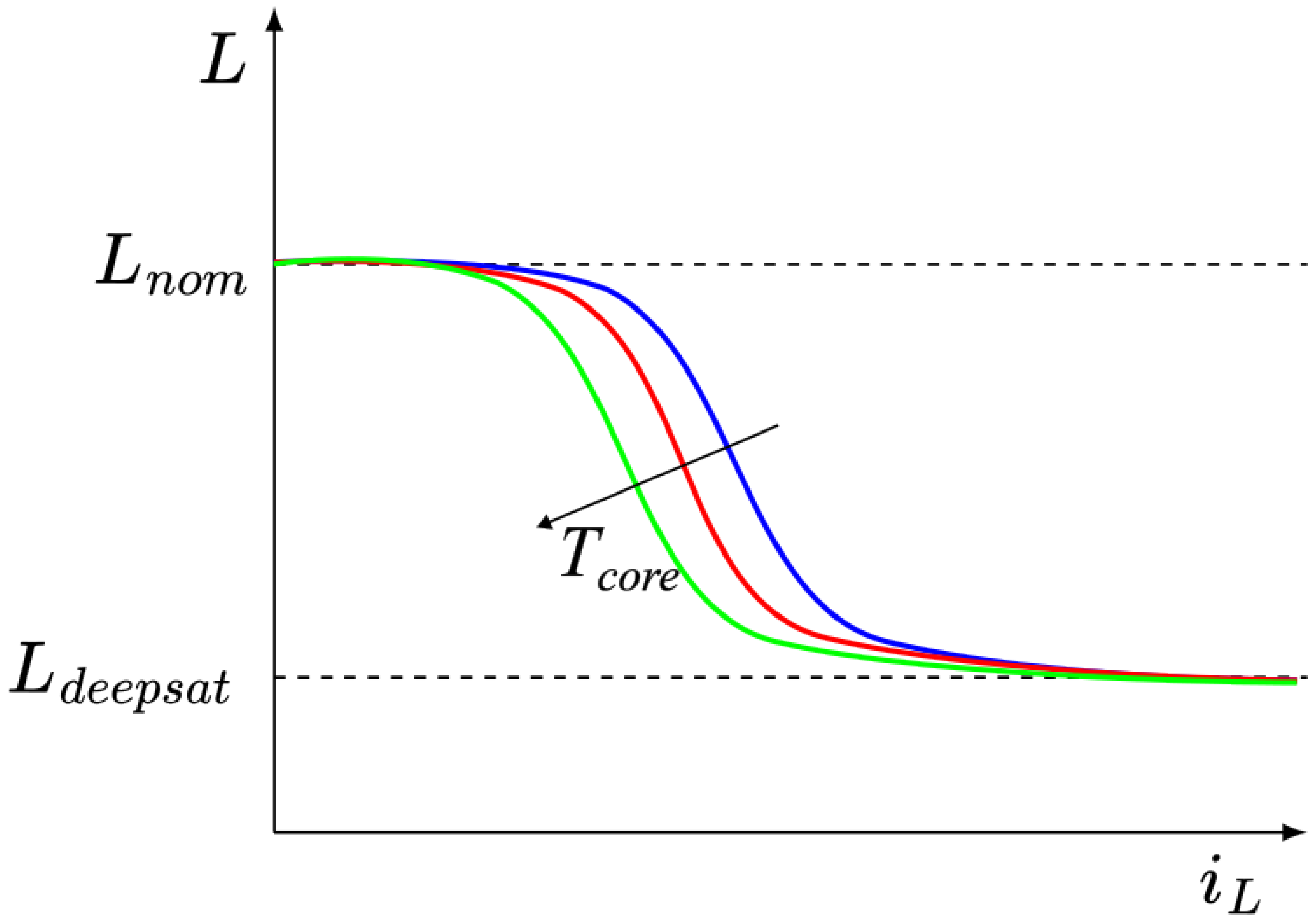
In high power density applications, inductors are often operated beyond their strictly linear region in order to optimize volume and cost [18,21]. Under these conditions, the inductance can no longer be considered constant, but becomes a nonlinear function of both current and temperature, as depicted in Figure 2.

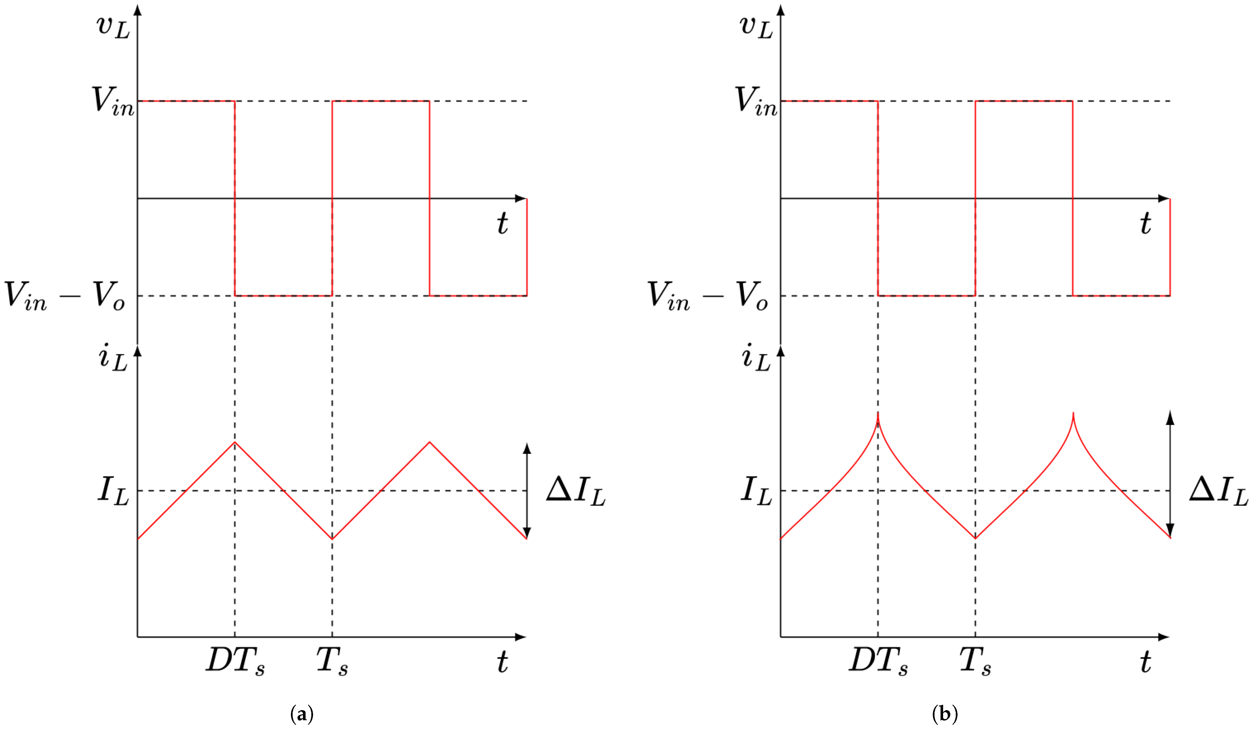
Figure 3 illustrates the typical inductor voltage and current waveforms in a boost converter. In particular, Figure 3a shows the ideal behavior when the inductance remains constant during the switching period, resulting in a linear current ramp. Conversely, Figure 3b highlights the effect of inductance reduction as the current increases, leading to the characteristic cusp-shaped current waveform associated with partial saturation. To accurately characterize this behavior, several mathematical frameworks have been proposed in the literature. Polynomial-based models are widely adopted for their computational efficiency and ability to reproduce the sharp transition into saturation [18,27,28]. Other approaches include arctangent formulations and logistic functions, which excel at capturing deep saturation trends [29,30,31]. Recent research has further expanded these techniques through data-driven methods, such as K-means clustering for temperature estimation and neural network architectures like the E-$\alpha$Net, which capture complex thermal–magnetic dependencies without heavy analytical overhead [30,32].

A significant advancement in the practical exploitation of these components is the Quasi-Constant ON-time (QCOT) control strategy [28]. This method employs a recursive algorithm to dynamically tune the power switch conduction time ($T_{ON}$) based on the real-time temperature and saturation state of the inductor. Studies demonstrate that allowing the inductance to drop to 50% of its nominal value through such control can lead to a 40% increase in operating current and a 70% reduction in component volume compared to traditional linear designs [21,28].

Furthermore, the research by Detka and Górecki on average electrothermal models highlights that accurate knowledge of distributed loss mechanisms is essential for evaluating performance in topologies like boost and SEPIC converters [16,33]. The interaction between temperature-dependent inductance and Joule losses (which increase with temperature due to rising wire resistivity) creates a potential positive feedback loop. This mechanism can trigger thermal runaway.

Under nonlinear operating conditions, the classical ripple expression is no longer valid in its linear form. Any reduction in inductance, whether driven by high DC bias or rising temperature, directly increases the current ripple amplitude and peak current stress. At the same time, copper resistance exhibits an approximately linear temperature dependence; consequently, Joule losses increase with temperature. The combination of temperature-dependent inductance and resistive losses introduces a potential electro–thermal feedback mechanism [18].

An increase in temperature reduces inductance, which in turn increases current ripple and RMS current. This amplifies both copper and magnetic losses, further increasing the temperature. Such nonlinear coupling is particularly critical in boost and buck–boost topologies operating at high duty cycles, where significant DC bias is present.

While classical lumped thermal models (0D) can estimate the average temperature rise, they are inherently limited because they cannot capture spatial temperature gradients, internal hot-spot formation, or the complex transient electro–thermal interactions occurring under realistic dynamic load conditions. These limitations motivate the development of spatially resolved transient thermal models, such as the 1D and 2D approaches presented in the following sections.

In the subsequent section regarding the application (Section 5), a representative cylindrical inductor is analyzed under a prescribed loss partition in order to compare the thermal models under controlled and reproducible assumptions.

3. Analytical Thermal Modeling

This section develops the analytical thermal models for the inductor, which can be simplified as a two-layer composite cylinder: an inner core (Ferrite) and an outer shell (copper winding). Let $R_1$ be the radius of the core and $R_2$ be the outer radius of the winding. The length of the inductor is L. Both materials are assumed to be homogeneous and isotropic. The analysis covers Lumped Parameter (0D), 1D (radial only), and 2D (radial and axial) heat conduction for both steady-state and transient conditions.

3.1. General Governing Equation

The starting point is the transient heat conduction equation (Fourier’s Law with internal generation) in cylindrical coordinates, which expresses the variation in the temperature T with respect to the independent variables $(r,\varphi ,z,t)$. If the component to be analyzed is homogeneous and isotropic, the heat equation can be derived as

$$\rho c_p{\displaystyle \frac{\partial T}{\partial t}}={\displaystyle \frac{1}{r}}{\displaystyle \frac{\partial }{\partial r}}\left(kr{\displaystyle \frac{\partial T}{\partial r}}\right)+{\displaystyle \frac{1}{r^2}}{\displaystyle \frac{\partial }{\partial \phi }}\left(kr{\displaystyle \frac{\partial T}{\partial \phi }}\right)+{\displaystyle \frac{\partial }{\partial z}}\left(k{\displaystyle \frac{\partial T}{\partial z}}\right)+\dot{q},$$

(3)

where $\rho$ is the density (kg m⁻³), $c_p$ is the specific heat capacity (J kg⁻¹ K⁻¹), k is the thermal conductivity (W m⁻¹ K⁻¹), and $\dot{q}$ is the volumetric heat generation rate (W m⁻³). The latter is commonly assumed to be homogeneous within the cylindrical body and constant in time, in order to identify an analytical solution [34].

Due to the geometrical features, in most of the practical cases it is allowed to assume axisymmetric conditions (no dependence on $\phi$) and consider heat flow only in the radial $\left(r\right)$ and axial $\left(z\right)$ directions. Under this assumption, the equation in each domain i (for instance, core or winding) is

$${\rho }_i{c}_{p,i}{\displaystyle \frac{\partial T_i}{\partial t}}={\displaystyle \frac{1}{r}}{\displaystyle \frac{\partial }{\partial r}}\left(k_{i}r{\displaystyle \frac{\partial T_i}{\partial r}}\right)+{\displaystyle \frac{\partial }{\partial z}}\left(k_i{\displaystyle \frac{\partial T_i}{\partial z}}\right)+{\dot{q}}_i,$$

(4)

3.2. 2D Radial–Axial Model (Steady-State and Transient)

This model accounts for heat diffusion in both the radial $\left(r\right)$ and axial $\left(z\right)$ directions and its solution is necessary for accurate hot-spot prediction in most of the practical applications.

3.2.1. 2D Steady-State (Radial–Axial)

The governing equation is

$${\displaystyle \frac{1}{r}}{\displaystyle \frac{\partial }{\partial r}}\left(k_{i}r{\displaystyle \frac{\partial T_i}{\partial r}}\right)+{\displaystyle \frac{\partial }{\partial z}}\left(k_i{\displaystyle \frac{\partial T_i}{\partial z}}\right)+{\dot{q}}_i=0.$$

(5)

The solution employs the superposition principle, assuming that the temperature solution can be found by summing a homogeneous and a particular solution:

$$T_i(r,z)=T_{\mathrm{homogeneous}}(r,z)+T_{\mathrm{particular}}\left(r\right).$$

(6)

In more detail, $T_{\mathrm{homogeneous}}(r,z)$ is the solution of the two-dimensional equation with no internal heat generation, while $T_{\mathrm{particular}}\left(r\right)$ is the solution of the one-dimensional equation with heat conduction over the radial direction only but with internal generation. The homogeneous solution $T_{\mathrm{homogeneous}}$ is found via separation of variables, expressing the temperature as the product of a radial function $R\left(r\right)$ and axial function $Z\left(z\right)$, $T(r,z)=R\left(r\right)·Z\left(z\right)$.

$R\left(r\right)$ is given by the sum of zero-th order Bessel functions $J_0(\beta ·r)$ and $Y_0(\beta ·r)$, while $Z\left(z\right)$ is given by the sum of hyperbolic functions $sinh(\beta ·z)$ and $cosh(\beta ·z)$ [35].

The solution of this equation was applied in [36] for an electrolytic capacitor modeled as a single-layer cylinder. Since the capacitor is mounted vertically, the boundary conditions assume that the mounting base is thermally insulated and that the other base and the lateral surface undergo a convection heat transfer. The other boundary conditions assume that the temperature peak value in the radial direction occurs in the cylinder axis, that the temperature peak value in the axial direction occurs at half height, and that the external surfaces dissipate the excess thermal power through convective heat transmission.

Considering these boundary conditions, the solution found from these authors is

$$\theta (r,z)={\displaystyle \frac{\dot{q}{R}_1^2}{4k}}\left(1-{\displaystyle \frac{r^2}{R_1^2}}\right)+{\displaystyle \frac{\dot{q}{R}_1}{h(2+R_1/L)}}+\sum _{n=1}^{\infty }{C}_{n}cosh\left({\beta }_{n}z\right)J_0\left({\beta }_{n}r\right),$$

(7)

where $R_1$ is the capacitor outer radius, L is the capacitor length, h is the convection heat transfer coefficient, $\beta$ are some of the integration constants, and $C_n$ are the other integration constants, given by the following expression:

$$C_n={\displaystyle \frac{\frac{h\dot{q}{R}_{1}Bi}{k^2{\beta }_n{J}_1\left({\lambda }_n\right)}-\frac{2\dot{q}B{i}^2}{{\beta }_n{J}_1\left({\lambda }_n\right)k(2+R_1/L)}-\frac{2h\dot{q}B{i}^2}{{\beta }_n^3{R}_1{k}^2{J}_1\left({\lambda }_n\right)}}{[{\beta }_{n}sinh\left({\beta }_{n}L\right)+hcosh\left({\beta }_{n}L\right)/k][B{i}^2+{\lambda }_n^2]}},$$

(8)

where $Bi$ is the Biot number [37].

Floris et al. [36] found that the solution converges after $n=30$, stating that even a modern hand calculator could handle this computational burden. Moreover, they compared this analytical solution against a FE model. Although an estimation of the error between these two methods was not provided, the authors show two different figures with the results of the two methods, concluding that the analytical exact solution with constant properties is quite close to the FEM solution, with the advantage of requiring much shorter time.

3.2.2. 2D Transient (Radial–Axial)

The full transient heat equation in two dimensions is

$${\rho }_i{C}_{p,i}{\displaystyle \frac{\partial T_i}{\partial t}}={\displaystyle \frac{1}{r}}{\displaystyle \frac{\partial }{\partial r}}\left(k_{i}r{\displaystyle \frac{\partial T_i}{\partial r}}\right)+{\displaystyle \frac{\partial }{\partial z}}\left(k_i{\displaystyle \frac{\partial T_i}{\partial z}}\right)+{\dot{q}}_i.$$

(9)

The solution is obtained by extending the separation of variables method in all three dimensions $(r,z,t)$:

$$T_i(r,z,t)=T_{i,ss}(r,z)+\sum _{m=1}^{\infty }\sum _{n=1}^{\infty }{A}_{m,n}{R}_m\left(r\right)Z_n\left(z\right)e^{-({\lambda }_m^2+{\mu }_n^2){\alpha }_{i}t}.$$

(10)

In addition to the boundary conditions, the coefficients $A_{m,n}$ should be determined from the initial condition $T(r,z,0)=T_0$ using the orthogonality properties of the radial and axial eigenfunctions in the two-layer composite domain [35]. The analytical solution for 2D cylindrical shells with periodical boundary conditions but without internal generation was found in [38], while the 3D problem of cylindrical shells with thermal power generation was solved in [39].

To the best of the authors’ knowledge, this kind of modeling approach was never applied in power electronics components.

3.3. 1D Radial Model (Steady-State and Transient)

This model simplifies the problem by assuming the heat flow is purely radial, thus neglecting axial conduction (${\displaystyle \frac{\partial }{\partial z}}=0$).

3.3.1. 1D Steady-State (Radial)

The governing equation is derived by setting ${\displaystyle \frac{\partial }{\partial t}}=0$:

$${\displaystyle \frac{1}{r}}{\displaystyle \frac{d}{dr}}\left(k_{i}r{\displaystyle \frac{d{T}_i}{dr}}\right)+{\dot{q}}_i=0.$$

(11)

This is a first order, linear, non-homogeneous differential equation, whose general solution for each i-th layer is

$$T_{i,ss}\left(r\right)=-{\displaystyle \frac{{\dot{q}}_i}{4k_i}}{r}^2+C_{1,i}ln\left(r\right)+C_{2,i}.$$

(12)

The constants $C_{1,i}$ and $C_{2,i}$ are commonly determined by two conditions for each body. Considering an inductor with core and winding (two bodies), with $R_1$ being the external core radius and $R_2$ the external winding radius, the following four boundary/interface conditions are commonly set:

• $r=0$ (Symmetry): ${\displaystyle \frac{d{T}_{\mathrm{core}}}{dr}}=0$.
• $r=R_1$ (Temperature continuity): $T_{\mathrm{core}}\left(R_1\right)=T_{\mathrm{winding}}\left(R_1\right)$.
• $r=R_1$ (Flux continuity): $k_{\mathrm{core}}{\displaystyle \frac{d{T}_{\mathrm{core}}}{dr}}{|}_{R_1}=k_{\mathrm{winding}}{\displaystyle \frac{d{T}_{\mathrm{winding}}}{dr}}{|}_{R_1}$.
• $r=R_2$ (Convection): $-k_{\mathrm{winding}}{\displaystyle \frac{d{T}_{\mathrm{winding}}}{dr}}{|}_{R_2}=h[T_{\mathrm{winding}}\left(R_2\right)-T_{\infty }]$.

where $T_{\infty }$ is the temperature of the air surrounding the winding, which dissipate its thermal power with a convective coefficient h.

This approach was used by Parler [40] for an electrolytic capacitor, obtaining an optimal agreement with experimental measurements.

3.3.2. 1D Transient (Radial)

The governing equation is

$${\rho }_i{c}_{p,i}{\displaystyle \frac{\partial T_i}{\partial t}}={\displaystyle \frac{1}{r}}{\displaystyle \frac{\partial }{\partial r}}\left(k_{i}r{\displaystyle \frac{\partial T_i}{\partial r}}\right)+{\dot{q}}_i.$$

(13)

Since this is a non-homogeneous equation, the separation of variables method is not applicable. Nevertheless, since it is a linear equation, it is possible to solve it resorting to the superposition principle, solving a single variable, non-homogeneous transient equation, and a two-variables, steady-state homogeneous equation separately. The transient equation is then solved through the separation of variables method, splitting the temperature in the product of two functions depending on a single variable, $T(r,t)=R\left(r\right)\Gamma \left(t\right)$. The solution to this method gives the result that the spatial dependency involves Bessel functions of the first and second kind ($J_0$ and $Y_0$), while the temporal solution is exponential:

$$T_{i,trans}(r,t)=T_{i,ss}\left(r\right)+\sum _{n=1}^{\infty }{A}_n{R}_n\left(r\right)e^{-{\lambda }_n^2{\alpha }_{i}t},$$

(14)

where $T_{i,ss}\left(r\right)$ is the steady-state solution, ${\alpha }_i=k_i/\left({\rho }_i{c}_{p,i}\right)$ is the thermal diffusivity, and the eigenvalues ${\lambda }_n$ are obtained from the boundary and interface conditions.

3.4. Lumped Parameter Models (0D)

This category of models, represented by a simple thermal resistance–capacitance network, provides the fastest prediction of the average temperature rise ($\Delta T_{avg}$) but neglects internal gradients. It is used when a single-body analysis is allowed.

3.4.1. 0D Transient: Governing Equation (Thermal–Electrical Analogy)

The total heat generated ($P_{loss}$) is balanced by the heat stored ($C_{th}$) and the heat dissipated to the ambient ($R_{th,total}$):

$$P_{loss}=C_{th}{\displaystyle \frac{d(\Delta T_{avg})}{dt}}+{\displaystyle \frac{\Delta T_{avg}}{R_{th,total}}}.$$

(15)

3.4.2. Thermal Resistances Approach

The thermal resistance approach can be formalized following the electro–thermal framework proposed in [18] and deepened experimentally in [26]. In this representation, the inductor is modeled as a first-order thermal system characterized by a global thermal resistance ($R_{th}$) toward the ambient and a thermal capacitance ($C_{th}$), leading to the thermal time constant

$${\tau }_{th}=R_{th}{C}_{th}$$

(16)

The temperature rise of the core is governed by the following energy balance equation:

$$C_{th}{\displaystyle \frac{d{T}_{core}}{dt}}=P_{loss}-{\displaystyle \frac{T_{core}-T_{\infty }}{R_{th}}}$$

(17)

Under steady-state conditions, the relationship simplifies to

$$T_{core}-T_{\infty }=P_{loss}{R}_{th}$$

(18)

where $P_{loss}$ accounts for the total heat generated from both Joule losses and magnetic losses [18,21]. As established in the literature, the inductor is represented through an electrical–thermal analogy where temperature corresponds to voltage, heat flow to current, and thermal resistance to electrical resistance [18], as depicted in Figure 4.

This compact representation enables the coupling between electrical and thermal domains. Specifically, when the inductor operates in partial saturation, the losses become temperature-dependent. An increase in temperature reduces the inductance, which consequently increases current ripple and peak current, further escalating Joule losses [26]. This positive feedback mechanism has been analytically derived, where the thermal stability condition is expressed as

$$k_1{k}_2>-{\displaystyle \frac{1}{R_{th}}}$$

(19)

where $k_1$ gives the Joule losses dissipated within the inductor and $k_2$ represents the inductance sensitivity from the core temperature. This condition highlights that the thermal resistance plays a crucial role in defining the safe operating region of the converter when the inductor is exploited under nonlinear operating regimes [26].

3.4.3. Transient Equation Solution

Assuming a constant $P_{loss}$ applied at $t=0$, the transient temperature rise is

$$\Delta T_{avg}\left(t\right)=R_{th,total}{P}_{loss}\left(1-e^{-t/{\tau }_{th}}\right),$$

(20)

where the thermal time constant is ${\tau }_{th}=R_{th,total}{C}_{th}$. The total thermal capacitance is $C_{th}={\sum }_i\left({\rho }_i{C}_{p,i}{V}_i\right)$.

This solution can be found in Ref. [41], where it was applied to a series of thermal resistances taking into account natural convection and radiation from the capacitor to the environment, and the internal conduction heat transfer.Simulation results were later compared with measurements in transient conditions, obtaining a very good prediction, with deviations always below 10%.

3.4.4. Second Order (Two Bodies) Lumped Parameter

When the body is thick or the temperatures of core and windings should be analyzed separately, the lumped parameters approach can be exploited considering two bodies thermally interacting with each other and the surrounding environment [42]. With this approach, a common inductor can be modeled as a cylindrical core surrounded by the windings, where heat generation for hysteresis and eddy current losses occur in the core while losses for Joule effect occur in the windings.

Under these conditions, we can write

$${\displaystyle \frac{\partial }{\partial t}}\left[{\left(\rho vc\right)}_{core}{T}_{core}(r,t)\right]={\dot{q}}_{core}\left(T_{core}\right)v_{core}-q_{core-wind}^{″}(T_{wind},T_{core})S_{core},$$

(21)

$${\displaystyle \frac{\partial }{\partial t}}\left[{\left(\rho vc\right)}_{wind}{T}_{wind}(r,t)\right]={\dot{q}}_{wind}{v}_{wind}+q_{core-wind}^{″}(T_{wind},T_{core})S_{core}-h_o{S}_o\left[T_{wind}(S_o,t)-T_{\infty }\right],$$

(22)

where $q_{core-wind}^{″}$ is the heat conduction exchange between the two bodies, $S_{core}$ is the external core surface, i.e., the heat conduction exchange area, and $S_o$ is the outer surface of the electronic component, i.e., the heat convection exchange area.

Through the lumped parameters method, the spatial distribution of the temperature is neglected and the derivatives become total. The solution method proposed in [42] lies in expressing the heat flow between inner and outer shells through a specific resistance $h_c$. The system becomes

$${\displaystyle \frac{d}{dt}}\left[{\left(\rho vc\right)}_{core}{T}_{core}\left(t\right)\right]={\dot{q}}_{core}{v}_{core}-h_c{S}_{core}(T_{core}-T_{wind}),$$

(23)

$${\displaystyle \frac{d}{dt}}\left[{\left(\rho vc\right)}_{wind}{T}_{wind}\left(t\right)\right]={\dot{q}}_{wind}{v}_{wind}+h_c{S}_{core}(T_{core}-T_{wind})-h_o{S}_o\left[T_{wind}-T_{\infty }\right],$$

(24)

Additionally, the two time constants of the problem and other parameters are defined:

$${\tau }_1={\displaystyle \frac{{\left(\rho cv\right)}_{core}}{h_c{S}_{core}}};{\tau }_2={\displaystyle \frac{{\left(\rho cv\right)}_{wind}}{h_o{S}_o}};b={\displaystyle \frac{1}{{\tau }_1}}+{\displaystyle \frac{1}{{\tau }_2}}+{\displaystyle \frac{h_c{S}_{core}}{h_o{S}_o{\tau }_2}};c={\displaystyle \frac{1}{{\tau }_1{\tau }_2}}$$

(25)

The solution of the system of differential equations is

$$T_{core}=T_{\infty }+{\displaystyle \frac{{\dot{q}}_{core}{v}_{core}}{h_c{S}_{core}}}+{\displaystyle \frac{{\dot{q}}_{core}{v}_{core}+{\dot{q}}_{wind}{v}_{wind}}{h_o{S}_o}}+C_1{e}^{\left[-{\displaystyle \frac{b}{2}}+\sqrt{{\left({\displaystyle \frac{b}{2}}\right)}^2-c}\right]t}+C_2{e}^{\left[-{\displaystyle \frac{b}{2}}-\sqrt{{\left({\displaystyle \frac{b}{2}}\right)}^2-c}\right]t},$$

(26)

$$T_{wind}=T_{\infty }+{\displaystyle \frac{{\dot{q}}_{core}{v}_{core}+{\dot{q}}_{wind}{v}_{wind}}{h_o{S}_o}}+C_1^{\prime }{e}^{\left[-{\displaystyle \frac{b}{2}}+\sqrt{{\left({\displaystyle \frac{b}{2}}\right)}^2-c}\right]t}+C_2^{\prime }{e}^{\left[-{\displaystyle \frac{b}{2}}-\sqrt{{\left({\displaystyle \frac{b}{2}}\right)}^2-c}\right]t}.$$

(27)

The integration constants $C_1$ and $C_2$ can be found by setting the initial conditions.

The approach of separately assessing two temperatures was employed in [21], where the lumped approach hypothesis was applied only for the windings, keeping the spatial resolution only for the core. In this study, Equation (24) was replaced with the following:

$${\displaystyle \frac{d}{dt}}\left[{\left(\rho vc\right)}_{wind}{T}_{wind}\left(t\right)\right]={\dot{q}}_{wind}{v}_{wind}+q_{core-wind}^{″}(T_{wind},T_{core})S_{core}-h_o{S}_o\left[T_{wind}\left(t\right)-T_{\infty }\right],$$

(28)

Since the authors did not find an analytical solution to this system in transient conditions but only in steady-state, they resorted to the thermal resistances method. The transient problem was then solved via a numerical method, where the dependency of losses (Joule, hysteresis, and eddy currents) from the temperature was also taken into account.

3.5. Anisotropic Models

The general heat equation can be reformulated to take into account the anisotropies within the body, with respect to different values of thermal conductivity over the different directions.

$${\displaystyle \frac{k_{\theta }}{r^2}}{\displaystyle \frac{{\partial }^{2}T}{\partial {\theta }^2}}+{\displaystyle \frac{k_r}{r}}{\displaystyle \frac{\partial }{\partial r}}\left(r{\displaystyle \frac{\partial T}{\partial r}}\right)+k_z{\displaystyle \frac{{\partial }^{2}T}{\partial z^2}}+Q=\rho c_p{\displaystyle \frac{\partial T}{\partial t}}$$

(29)

Some studies related to the thermal analysis of anisotropic cylinders also found analytical solutions [43,44,45,46].

For instance, Sarkar et al. [44] found that, for a cylinder of height H in steady-state conditions, the temperature solution is

$$T(r,\theta ,z)=w(r,\theta ,z)+f\left(z\right),$$

(30)

where

$$w(r,\theta ,z)=\sum _{m=0}^{\infty }\sum _{n=1}^{\infty }{C}_{m.n}·I_{\nu ,m}\left({\eta }_n\sqrt{{\displaystyle \frac{k_z}{k_r}}}r\right)cos\left(m\theta \right)\left[{\displaystyle \frac{h_{end}}{{\eta }_n{k}_z}}sin\left({\eta }_{n}z\right)+cos\left({\eta }_{n}z\right)\right].$$

(31)

and

$$f\left(z\right)={\displaystyle \frac{Q·H^2}{2k_z}}\left[{\displaystyle \frac{z}{H}}\left(1-{\displaystyle \frac{z}{H}}\right)+{\displaystyle \frac{k_z}{h_{end}·H}}\right],$$

(32)

Moreover, an exact analytical solution in composite cylindrical shells for anisotropic non-axisymmetric heat conduction was derived by Norouzi et al. in steady-state conditions [45] and by Rahmani et al. in transient conditions [46].

These approach were, nevertheless, not oriented to solve the thermal problem of electronic components.

3.6. Summary of Thermal Modeling Approaches

Table 1. Summary of main features of analytical thermal modeling approaches.

Model	Domain	Temperature Result	Advantages	Disadvantages
Lumped (0D) Transient	$\Delta T_{avg}\left(t\right)$	Average over time	Maximum computational speed; simplicity.	Ignores all internal gradients and hot-spots.
1D Radial Steady-State	$T\left(r\right)$	Radial gradient	Fast; includes radial conduction effects.	Ignores axial (z) flow; no time dependence.
1D Radial Transient	$T(r,t)$	Radial gradient over time	Captures thermal time constant and internal r dynamics.	Ignores axial (z) heat spreading (less accurate for short components).
2D Radial–Axial Steady-State	$T(r,z)$	Full spatial temperature field	Accurate hot-spot and heat spreading prediction at ∞.	More complex mathematical solution (Bessel functions).
2D Radial–Axial Transient	$T(r,z,t)$	Full $r,z$ dynamics over time	Highest spatial accuracy under axisymmetric assumptions; suitable for fast electro–thermal co-simulation.	Most complex mathematically; requires double infinite series summation.

illustrates a summary of the main characteristics of the proposed analytical models, while

Table 2. Summary of Analytical thermal modeling approaches of electronic components.

Ref.	Space Description	Time Description	Internal Generation	Anisotropy	Convective Coefficient
[41]	0D (resistance)	Steady-state	No	No	Calculated with correlation
[40]	1D	Steady-state	Yes	Yes	Calculated with correlation
[22]	1D	Transient	Yes	No	Sensitivity analysis
[21]	1D	Transient	Yes	No	Sensitivity analysis
[36]	2D	Steady-state	Yes	No	Calculated with correlation

compares the main modeling approaches adopted by the authors of the existing scientific literature.

4. Thermal Modeling of External Heat Flow

Heat dissipation from the electronic component to the surrounding environment can occur through the three simple modes of heat transfer: conduction, convection, and radiation. Conduction is a bulk heat transfer mechanism that depends on both the geometry of the heat path and the effective cross-sectional area, and it becomes relevant mainly when the electronic component is surrounded or linked to a heat sink. In contrast, convection is typically treated as a surface-driven process: although the thermal interaction originates at the surface, the associated velocity and temperature fields in the adjacent fluid extend into a boundary layer. The effectiveness of convective heat exchange between a solid surface, such as the external surface of the component, and the surrounding fluid (e.g., air) is quantified by the convective heat transfer coefficient h, which is strongly influenced by the fluid flow conditions and by transport properties such as density and viscosity. Convection also strongly depends on the fluid velocity, which can originate from buoyancy forces, related to the dependence of the fluid density from the temperature, or from an external device (e.g., a fan). The different origin of the fluid motion classifies convection into natural or forced. Radiative heat transfer, as well as convection, occurs as an exchange between a surface and its surrounding environment. Its magnitude depends not simply on the temperature difference between the surface and the surrounding environment but on the fourth power of the absolute temperature levels of both. In addition, the effectiveness of radiative exchange is strongly influenced by the surface emissivity $\epsilon$, which characterizes how efficiently the surface emits thermal radiation. Nevertheless, this phenomenon is often linearized resorting to a temperature-dependent radiation coefficient $h_{rad}$. According to [40], for electrolytic capacitors with approximately a 2.5” diameter and 5” winding in environment air temperature, the radiation coefficient varies between 5 and 9 W/(m² K), while the natural convection coefficient varies between 5 and 7 W/(m² K), making these phenomena comparable with each other.

An easy-to-use formula to estimate the global heat transfer coefficient based on the air speed $v_a$ only, thus including forced convection, natural convection, and radiation, was referenced by Parler and also used by Floris et al. [36]:

$$h_{TOT}=11\sqrt{{\displaystyle \frac{(v_a+0.25)}{0.25}}}=11\sqrt{4v_a+1}\left[{\mathrm{W}/\mathrm{m}}^2\mathrm{K}\right],$$

(33)

where the air speed is expressed in SI units.

The same author shows more detailed formulas for natural convection only and forced convection only. A comprehensive formula for forced convection, known as Churchill–Bernstein heat transfer correlation [47,48], can be used for any cylindrical object in cross-flow, which relates to the following non-dimensional numbers:

$$Re={\displaystyle \frac{\rho v_{a}D}{\mu }};Pr={\displaystyle \frac{\mu c_p}{k}},$$

(34)

$$Nu={\displaystyle \frac{hD}{k}}=0.3+{\displaystyle \frac{0.62R{e}^{1/2}P{r}^{1/3}}{{[1+{(0.4/Pr)}^{2/3}]}^{1/4}}}{\left[1+{\left({\displaystyle \frac{Re}{282,000}}\right)}^{5/8}\right]}^{4/5},$$

(35)

that are valid over a wide range of values, until $RePr>0.2$, with all properties evaluated at the film temperature. It is worth highlighting that the coefficient shown by Parler is 28,200, rather than 282,000.

The natural convection coefficient can easily be calculated, according to [40], with respect to the temperature difference $\Delta T$ (in °C or K) and the diameter D (in m) with

$$h=1.32{\left({\displaystyle \frac{\Delta T}{D}}\right)}^{1/4}\left[{\mathrm{W}/\mathrm{m}}^2\mathrm{K}\right].$$

(36)

For natural convection of vertical cylindrical capacitors with radial direction flow, Freiburger [41] used the Churchill–Chu correlation [48,49]:

$$Nu={\left[0.825+{\displaystyle \frac{0.387R{a}_L^{1/6}}{{[1+{(0.492/Pr)}^{9/16}]}^{8/27}}}\right]}^2,$$

(37)

where $Ra$ is the Rayleigh number and $R{a}_L$ means that it should be evaluated with respect to the cylinder length L. This correlation can be used when the following condition is satisfied:

$${\displaystyle \frac{D}{L}}>{\displaystyle \frac{35}{G{r}_L^{1/4}}},$$

(38)

with $G{r}_L$ being the Grashof number evaluated with respect to the cylinder length L.

Last, Churchill and Chu have recommended the following correlation for natural convection of horizontal cylinders, valid for a wide Rayleigh number range [48]:

$$Nu={\left[0.60+{\displaystyle \frac{0.387R{a}_D^{1/6}}{{[1+{(0.559/Pr)}^{9/16}]}^{8/27}}}\right]}^2.$$

(39)

5. Application

This section applies the modeling approaches derived in Section 3 to a representative cylindrical inductor, to (i) provide a reproducible workflow for model setup, (ii) compare the temperature predictions obtained with lumped (0D), radial (1D), and radial–axial (2D) formulations under the same loss and cooling assumptions, and (iii) quantify the accuracy gain versus the additional computational cost.

Before comparing the 0D, 1D, and 2D benchmark cases, an experimental validation was carried out in order to assess the ability of the proposed framework to reproduce the measured external thermal response of a practical power inductor.

5.1. Experimental Validation

The experimental setup consists of a DC-DC boost converter prototype instrumented for simultaneous electrical and thermal acquisition; the converter is equipped with a custom-made inductor made of a ferrite core (diameter of 1 cm) and a copper winding (one layer with copper diameter of 1 mm), with a nominal inductance $L=1$ mH. The objective of this section is not to reconstruct the full internal temperature field, which is not directly accessible experimentally, but to validate the predicted external thermal response and the dominant heating transient under realistic converter operation.

The boost converter includes a FDP12N60NZ MOSFET and a MURB820 diode; the main electrical characteristics are summarized in

Table 3. Operating conditions adopted for the experimental validation.

Quantity	Symbol	Value
Input voltage	$V_{in}$	20 V
Duty cycle	D	50
Switching frequency	$f_s$	100 kHz
Output load	$R_L$	20 $\Omega$
Output capacitor	C	33 $\mathsf{\mu }$F
Nominal inductance	L	1 mH

. The setup is composed of a oscilloscope MS2024B from Tektronix (Beaverton, OR, USA), HQPower DC power supply PS23023, and a thermo-camera SC660 from FLIR (Wilsonville, OR, USA).

During the experiment, the winding surface temperature was recorded over time from startup up to quasi-steady-state conditions. In parallel, the electrical quantities required to define the operating point were acquired from the converter waveforms.

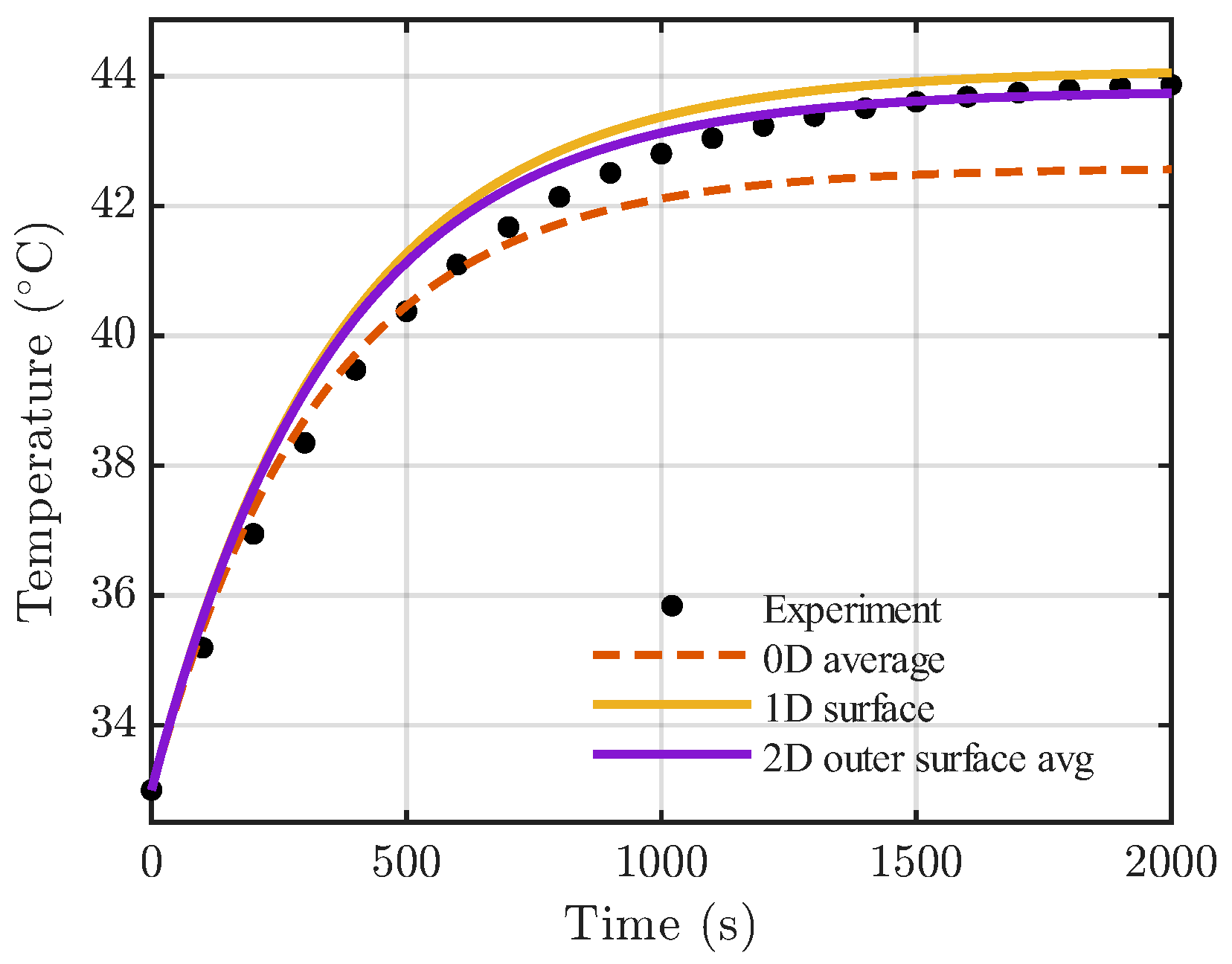
For validation, the model prediction was compared against the measured winding surface temperature in both transient and quasi-steady-state conditions. Since the available measurement concerns an externally accessible thermal quantity, the comparison was performed against the 1D surface temperature prediction and against the 2D outer lateral surface average temperature. The 0D model was also retained in the comparison as a reference for the average thermal behavior.

The agreement was quantified through the Relative Root Mean Square Error percentage (RRMSE%), defined as

$$\mathrm{RRMSE}\%=\sqrt{{\displaystyle \frac{{\sum }_{i=1}^N{(x_i-y_i)}^2}{{\sum }_{i=1}^N{y}_i^2}}}·100,$$

(40)

where $x_i$ and $y_i$ denote the analytical and experimental temperature samples, respectively, and N is the number of acquired data points.

Figure 5 compares the measured winding surface temperature transient with the predictions of the 0D, 1D, and 2D models. The 1D and 2D formulations both reproduce the measured external thermal response with high accuracy, while the 2D model provides the closest agreement over the whole transient. In contrast, the 0D model correctly captures the dominant heating dynamics, but systematically underestimates the measured external temperature because of its lumped nature.

The corresponding quantitative metrics are reported in

Table 4. Quantitative comparison between experimental and modeled temperature transients.

Model	RRMSE%	Final Error [°C]	Final Error on $\mathbf{\Delta }\mathit{T}$ [%]
0D average	19.6	1.307	12.02
1D surface	13.8	0.182	1.67
2D outer surface average	10.6	0.133	1.22

. The 2D model achieves the lowest error, with an RRMSE% of 10.6% and a final quasi-steady-state error of 0.133 °C, followed closely by the 1D model, with an RRMSE% of 13.8% and a final error of 0.182 °C. The 0D model remains acceptable in terms of global thermal dynamics, but shows a larger final deviation of 1.307 °C.

It should be emphasized that the experimental validation presented here is based on externally accessible thermal quantities, namely the winding surface temperature evolution measured during converter operation. As a consequence, the comparison directly validates the predicted outer thermal response and the dominant transient behavior, whereas the internal temperature field and the actual core hot-spot cannot be accessed experimentally in the present setup. Therefore, the internal temperature distribution discussed in the following subsections retains a model-based character, consistent with the adopted geometry, boundary conditions, and loss partition assumptions.

Once the framework is validated against the measured outer-temperature response, the benchmark comparison among the 0D, 1D, and 2D formulations is carried out in the following subsections under controlled and reproducible conditions.

5.2. Case Study Definition and Comparison Metrics

The benchmark cases discussed below are introduced after the experimental validation in order to compare the 0D, 1D, and 2D thermal formulations under controlled assumptions. In this second step, the objective is not to reproduce a single measured operating point, but to establish a consistent analytical comparison among models of different spatial complexity using prescribed geometry, losses, and boundary conditions.

The benchmark considered in this work is based on two families of cylindrical inductors modeled as two-layer composite bodies, composed of an inner ferrite core ($0\le r\le R_1$) and an outer copper winding region ($R_1\le r\le R_2$), with axial length L. Axisymmetric conditions are assumed, consistently with Equation (4), and the thermophysical properties of each region are considered constant.

The first family corresponds to a geometry with $R_1=5$ mm and $R_2=6$ mm, already representative of compact winding-dominated inductors. The second family corresponds to a larger-radius geometry, here introduced to emphasize the role of axial heat spreading and end-face cooling, with $R_1=30$ mm and $R_2=32$ mm. For both families, two axial lengths are considered, namely $L=50$ mm and $L=200$ mm.

Uniform volumetric heat generation is prescribed in each domain through ${\dot{q}}_{core}$ and ${\dot{q}}_{wind}$. This assumption is intentionally adopted to isolate the effect of thermal model order and to establish a reproducible benchmark case under controlled conditions. The total dissipated power is fixed to $P_{loss}=5$ W, partitioned as $P_{core}=0.01P_{loss}$ and $P_{wind}=0.99P_{loss}$, consistently with winding-dominated operating conditions.

At the symmetry axis ($r=0$), zero radial heat flux is imposed. At the core-winding interface ($r=R_1$), both temperature continuity and heat-flux continuity are enforced. At the external cylindrical surface ($r=R_2$), heat is dissipated toward ambient air at temperature $T_{\infty }$ through convection with coefficient h. In the 2D model, convection is also applied on both end faces ($z=0$ and $z=L$), while the 1D formulation neglects axial heat spreading and therefore does not represent end-face cooling.

For the benchmark application, the ambient temperature is fixed to $T_{\infty }=40°\mathrm{C}$ and the convection coefficient is set to $h=10$ W/(m²K), representative of simplified natural-air cooling conditions.

Three modeling levels are compared under identical thermal inputs: (a) a 0D lumped transient model, which predicts the average temperature rise; (b) a 1D radial model, which resolves radial temperature profiles in steady-state and transient conditions; and (c) a 2D radial–axial model, which accounts for both axial heat spreading and end-face cooling.

To compare the models consistently, the following quantities are extracted:

• Hot-spot temperature $T_{HS}\left(t\right)={max}_{r,z}T(r,z,t)$ for the 2D model and its 1D counterpart $T_{HS,1D}\left(t\right)={max}_{r}T(r,t)$.
• Spatially averaged temperature $\overline{T}\left(t\right)$, used to enable a consistent comparison with 0D predictions.
• Axial gradient indicator $\Delta T_z\left(t\right)=T(r^{★},z=L/2,t)-{\displaystyle \frac{1}{2}}\left[T(r^{★},0,t)+T(r^{★},L,t)\right]$, where $r^{★}$ is chosen at the predicted hot-spot radius.

The main benchmark parameters are summarized in

Table 5. Main benchmark parameters for the two geometric families considered in the application section.

Parameter	Symbol	Value
Axial length	L	50 mm & 200 mm
Geometry core radius	$R_1$	5.0 mm & 30.0 mm
Geometry outer radius	$R_2$	6.0 mm & 32.0 mm
Ambient temperature	$T_{\infty }$	40 °C
Convection coefficient	h	10 W/(m2K)
Total losses	$P_{loss}$	5 W
Core losses	$P_{core}$	0.05 W
Winding losses	$P_{wind}$	4.95 W

.

5.3. First Benchmark: Small-Radius Cylindrical Inductor

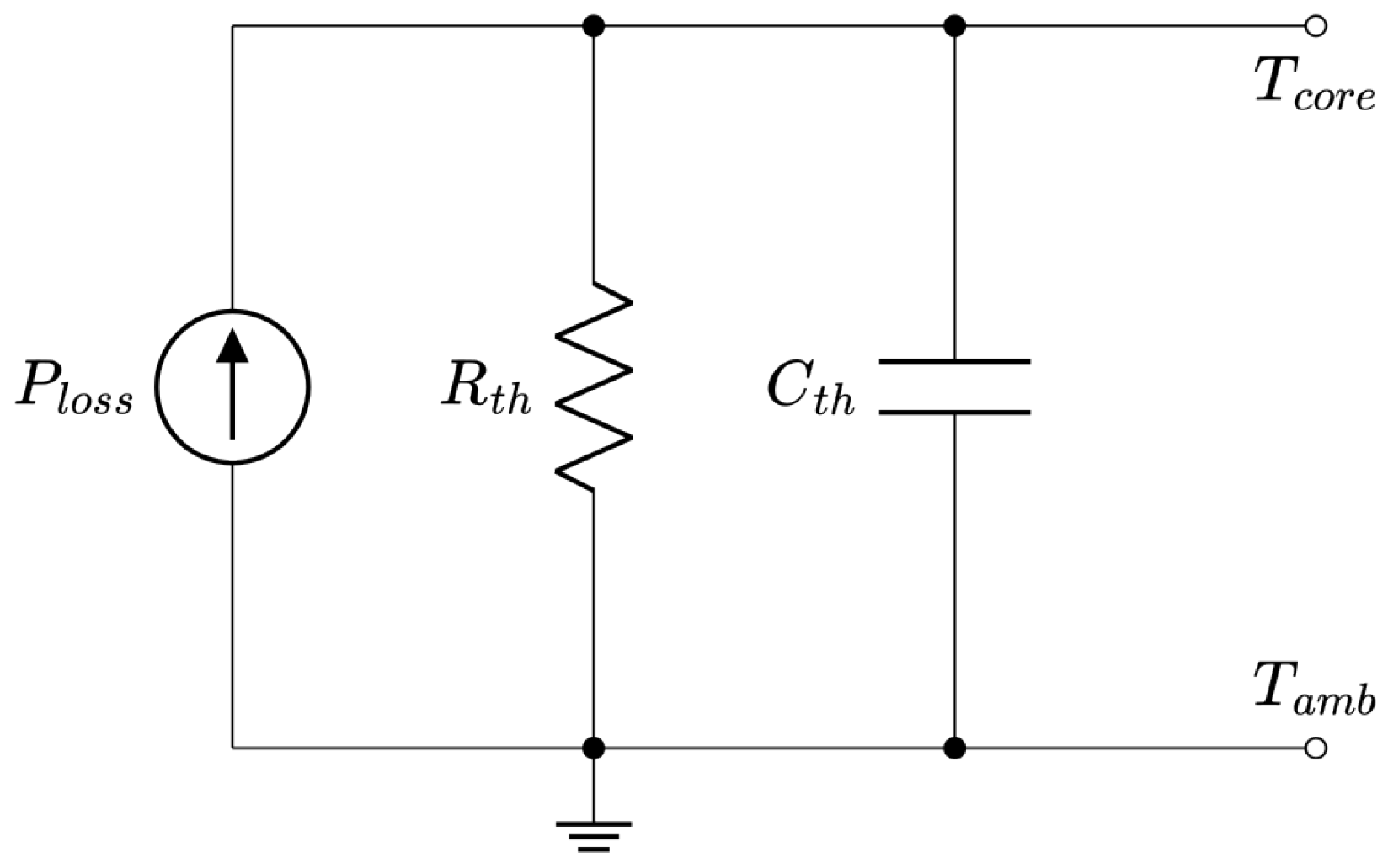
As a baseline comparison, the inductor is first modeled as a single lumped thermal body characterized by a global thermal resistance $R_{th}$ toward the environment and an equivalent thermal capacitance $C_{th}$. Under this assumption, spatial temperature gradients inside the component are neglected and the entire structure is described by a uniform average temperature. Mathematically, the validity of lumped approach is expressed as a Biot number lower than 0.1, which is verified with this geometry.

Under these assumptions, the equivalent thermal resistance is

$$R_{\theta }={\displaystyle \frac{1}{h{A}_{out}}},$$

(41)

where $A_{out}=2\pi R_{2}L+2\pi R_2^2$ is the total external exchange area. The overall thermal capacitance is

$$C_{\mathrm{tot}}=\sum _i{m}_i{c}_{p,i},$$

(42)

including both ferrite and copper contributions. The transient response is therefore governed by a first-order system:

$$T\left(t\right)=T_{\infty }+\left(T_{\mathrm{ss}}-T_{\infty }\right)\left(1-e^{-t/\tau }\right),$$

(43)

with time constant $\tau =R_{\theta }{C}_{tot}$.

Table 6. Thermal 0D simulation results for the two inductor lengths.

Quantity	Symbol	$\mathit{L}=50$ mm	$\mathit{L}=200$ mm
Equivalent thermal resistance	$R_{\theta }$	$47.37$ K/W	$12.88$ K/W
Total thermal capacitance	$C_{tot}$	$71.7$ J/K	$286.8$ J/K
Thermal time constant	$\tau$	3396 s ($56.6$ min)	3693 s ($61.6$ min)
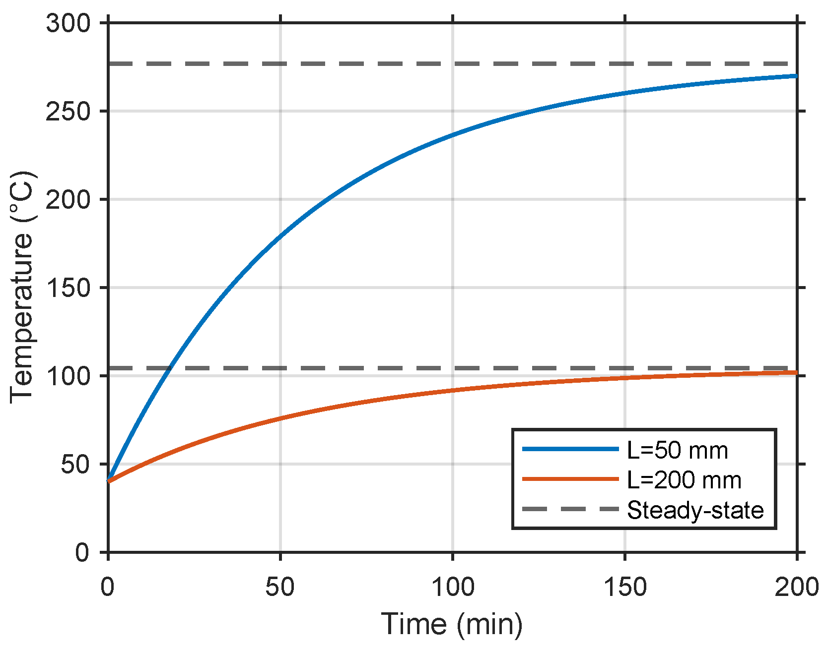
Steady-state temperature	$T_{ss}$	$276.8$ °C	$104.4$ °C

summarizes the main steady-state and dynamic results for both cases. Figure 6 depicts the thermal transient for the two geometries.

The results highlight the strong dependence of the steady-state temperature on the effective convective exchange area. Increasing the axial length significantly reduces the equivalent thermal resistance, while the total thermal capacitance increases proportionally with volume. As a consequence, the dominant time constant remains of the same order of magnitude (approximately one hour in both configurations), whereas the steady-state temperature decreases from about 277 °C for the 50 mm inductor to approximately 104 °C for the 200 mm configuration.

The short inductor clearly operates beyond typical insulation thermal limits (about 150 °C), confirming that, under the assumed loss and convection conditions, the convective surface-to-volume ratio is the dominant parameter governing the global thermal equilibrium.

A one-dimensional radial thermal model was implemented in order to account for the internal heat generation in both the ferrite core and the copper winding region. The geometry is assumed axisymmetric, with heat transfer occurring only in the radial direction. Convective heat exchange is applied exclusively at the external radius $r=R_2$, while symmetry is imposed at $r=0$. The initial condition for the transient simulations is the ambient temperature. For the steady-state solution, for each domain $i\in \{\mathrm{core},\mathrm{wind}\}$, the steady-state temperature distribution is given by Equation (12). The transient solution is expressed as Equation (14). In the 1D formulation, convection is applied only at the outer radius $r=R_2$, consistently with the assumption of purely radial heat transfer ($\partial /\partial z=0$). Axial heat spreading and end-face cooling are therefore not represented in this model.

The same geometrical configurations as in the previous subsection were analyzed: a short inductor ($L=50$ mm) and a long inductor ($L=200$ mm).

Table 7. Thermal 1D simulation results for the two inductor lengths.

Quantity	Symbol	$\mathit{L}=50$ mm	$\mathit{L}=200$ mm
Heat generation density in the core	${\dot{q}}_{core}$	$1.273\times {10}^4$ W/m3	$3.183\times {10}^3$ W/m3
Heat generation density in the winding	${\dot{q}}_{wind}$	$2.865\times {10}^6$ W/m3	$7.162\times {10}^5$ W/m3
Peak temperature	$T_{max}$	305.28 °C	106.32 °C
Surface temperature	$T\left(R_2\right)$	305.26 °C	106.31 °C

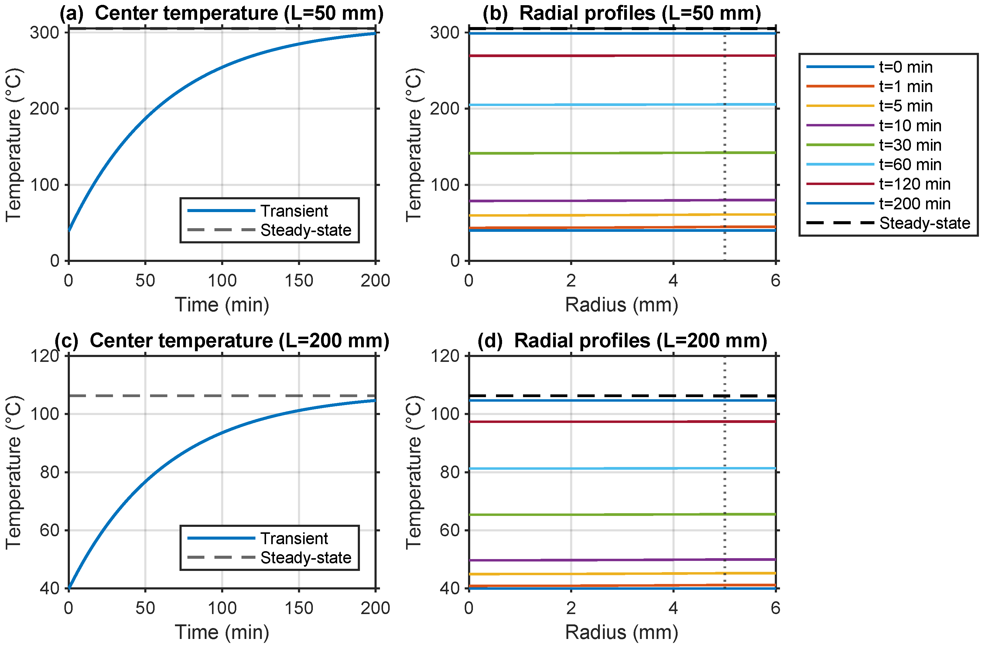
summarizes the steady-state peak temperature (at $r=0$), the external surface temperature. Figure 7 depicts the thermal transient for the two geometries at the center of the core.

Regarding the time constants, the transient solution in Equation (14) can be expressed as a sum of exponentially decaying modes, with modal time constants:

$${\tau }_n={\displaystyle \frac{1}{{\lambda }_n^2\alpha }}.$$

(44)

For the 1D model, only the first time constant of 3804 s (63.4 min) is considered as the higher modes decay within fractions of a second and are therefore negligible for thermal characterization purposes. The results confirm that radial temperature gradients remain very small in both geometries. This behavior is primarily due to the limited radial thickness of the winding region and the relatively high effective radial conductivity of the composite structure. As a consequence, the peak temperature and the external surface temperature differ by only a few hundredths of a degree.

Conversely, the axial length strongly influences the steady-state temperature through its impact on the convective exchange area. The short inductor ($L=50$ mm) reaches a steady-state temperature of approximately 305 °C, while the longer configuration stabilizes around 106 °C.

To capture both radial and axial heat spreading as well as end-face cooling effects, a 2D axisymmetric transient heat conduction model was implemented in the $(r,z)$ domain according to Equation (10). In this work, the steady-state and transient temperature fields were evaluated numerically on the 2D domain under the same loss partition adopted in the previous sections ($P_{core}=0.01P_{loss}$, $P_{wind}=0.99P_{loss}$).

Two geometrical configurations were analyzed: a short inductor ($L=50$ mm) and a long inductor ($L=200$ mm).

Table 8. 2D axisymmetric model results.

Quantity	$\mathit{L}=50\mathbf{mm}$	$\mathit{L}=200\mathbf{mm}$
Maximum temperature $T_{max}$	289.26 °C	107.82 °C
Mid-plane surface temperature $T(R_2,z=L/2)$	289.24 °C	107.81 °C

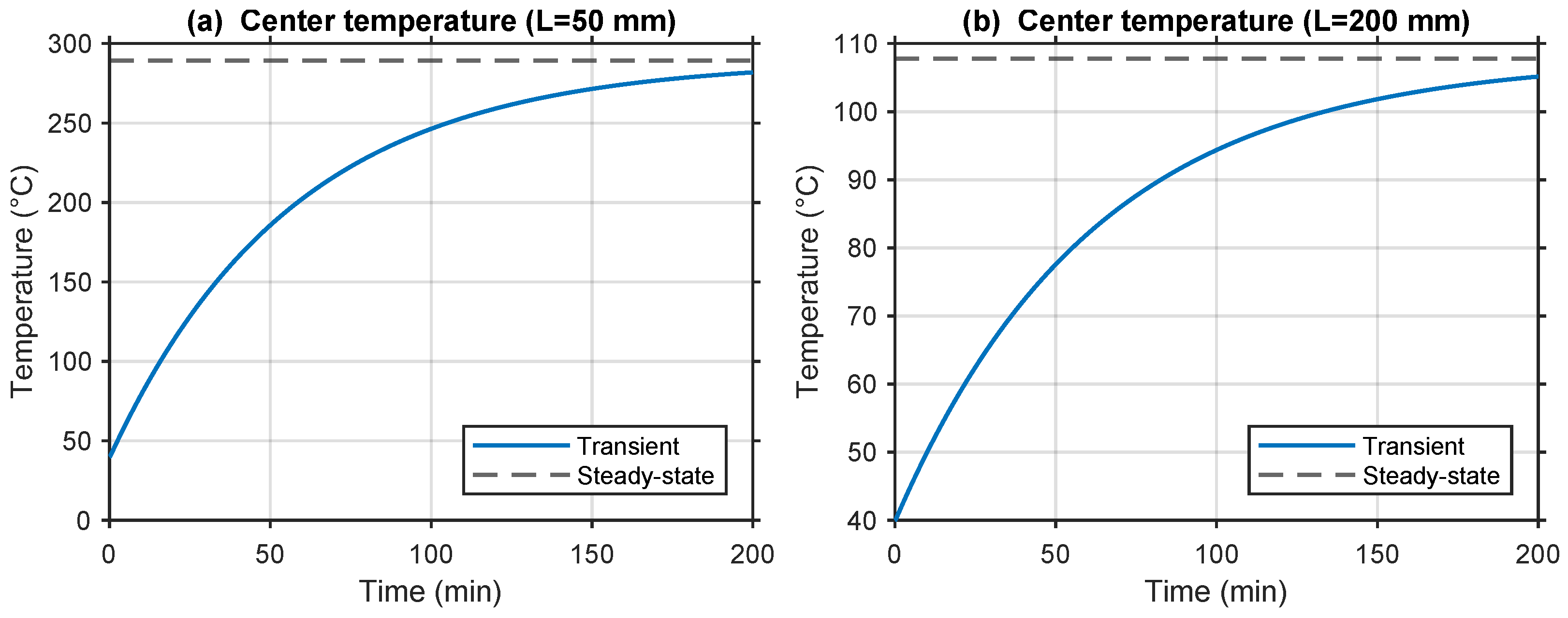
summarizes the main steady-state metrics (maximum temperature and mid-plane surface temperature) and Figure 8 depicts the transient temperatures at the core center location $(r=0,z=L/2)$ for the short and long inductors.

In the 2D formulation, the transient solution (Equation (10)) consists of double-indexed modes of the form

$$e^{-({\lambda }_m^2+{\mu }_n^2)\alpha t},$$

with corresponding modal time constants

$${\tau }_{m,n}={\displaystyle \frac{1}{({\lambda }_m^2+{\mu }_n^2)\alpha }}.$$

(45)

Table 9. 2D axisymmetric modal time constants (${\tau }_{m,n}>0.1$ s).

Mode $(\mathit{m},\mathit{n})$	$\mathit{L}=50$ mm	$\mathit{L}=200$ mm
(1,1)	3396 s ($56.6$ min)	3693 s ($61.6$ min)
(1,2)	$2.06$ s	$32.64$ s
(1,3)	$0.515$ s	$8.22$ s
(1,4)	$0.229$ s	$3.66$ s
(1,5)	$0.129$ s	$2.06$ s
(1,6)	–	$1.32$ s
(1,7)	–	$0.916$ s
(1,8)	–	$0.673$ s
(1,9)	–	$0.515$ s
(1,10)	–	$0.407$ s

reports the modal time constants truncated to ${\tau }_{m,n}>0.1$ s. The dominant dynamics is governed by the $(1,1)$ mode, while higher-order axial modes become relevant only in the longer configuration due to the reduced axial eigenvalues.

The 2D axisymmetric model confirms the trends already observed with the reduced-order formulations. The steady-state maximum temperature and the mid-plane surface temperature remain nearly coincident, indicating negligible radial gradients under uniform heat generation and symmetric boundary conditions.

Figure 8 reports the transient evolution of the temperature at the core center ($r=0,z=L/2$) for both geometrical configurations. The dynamic behavior exhibits a dominant first-order response, with a time constant consistent with the 0D and 1D predictions.

The short inductor ($L=50$ mm) reaches a steady-state temperature of approximately 289 °C, while the longer configuration stabilizes around 108 °C. The difference is primarily attributable to the increased lateral and end-face convective area in the longer geometry.

From a modal perspective, the transient solution can be expressed as a superposition of exponentially decaying modes (Equation (45)). However, only the $(1,1)$ mode significantly contributes to the minute-scale dynamics, while higher-order modes decay within seconds and do not influence the global thermal response.

5.4. Second Benchmark: Large-Radius Cylindrical Inductor

To further clarify when the 2D formulation becomes advantageous, an additional benchmark case was considered by increasing the overall radial size of the inductor while preserving the same thermal input assumptions adopted in the previous subsections. In particular, the inner radius of the core was set to $R_1=30$ mm and the external one, relative to the winding region, to $R_2=32$ mm. As in the previous case, two axial lengths were investigated, namely $L=50$ mm and $L=200$ mm.

The motivation for introducing this second family is that a larger radius-to-length ratio enhances the relative importance of axial heat spreading and end-face cooling. Therefore, although the winding thickness remains limited, the thermal field exhibits a more evident two-dimensional character, especially for the shorter configuration. This makes the larger-radius geometry particularly useful for highlighting the limitations of the 1D radial approximation and for clarifying under which geometric conditions the 2D model provides a non-negligible correction.

As a first observation, the 0D model still provides the reference prediction for the global average thermal inertia of the system. The validity of the lumped approach (Biot number lower than 0.1) was also verified with this geometry.

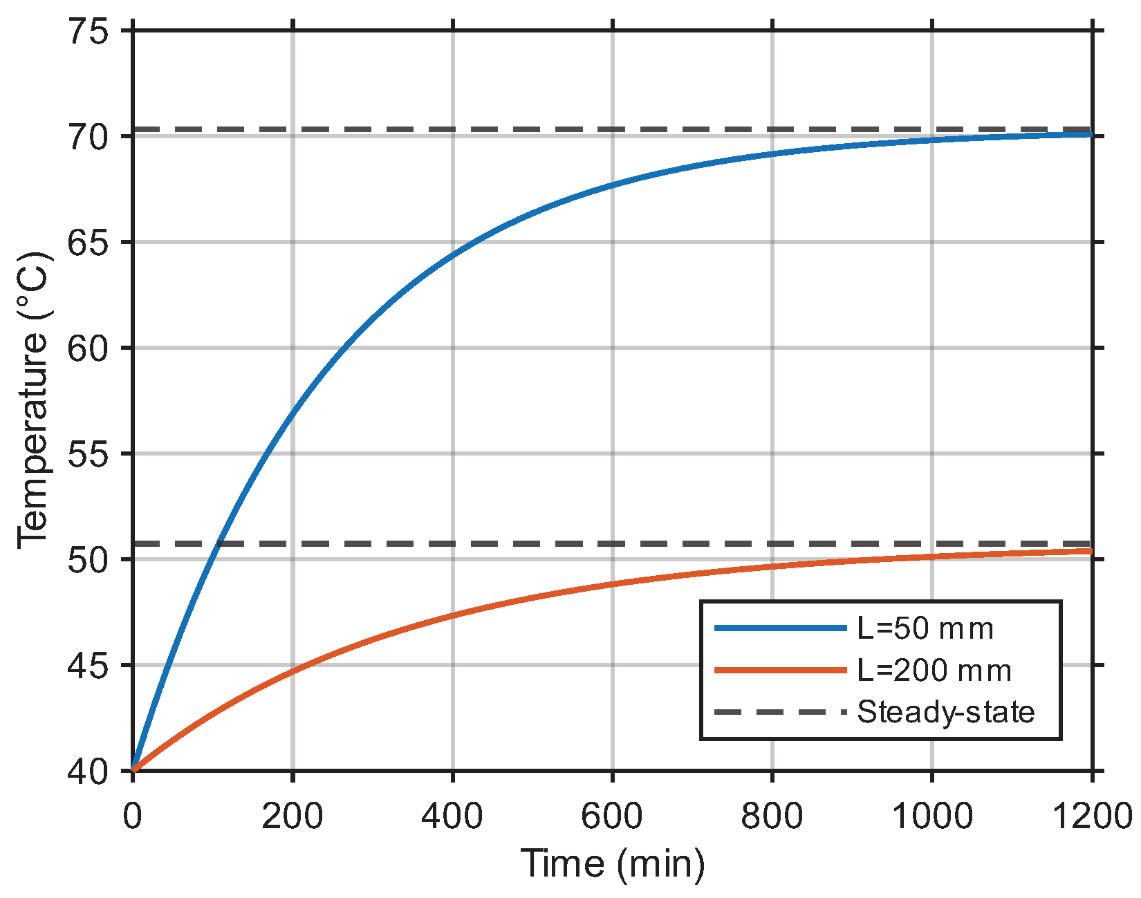
However, because the external exchange area and the internal heated volume are both modified by the larger diameter, the steady-state temperature levels and the equivalent thermal time constants differ from those obtained for the previous geometry. The resulting 0D transient responses for the two axial lengths are reported in Figure 9.

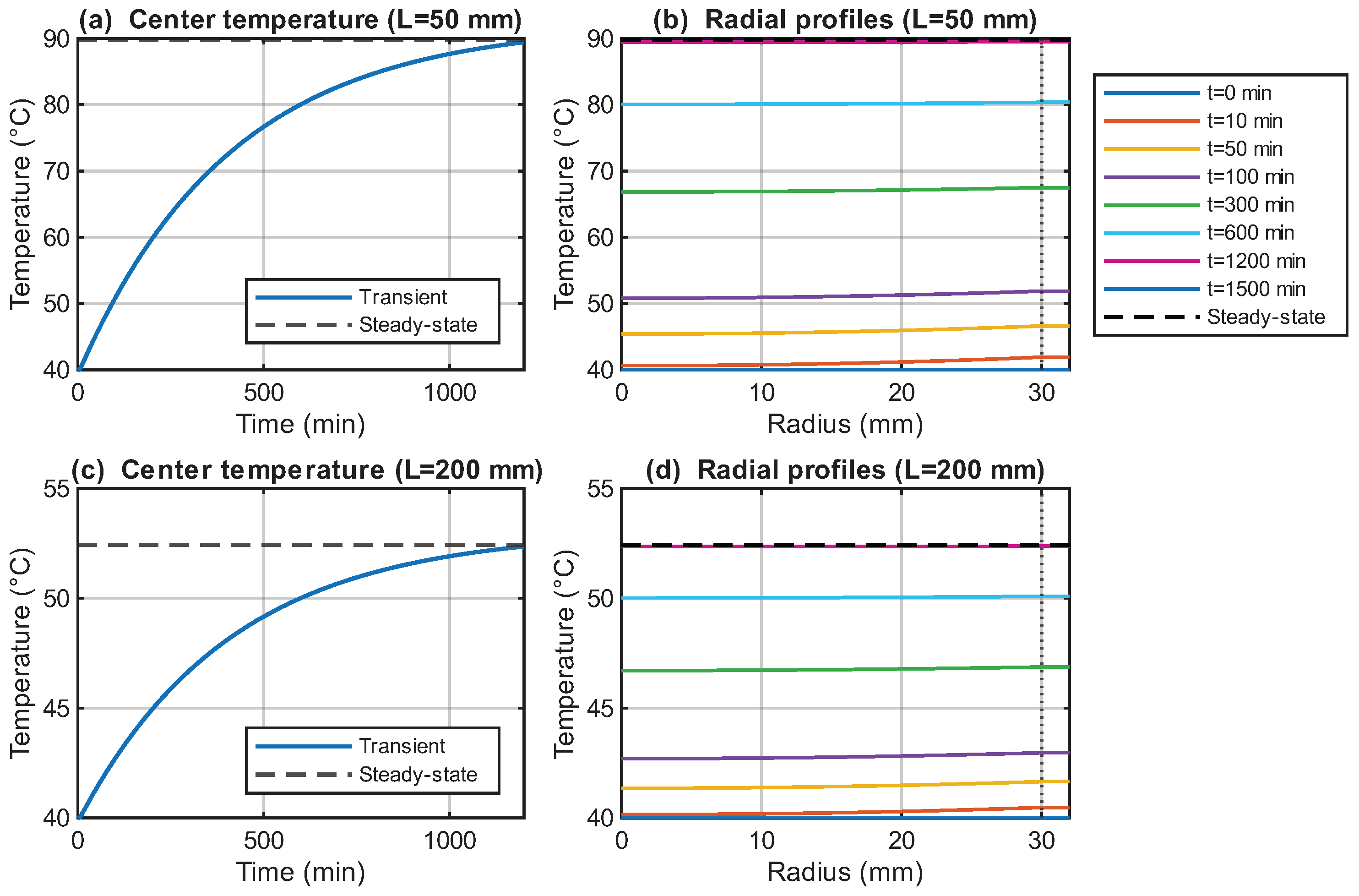
The 1D radial model was then applied to the same larger-radius geometries. Since the radial thickness of the winding region remains limited, purely radial gradients remain moderate also in this case. Nevertheless, the 1D model does not account for heat exchange through the two end faces and therefore cannot represent the increased role of axial heat removal when the geometry is changed. The corresponding 1D transient responses and representative radial profiles are reported in Figure 10. A relevant difference emerges in the short configuration ($L=50$ mm), for which the 1D model predicts a significantly higher steady-state temperature than the 2D formulation, with a deviation of about 27%. By contrast, for the long configuration ($L=200$ mm), the 1D steady-state temperature remains much closer to the reduced-order predictions, confirming that axial effects become less important as the inductor becomes more slender.

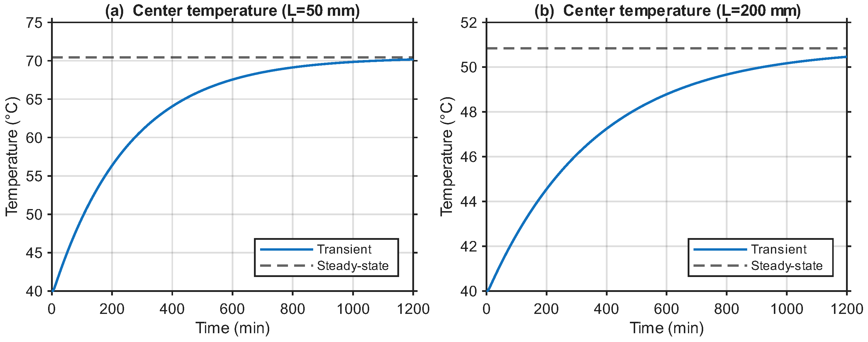
Finally, the 2D axisymmetric model was used to capture the full radial–axial temperature field. In this second benchmark family, the 2D formulation provides a more visible correction with respect to the 1D model, especially for the short inductor, because the contribution of the end surfaces to the total heat exchange becomes more relevant and the axial temperature distribution is no longer negligible. 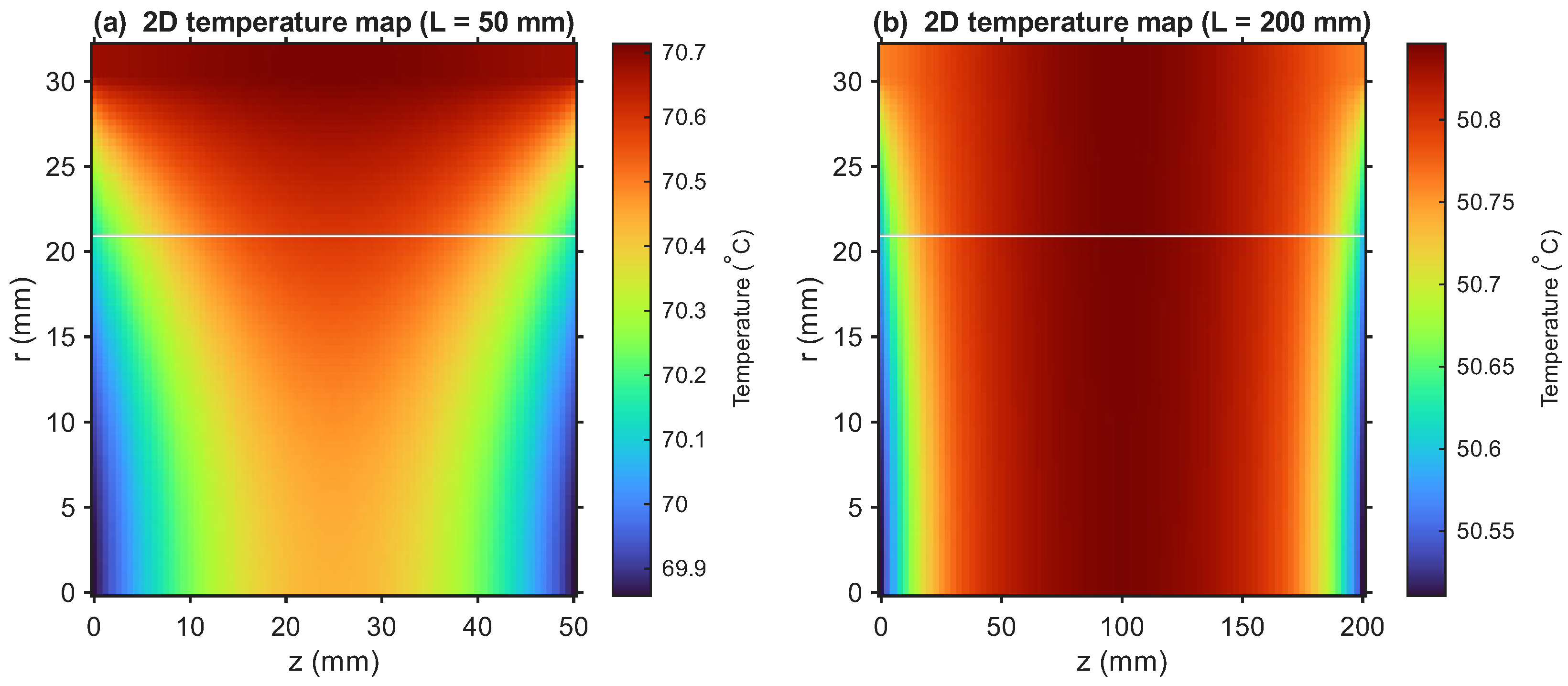The transient evolution at the geometric center is reported in Figure 11, while the corresponding steady-state temperature maps are shown in Figure 12.

From a physical standpoint, this second benchmark family strengthens the interpretation already emerging from the small-radius geometry. More specifically, the longer configuration remains reasonably well-described by reduced-order formulations, whereas the shorter configuration exhibits a more pronounced discrepancy between 1D and 2D predictions. This confirms that the benefit of the 2D model is not only related to the presence of localized losses or asymmetric boundary conditions, but can already become relevant when the component geometry increases the relative importance of axial heat spreading and end-face cooling.

The 2D results also show that the radial temperature variation remains very small in all four cases, with nearly uniform temperature from the cylinder axis to the external radius. Therefore, the discrepancy between the 1D and 2D predictions is not associated with stronger radial gradients, but with the axial component of heat transfer. In particular, the 2D formulation captures axial heat spreading and convective heat removal through the end faces, whereas the 1D model neglects both effects. This becomes especially important for the short large-radius inductor, for which the deviation between the 1D and 2D hot-spot predictions reaches 26.93%, while it decreases to 3.13% for the long configuration. Hence, the benefit of the 2D model in this benchmark is mainly related to axial thermal effects rather than to radial non-uniformity.

5.5. Comparative Analysis of 0D, 1D and 2D Predictions

The three modeling approaches are compared in terms of hot-spot temperature, spatially averaged temperature, dominant transient response, and axial temperature non-uniformity. The comparison is carried out over the two benchmark families introduced above, namely the small-radius cylindrical inductor and the large-radius cylindrical inductor, each evaluated for two axial lengths.

A first important result concerns the distinction between global and local thermal predictions. In all the considered cases, the 0D model provides the average temperature evolution and captures the dominant thermal inertia of the inductor with minimal computational effort. The dominant time constant remains on the order of one hour, consistently with the first mode extracted from the 2D formulation. This confirms that the global thermal dynamics is governed by a single slow mode, whereas higher-order spatial modes decay within seconds or fractions of a second.

For the first benchmark family, namely the small-radius cylindrical inductor, the agreement among the three modeling levels remains generally good. In particular, for the long configuration ($L=200$ mm), the 1D and 2D models provide very similar steady-state temperatures, indicating that axial gradients are weak and that the thermal behavior is predominantly radial. The deviation between the 1D and 2D hot-spot predictions is only 1.39% in this case. For the short configuration ($L=50$ mm), the 2D model predicts a lower steady-state hot-spot temperature than the 1D model because it explicitly captures end-face cooling and axial heat spreading. In this case, the deviation between the 1D and 2D hot-spot predictions increases to 5.54%. Therefore, for the small-radius benchmark family, reduced-order formulations still provide a reasonably accurate description of the global thermal response, while the 2D formulation mainly refines the local temperature distribution.

A more pronounced difference emerges in the second benchmark family, characterized by the larger radius. In this case, the shorter configuration exhibits a much stronger two-dimensional thermal character. The increased radial size enhances the relative importance of the end surfaces in the global heat exchange, so that the 1D radial approximation becomes less accurate. For the short large-radius inductor, the discrepancy between the 1D and 2D hot-spot predictions reaches 26.93%, clearly showing that neglecting axial heat spreading and end-face cooling may lead to a substantial overestimation of the local peak temperature. By contrast, for the long large-radius inductor, the deviation decreases to 3.13%, indicating that axial non-uniformity weakens as the component becomes more slender.

These results show that the practical need for a 2D formulation is not determined only by the presence of localized losses or asymmetric cooling, but also by the component aspect ratio. The axial gradient indicator $\Delta T_z\left(t\right)$ remains limited for the long configurations of both benchmark families, whereas it becomes much more relevant in the short large-radius case, consistently with the larger discrepancy observed between the 1D and 2D models.

The comparison further confirms that reduced-order formulations remain effective when the design objective is the estimation of global thermal metrics, such as average temperature evolution and dominant time constant. However, this agreement in global quantities does not imply equivalent accuracy in local hot-spot prediction. The present results clearly show that local discrepancies may become significant even when the global thermal inertia is still well-described by a lumped model.

From an engineering standpoint, the benchmark suggests the following model-selection guideline. The 0D model is appropriate for fast estimation of average temperature rise and dominant thermal inertia. The 1D model is suitable when radial resolution is required and axial gradients remain weak, which is generally the case for sufficiently slender cylindrical inductors. The 2D model becomes necessary when end-face effects, aspect-ratio effects, asymmetric boundary conditions, or non-uniform loss distributions must be resolved with adequate fidelity.

It is also worth noting that the experimental validation presented in Section 5.1 supports the capability of the model to reproduce the measured outer thermal response and the dominant transient behavior. Therefore, the benchmark discussion developed here should be interpreted as an extension of that validated framework toward the comparison of different thermal model orders, rather than as a purely abstract analytical exercise.

It should be emphasized that the present comparison is performed under uniform loss distribution and symmetric convection. Different conclusions may arise under strongly localized heat sources, mounting-induced asymmetry, or coupled electro–thermal conditions. Even under these simplified assumptions, however, the second benchmark family demonstrates that geometry alone can make the 2D formulation significantly more informative than reduced-order alternatives.

For engineering use, the main applicability range of the three modeling levels can be summarized as reported in

Table 10. Recommended application scope of the considered thermal modeling levels.

Model	Recommended Use	Main Strength	Main Limitation
0D lumped	Preliminary design, fast parametric scans, average temperature estimation, dominant thermal time constant evaluation	Very low computational cost; directly captures global thermal inertia and average temperature rise	Cannot resolve internal gradients, hot-spots, axial effects, or local cooling conditions
1D radial	Cylindrical inductors with mainly radial heat flow, uniform losses, and weak axial gradients	Includes internal radial conduction with limited complexity; suitable when the component is slender and boundary conditions are nearly uniform along the axis	Neglects axial heat spreading and end-face cooling; may overestimate hot-spot temperature when axial effects become relevant
2D radial–axial	Short or thick cylindrical inductors, components with significant end-face cooling, asymmetric axial boundary conditions, localized cooling, or non-uniform loss distribution	Captures both radial and axial heat transfer, providing the most reliable hot-spot prediction under axisymmetric assumptions	Higher mathematical and computational complexity; requires additional assumptions on spatial loss distribution and boundary conditions

.

6. Conclusions

This work presented a benchmark-oriented analytical comparison of thermal modeling approaches for cylindrical inductive components used in power electronic systems. Starting from the general heat conduction equation in cylindrical coordinates, three modeling levels were formulated and discussed: lumped (0D), radial (1D), and radial–axial (2D) transient models.

The comparative application to two benchmark families of two-layer cylindrical inductors highlighted the influence of both axial length and radial size on steady-state temperature, transient evolution, and spatial gradients. Despite the increased mathematical complexity of the 2D formulation, the results demonstrate that, under uniform internal heat generation and symmetric convective boundary conditions, the global thermal behavior is still dominated by a single slow mode. The associated time constant remains on the order of one hour for the considered geometries, while higher spatial modes decay within fractions of a second and do not significantly affect minute-scale dynamics.

For the small-radius benchmark family, the 0D model provides a good prediction of the average thermal behavior, while the 1D radial model yields results close to the 2D formulation when axial gradients remain weak. In this case, the benefit of the 2D model is mainly associated with a more accurate description of end-face cooling and axial heat spreading in the short configuration. More specifically, the deviation between the 1D and 2D hot-spot predictions is 5.54% for the short configuration and 1.39% for the long one.

The second benchmark family, characterized by a larger radius, further clarifies the practical relevance of the 2D formulation. In particular, the short large-radius inductor exhibits a much more pronounced discrepancy between 1D and 2D predictions, with the hot-spot deviation reaching 26.93%, while the corresponding deviation decreases to 3.13% for the long configuration. This shows that geometry alone can significantly enhance the role of axial heat spreading even under uniform losses and symmetric convection. The result demonstrates that the need for 2D modeling is strongly geometry-dependent and cannot be assessed solely on the basis of winding thickness or radial conductivity.

From an engineering standpoint, the comparison also enables a practical model-selection criterion. The 0D formulation is sufficient when only the average temperature rise and the dominant thermal time constant are required. The 1D model is appropriate for cylindrically symmetric inductors when radial conduction is of interest and axial gradients remain weak. The 2D formulation should instead be preferred when the component geometry enhances axial heat spreading, when convective exchange through the end faces is not negligible, or when boundary conditions and loss distributions are spatially non-uniform. For clarity, the recommended application scope of each modeling level is summarized in Table 10.

The experimental validation performed on the small-radius, long inductor further supports the proposed framework. In particular, the 1D and 2D models both reproduce the measured external thermal transient with high accuracy, with RRMSE values of 0.0138 and 0.0106, respectively, while the 2D model yields the smallest quasi-steady-state error (0.133 °C). By contrast, the 0D model correctly captures the dominant heating dynamics but underestimates the measured external temperature because of its lumped nature. These results confirm that, for slender cylindrical inductors and uniform operating conditions, reduced-order formulations already provide an accurate prediction of the external thermal response.

The experimental comparison should be interpreted accordingly: the present setup validates the model against externally measured thermal quantities, whereas internal hot-spot predictions remain inaccessible to direct measurement and therefore retain a model-based character. Future work may address this aspect through embedded sensing, inverse thermal identification, or coupled electro–thermal experiments specifically designed to infer the internal temperature field.

Overall, the proposed analytical framework establishes quantitative criteria for selecting the appropriate thermal modeling level based on the required accuracy and computational complexity, thereby supporting reliability-oriented design and electro–thermal co-analysis of inductive components in high power density converters. The presented framework can also serve as a benchmark reference for validating reduced-order numerical or finite-element models.