Analysis and Modeling of Physical Evolution Mechanism for High-Resistance to Low-Resistance Grounding Faults in 10 kV Cable Joints

Abstract

Currently, the lack of analysis and applicable circuit models for the evolution of cable joint faults is responsible for explosions or fire accidents in the distribution network system. In this paper, the modeling of high-resistance to low-resistance grounding faults for 10 kV cable joints is investigated. Firstly, the physical evolution from high-resistance to low-resistance grounding faults in 10 kV cable joints is analyzed. Secondly, the common discharge characteristics under different evolution stages are extracted by simulation experiments and fault-recording data. Thirdly, an interface breakdown circuit model and a radial breakdown circuit model are established to quantitatively describe the high-resistance to low-resistance grounding faults of cable joints. Fourthly, the corresponding arc resistance models are proposed, and the controlled parameter values of the models under different evolution stages are given. Finally, the fault identification control model is implemented for relay protection. This paper provides theoretical and modeling support for the fault identification of 10 kV cable joints, filling the knowledge gap of this critical fault type in relay protection.

1. Introduction

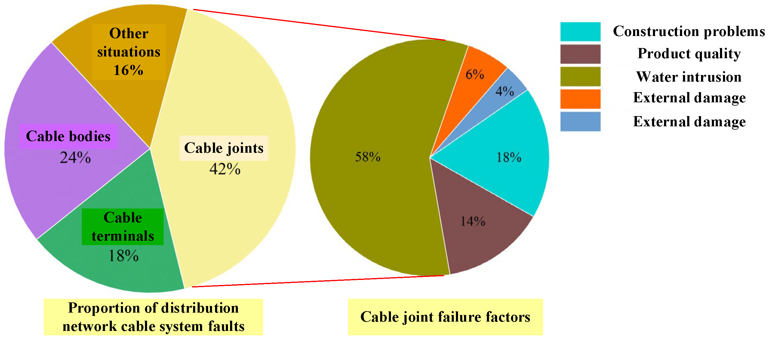
Generally, 10–35 kV medium voltage cables are widely used in the distribution network system. With the increasing number of branches and growing complexity [1], the failure rate of the system has been increasing year by year in China. Due to the complex interface characteristics of medium voltage cable joints [2,3], they become a weak point in distribution network systems. Figure 1 exhibits a statistical diagram of the types of faults in the distribution network cable system provided by a power supply bureau in southern China. In hundreds of cable joint failure cases, it is found that the interface breakdown [4] at the crosslinked polyethylene (XLPE)–silicon rubber (SiR) insulation interface is the general origin of the fault. Subsequently, the radial breakdown of the XLPE and the SiR insulations is triggered by the interface breakdown, which may cause serious explosions and fire accidents in extreme cases [5,6,7]. Additionally, the cable joint fault on one feeder often triggers the failure of defective equipment of other feeders on the same busbar as a result of intense voltage fluctuations [8]. The main reason for this consequence is that the existing relay protective system in the distribution network has a risk of failure in identifying and recovering the high-resistance grounding fault of cable joints, which exacerbates internal defects in cable joints gradually.

Currently, power supply stability is preferentially guaranteed in the distribution network. It is mainly reflected in the large setting current, long setting time, and reclosing operation after trip protection of the protective relaying system. This strategy is suitable for judging the low-resistance grounding faults on the overhead lines and cable lines [9,10]. However, the strategy can barely identify or prevent cable joint faults. The brief reasons are as follows. (1) At the early or intermediate failure stage, there is a risk of relay protective system failure in the evolution of the cable joint fault. (2) At the late failure stage, the indiscriminate reclosing operation of the protective relaying system activated by low-resistance grounding faults may result in the grounding failure of cable joints and cause serious accidents. Therefore, with the development of relay protection in new power systems, identifying the cable joint faults and eliminating their potential threat in advance are of great significance for improving the safety and stability of distribution network systems.

Given that high-resistance and low-resistance grounding faults are generally accompanied by nonlinear arcs, arc models based on the theory of thermal equilibrium have been successively proposed, such as the Mayr arc model, the Cassie arc model, and their improved arc models [11,12,13]. The above models can effectively present various typical air arcs and explain the periodic zero-crossing phenomenon of high-resistance grounding faults. However, the changes in arc characteristics during the whole physical evolution of high-resistance to low-resistance grounding faults in cable joints have not been well reported in the existing literature. In fact, there is a distinct difference between the organic insulation of cable joints and the gas insulation [14]. The pyrolysis of organic insulation caused by discharges not only affects the discharges themselves but also results in different discharge paths inside the cable joints. In addition, an interactive coupling relationship exists between fault current and insulation states during the evolution from high-resistance to low-resistance grounding faults, which has not been considered in existing models. Thus, it is necessary to analyze the physical evolution of the cable joint faults and establish corresponding circuit models with arc models for the enhancement of sensitivity in identifying cable joint faults.

This paper concentrates on two perspectives. Firstly, the physical evolution of the cable joint faults is explored to construct a corresponding circuit model based on the physical structure of cable joints. Secondly, combined with the experimental and fault-recording data, equivalent discharge circuit models with arc models in the axial and radial directions are established, and the electrical parameters are provided.

The evolution process of high-resistance grounding to low-resistance grounding fault of cable joints is discussed first in the paper; the high-resistance grounding fault is classified as XLPE-SiR insulation interface breakdown, and the low-resistance grounding fault is classified as radial breakdown. Secondly, models are given to describe the insulation interface breakdown and radial breakdown, and the range of parameters in the model is given. Finally, the control model of high-resistance grounding to low-resistance grounding fault of cable joints is given.

2. Analysis of the Physical Evolution from High-Resistance to Low-Resistance Grounding Faults in 10 kV Cable Joints

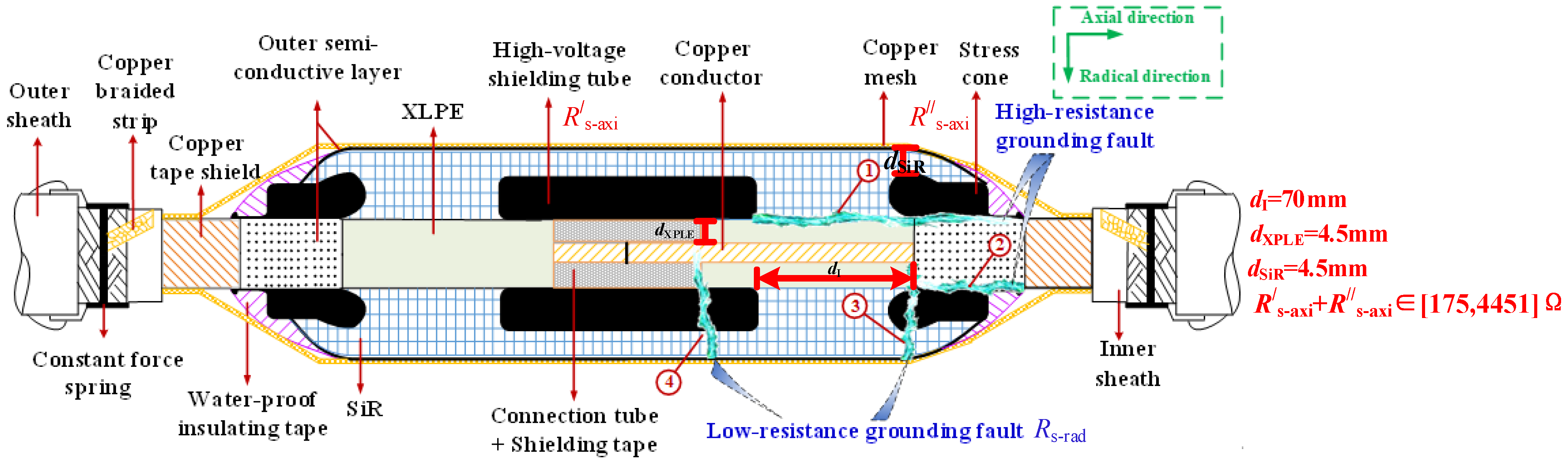
According to the statistical analysis of hundreds of failure cases, it is determined that the faults of the cable joint are induced by the arcs with different discharge paths, as shown in Figure 2, where the number of ①②③ represent the fault path in the cable joints; the colors of the figure represent different parts of the cable joint and fault path. Most of the faulty cable joints originate from the interface breakdown at the XLPE-SiR insulation interface, as shown in the discharge path ① in Figure 2. This is a high-resistance grounding fault, which is ascribed to aging, poor manufacture, water intrusion, silicone grease swelling [15], etc. Subsequently, the radial breakdown of XLPE insulation at the end of the stress cone is generally triggered by interface breakdown [6]. The discharge current is first connected to the copper tape shield through the outer semiconducting layer, as shown in the discharge path ② in Figure 2. Meanwhile, the stress cone lies in high potential, followed by the breakdown of the remaining SiR insulation. Due to the existence of radial resistance of the stress cone, the current generated in the discharge path ③ is limited, which can be first regarded as a high-resistance grounding fault. As the stress cone carbonizes, a breakdown hole is generated, and stable arcs are formed in the breakdown path ③. This is a low-resistance grounding fault, resulting in the activation of the 1st trip protection. In addition, the impact of the switching surge caused by several reclosing operations is injected into the system, which may destroy the copper mesh of the cable joint and lead to grounding failure. This is responsible for the deactivation of zero-sequence protection and the subsequent explosion or fire accident. Additionally, the radial breakdown along the breakdown path ④ occasionally occurs within the cable joint. This situation is similar to that along the breakdown path ③, which will not be discussed in detail in the following text.

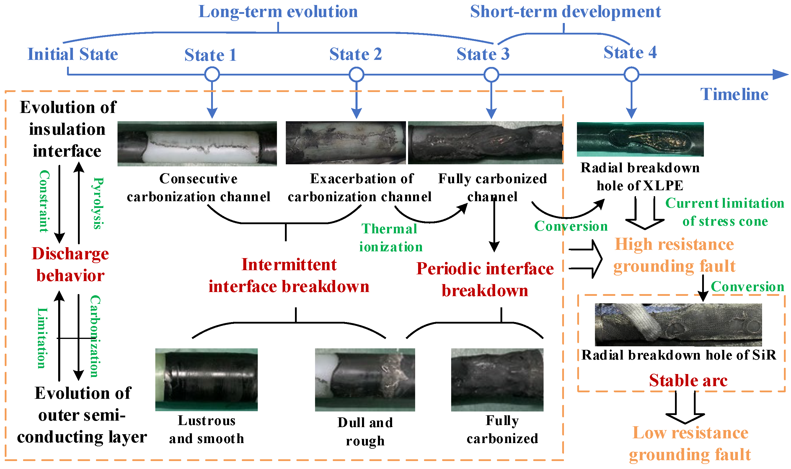
Based on the analysis of the cable joint faults mentioned above, a physical evolution diagram and the basis for subsequent modeling of discharge behaviors in faulty cable joints is exhibited in Figure 3, where the color red represents the discharge mode; the color orange represents the fault state; the color black represents the insulation state; the color blue represents the timeline of fault evolution; the color green represents the connection relationship. In the process of long-term evolution, a consecutive carbonization channel at the XLPE-SiR insulation interface is formed as a result of the intermittent interface breakdown. The initial interface breakdown voltage shows a decreasing trend as the carbonization channel continues to deepen and widen. Meanwhile, with the increase in the discharge repetition rate and discharge intensity, the resistance of the outer semi-conductive layer increases exponentially at first, which plays a vital role in limiting currents. When the outer semi-conductive layer carbonizes to a certain extent, the resistance declines sharply and the periodic interface breakdown is generated. In the process of short-term development, the breakdown of XLPE insulation at the end of the stress cone is regarded as the starting point. Transiently, the radial breakdown of the remaining SiR insulation occurs. The radial breakdown current is first constrained by the resistance of the stress cone. When the stress cone burns out a hole, a stable arc is formed.

From the perspective of the time scale, based on preliminary research and laboratory experiments, it has been investigated that the Initial State generally takes several years to reach State 1. This process is mainly influenced by the rates of silicone grease swelling and insulation interface water ingress. Further, the evolution from State 1 to State 3 can generally be transformed within a few hours under sufficient moisture conditions. Therefore, the high-resistance grounding fault caused by insulation interface discharges is a long-term evolutionary process. Conversely, for the low-resistance grounding fault caused by radial breakdown of insulations, it is determined that the conversion from State 3 to State 4 occurs within several seconds based on the actual fault-recording data. Thus, the low-resistance grounding fault caused by the radial breakdown of insulations is a short-term development.

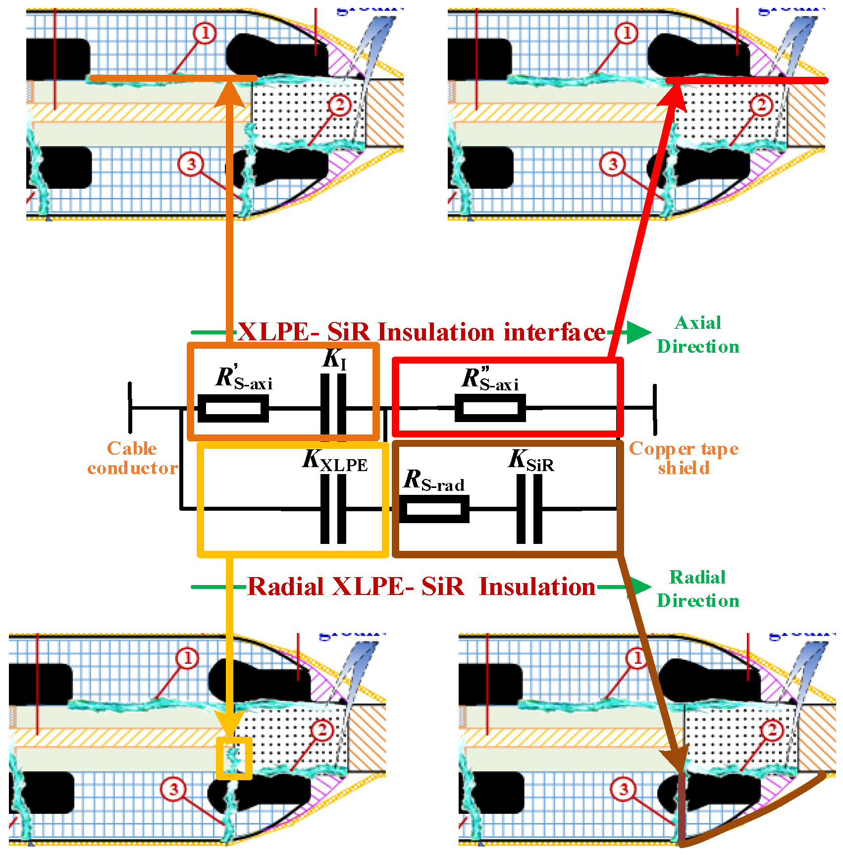
To explain the above phenomenon quantitatively and analyze the influence of physical changes in the cable joints on the discharge behavior, a circuit model based on the physical structure of the cable joint is established, as shown in Figure 4, where the numbers represent the fault path in the cable joint; the arrows represent the circuit modules and its physical correspondence in the cable joint; the colors represent different circuit modules. The physical correspondence of the circuit modules in Figure 4 are listed in

Table 1. Circuit modules and their physical correspondence in the cable joint.

Circuit Module	Physical Correspondence in the Cable Joint
Branch: $R_{\mathrm{S}-\mathrm{a}\mathrm{x}\mathrm{i}}^{\prime },$ KI	Resistance of the XLPE-SiR insulation interface breakdown tracking; dielectric strength of XLPE-SiR insulation interface
Branch: $R_{\mathrm{S}-\mathrm{a}\mathrm{x}\mathrm{i}}^{″}$	Resistance of the stress cone
Branch: KXLPE	Dielectric strength of radial XLPE insulation
Branch: RS-axi, KSiR	Equivalent resistance of axial semi-conductive layer; dielectric strength of radial SiR insulation

. The definition and calculation of each electrical parameter in the model are provided as follows.

(1) Dielectric strength of XLPE-SiR insulation interface K_I

$$K_{\mathrm{I}}={\displaystyle \frac{u_{\mathrm{b}}^{\prime }}{d_{\mathrm{I}}}}$$

(1)

where $u_{\mathrm{b}}^{\prime }$ is the interface breakdown voltage, V; d_I is the minimum discharge distance of the insulation interface, mm. For typical 10 kV cable joints, d_I = 70.0 mm. The value of K_I is determined by the state of the insulation interface, which is jointly affected by the factors of water intrusion, silicone grease swelling, pyrolysis of the insulations, etc.

(2) Dielectric strength of radial XLPE insulation K_XLPE

$$K_{\mathrm{XLPE}}={\displaystyle \frac{u_{\mathrm{b}}^{″}}{d_{\mathrm{XLPE}}}}$$

(2)

where $u_{\mathrm{b}}^{″}$ is the radial XLPE insulation breakdown voltage, V; d_XLPE is the thickness of the radial XLPE insulation, mm. The value of K_XLPE is influenced by the carbonization degree of the XLPE-SiR insulation interface. For typical 10 kV cable joints, d_XLPE = 4.5 mm.

(3) Dielectric strength of radial SiR insulation K_SiR

$$K_{\mathrm{SiR}}={\displaystyle \frac{u_{\mathrm{b}}^{‴}}{d_{\mathrm{SiR}}}}$$

(3)

where $u_b^{‴}$ is the radial SiR insulation breakdown voltage, V; d_SiR is the remaining thickness of SiR insulation, mm. For typical 10 kV cable joints, d_SiR = 4.5 mm.

It is noted that the parameters of K_I, K_XLPE, and K_SiR can only be obtained through experimental or fault-recording data, characterizing the zero-crossing time of the arc currents. It is reflected that under the condition of constant discharge distance, the smaller the dielectric strength, the smaller the breakdown voltage, and the shorter the zero-crossing time of the arc current.

(4) Equivalent resistance of axial semi-conductive layer R_S-axi

$$R_{\mathrm{S}-\mathrm{axi}}=R_{\mathrm{S}-\mathrm{axi}}^{\prime }+R_{\mathrm{S}-\mathrm{axi}}^{″}$$

(4)

$$R_{\mathrm{S}-\mathrm{axi}}^{\prime }={\rho }_{\mathrm{S}}(T){\displaystyle \frac{l_{\mathrm{S}-\mathrm{axi}}^{\prime }}{\mathsf{\pi }(r_{\mathrm{o}1}^2-r_{\mathrm{i}1}^2)}}$$

(5)

$$R_{\mathrm{S}-\mathrm{axi}}^{″}={\rho }_{\mathrm{S}}(T){\displaystyle \frac{l_{\mathrm{S}-\mathrm{axi}}^{″}}{\mathsf{\pi }(r_{\mathrm{o}2}^2-r_{\mathrm{i}2}^2)}}$$

(6)

where $R_{\mathrm{S}-\mathrm{a}\mathrm{x}\mathrm{i}}^{\prime }$ is the equivalent resistance of the high-voltage shielding tube along the axial direction, Ω; $R_{\mathrm{S}-\mathrm{a}\mathrm{x}\mathrm{i}}^{″}$ is the equivalent resistance of the outer semi-conductive layer along the axial direction, Ω; $l_{\mathrm{S}-\mathrm{a}\mathrm{x}\mathrm{i}}^{\prime }$ is the distance from the end of the high-voltage shielding tube to the connection tube, mm;$l_{\mathrm{S}-\mathrm{a}\mathrm{x}\mathrm{i}}^{″}$ is the distance from the outer semi-conductive layer to the copper tape shield, mm; $r_{\mathrm{o}1}$ and $r_{\mathrm{i}1}$ are the outer diameter and inner diameter of the semi-conductive layer on the cable body, mm;$r_{\mathrm{o}2}$ and $r_{\mathrm{i}2}$ are the outer diameter and inner diameter of the high-voltage shielding tube, mm; ${\rho }_{\mathrm{S}}\left(T\right)$ is the resistivity of semi-conductive layer materials, Ω∙mm. ${\rho }_{\mathrm{S}}\left(T\right)$ possesses a positive temperature coefficient (PTC) characteristic, which increases exponentially as the temperature T increases. The range of this parameter is 200~4000 Ω∙mm within the range of 25~90 °C [16]. It is calculated that the range of R_S-axi of 10 kV cable joints with 400 mm² cross-section and above is [175, 4451] Ω.

(5) Equivalent radial resistance of stress cone R_S-rad

$$R_{\mathrm{S}-\mathrm{rad}}={\displaystyle \frac{{\rho }_{\mathrm{S}}\left(T\right)}{2\mathsf{\pi }{l}_{\mathrm{S}-\mathrm{rad}}}}\ln {\displaystyle \frac{r_{\mathrm{o}1}}{r_{\mathrm{i}1}}}$$

(7)

where $l_{\mathrm{S}-\mathrm{r}\mathrm{a}\mathrm{d}}$ is the axial length of the stress cone, mm. It is noted that the stress cone structure is simplified here as a cylindrical ring for calculation. Based on the structure of 10 kV cable joints, it is calculated that the range of R_S-rad is [20, 400] Ω.

3. Establishment of Interface Breakdown Circuit Model Based on Simulation Experiments

3.1. Experiment

3.1.1. Sample Preparation

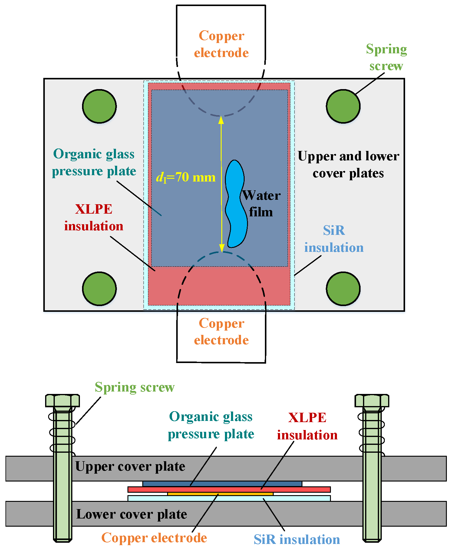
Several XLPE and SiR samples with a size of 10 × 5 cm were prepared for the interface breakdown experiment. Firstly, the distance between two electrodes at the XLPE-SiR interface was regulated to 7 cm, which is consistent with that of actual cable joints. Secondly, 0.1% ammonium chloride (NH₄Cl) solution was added to one end of the samples to form a water film, which simulates one-way water ingress in actual cable joints. Thirdly, the samples were set based on the combination shown in Figure 5. To simulate the actual interface pressure of cable joints, 0.25 MPa of pressure was applied to the samples through the springs. Fourthly, samples with varying degrees of damage were produced by means of the experiments in Section 3.1.2. This setting simulates the different stages of interface breakdown evolution of cable joints.

3.1.2. Experimental Method

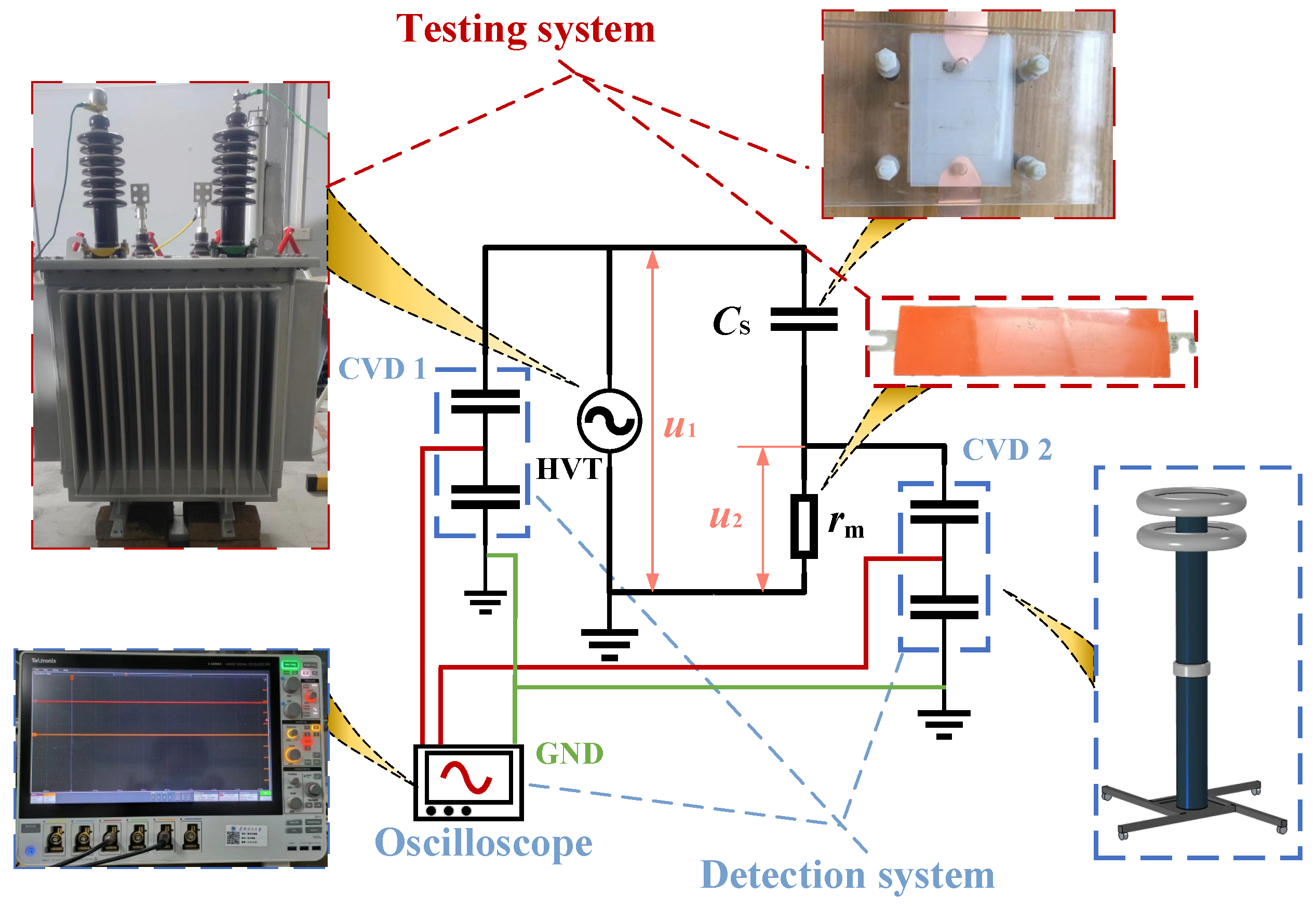
The schematic diagram of the test is shown in Figure 6. Where HVT is the high-voltage transformer with a capacity of 110 kVA (22 kV, 5 A), r_m is the non-inductive measured resistance (360, 540, and 4400 Ω), which is equivalent to R_S-axi of cable joints. C_s is the selected sample where one electrode was connected to the high voltage, and the other electrode was connected to r_m; CVD1 and CVD2 are the capacitive voltage dividers, which are applied to measure the voltages of HVT (u₁) and r_m (u₂). The sampling frequency of the oscilloscope is set to 6.25 GS/s (the sampling time, T_s = 0.16 ns) with 350 MHz bandwidth. The input voltage u₁ was set at 5.8 kV (the phase voltage of 10 kV) for each experiment to obtain the waveforms of u₁ and u₂. Finally, the interface breakdown voltage u_I(t) and the interface breakdown current i_b can be calculated by Equations (8) and (9).

$$u_{\mathrm{I}}\left(t\right)=u_1\left(t\right)-u_2\left(t\right)$$

(8)

$$i_{\mathrm{b}}(t)={\displaystyle \frac{u_2\left(t\right)}{r_{\mathrm{m}}}}$$

(9)

3.2. Experiment Results

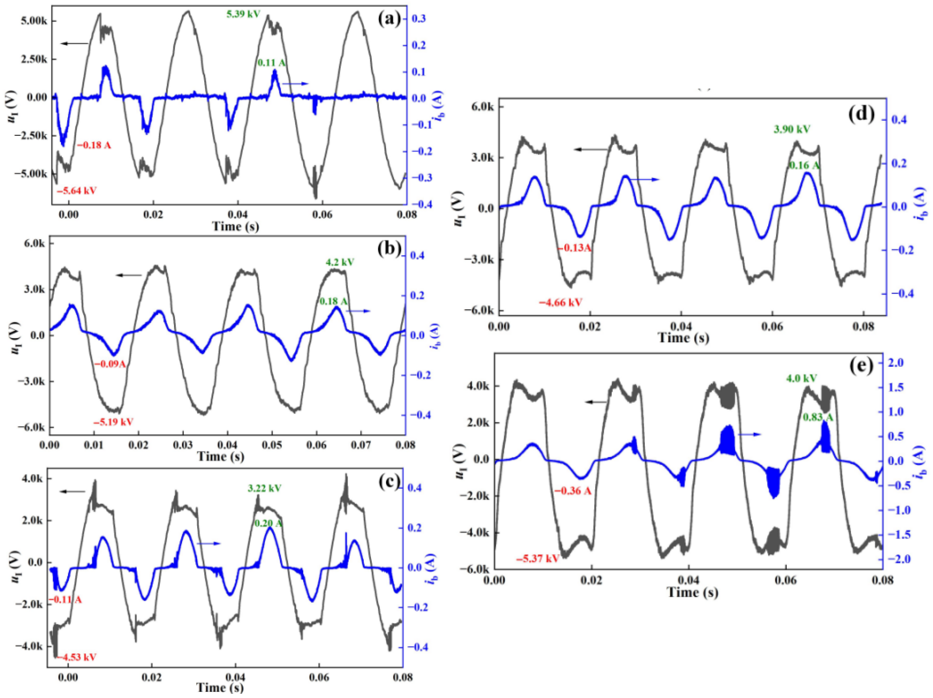
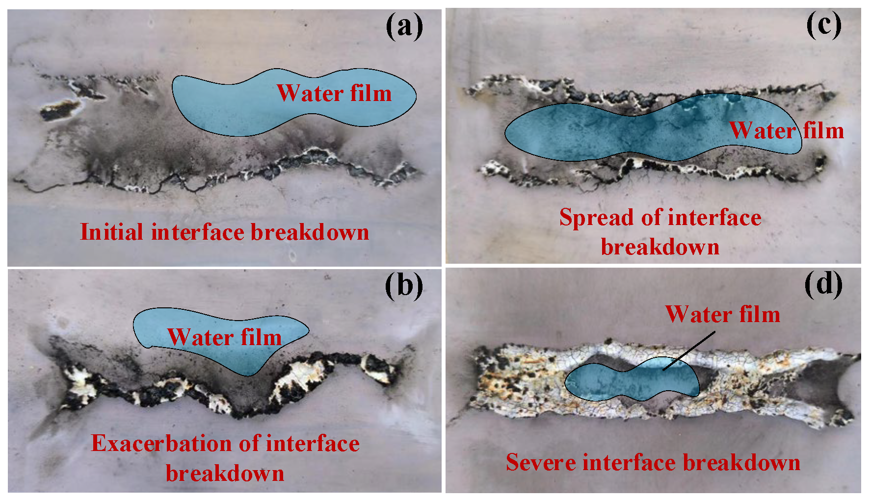
Figure 7 exhibits the evolution of the interface breakdown waveforms of u_i and i_b in the experiment’s tests. Firstly, a 360 Ω testing resistance (r_m in Figure 6) was connected to the testing circuit, which is equivalent to R_S-axi at room temperature. When the applied voltage reaches 5.3~5.6 kV, intermittent interface breakdown occurs at the insulation interface as displayed in Figure 7a. As a consecutive carbonization channel generates and the water spreads, the discharge repetition rate gradually increases, resulting in the periodic interface breakdown as shown in Figure 7b. It is found that the interface breakdown voltage declines to 4.2~5.2 kV, and the zero-crossing time becomes shortened. Even though the present external circuit resistance (360 Ω) is low, the equivalent interface breakdown resistance of the insulation interface is high enough to constrain the arc current, reflecting the high-resistance characteristics. After observing the samples in Figure 8a, it was discovered that the discharge path is along the edge of the water film due to the intense electric field at the wet–dry interface. As the number of interface breakdowns increases, the carbonization channel becomes deeper and wider, as shown in Figure 8b, which in turn augments the interface breakdown intensity.

Secondly, the samples with a consecutive carbonization channel and water were prepared for the test. Considering the exponential increase in R_S-axi caused by the thermal effect of periodic interface breakdown current in actual cable joints, the testing resistance of 540 Ω and 4400 Ω was connected to the testing circuit, respectively. The waveforms of u_i and i_b are exhibited in Figure 7c,d. It is discovered that the waveforms of i_b are similar to those of the intermediate stage, and the equivalent interface breakdown resistances become lower. Since the initial carbonization channel accelerates the permeation of the water, the spread of the interface breakdown occurs as shown in Figure 8c. The formation of a new carbonization channel strengthens discharge intensity. At this stage, the external circuit resistance (mainly R_S-axi) becomes the main current-limiting component, which still conforms to the feature of high-resistance grounding faults.

Thirdly, under the long-term influence of periodic interface breakdown, the axial semi-conductive layer of the cable joint is inclined to be carbonized, and R_S-axi decreases sharply eventually. The samples with severe carbonization channels and water were prepared for the test with 360 Ω. At this stage, it is found that there are violent discharges with strong light generated at the XLPE-SiR interface, corresponding to the arcs with numerous superimposed pulse currents in Figure 7e. Due to the decline of the current-limiting effect, fierce arc currents can be generated, and the discharge paths become heater and heater. This process ionizes more free molecules, and thermoelectric ionization is triggered. Further, the equivalent interface breakdown resistance sharply declines, which in turn aggravates the next discharge. Eventually, large-scale discharge damage appears on the insulation interface, as shown in Figure 8d.

4. Interface Breakdown Circuit Modeling and Its Arc Resistance Model

4.1. Interface Breakdown Circuit Model

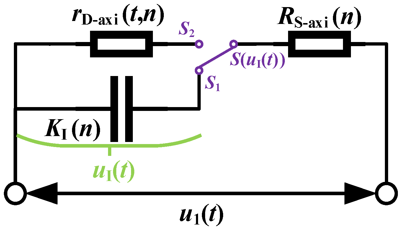
Combined with discharge path ① in Figure 2 and the above experimental results, an interface breakdown circuit model of cable joints is established, as shown in Figure 9. Where r_D-axi is the equivalent interface breakdown resistance, Ω, S(u_I(t)) is the switching function, characterizing the zero-crossing time of the interface breakdown currents. It is pointed out that r_D-axi is a time-varying nonlinear arc resistance, which is changed with time (t) and affected by the evolutionary state (n) of the material. Likewise, the value of K_I and R_S-axi is related to the evolutionary state (n) of the material. These two parameters jointly determine the switching direction of S(u_I(t)). When the applied voltage u_I(t) exceeds the interface breakdown voltage, S(u_I(t)) switches from S₁ to S₂. These arcs tend to be extinguished as a result of the drop in u_I(t) and the current limitation of R_S-axi. Subsequently, S(u_I(t)) returns to S₁. Thus, the function of S(u_I(t)) is given by Equation (10).

$$S(u_{\mathrm{I}}(t))=\left\{\begin{array}{c}{S}_2,u_{\mathrm{I}}\left(t\right)\ge u_{\mathrm{I}}\left(t_0\right)=K_{\mathrm{I}}\left(n\right)\cdot d_{\mathrm{I}}\\ S_{\mathrm{1}},u_{\mathrm{I}}\left(t\right)<u_{\mathrm{I}}(t_0+T_{\mathrm{a}})\end{array}\right.$$

(10)

where t₀ is the initial time of the interface breakdown, ms; T_a is the interface breakdown arcing duration with abnormal voltage, ms. On the basis of the experimental results in Figure 8, t₀ and T_a can be obtained. Furthermore, the measured u_I(t₀) (i.e., $u_b^{\prime }$) can be substituted into Equation (1) to obtain K_I.

4.2. Interface Breakdown Arc Model

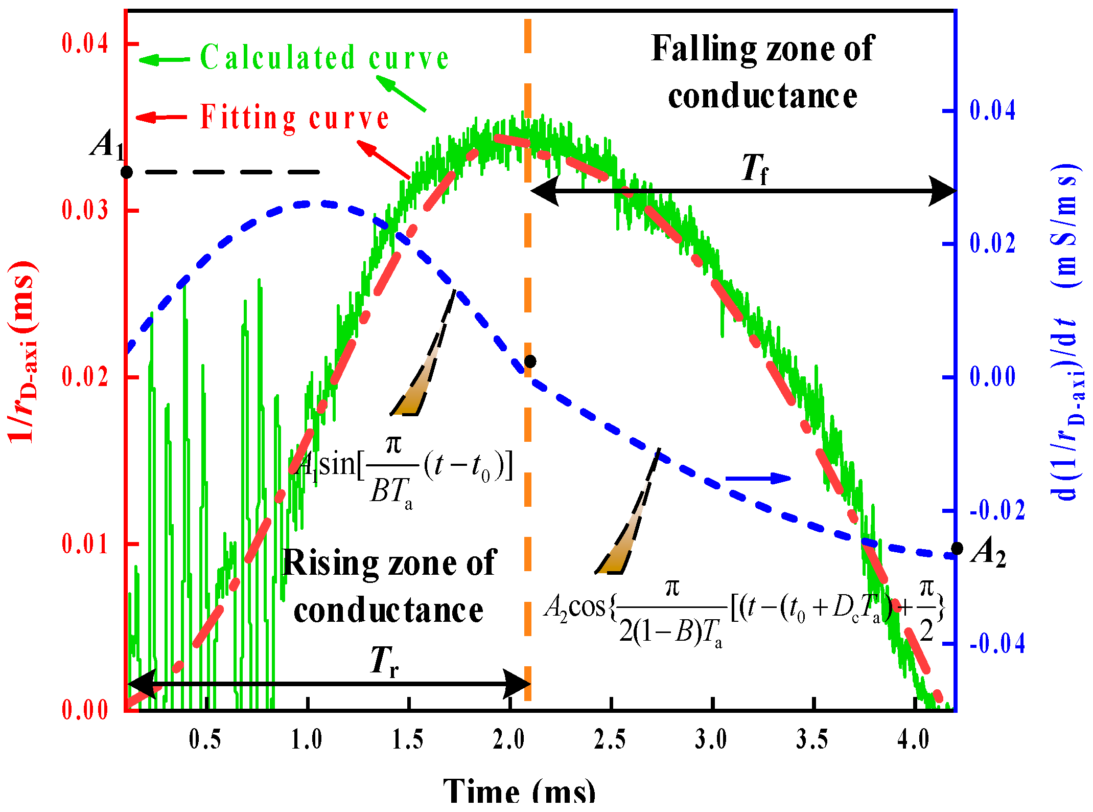
For the determination of r_D-axi in the interface breakdown circuit model of cable joints, an interface breakdown arc resistance model is proposed. The constructing method is displayed in Figure 10.

Firstly, based on the experimental results in Figure 7, the parameter of 1/r_D-axi during arcing can be calculated. It is observed that there are two zones of rising zone and falling zone of conductance, separated by the peak value of 1/r_D-axi. Thus, the following correlations are obtained.

$$T_{\mathrm{a}}=T_{\mathrm{r}}+T_{\mathrm{f}}$$

(11)

$$B={\displaystyle \frac{T_{\mathrm{r}}}{T_{\mathrm{a}}}}$$

(12)

where T_r is the interface breakdown arcing duration in the rising zone of conductance, ms; T_f is the interface breakdown arcing duration in the falling zone of conductance, ms; B is the ratio of T_r to T_a.

Secondly, it is observed that the calculated curve of 1/r_D-axi can barely be fitted by quadratic functions. To avoid excessive fitting coefficients and insufficient physical representation when using higher-order functions for fitting, a segmented trigonometric function is applied to approximate the main features of the time-variable nonlinear arc resistance [17]. In the rising zone of 1/r_D-axi, the curve of 1/r_D-axi is approximately fitted as a cosine function with an angular frequency of π/(BT_a) and a phase range of [π, 2π]. In the falling zone of 1/r_D-axi, the curve of 1/r_D-axi is approximately fitted as a cosine function with an angular frequency of π/(2(1 − B)T_a) and a phase range of [π/2, π]. Therefore, the interface breakdown arc resistance model is expressed as follows:

$${\displaystyle \frac{\mathrm{d}(1/r_{\mathrm{D}-\mathrm{axi}})}{\mathrm{d}t}}=\left\{\begin{array}{c}{A}_1\sin [{\displaystyle \frac{\mathsf{\pi }}{B{T}_{\mathrm{a}}}}(t-t_0)],t_0\le t<t_0+B{T}_{\mathrm{a}}\\ A_2\cos \{{\displaystyle \frac{\mathsf{\pi }}{2(1-B)T_{\mathrm{a}}}}[(t-(t_0+B{T}_{\mathrm{a}})+{\displaystyle \frac{\mathsf{\pi }}{2}}\},t_0+B{T}_{\mathrm{a}}\le t<T_{\mathrm{a}}+t_0\end{array}\right.$$

(13)

where A₁ is the amplitude of the changing rate in the rising region of conductance, mS/ms; A₂ is the amplitude of the changing rate in the falling region of conductance, mS/ms.

Thirdly, combined with the experimental results and Equation (13), the ranges of the controlled parameters of the interface breakdown circuit model under different stages of interface breakdown evolution of cable joints are listed in

Table 2. Control parameters of interface breakdown circuit model.

Parameter	Control Function	Value Range
		Initial Stage (360 Ω)	Intermediate Stage (360 Ω)	Transition Stage 1 (540 Ω)	Transition Stage 2 (4.4 kΩ)	Last Stage (360 Ω)
KI (kV/cm)	Zero-crossing time	0.76~0.80	0.60–0.74	0.46~0.64	0.56~0.67	0.57–0.77
t0 (ms)	Initial arcing time	1.2~4.0	1.2~3.2	0.8~2.3	1.3~1.7	1.6~2.0
Ta (ms)	Arcing duration	3.3~3.5	4.9~6.9	4.4~6.5	6.5~7.5	6.8~7.9
A1 × 10−2/(mS/ms)	Rising amplitude	0.94~1.32	0.77~1.34	1.73~3.74	0.14~0.26	3.66~5.48
A2 × 10−2/(mS/ms)	Falling amplitude	1.69~3.43	1.78~3.67	3.94~7.87	0.32~0.63	3.04~27.80
B (%)	Rising zone width	0.33~0.566	0.63~0.64	0.48~0.50	0.60~0.61	0.60~0.61

.

5. Establishment of Radial Breakdown Circuit Model Based on Fault-Recording Data

5.1. Analysis of the Fault-Recording Data of an Authentic Case

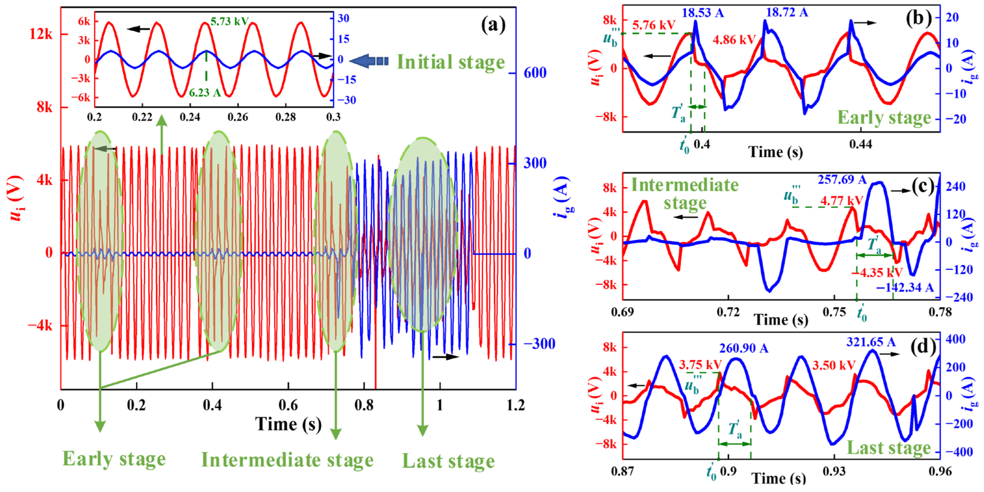
Based on the fault-recording data of the literature [6], the evolution of high-resistance to low-resistance grounding faults of a cable joint has been well-recorded. Considering the topological characteristics of distribution lines, the correlation between the input bus voltage u_i and the grounding current i_g of the faulty distribution line detected in the substation is shown in Figure 11, where the color green and arrows represent different stage of radial breakdown faults in cable joints. In Figure 11a, it is found that a weak sinusoidal current consistently exists in the whole process. It is deduced that a breakdown hole of the XLPE insulation has been formed, and the arc currents have passed through the discharge path ② to the ground in Figure 2. Due to the existence of the outer semi-conductive layer, the arc currents are limited to 7 A without causing an obvious voltage drop. This stage is regarded as an initial stage of the radial breakdown evolution. Meanwhile, the stress cone of the cable joint withstands a high potential, and the discharge path ③ in Figure 2, caused by the intermittent radial breakdown, is generated in a short time. The arc currents are constrained by the radial resistance of the stress cone. With the continuous carbonization of the stress cone and the expansion of the breakdown hole, u_i and i_g are changed correspondingly. The early stage, intermediate stage, and last stage are proposed to describe the radial breakdown evolution of cable joints. The corresponding discharge signals are shown in Figure 11b–d. In Figure 11b, it is indicated that the arc currents are below 19 A, and the radial breakdown arcing times are about 5 ms. In the early stage, the arc currents are greatly limited by the resistance of the stress cone. In the intermediate stage shown in Figure 11c, the maximum amplitude of the arc current reaches 257.7 A, and the radial breakdown arcing times extend over 6 ms, indicating that the stress cone becomes severely carbonized. In the last stage shown in Figure 11d, the maximum amplitude of the arc current reaches 321.7 A, and the radial breakdown arcing times extend to about 10 ms. In this case, it is denoted that a radial breakdown hole is formed in the discharge pathway ③, resulting in the generation of low-resistance arcs. The currents of these arcs reach 321.7 A and basically cover the full cycle of i_g.

5.2. Radial Breakdown Circuit Modeling and Its Arc Resistance Model

5.2.1. Radial Breakdown Circuit Model

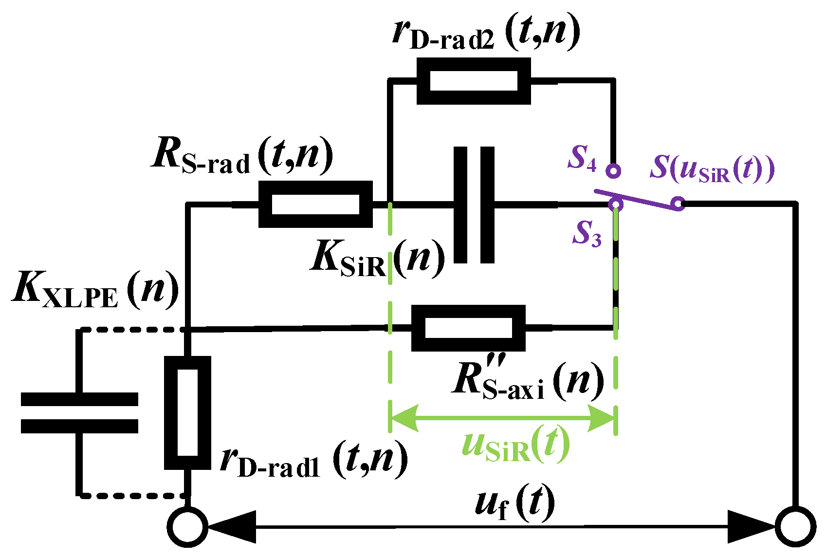
Combined with the discharge path ② and ③ in Figure 2 and the above fault-recording data, a radial breakdown circuit model of cable joints is established as shown in Figure 12. u_f is the fault point voltage, V; r_D-rad1 is the equivalent radial breakdown resistance of XLPE, Ω; r_D-rad2 is the equivalent radial breakdown resistance of SiR, Ω; S(u_SiR(t)) is the switching function, characterizing the extinguishing time of the radial breakdown currents. In this case, it is deduced that a breakdown hole in the XLPE insulation has been formed, and stable periodic arcs are generated. For simplicity, the influence of K_XLPE is ignored. Moreover, it is pointed out that r_D-rad1 and r_D-rad2 are time-varying nonlinear arc resistances, which are changed with time (t) and affected by the evolutionary state (n) of the material. Similarly, the value of K_SiR, K_XLPE, and R_S-rad is related to the evolutionary state (n) of the material. When the applied voltage u_SiR(t) exceeds the radial breakdown voltage of SiR, S(u_SiR(t)) switches from S₃ to S₄. These arcs tend to be extinguished as a result of the drop in u_SiR(t) and the current limitation of R_S-rad. Subsequently, S(u_SiR (t)) returns to S₃. Thus, the function of S(u_SiR(t)) is given by (14).

$$S(u_{\mathrm{SiR}}(t))=\left\{\begin{array}{c}{S}_4,u_{\mathrm{SiR}}\left(t\right)\ge u_{\mathrm{SiR}}\left(t_0^{\prime }\right)=K_{\mathrm{SiR}}\left(n\right)\cdot d_{\mathrm{SiR}}\\ S_3,u_{\mathrm{SiR}}\left(t\right)<u_{\mathrm{SiR}}(t_0^{\prime }+T_{\mathrm{a}}^{\prime })\end{array}\right.$$

(14)

where $t_0^{\prime }$ is the time of the initial radial breakdown voltage of the remaining SiR insulation, ms; $T_{\mathrm{a}}^{\prime }$ is the radial breakdown arcing time with abnormal voltage, ms. The controlled parameters of radial breakdown circuit model in Figure 12 is listed in the

Table 3. Controlled parameters of radial breakdown circuit model.

Parameter	Controlled Function	Value Range
		Early Stage	Intermediate Stage	Last Stage
KSiR (kV/cm)	Extinguishing time	10.8~12.8	9.7~10.6	7.8~8.3
$t_0^{\prime }$ (ms)	Initial arcing time	6.7~4.2	3.6~0.7	1.3~0.0
$T_{\mathrm{a}}^{\prime }$ (ms)	Arcing duration	3.3~5.8	6.4~9.3	8.7~10.0

.

5.2.2. Radial Breakdown Arc Model

For the determination of r_D-rad1 and r_D-rad2 in the radial breakdown circuit model of cable joints, a radial breakdown arc resistance model is proposed in this section. According to the fault-recording data in Figure 11, it is observed that radial breakdown arc waves are diverse under different stages of radial breakdown evolution. In this paper, Kizilcay’s arc model [18,19] is adopted to approximate the radial breakdown arc resistance r_D-rad. The constructing function expression is illustrated as follows.

$${\displaystyle \frac{\mathrm{d}(1/r_{\mathrm{D}-\mathrm{rad}})}{\mathrm{d}t}}={\displaystyle \frac{1}{\tau }}({\displaystyle \frac{\left|i_{\mathrm{g}}\right|}{u_0+r_0\left|i_{\mathrm{g}}\right|}}-1/r_{\mathrm{D}-\mathrm{rad}})$$

(15)

$$1/r_{\mathrm{D}-\mathrm{rad}}={\displaystyle \frac{\left|i_{\mathrm{g}}\right|}{u_0+r_0\left|i_{\mathrm{g}}\right|}}\cdot {\displaystyle \frac{1}{1+s\tau }}={\displaystyle \frac{G_{\mathrm{S}}}{1+s\tau }}$$

(16)

where u₀ is the characteristic arc voltage, V; r₀ is the characteristic arc resistance, Ω; τ is the arc time constant, s; G_S is the transfer conductance, S. It is noted that Equation (16) is the transfer function of Equation (15) by using the Laplace transform, which is applied to the following PSCAD modeling.

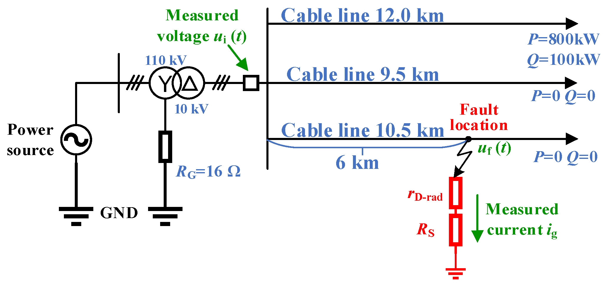
To validate the practicability of Kizilcay’s arc model for the different evolution stages of radial breakdown, the fault line topology with the arc model is established by PSCAD software (version5.0) in Figure 13, where R_S is the equivalent semi-conductive resistance; the arrows represent the measured physical quantity; the colors represent the name of different circuit component in the circuit; the symbol represent different circuit component, which is a variable parameter for different evolution stages. Further, the simulated results are shown in Figure 14, where the arrows represent the resistance for semi-conductor of different semi-conductor competent in the cable joint; the green line is the zero baseline of current and voltage. The corresponding controlled parameters [19,20] of the arc model are listed in

Table 4. Controlled parameters of radial breakdown arc model.

Parameter	Value Range
	Initial Stage	Early Stage	Intermediate Stage	Last Stage
τ (ms)	0.3	0.3	0.1	0.3
u0 (V)	750	750	2000	1200
r0 (Ω)	0.01	0.01	0.01	0.01
RS (Ω)	800	280	5	0

.

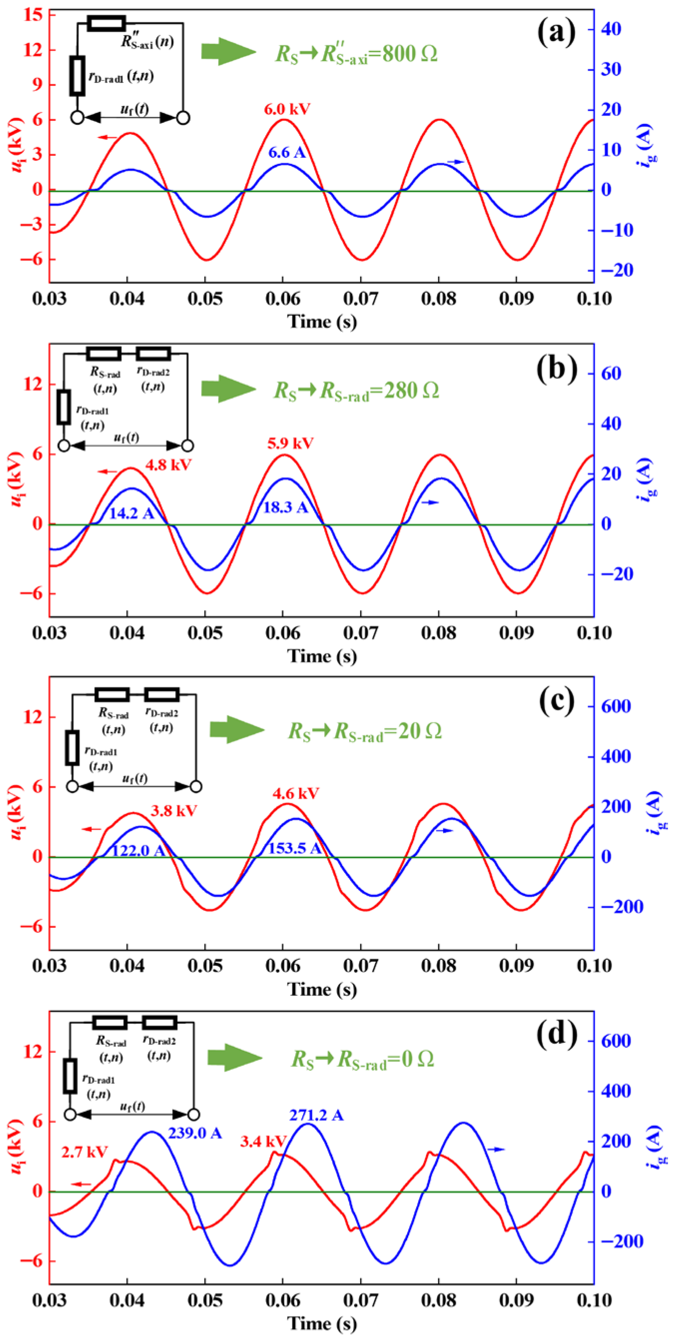
In the initial stage of radial breakdown evolution, the simulated result is shown in Figure 14a. Combined with the result shown in Figure 11a, it is found that Kizilcay’s arc model can approximate the waveforms of u_i and i_g well. In this stage, the controlled parameter of r_D-rad represents r_D-rad1 and R_S represents $R_{\mathrm{S}-\mathrm{a}\mathrm{x}\mathrm{i}}^{″}$. The simulated result shows that this is a high-resistance grounding fault of cable joints with R_S of 800 Ω in the circuit (Breakdown path ② in Figure 2).

In the subsequent three stages shown in Figure 14b–d, the arc current flows through r_D-rad1, R_S-rad, and r_D-rad2 (Breakdown path ③ in Figure 2). Thus, the controlled parameter of r_D-rad represents r_D-rad1 + r_D-rad2 and R_S represents R_S-rad. Compared with the three stages, it is observed that R_S decreases monotonically as the radial breakdown continues. When the radial breakdown hole is generated, R_S equals zero and a low-resistance grounding fault occurs.

Even though the simulated amplitudes of u_i and i_g are close to the fault-recording data, the waveforms in Figure 14b,c can barely be consistent with that of the fault-recording data. Thus, it is admitted that, for the transient transition of the early stage and the intermediate stage, the arc characteristics cannot be completely reproduced through Kizilcay’s arc model.

6. Implementation of Fault Identification Control Model of Cable Joints

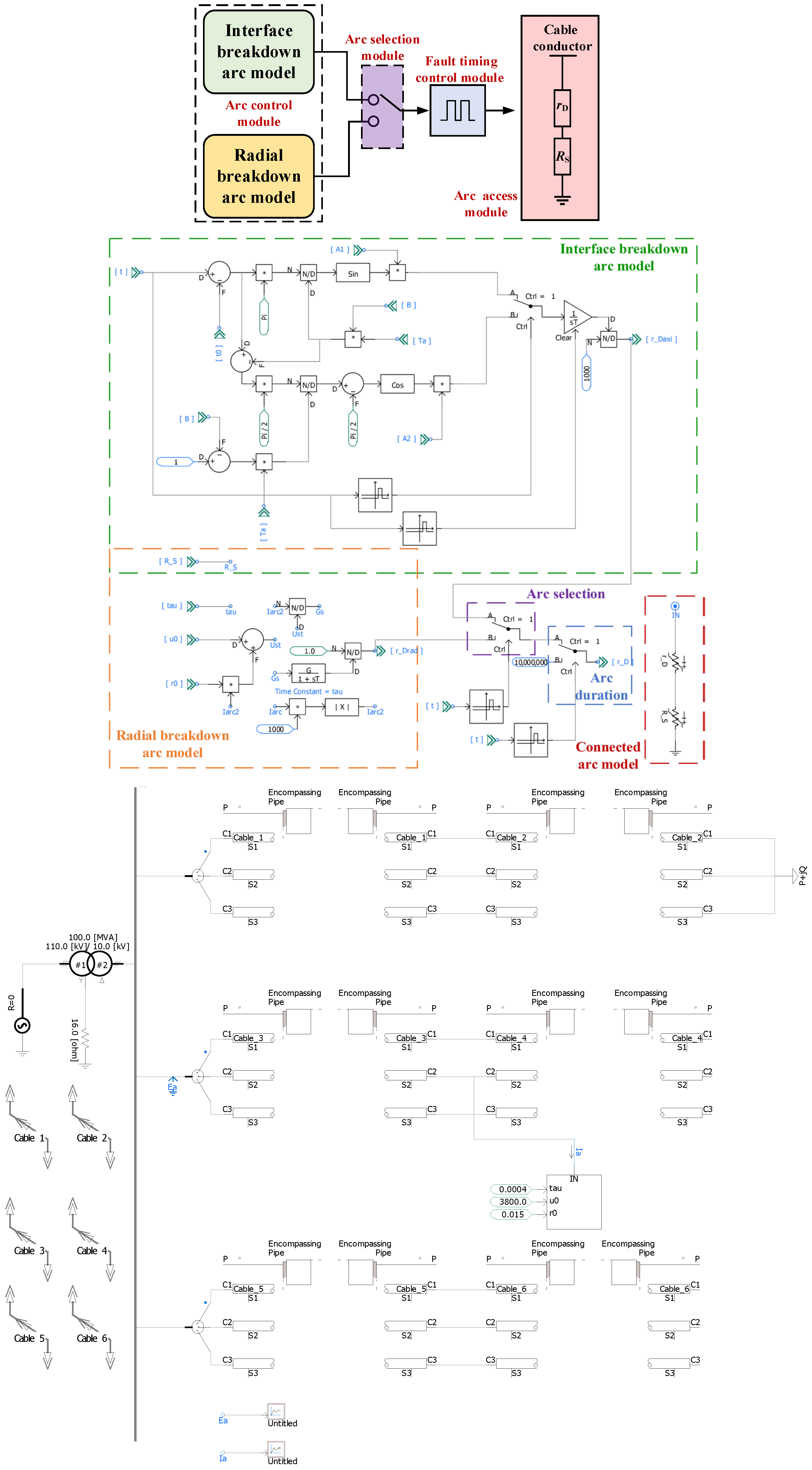
In light of the two kinds of arc models proposed above, a high-resistance to low-resistance grounding fault identification control model for cable joints is constructed in Figure 15,where the “*” is multiplication mark; the “#” is the mark for number; the arrows represents the direction of current; the colors represent different part of the circuit; the symbol represent different circuit component. This model is realized by PSCAD, which consists of the arc control module, the arc selection module, the fault timing control module, and the arc access module. Where the arc selection module controls the switching of arc types, the fault timing control module controls the initial arcing time and arc duration, which can be regulated by the switching functions of Equations (10) and (14); the arc access module is applied to connect the fault point of actual transmission lines for identifying the high-resistance to low-resistance grounding fault of cable joints. The details of the constructing method simulation software are exhibited.

This proposed model is based on arc characteristics of 10 kV cable joints at different evolution stages, which provides an effective means of identification for this critical fault type of cable joints. In distribution network systems, it is suggested that more attention should be paid to identifying high-resistance grounding faults of cable joints rather than ignoring such faults. Combined with the fault identification model with reference values and the actual monitored recording data in relay protection systems, it can be determined whether it is a cable joint fault. Once it is identified that the fault is caused by the cable joint, on the one hand, the faulty cable joint can be inspected and replaced in advance. On the other hand, the reclosing operation in the distribution network protection relay can be selectively restricted to avoid serious accidents caused by secondary impacts.

7. Conclusions

The complicated physical evolution of 10 kV cable joint faults is responsible for explosions or fire accidents in the distribution network system. Currently, there are no well-targeted measures to settle this typical fault.

(1)

The high-resistance to low-resistance grounding faults in 10 kV cable joints originates from XLPE-SiR insulation interface breakdown and further develops into radial breakdown of XLPE and SiR insulations under continuous insulation carbonization and electric field distortion. The equivalent electrical models are established to quantitatively interpret the whole evolution, which provides a solid physical and modeling foundation for relay protection modeling.

(2)

For the high-resistance grounding fault, an interface breakdown arc model based on segmented trigonometric function fitting is constructed, and the controlled parameter ranges of the arc model at different evolution stages are provided for reference. This realizes the quantitative description of time-varying arc characteristics induced by insulation state evolution, offering an effective early warning approach for the rapid identification of high-resistance grounding faults in relay protection.

(3)

For the low-resistance grounding fault, the Kizilcay arc model with classified control parameters under different stages is proposed, which can accurately describe the low-resistance arc characteristics. The model supports the rapid tripping action of relay protection devices.

In practical applications, the proposed cable joint fault identification and control model can be extended to higher voltage levels and applied to relay protection schemes in new-type power systems. It provides an effective identification approach for cable joint faults and further supports the prevention of catastrophic accidents.

References

1. Bonfiglio, A.; Brignone, M.; Delfino, F.; Procopio, R. Optimal control and operation of grid-connected photovoltaic production units for voltage support in medium-voltage networks. IEEE Trans. Sustain. Energy 2014, 5, 254–263. [Google Scholar] [CrossRef] [Scilit]
2. Abbas, G.; Alessandro, M.; Lorenzo, P.; Roberto, T. Effects of mechanical pressure on the tangent delta of mv cable joints. IEEE Trans. Instrum. Meas. 2019, 68, 2656–2658. [Google Scholar] [CrossRef] [Scilit]
3. Wu, J.; Mor, A.R.; Smit, J.J. The effects of superimposed impulse transients on partial discharge in xlpe cable joint. Int. J. Electr. Power Energy Syst. 2019, 110, 497–509. [Google Scholar] [CrossRef] [Scilit]
4. Hasheminezhad, M.; Ildstad, E. Application of contact analysis on evaluation of breakdown strength and pd inception field strength of solid-solid interfaces. IEEE Trans. Dielectr. Electr. Insul. 2012, 19, 1–7. [Google Scholar] [CrossRef] [Scilit]
5. Zhao, Y.; Liu, G.; Huang, C.; Xu, Z.; Zhou, W. Evolution of grounding failure-insulation failure of 10 kV cable joints: Prerequisites of an explosion in enclosed cable trench. IET Gener. Transm. Distrib. 2023, 17, 3751–3762. [Google Scholar] [CrossRef] [Scilit]
6. Hu, R.; Liu, G.; Huang, C.; Xu, Z.; Zhou, W. Power cable fired by transient arcing below the action value of relay protection: An analysis of a medium-voltage cable joint breakdown fault. Eng. Fail. Anal. 2023, 145, 107028. [Google Scholar] [CrossRef] [Scilit]
7. Pompili, M.; Calcara, L.; D’Orazio, L.; Ricci, D.; He, H. Joints defectiveness of mv underground cable and the effects on the distribution system. Electr. Power Syst. Res. 2021, 192, 107004. [Google Scholar] [CrossRef] [Scilit]
8. Grzegorz, W. Determining location of voltage fluctuation source in radial power grid. Electr. Power Syst. Res. 2021, 180, 106069. [Google Scholar]
9. Xu, X.; Hu, W. Modeling and simulation of arc grounding fault of middle and low voltage distribution network based on atp-emtp. J. Comput. Methods Sci. Eng. 2020, 20, 1–10. [Google Scholar] [CrossRef] [Scilit]
10. Yu, R.; Fu, Z.; Wang, Q.; Sun, S.; Chen, X. Modeling and simulation analysis of single phase arc grounding fault based on MATLAB. In Proceedings of 2011 International Conference on Electronic & Mechanical Engineering and Information Technology; IEEE: New York, NY, USA, 2011; pp. 4607–4610. [Google Scholar]
11. Jalil, M.; Samet, H.; Ghanbari, T.; Tajdinian, M. An enhanced cassie-mayr-based approach for dc series arc modeling in pv systems. IEEE Trans. Instrum. Meas. 2021, 70, 9005710. [Google Scholar] [CrossRef] [Scilit]
12. Guardado, J.L.; Maximov, S.G.; Melgoza, E.; Naredo, J.L.; Moreno, P. An improved arc model before current zero based on the combined mayr and cassie arc models. IEEE Trans. Instrum. Meas. 2005, 20, 138–142. [Google Scholar] [CrossRef] [Scilit]
13. Yang, F.; Tang, Z.; Shen, Y.; Su, L.; Yang, Z. Zhichun Parameter Determination Method of Cassie-Mayr Hybrid Arc Model Based on Magnetohydrodynamics Plasma Theory. Front. Energy Res. 2022, 10, 808289. [Google Scholar]
14. Kuffel, E.; Zaengl, W.S. High-Voltage Engineering: Fundamentals; Pergamon Press: Oxford, UK, 2000. [Google Scholar]
15. Wang, H.; Wang, X.; Chen, F. Effect of silicone grease swelling with corona aging on properties of silicone rubber and interfacial charge characteristics between XLPE and SiR. High Volt. Eng. 2020, 46, 1639–1648. (In Chinese) [Google Scholar]
16. Wei, Y.; Liu, M.; Han, W.; Li, G.; Lei, Q. Charge injection characteristics of semi-conductive composites with carbon black-polymer for hvdc cable. Polymers 2019, 11, 1134. [Google Scholar] [CrossRef] [Scilit] [PubMed]
17. Li, L.; Li, Y.; Zhou, X.; Yang, Z.; Wang, K. Modeling of Internal Multiform Intermittent Arc Fault for 10kV XLPE Cable. Trans. China Electrotech. Soc. 2022, 37, 6104–6115. (In Chinese) [Google Scholar]
18. Kizilcay, M.; Pniok, T. Digital simulation of fault arcs in power systems. Eur. Trans. Electr. Power 1991, 1, 55–60. [Google Scholar] [CrossRef] [Scilit]
19. Zhang, W.; Xiao, X.; Zhou, K. Multicycle incipient fault detection and location for medium voltage underground cable. IEEE Trans. Power Deliv. 2016, 32, 1450–1459. [Google Scholar] [CrossRef] [Scilit]
20. Wang, Y.; Lu, H.; Xiao, X.; Yang, X.; Zhang, W. Cable incipient fault identification using restricted boltzmann machine and stacked autoencoder. IET Gener. Transm. Distrib. 2020, 14, 1242–1250. [Google Scholar] [CrossRef] [Scilit]
Figure 1. A statistical diagram of the types of faults in the distribution network cable system.
Energies 19 01996 g001
Figure 2. Schematic diagram of the discharge paths of the cable joint 3. Physical process of interface breakdown.
Energies 19 01996 g002
Figure 3. Physical evolution diagram of discharge behaviors in faulty cable joints.
Energies 19 01996 g003
Figure 4. Circuit model based on the physical structure of the cable joint.
Energies 19 01996 g004
Figure 5. Simulated XLPE-SiR insulation interface sample with water film.
Energies 19 01996 g005
Figure 6. The schematic diagram of the experiment.
Energies 19 01996 g006
Figure 7. Evolution of interface breakdown waveforms of ui and ib in experiment tests. (a) Initial state; (b) state 1; (c) state 2; (d) state3; (e) state4.
Energies 19 01996 g007
Figure 8. The SiR morphology caused by interface breakdown at different stages. (a) state 1; (b) state 2; (c) state3; (d) state4.
Energies 19 01996 g008
Figure 9. Interface breakdown circuit model of cable joints.
Energies 19 01996 g009
Figure 10. Constructing method of interface breakdown arc resistance model.
Energies 19 01996 g010
Figure 11. Evolution of ui and ig obtained by fault-recording data. (a) Initial stage; (b) Early stage; (c) Intermediate stag; (d) Last stage.
Energies 19 01996 g011
Figure 12. Radial breakdown circuit model of cable joints.
Energies 19 01996 g012
Figure 13. The fault line topology with Kizilcay’s arc model constructed by PSCAD.
Energies 19 01996 g013
Figure 14. Simulated results under different stages of radial breakdown evolution. (a) Initial stage; (b) Early stage; (c) Intermediate stage; (d) Last stage.
Energies 19 01996 g014
Figure 15. Implementation of fault identification control model of cable joints.
Energies 19 01996 g015