Imbalance-Aware Spatiotemporal Load Forecasting via Cluster-Weighted State Space Modeling

Abstract

Electrical load time series exhibit strong heterogeneity across daily patterns driven by calendar effects and behavioral variability, leading many forecasting models to favor dominant weekday profiles while degrading on weekends, holidays, and transition days. This paper proposes an imbalance-aware spatiotemporal forecasting framework via a cluster-conditioned state space model. Daily load patterns are identified via time-series clustering and incorporated as conditioning covariates within a sequence-continuous selective state space models (Mamba), preserving temporal coherence without explicit sequence partitioning. A cluster-weighted training objective further mitigates pattern imbalance while avoiding future-information leakage. The resulting cluster-conditioned Time Series Mamba (TSMamba) consistently improves forecasting robustness across both frequent and infrequent profiles, achieving weighted absolute percentage error (WAPE) reductions of approximately 15% on weekdays, 42% on weekends, and 39% on holidays relative to the vanilla TSMamba, with similar gains in mean absolute error (MAE) and coefficient of variation of the root mean square error (CVRMSE). These results demonstrate that conditioning state dynamics on latent load patterns yields stable and computationally efficient short-term load forecasts under profile transitions.

1. Introduction

Short-term load forecasting (STLF) is a foundational task in power system operation, directly supporting unit commitment, reserve scheduling, market clearing, and reliability assessment. The increasing electrification of end-use sectors, particularly the rapid adoption of electric vehicles, is expanding the operational scope of load forecasting in power system planning and market operation. Electric vehicle charging and data centers introduces demand patterns that are highly time-dependent and often irregular, increasing uncertainty in system load behavior. At the same time, emerging electricity and carbon market mechanisms require reliable demand forecasts to support coordinated energy and emissions management. Recent studies on grid integration of electric vehicles within electricity and carbon markets highlight that forecasting models must remain reliable under evolving demand regimes driven by electrification, flexible loads and climate-dependent demand [1]. These developments reinforce the need for forecasting frameworks capable of maintaining accuracy across heterogeneous and shifting load patterns. Empirical studies consistently show that daily demand profiles vary substantially between weekdays, weekends, holidays, and transition days, reflecting underlying behavioral and operational shifts [2,3,4,5,6].

Despite this heterogeneity, most learning-based forecasting models are trained on datasets dominated by weekday observations, biasing parameter optimization toward typical weekday dynamics [7,8]. As a result, infrequent load profiles such as weekends, holidays, and transition days are underrepresented during training, leading to systematic error amplification during these regimes [4,5]. Such degradation is particularly problematic for operational tasks including system marginal price (SMP) estimation, congestion management, and contingency planning [6,9].

Recent advances in deep learning have substantially improved the ability of forecasting models to capture nonlinear dependencies and complex seasonal structures in electrical load time series [8,10,11]. However, these improvements do not inherently resolve the imbalance problem. Even highly expressive architectures tend to minimize average forecasting error over dominant patterns, implicitly sacrificing performance on rare but structurally distinct demand profiles such as weekends and holidays [5,6]. This observation motivates the need for forecasting frameworks that explicitly account for pattern imbalance while preserving the sequential structure of the time series.

A substantial body of literature has explored clustering-based approaches to address load heterogeneity by separating historical load profiles into distinct consumption patterns. While clustering improves interpretability and local pattern modeling, most existing approaches partition the time series into independent subsets and train separate models per cluster. This strategy fundamentally disrupts temporal continuity, as long-range dependencies across clusters are broken once the sequence is segmented. Furthermore, assigning future observations to clusters often requires ex-ante classification, which introduces information leakage or relies on auxiliary classifiers that themselves incur uncertainty.

Recent sequence-to-sequence clustering (S2S) frameworks attempt to reconstruct temporal dependency after clustering by re-ordering cluster members into surrogate sequences [4,6,12]. Although effective in improving accuracy, these approaches still rely on cluster-specific models, increasing system complexity and complicating deployment in operational environments. At the same time, emerging long-range sequence models, including state space models (SSMs) and structured sequence architectures, provide strong guarantees on temporal continuity and stability [13,14,15]. However, these models are typically trained under uniform loss formulations that remain vulnerable to data imbalance.

Consequently, a gap remains for a unified, sequence-preserving forecasting framework that (i) explicitly accounts for pattern imbalance, (ii) avoids cluster-specific model fragmentation, and (iii) ensures leak-free training and inference. Addressing this gap is the focus of this work.

Short-term load forecasting has been extensively studied using both statistical and deep learning approaches. Classical methods such as autoregressive integrated moving average (ARIMA) and linear regression provide interpretable baselines but struggle to capture nonlinear dynamics and nonstationary demand patterns. As a result, deep learning models have become dominant [8].

Hybrid convolutional neural network (CNN) with a recurrent neural network (RNN), (CNN–RNN) architectures are widely adopted to jointly model local load-shape characteristics and temporal dependencies. The work by [6] propose a CNN with gated recurrent unit (GRU), (CNN–GRU) framework for short-term load forecasting that demonstrates improved accuracy over standalone cluster models. Similarly, ref. [16] employ a CNN with long short-term memory architecture (LSTM), (CNN–LSTM) architecture to capture temporal features under varying load conditions. While these models improve average forecasting accuracy, their training objectives remain dominated by frequent weekday observations, leading to degraded performance on weekends and holidays.

Transformer-based models further enhance long-range dependency modeling. Ref. [11] introduce an attention-based forecasting framework that improves long-horizon accuracy, while [10] apply temporal attention mechanisms to load forecasting with promising results. However, these models primarily optimize global loss metrics and do not explicitly address demand pattern imbalance. Consequently, performance improvements are unevenly distributed across load profiles, with minority patterns receiving limited attention during training.

In contrast, the present work focuses explicitly on imbalance-aware learning within a unified model, rather than relying on increased model expressiveness alone.

Load profile analysis has long been used to characterize demand heterogeneity through clustering and classification. Ref. [4] apply k-means clustering to daily load curves to identify typical consumption patterns and train separate forecasting models for each cluster. Ref. [12] similarly employ k-medoids clustering to segment daily load profiles, reporting improved forecasting accuracy within each cluster.

More recent studies adopt shape-based clustering techniques to better capture load profile similarity. Ref. [17] introduce Shape dynamic time warping (DTW) clustering to group daily load profiles based on shape similarity rather than magnitude. Ref. [18] extend this idea using spatiotemporal graph embeddings combined with load-shape clustering to improve forecasting accuracy across regions.

Most notably, Ref. [19] propose a spatiotemporal sequence-to-sequence clustering framework that reconstructs cluster-specific sequences to preserve temporal order within clusters. While this approach significantly improves accuracy and computational efficiency, it still relies on training separate models per cluster, thereby fragmenting the original time series and complicating inference.

Unlike these approaches, the proposed method does not partition the time series. Instead, DTW-based clustering is used solely to derive load pattern features, which condition a single sequence-continuous SSM.

SSMs provide a principled framework for modeling temporal dynamics via latent state evolution. Ref. [20] employ ConvLSTM architectures that implicitly encode state transitions for load forecasting, demonstrating improved long-term dependency modeling compared to standard RNNs. Ref. [21] incorporate Hawkes-process-inspired temporal decoders to capture self-exciting load behaviors. Ref. [22] introduce gated temporal fusion mechanisms to improve temporal representation learning. While these models exhibit strong performance, their state representations remain implicit, and none explicitly integrate pattern-aware conditioning or imbalance-aware objectives.

Importantly, recent structured state space approaches employ Mamba [13,14,15]. Mamba is a structured SSM that replaces attention with selective state updates, enabling linear-time sequence modeling while preserving long-range temporal dependencies through explicit state evolution. While preserving temporal continuity and improving scalability, Mamba remain optimized under uniform loss formulations and do not address demand profile imbalance or information leakage arising from load-pattern identification.

The present work addresses this gap by embedding pattern-aware conditioning and cluster-weighted loss directly into a unified SSM framework.

Imbalance-aware learning is well studied in classification but remains underexplored in time-series forecasting. In the context of load forecasting, imbalance is typically handled heuristically. Ref. [5] train separate forecasting models for holidays and non-holidays, reporting improved holiday accuracy at the cost of increased model complexity and reduced temporal continuity. Ref. [11] incorporate weekday/weekend indicators as auxiliary inputs, while [23] propose ensemble weighting schemes to emphasize specific load patterns. However, these methods do not alter the underlying optimization objective and therefore fail to correct gradient dominance induced by frequent patterns.

Critically, none of the reviewed studies employ cluster-frequency–based loss reweighting, nor do they formally address information leakage arising from pattern identification. As highlighted in the discussions above [5,11,23], imbalance is often described but rarely addressed at the learning-objective level.

The works discussed above are summarized in

Table 1. Comparison of Related Work.

Paper	Temporal Continuity Preserved	Imbalance Explicitly Addressed	Leakage Explicitly Avoided	Model Class
Proposed (this work)	✓	✓ (loss-level)	✓ (leak-free)	Cluster-conditioned SSM (Mamba)
Wang et al. [15]	✓	✗	✓	Structured SSM (Mamba)
Si et al. [24]	✓	❍ (distribution mismatch)	✓	Robust co-modeling
Masood et al. [9]	✓	❍ (probabilistic focus)	✓	Quantile LSTM
Haq & Ni [23]	✓	❍ (ensemble weighting)	✓	ENN ensemble
Zhou et al. [11]	✓	❍ (calendar indicators)	✓	Transformer STGNN
Acquah et al. [6]	✓	❍ (cluster partitioning)	✓	S2S clustering + CNN–GRU
Hasanat et al. [16]	✓	✗	✓	CNN–LSTM
Jalalifar et al. [20]	✓	✗	✓	ConvLSTM
Jiang et al. [22]	✓	✗	✓	STFGCN
Zhao et al. [10]	✓	✗	✓	Transformer + attention
Pan et al. [19]	❍ (within clusters only)	✗	✗	S2S clustering + DL
Luo et al. [5]	✗ (separate profiles)	❍ (holiday split)	❍	Profile-specific models
Khan et al. [12]	✗ (cluster partitioning)	❍ (cluster separation)	✗	K-medoids + DL ensemble
Syed et al. [25]	✗	❍ (pattern recognition)	✗	Clustering + DNN
Kouloumpris et al. [26]	✗	❍	✗	Clustered hybrid DL
Dou et al. [18]	✗	✗	✗	Spatiotemporal clustering + attention
Wei et al. [27]	✗	✗	✗	LDTW + GCN
Wu et al. [17]	✗	✗	✗	K-shape + GCN
Feng & Wang [4]	✗ (cluster-wise models)	✗	✗	K-means + separate regressors

Legend: ✓ = explicitly satisfied; ❍ = partially addressed (heuristics or limited scope); ✗ = not addressed.

to highlight that existing short-term load forecasting approaches address demand heterogeneity in a fragmented manner. Clustering-based methods improve interpretability and within-pattern accuracy but rely on hard time-series partitioning, which disrupts temporal continuity and often introduces information leakage when profile identification depends on full-day load profiles. In contrast, sequence-preserving deep learning models, such as CNN–RNN hybrids, transformer architectures, and spatiotemporal networks, maintain temporal structure but are trained under uniform loss objectives that bias learning toward dominant weekday profiles, resulting in persistent performance degradation during weekends, holidays, and transition periods. Although some studies incorporate calendar indicators, profile separation, or ensemble weighting, these strategies treat imbalance heuristically and do not correct gradient dominance at the optimization level. Moreover, structured SSMs have not been systematically combined with load-shape profile information or imbalance-aware training objectives in prior work.

These limitations motivate the proposed framework, which integrates k-means based load pattern characterization as causal conditioning features within a single sequence-continuous SSM and introduces a cluster-weighted loss to explicitly address profile imbalance while avoiding information leakage.

The main contributions of this paper are:

• An imbalance-aware TSMamba forecasting framework that preserves temporal continuity while improving robustness across load patterns.
• A time-series clustering strategy for daily load pattern characterization aligned with calendar structure and load-shape similarity.
• A cluster-conditioned TSMamba that incorporates load pattern information as causal conditioning covariates.
• A cluster-weighted training objective that mitigates pattern imbalance without future-information leakage.

The rest of the contents are arranged as follows: Section 2 presents the proposed imbalance-aware cluster-conditioned TSMamba framework, including the problem formulation, architecture, and cluster-weighted training objective. Section 3 describes the experimental setup, including data preprocessing, load pattern characterization, and implementation details. Section 4 reports the forecasting results and discusses performance across load patterns and transition robustness. Finally, Section 5 concludes the paper and outlines future research directions.

2. Proposed Methodology

2.1. Problem Definition

Short-term load forecasting is formulated as a supervised multivariate sequence-to-sequence prediction problem over a continuous time series. Let

$${\{y_t,x_t\}}_{t=1}^T$$

denote historical electrical load observations $y_t\in \mathbb{R}$ and associated exogenous variables $x_t\in {\mathbb{R}}^d$, observed at a fixed temporal resolution (e.g., hourly). The exogenous variables include calendar indicators and engineered temporal features that are causally available at time t.

Given a historical lookback window of length L, the forecasting objective is to learn a mapping

$${\widehat{y}}_{t+1:t+H}=f\left(y_{t-L+1:t},x_{t-L+1:t}\right),$$

which predicts the future load trajectory over a horizon H. The forecasting function $f(·)$ is parameterized by a sequence model that operates on the input as a single continuous sequence, rather than partitioning it into disjoint segments, thereby preserving temporal coherence across the forecasting horizon.

This formulation aligns with recent SSM–based time-series forecasting approaches, which emphasize long-range dependency modeling through latent state evolution. Such continuity is particularly important for electrical load data, where demand exhibits strong temporal persistence and dependencies spanning multiple days.

In practical settings, however, the empirical distribution of load patterns is highly imbalanced: weekday demand profiles dominate historical data, while weekends, holidays, and transition days occur infrequently. Training under a uniform loss objective therefore biases models toward dominant patterns, leading to degraded performance during irregular or transition-driven regimes. This work therefore defines the forecasting problem under a single continuous sequence, where pattern information and imbalance are addressed within the model and training objective rather than through sequence partitioning or pattern-specific models, consistent with modern state space–based time-series formulations.

2.2. Framework Overview

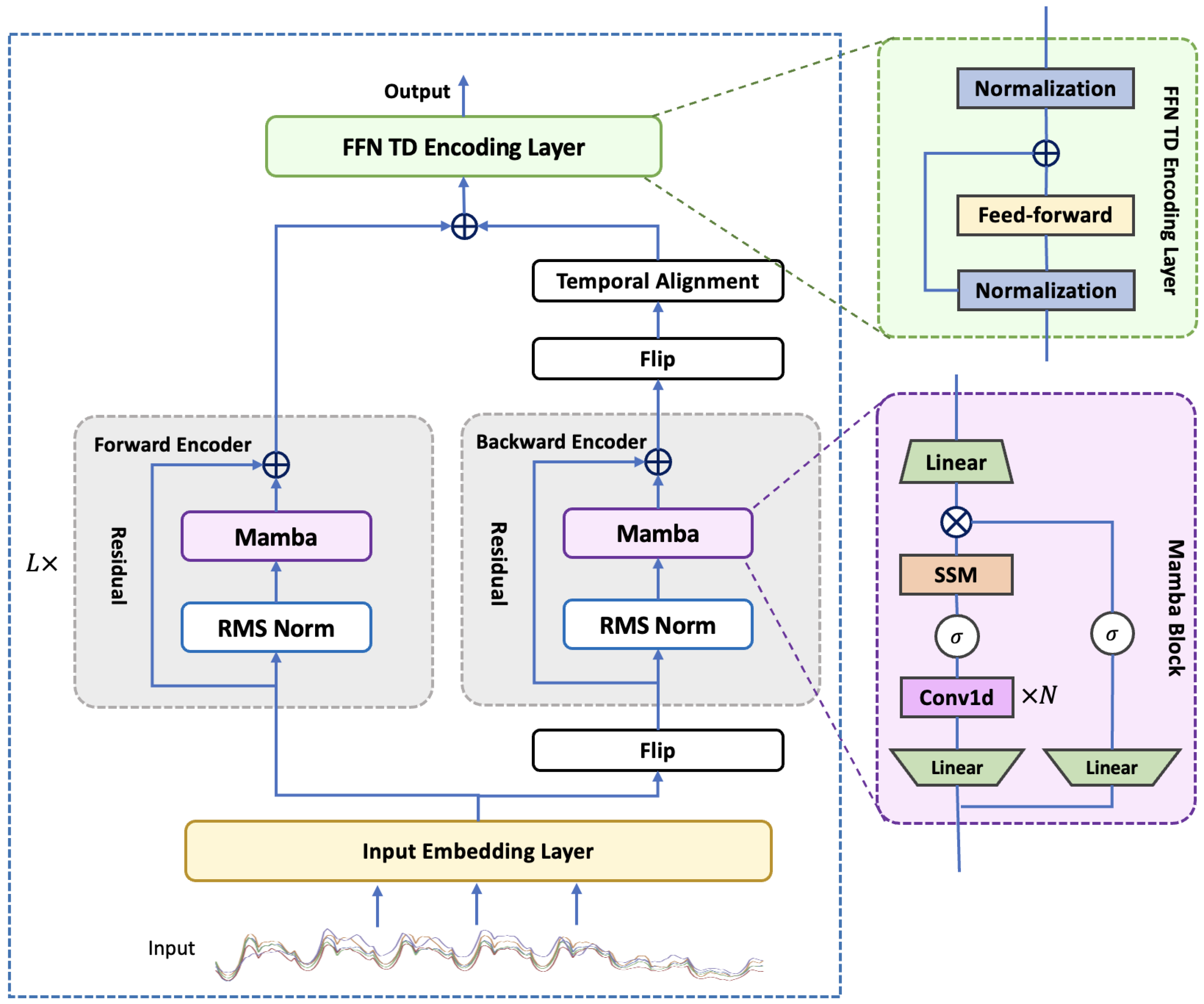
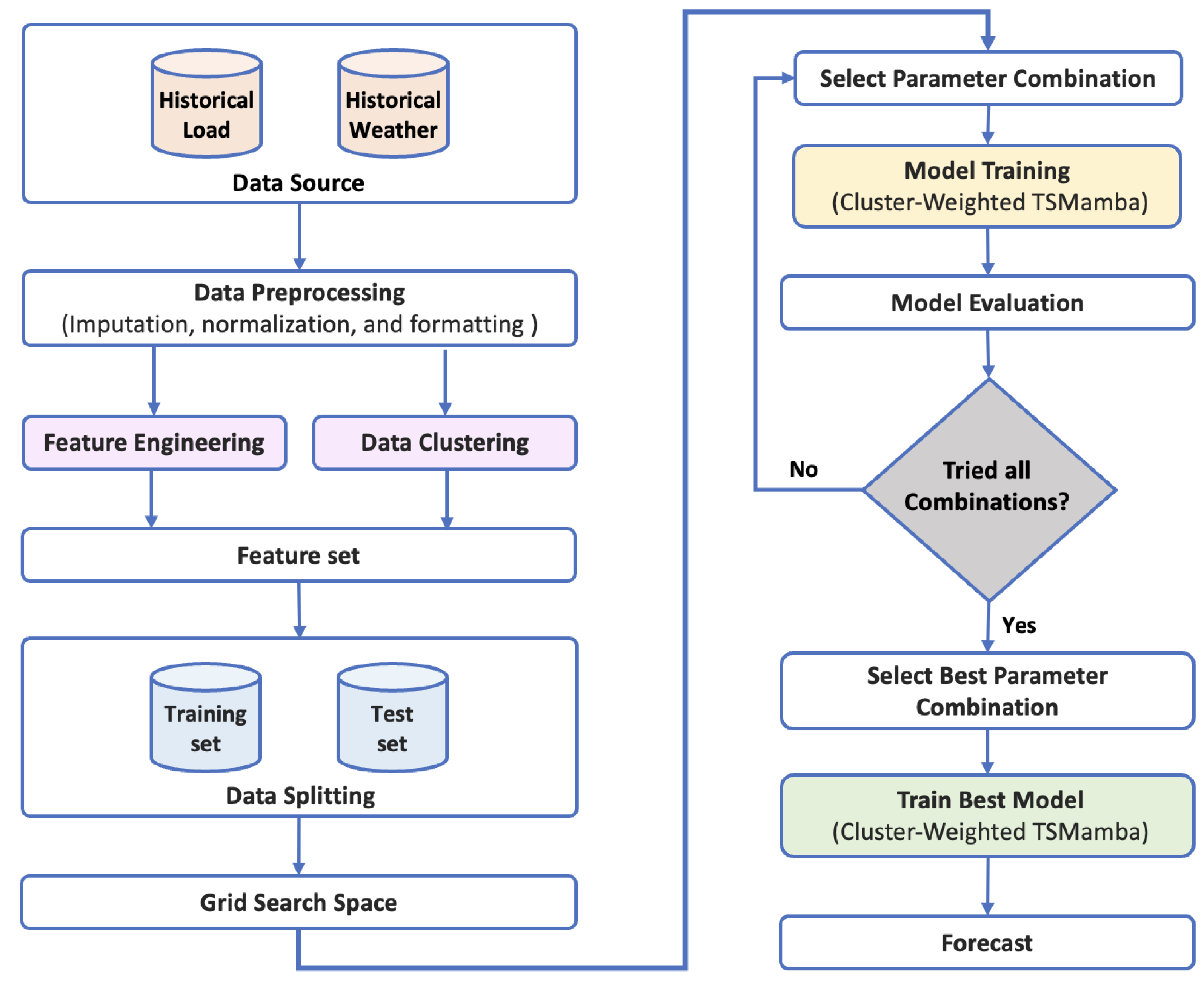
The proposed forecasting framework builds on the Time-Series Mamba (TSMamba) architecture [15], leveraging selective state space modeling to achieve efficient long-range sequence modeling while explicitly addressing load-pattern heterogeneity and data imbalance. Figure 1 illustrates the overall structure of the proposed TSMamba-based forecasting framework with load pattern conditioning and cluster-weighted training.

Given a multivariate historical load sequence and associated exogenous inputs, the model operates on a single continuous sequence without temporal partitioning. The input is first mapped into a latent representation through an input embedding layer, which projects raw load observations and contextual features into a shared feature space suitable for sequence modeling. This embedding preserves the temporal order of the sequence and serves as the input to a stack of TSMamba blocks.

Each TSMamba block consists of two complementary components designed to capture distinct aspects of time-series structure. First, a bidirectional Mamba-based encoding module models long-range temporal dependencies through selective state space dynamics. Forward and backward Mamba encoders process the sequence in opposite temporal directions, enabling the model to capture both causal and anti-causal temporal patterns. The backward representation is temporally flipped and aligned with the forward stream, and the two representations are fused through residual connections to form a unified sequence representation. This bidirectional design mitigates the unidirectional limitation of standard Mamba blocks while preserving near-linear computational complexity.

Second, a feed-forward temporal dependency (FFN-TD) encoding layer refines the fused representation by modeling local temporal interactions and nonlinear dependencies. The FFN-TD layer follows a normalization–feed-forward–normalization structure, ensuring stable training and effective feature transformation. Residual connections are employed throughout the block to maintain information flow across layers and support deep stacking of TSMamba modules.

To incorporate heterogeneous daily load patterns without fragmenting the sequence, load pattern information obtained from offline clustering is injected into the model as conditioning covariates. Pattern descriptors are aligned with each time step and used to modulate the internal state evolution of the Mamba-based state space components. This conditioning allows the latent dynamics to adapt to structurally distinct demand patterns, such as weekdays, weekends, holidays, and transition days, while preserving temporal continuity across pattern boundaries.

The output of the stacked TSMamba blocks is passed through a projection layer that maps latent representations to future load trajectories over the prediction horizon. During training, an imbalance-aware learning objective is employed in which loss contributions are reweighted according to the empirical frequency of load patterns. This cluster-weighted training strategy ensures that infrequent but operationally critical patterns exert sufficient influence on parameter updates, without requiring pattern-specific models or future-information leakage.

Overall, the proposed framework integrates selective state space modeling, bidirectional temporal encoding, load-pattern conditioning, and cluster-weighted optimization within a unified sequence-continuous architecture. This design enables robust and computationally efficient short-term load forecasting across heterogeneous demand patterns, making it well suited for operational power system applications.

2.3. TSMamba Block Architecture

The core building block of the proposed framework is the TSMamba block, which combines bidirectional selective state space modeling with feed-forward temporal dependency encoding. Each block operates on a continuous latent sequence and is designed to capture long-range temporal dynamics while maintaining computational efficiency [13,14].

Let $Z={\left\{z_t\right\}}_{t=1}^T$ denote the input sequence to a TSMamba block, where $z_t\in {\mathbb{R}}^d$ represents the embedded load and exogenous features at time t. Prior to state evolution, the input is normalized using RMS normalization,

$${\tilde{z}}_t=\mathrm{RMSNorm}\left(z_t\right).$$

(1)

2.3.1. Bidirectional Mamba State Evolution

To capture both forward and backward temporal dependencies, the TSMamba block employs two parallel Mamba encoders. The forward encoder processes the sequence in causal order,

$$h_{t+1}^{\to }=\mathcal{M}\left(h_t^{\to },{\tilde{z}}_t;{\theta }^{\to }\right),$$

(2)

where $\mathcal{M}(·)$ denotes the selective state space update implemented by the Mamba module, and $h_t^{\to }$ is the forward latent state.

Similarly, a backward Mamba encoder processes the reversed sequence,

$$h_{t-1}^{\leftarrow }=\mathcal{M}\left(h_t^{\leftarrow },{\tilde{z}}_t;{\theta }^{\leftarrow }\right).$$

(3)

The backward output is temporally flipped to align with the forward representation,

$${\widehat{h}}_t^{\leftarrow }=\mathrm{Flip}\left(h_t^{\leftarrow }\right).$$

(4)

The aligned forward and backward representations are fused through residual summation,

$$u_t=z_t+h_t^{\to }+{\widehat{h}}_t^{\leftarrow },$$

(5)

ensuring that both causal and anti-causal temporal information contribute to the updated sequence representation.

2.3.2. Selective State Space Computation

Within each Mamba encoder, state evolution follows a selective state space formulation. For each channel, the latent state evolves as

$$s_{t+1}=A\left(c_t\right)s_t+B\left(c_t\right)\sigma \left(W_u{z}_t\right),$$

(6)

$$y_t=C\left(c_t\right)s_t+D\left(c_t\right)z_t,$$

(7)

where $s_t$ denotes the internal state, $\sigma (·)$ is a gating nonlinearity, and $(A,B,C,D)$ are pattern-conditioned state space parameters. The conditioning variable $c_t$ represents the load pattern descriptor associated with time t, allowing the state transition dynamics to adapt to heterogeneous demand profiles without sequence partitioning.

2.3.3. Feed-Forward Temporal Dependency Encoding

Following bidirectional state fusion, the representation is refined using a feed-forward temporal dependency (FFN-TD) encoding layer. This layer applies a position-wise nonlinear transformation with residual connection,

$$v_t=u_t+\mathrm{FFN}\left(\mathrm{Norm}\left(u_t\right)\right),$$

(8)

where the FFN consists of two linear transformations with an activation function,

$$\mathrm{FFN}\left(x\right)=W_2\varphi \left(W_{1}x\right).$$

(9)

The FFN-TD layer enhances local temporal interactions and nonlinear feature mixing, complementing the long-range modeling capability of the state space components.

2.3.4. Block Output

The output of the TSMamba block is the sequence ${\left\{v_t\right\}}_{t=1}^T$, which serves as input to the next stacked block or to the final forecasting head. Residual connections, normalization layers, and selective state transitions collectively ensure stable training, efficient gradient propagation, and scalability to long lookback windows.

By stacking multiple TSMamba blocks, the proposed framework incrementally refines temporal representations while preserving sequence continuity and adapting latent dynamics to heterogeneous load patterns.

2.4. Cluster-Weighted Training Objective

In practical load forecasting datasets, the empirical distribution of daily load patterns is highly imbalanced, with weekday patterns dominating the training samples. To prevent the optimization process from being biased toward these frequent patterns, the proposed framework employs a cluster-weighted training objective.

Let $\ell (y_t,{\widehat{y}}_t)$ denote a pointwise forecasting loss, such as mean absolute error or squared error. The overall training objective is defined as

$$\mathcal{L}=\sum _{t=1}^T{w}_{c_t}\ell \left(y_t,{\widehat{y}}_t\right),$$

(10)

where $w_{c_t}$ is a nonnegative weight associated with the load pattern $c_t$. The weights are chosen to be inversely proportional to the empirical frequency of each pattern,

$$w_c\propto {\displaystyle \frac{1}{\mathrm{freq}\left(c\right)}},$$

(11)

and normalized to ensure numerical stability during training.

This weighting scheme amplifies gradient contributions from infrequent but operationally critical patterns, such as weekends, holidays, and transition days, without oversampling or duplicating data. Unlike pattern-specific model training, cluster-weighted optimization preserves a single unified model and maintains temporal coherence across the full sequence.

Because pattern assignments and cluster frequencies are computed offline using historical data only, the weighting mechanism does not rely on future information and remains valid during inference. The cluster-weighted loss therefore complements the pattern-conditioned state dynamics by addressing imbalance at the optimization level, ensuring that the learned parameters are robust across both dominant and rare load patterns.

Together, cluster-conditioned state evolution and cluster-weighted training form a coherent imbalance-aware learning strategy that operates entirely within a sequence-continuous forecasting framework.

Gradient Interpretation of Cluster Weighting

The effect of cluster-weighted training can be made explicit by examining the gradients that drive parameter updates. Let $\theta$ denote the parameters of the forecasting model (including the TSMamba encoder, the cluster-conditioned state space components, and the output head), and define the weighted empirical risk

$$\mathcal{L}\left(\theta \right)=\sum _{t=1}^T{w}_{c_t}\ell \left(y_t,{\widehat{y}}_t\left(\theta \right)\right).$$

(12)

The gradient of the objective is

$${\nabla }_{\theta }\mathcal{L}\left(\theta \right)=\sum _{t=1}^T{w}_{c_t}{\nabla }_{\theta }\ell \left(y_t,{\widehat{y}}_t\left(\theta \right)\right).$$

(13)

Grouping terms by load pattern (cluster) $c\in \{1,\dots ,K\}$ yields

$${\nabla }_{\theta }\mathcal{L}\left(\theta \right)=\sum _{c=1}^K{w}_c\sum _{t\in {\mathcal{T}}_c}{\nabla }_{\theta }\ell \left(y_t,{\widehat{y}}_t\left(\theta \right)\right),$$

(14)

where ${\mathcal{T}}_c=\{t:c_t=c\}$ denotes the set of time indices assigned to cluster c and $w_c$ is the corresponding cluster weight.

Let $n_c=\left|{\mathcal{T}}_c\right|$ and $\mathrm{freq}\left(c\right)=n_c/T$. If the weights are chosen as

$$w_c={\displaystyle \frac{\alpha }{n_c}},$$

(15)

for some scaling constant $\alpha >0$, then (14) becomes

$${\nabla }_{\theta }\mathcal{L}\left(\theta \right)=\alpha \sum _{c=1}^K{\displaystyle \frac{1}{n_c}}\sum _{t\in {\mathcal{T}}_c}{\nabla }_{\theta }\ell \left(y_t,{\widehat{y}}_t\left(\theta \right)\right)=\alpha \sum _{c=1}^K{\overline{g}}_c\left(\theta \right),$$

(16)

where

$${\overline{g}}_c\left(\theta \right)={\displaystyle \frac{1}{n_c}}\sum _{t\in {\mathcal{T}}_c}{\nabla }_{\theta }\ell \left(y_t,{\widehat{y}}_t\left(\theta \right)\right)$$

(17)

is the average per-sample gradient contributed by cluster c. Equation (16) shows that inverse-count weighting approximately equalizes the influence of each load pattern on the update direction by summing cluster-average gradients rather than allowing frequent clusters to dominate via larger sample counts.

$$w_c=\mathrm{freq}{\left(c\right)}^{-\gamma },\gamma \in [0,1].$$

(18)

More generally, using (18) provides a continuous control over the trade-off between overall accuracy (small $\gamma$) and minority-pattern emphasis (large $\gamma$). When $\gamma =0$, the objective reduces to uniform empirical risk minimization; when $\gamma =1$, the gradient contributions tend toward equalized cluster influence as in (16).

Equation (10) defines the base cluster weight $w_c$ derived from empirical cluster frequencies. Equation (15) represents the inverse-frequency weighting obtained when $\gamma =1$, while (18) generalizes this formulation by introducing the exponent $\gamma$, which provides continuous control over the degree of imbalance correction during training.

Cluster frequencies are estimated from historical training data to address imbalance within the observed dataset rather than track long-term behavioral changes in real time. In operational settings, models are typically retrained periodically as new data become available, allowing cluster assignments and frequency weights to update as consumption patterns evolve.

The cluster-weighted learning does not alter the model architecture or require cluster-specific predictors. Instead, it modifies the optimization geometry so that parameter updates reflect a more balanced objective across heterogeneous load patterns, improving robustness on infrequent patterns without sacrificing temporal continuity.

3. Experimental Setup

3.1. Dataset Description and Preprocessing

Empirical evaluation is conducted using a nationwide hourly electricity demand dataset obtained from the Korea Power Exchange (KPX), Naju, South Korea [28], covering the period from January 2015 to February 2022. After imputing days with incomplete or invalid records, the dataset comprises 2606 complete daily load profiles, each consisting of 24 hourly demand observations. The raw time series is chronologically sorted and cleaned to eliminate duplicated timestamps and missing values, yielding a fully observed sequence suitable for clustering and forecasting.

To account for exogenous drivers of demand variability, an hourly weather dataset for the same period is collected via the Korea Public Data Portal API, Naju, South Korea [29]. Weather data are obtained from the national meteorological weather stations (Seoul, Daegu, and Busan) and spatially aggregated to the country level to match the load footprint. The weather variables used include temperature and humidity.

Temperature and humidity were selected because they are the primary meteorological drivers of electricity demand in the dataset, mainly through their effect on heating and cooling consumption. The proposed framework does not restrict the choice of exogenous inputs, and additional meteorological or system features can be incorporated without modifying the model architecture. All weather features are temporally aligned with the load measurements and incorporated as additional covariates in the forecasting models.

The data were acquired in batches through an application programming interface, which introduces occasional irregularities dominated by missing timestamps caused by transmission gaps and timestamp misalignment. In the examined dataset, missing entries represent fewer than 0.01% of observations, and these issues arise from data ingestion and reconciliation processes rather than from meter malfunction.

Even at this low incidence, such gaps can bias learning if left untreated. Missing entries, appearing as absent timestamps or undefined values (NaN), were corrected using Copy–Paste Imputation (CPI), which reconstructs load values from historically similar temporal contexts while preserving the underlying demand structure [30]. A systematic outlier screening using the generalized extreme Studentized deviation (ESD) test detected no statistically significant outliers in the cleaned series [31]. More broadly, the procedure accounts for the possibility that rare anomalies may arise from communication errors or exceptional system events [32]. When such deviations occur sporadically, they are treated as missing data and corrected via CPI; when they recur, they are retained and encoded to allow the forecasting model to learn persistent departures from typical load behavior [33].

Feature Extraction

Let $y_t\in \mathbb{R}$ denote the electrical load observed at time t, with an associated timestamp ${\mathtt{datetime}}_t$. From each timestamp, a set of exogenous and calendar-based features is constructed to represent the temporal, seasonal, and behavioral drivers of electricity demand.

Electric load consumption is influenced by a combination of long-term trends, temporal regularities, and weather conditions [11,33,34]. Accordingly, feature engineering is performed to encode these factors in a form that can be effectively leveraged by the forecasting model. Calendar-derived features are first extracted to capture diurnal, weekly, and seasonal periodicities, as well as distinctions between weekdays, weekends, and holidays. These features provide a structured representation of recurring consumption patterns that are causally available at forecast time.

Weather-related variables are then incorporated as exogenous covariates to account for meteorological effects on demand. Seasonal variations arise from increased heating and cooling usage during winter and summer months, respectively, leading to elevated electricity consumption, while milder spring and autumn periods are associated with lower demand. Integrating weather information enables the model to adapt its predictions to short-term fluctuations and longer-term seasonal shifts in load behavior [7,10,35,36,37].

The complete feature set used in this study is summarized in

Table 2. Feature set used for TSMamba-based load forecasting with load pattern conditioning.

Category	Feature	Description
Trend	Season	Sine/Cosine transform, $T=365.6$, $f_t=$ day of year
	Month	Sine/Cosine transform, $T=12$, $f_t=$ month of year
	Week	Sine/Cosine transform, $T=52$, $f_t=$ week of year
	Days in month	Sine/Cosine transform, $T\in \{28,29,30,31\}$
	Day of week	Sine/Cosine transform, $T=7$, $f_t=$ day of week
	Weekday/weekend	Binary encoding: weekday $=1$, weekend $=-1$
	Holiday	Binary encoding: holiday or not $\in \{1,-1\}$
	After weekday	Binary encoding: day after weekday or not $\in \{1,-1\}$
Trend	Before weekday	Binary encoding: day before weekday or not $\in \{1,-1\}$
	After holiday	Binary encoding: day after holiday or not $\in \{1,-1\}$
	Before holiday	Binary encoding: day before holiday or not $\in \{1,-1\}$
	Hour of day	Sine/Cosine transform, $T=24$, $f_t=$ hour of day
	Working hour	Binary encoding: working hour or not $\in \{1,-1\}$
Recency	Lag 1–Lag 24	Normalized past load values, $y_{t-\ell }$, $\ell \in \{1,\dots ,24\}$
Weather	Temperature	Normalized hourly temperature
	Humidity	Normalized hourly atmospheric humidity
Load	Demand	Normalized hourly electrical load value
Clusters	Daily load cluster ID	Discrete cluster label via load-shape clustering

. Rather than partitioning the time series into separate regimes, all features are introduced as conditioning inputs within a sequence-continuous state-space framework. This design allows the forecasting model to align its internal dynamics with latent load patterns while preserving temporal coherence across the forecasting horizon.

Finally, holiday information is incorporated using an external Korean holiday calendar, generating holiday flags and pre-/post-holiday indicators. These features capture abrupt demand shifts associated with public holidays and extended breaks.

3.2. Load Pattern Characterization

3.2.1. Daily Load Profile Construction

For load pattern analysis, the continuous hourly time series is reshaped into daily load profiles. Each day d is represented by a vector

$${\mathbf{x}}_d={[y_{d,1},y_{d,2},\dots ,y_{d,24}]}^{\top }\in {\mathbb{R}}^{24},$$

(19)

where $y_{d,h}$ denotes the load observed at hour h of day d. All daily load profiles are normalized using dataset-level min–max scaling to emphasize shape similarity during clustering. In contrast to per-day normalization, which rescales each profile independently and can distort relative ramp magnitudes and inter-hour gradients, global scaling preserves consistent amplitude relationships across days. This approach avoids artificial shape discontinuities introduced by day-wise rescaling while preventing absolute magnitude from dominating the clustering process, thereby maintaining continuity and comparability across daily profiles.

3.2.2. Clustering Methodology

Daily load profiles are clustered using time-series k-means, where distance is computed over the normalized 24-h trajectories. The appropriate number of clusters for daily load profile characterization K is determined using elbow inspection method as shown in Figure 2, The red dashed vertical line highlights $K=3$ as the selected number of clusters, corresponding to the “elbow” point where the trade-off between model complexity and clustering quality is most favorable [6].

The elbow analysis shows diminishing reductions in clustering inertia beyond $K=3$, indicating limited benefit from additional clusters. The three clusters capture interpretable demand regimes, including dominant weekday patterns, weekend behavior, and irregular transition profiles such as holidays. In this framework, clustering serves as a compact regime-conditioning signal rather than a detailed taxonomy of load variations. Increasing the number of clusters could fragment the data distribution and reduce samples per regime, potentially weakening training stability, while the TSMamba architecture captures the remaining temporal heterogeneity within each regime.

Clustering is performed on the full set of historical daily profiles and is independent of the downstream forecasting task.

The resulting clusters capture distinct structural behaviors:

• A dominant weekday-dominated cluster with high prevalence during working days.
• A weekend-heavy cluster with flatter diurnal variation.
• A minority cluster associated with holidays and transition days exhibiting atypical demand shapes.

3.2.3. Cluster Imbalance Analysis

The empirical distribution of cluster membership is highly imbalanced. As shown in the summary statistics

Table 3. Cluster distribution and qualitative characterization of daily load patterns.

Cluster	Days	Share (%)	Dominant Periods	Load Pattern Characteristics
Cluster 1	426	16.4	Weekends, transitions	Reduced morning ramp-up, flatter diurnal profile, elevated mid-day variability; frequently associated with weekends and pre-/post-weekday transitions.
Cluster 2	1984	76.2	Weekdays	Canonical weekday load shape with pronounced morning increase, afternoon plateau, and evening peak; dominates training distribution.
Cluster 3	196	7.4	Holidays, special days	Atypical low-demand or shifted-peak profiles; irregular shape and suppressed peaks commonly observed during public holidays and exceptional events.

, one cluster accounts for the majority of observations, while the remaining clusters are sparsely populated. For example, weekday-dominated profiles account for approximately $76\%$ of all days, whereas the smallest cluster represents fewer than $8\%$ of samples.

Further cross-tabulation with weekday, month, and holiday indicators reveals strong alignment between cluster identity and calendar structure. Minority clusters are disproportionately associated with weekends, holidays, and pre-/post-holiday transition days, confirming that load-pattern imbalance coincides with operationally critical but infrequent conditions.

3.2.4. Cluster Interpretation and Inference

Figure 3 chart shows a pronounced imbalance in load-pattern clusters across weekdays. Cluster 2 overwhelmingly dominates Monday through Friday, with consistently high frequencies, indicating that typical weekday demand profiles are highly concentrated in this cluster. In contrast, Cluster 1 and Cluster 3 appear sparsely during weekdays but become much more prominent on Saturday and Sunday, capturing weekend-specific and transitional demand behaviors. Sunday, in particular, shows a sharp shift away from the dominant weekday cluster toward alternative patterns. Figure 4 illustrates a clear seasonal imbalance in load pattern clusters across months. Cluster 3 follows a seasonal pattern rather than concentrating in a single month. It appears mainly during winter and early spring, becomes nearly absent in summer, and reappears in fall and early winter. This indicates that Cluster 3 captures rare cold-season transition regimes, whereas Cluster 2 represents dominant weekday demand and Cluster 1 largely reflects weekend patterns. Cluster 2 dominates throughout the year, with consistently high frequencies in all months, reflecting the prevailing baseline demand behavior. Cluster 1 shows moderate activity with a noticeable seasonal structure, exhibiting higher frequencies in late winter and early spring and lower presence during mid-year months. Cluster 3 is the least frequent overall and appears intermittently, with small but distinct contributions that vary by season, indicating rare or transitional demand patterns.

Overall, this monthly distribution confirms that cluster imbalance is not only a weekday–weekend phenomenon but also exhibits strong seasonal dependence. As a result, forecasting models trained under uniform objectives are biased toward the dominant cluster across both temporal dimensions, reinforcing the need for cluster-conditioned dynamics and frequency-aware training.

3.3. Implementation Details

This section describes the training configuration, optimization strategy, and computational resources used to implement the proposed imbalance-aware TSMamba forecasting framework. The TSMamba baseline follows the architecture described by Wang et al. [15]. Our implementation reproduces the same core state-space model but excludes the cluster-conditioning and cluster-weighted loss introduced in this work. This ensures that the comparison isolates the effect of the proposed regime-aware conditioning mechanism.

Figure 5 illustrates the complete experimental and modeling workflow used in this study. All experiments are conducted using a consistent training protocol to ensure fair comparison across model variants.

3.3.1. Training Configuration

The forecasting task is formulated using a sliding-window approach over a continuous hourly time series. For each training instance, a historical lookback window of length L is used to predict a future horizon of length H. Unless otherwise stated, $L=168$ h (one week) and $H=24$ h. Input sequences include normalized load observations and the engineered exogenous features.

Training, validation, and test splits are constructed chronologically to preserve temporal causality. The first $70\%$ of the data is used for training, the next $15\%$ for validation, and the remaining $15\%$ for out-of-sample testing. No shuffling is applied at the sequence level.

The TSMamba backbone consists of N stacked bidirectional Mamba blocks with residual connections and RMS normalization. Forward and backward encoders share the same architectural configuration but operate on temporally reversed inputs. The outputs of both directions are temporally aligned and fused through a feed-forward temporal decoding layer.

3.3.2. Optimization Settings

Model parameters are optimized using the Adam optimizer with decoupled weight decay. The base learning rate is set to $1\times {10}^{-3}$ and decayed using a cosine annealing schedule with warmup over the first $5\%$ of training epochs. Gradient clipping with a maximum norm of $1.0$ is applied to stabilize training.

The training objective incorporates the cluster-weighted loss described in Section 2.4. Cluster weights are computed from empirical pattern frequencies in the clustered training set and remain fixed throughout optimization. To prevent over-amplification of minority clusters, weights are normalized such that $\mathbb{E}\left[w_{c_t}\right]=1$ over the training distribution. Early stopping is employed based on validation mean absolute error (MAE), with a patience of 500 epochs. All reported results correspond to the model checkpoint with the lowest validation error.

3.3.3. Grid Search and Hyperparameter Selection

Key architectural and optimization hyperparameters are selected using grid search on the validation set. The search space is summarized in

Table 4. Selected hyperparameters obtained via grid search on the validation set.

Hyperparameter	Search Space	Selected Value
Latent state dimension ($d_h$)	$\{64,128,256\}$	128
Convolution kernel size	$\{3,5,79\}$	5
Dropout rate	$\{0.0,0.1,0.234\}$	$0.1$
Cluster-weight exponent ($\gamma$)	$\{0.0,0.30.50.71.01.3\}$	$1.0$
Learning rate	$\{1\times {10}^{-4},5\times {10}^{-4},1\times {10}^{-3}\}$	$1\times {10}^{-3}$
Batch size	$\{16,32,64128\}$	64

:

Hyperparameter combinations are evaluated using a rolling-origin validation protocol to ensure robustness across different seasonal segments. The final configuration is selected based on average validation MAE across all forecast horizons.

3.3.4. Computational Resources

All experiments are conducted on a workstation equipped with an NVIDIA GeForce RTX 3090 GPU (24 GB memory), an Intel Core i9 processor operating at 5.0 GHz, and 64 GB of system RAM. Model training is implemented in PyTorch 2.2.2 and executed within a Python 3 environment using JupyterLab 4.0.4.

A single model training run requires approximately 8 min, depending on the selected hyperparameter configuration. Inference for a single 24-h forecast requires less than 10 ms on the same hardware configuration.

4. Results and Discussion

4.1. Evaluation Metrics

To evaluate the forecasting performance across all models, we quantify how closely the predicted load profiles match the observed load sequences. This assessment is conducted using three complementary error metrics: Mean Absolute Error (MAE), Coefficient of Variation of the Root Mean Squared Error (CV–RMSE), and Weighted Average Percentage Error (WAPE). These metrics are selected to jointly capture absolute deviation, scale-normalized dispersion, and relative error robustness under varying load magnitudes.

MAE measures the average magnitude of point-wise deviations between the observed and forecasted load values and provides an intuitive indication of absolute forecasting accuracy. CV–RMSE normalizes the root mean squared error by the mean observed load, thereby reflecting the dispersion of forecast errors relative to the scale of the demand. This normalization is particularly important for comparing performance across heterogeneous operating profiles and time horizons. WAPE evaluates the sum of absolute errors relative to the total observed load and is especially suited for load forecasting applications characterized by intermittent consumption patterns.

Compared to the Mean Absolute Percentage Error (MAPE), WAPE avoids excessive sensitivity to low-load periods by weighting individual absolute errors according to the aggregate demand. As a result, WAPE provides a more reliable measure of relative accuracy for power system applications and is therefore preferred over MAPE in this study. All three metrics are computed using Equations (20)–(22):

$$\mathrm{MAE}={\displaystyle \frac{1}{N}}\sum _{i=1}^N\left|y_i-{\widehat{y}}_i\right|$$

(20)

$$\mathrm{CV}-\mathrm{RMSE}={\displaystyle \frac{\sqrt{\frac{1}{N}{\sum }_{i=1}^N{\left(y_i-{\widehat{y}}_i\right)}^2}}{\frac{1}{N}{\sum }_{i=1}^N{y}_i}}$$

(21)

$$\mathrm{WAPE}={\displaystyle \frac{{\sum }_{i=1}^N\left|y_i-{\widehat{y}}_i\right|}{{\sum }_{i=1}^N\left|y_i\right|}}$$

(22)

where $y_i$ and ${\widehat{y}}_i$ denote the observed and forecasted load values at time step i, respectively, and N is the number of samples over the forecasting horizon.

Using these metrics, overall forecasting accuracy is evaluated across all horizons and operating conditions.

4.2. Performance Across Load Patterns

This subsection evaluates forecasting performance across weekday, weekend, and holiday load profiles, which differ substantially in regularity and variability. The evaluation considers deterministic forecasting to isolate the effect of the proposed cluster-conditioned state-space architecture under a consistent point-forecasting objective. Probabilistic forecasting, which focuses on predictive uncertainty, is identified as a direction for future extension of the proposed framework.

Benchmark comparisons include LSTM [8], Transformer [10], TSMamba [15], and CCNN–GRU [6], a cluster-based CNN–GRU that embeds pattern information via architectural partitioning. These patterns exhibit markedly different temporal structures, variability levels, and demand regularity, making them a stringent test of a model’s ability to generalize beyond stationary operating conditions.

Table 5. Average forecasting error metrics across weekday, weekend, and holiday periods.

Model	Weekday			Weekend			Holiday
	MAE (MW)	CVRMSE (%)	WAPE (%)	MAE (MW)	CVRMSE (%)	WAPE (%)	MAE (MW)	CVRMSE (%)	WAPE (%)
Proposed	307.261	0.591	0.473	252.130	0.501	0.395	205.742	0.571	0.417
Improvement (%)	14.2	21.9	15.4	43.0	41.7	42.3	38.9	34.7	38.9
TSMamba [15]	358.103	0.757	0.559	442.504	0.860	0.685	336.982	0.875	0.683
CCNN–GRU [6]	320.742	0.616	0.493	257.623	0.482	0.404	240.772	0.668	0.488
Transformer [10]	378.981	0.746	0.593	446.540	0.876	0.698	389.281	1.003	0.789
LSTM [8]	616.422	1.171	0.962	568.118	1.073	0.882	556.539	1.494	1.128

Note: Percentage improvements are computed relative to the TSMamba baseline as ${\displaystyle \frac{{\mathrm{Metric}}_{\mathrm{TSMamba}}-{\mathrm{Metric}}_{\mathrm{Proposed}}}{{\mathrm{Metric}}_{\mathrm{TSMamba}}}}\times 100$.

summarizes the average MAE, CVRMSE percent, and WAPE percent across these profiles.

4.2.1. Weekday Performance

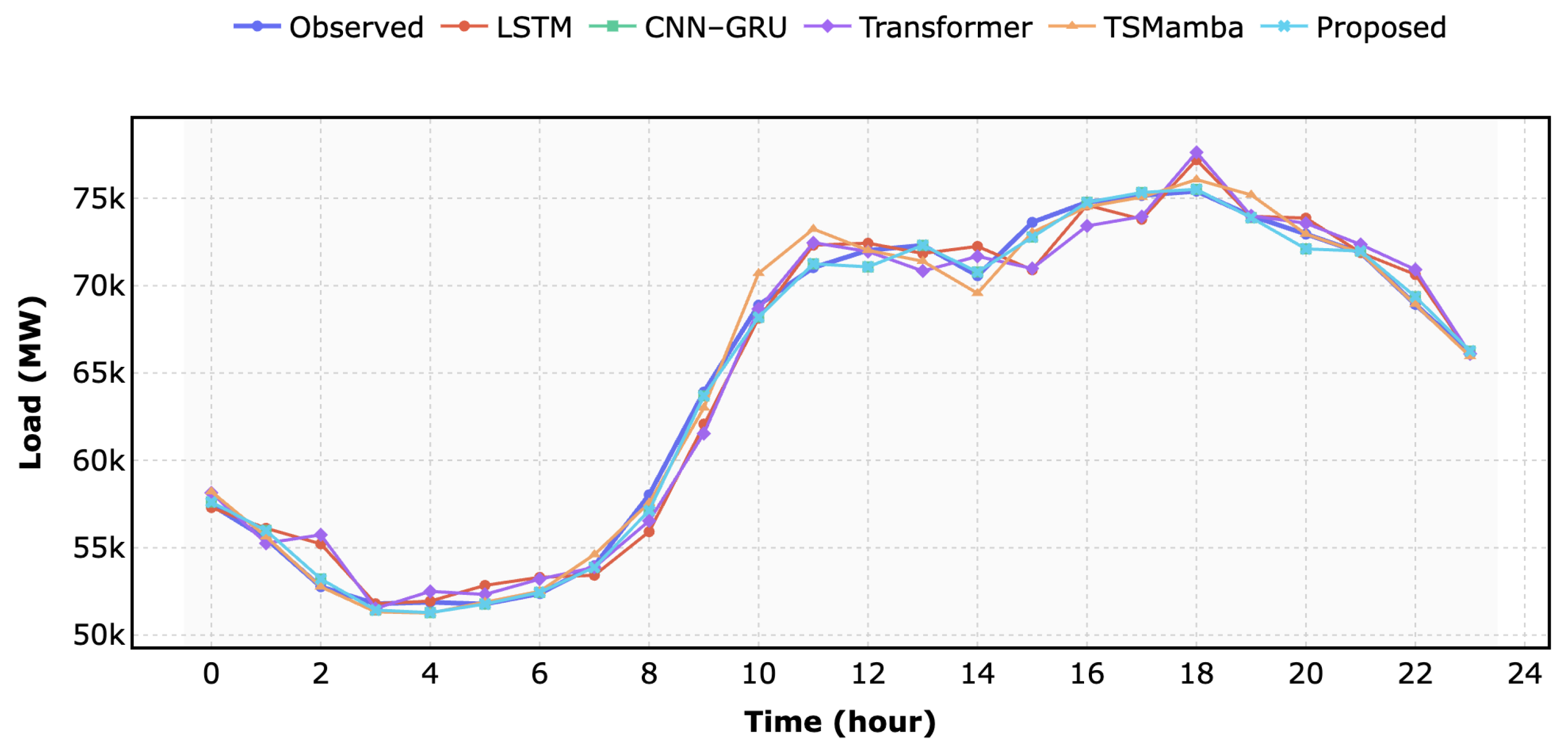
Weekday load profiles are characterized by strong diurnal regularity driven by work–activity cycles with a pronounced morning ramp and evening peak. Figure 6 compares weekdays hourly electrical load with forecasts produced by the models over a 24-h period. As shown in Table 5, all models achieve their lowest errors on weekdays relative to other profiles, reflecting the higher predictability of these patterns. Among the baselines, CNN–GRU outperforms LSTM and Transformer in terms of MAE and WAPE, indicating the benefit of local temporal feature extraction. TSMamba further reduces proportional error compared to attention-based models, suggesting improved handling of longer temporal dependencies. The proposed cluster-conditioned TSMamba achieves the lowest MAE (307.261 MW) and WAPE (0.473%), along with the smallest CVRMSE (0.591%), indicating not only improved point-wise accuracy but also reduced error dispersion relative to the mean load. This improvement highlights the advantage of conditioning state-space dynamics on weekday-specific cluster characteristics, allowing the model to adapt to subtle intra-day structural variations.

4.2.2. Weekend Performance

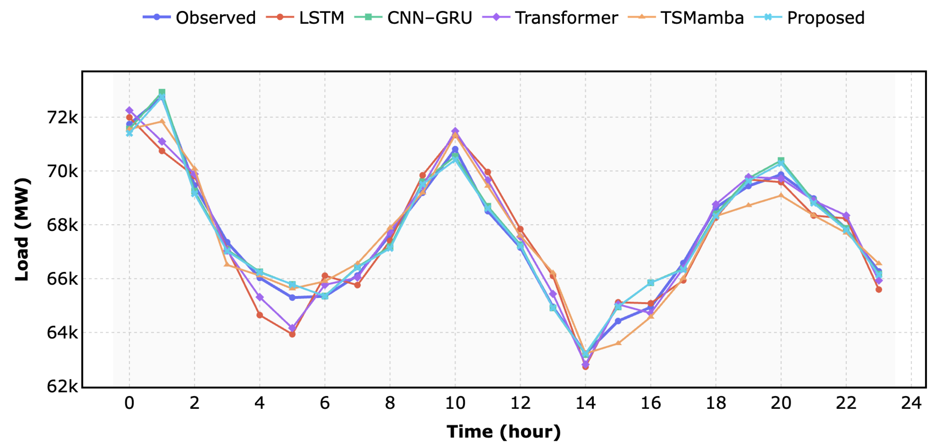
Weekend load profiles represent the most challenging profile characterized by irregular activity schedules with multiple peaks, and increased variability across hours. Figure 7 compares weekend hourly electrical load with forecasts produced by the models over a 24-h period. These shifts pose challenges for models trained primarily on weekday-dominated data. This is reflected in the performance degradation observed for LSTM, Transformer, and TSMamba, all of which exhibit increased MAE and WAPE on weekends. Notably, Transformer and TSMamba show a pronounced rise in CVRMSE, indicating reduced stability under altered demand dynamics. In contrast, the proposed model maintains the lowest errors across all three metrics on weekends, achieving a WAPE of 0.395% and a CVRMSE of 0.501%. This robustness suggests that the cluster-aware formulation effectively captures weekend-specific load profiles and mitigates the impact of distributional shifts between weekday and weekend patterns.

4.2.3. Holiday Performance

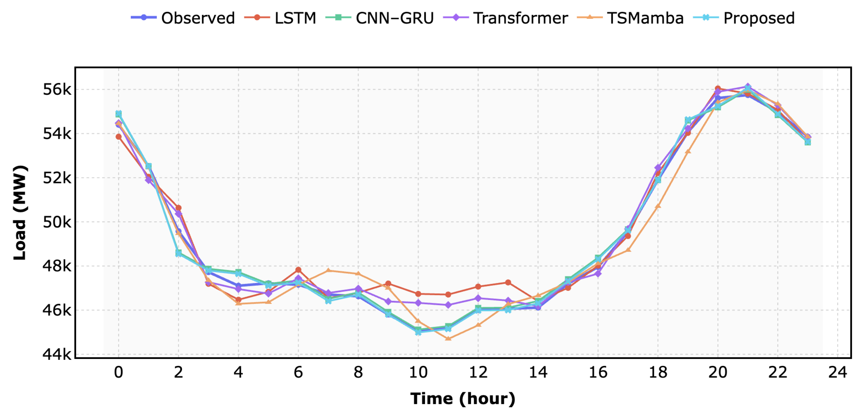
Holiday demand patterns deviate substantially from weekday behavior, exibiting morning peaks and flatter mid-day consumption, characterized by regular activity schedules, suppressed industrial demand, and abrupt transitions before and after the holiday period. Figure 8 shows hourly holiday Load forecasting performance. All models experience their highest errors for holidays, particularly in CVRMSE, reflecting increased volatility relative to the mean load. LSTM exhibits the largest degradation, with a WAPE exceeding 1.1%, underscoring its sensitivity to nonstationary and low-regularity patterns. While CNN–GRU and Transformer offer moderate improvements, their CVRMSE values remain elevated, indicating persistent dispersion in forecast errors. The proposed model again demonstrates superior robustness, achieving the lowest MAE (205.742 MW) and WAPE (0.417%) among all methods. Although CVRMSE increases relative to weekdays, its magnitude remains substantially lower than that of competing models, suggesting more stable performance under highly irregular conditions.

Beyond aggregate performance across predefined temporal categories, an important indicator of practical forecasting reliability is robustness under rapid transitions between load patterns. Such transitions occur frequently at weekday–weekend boundaries and during pre- and post-holiday periods. In particular, holidays occurring on weekdays disrupt regular weekday demand, leading to abrupt shifts in load behavior. To explicitly examine this aspect,

Table 6. Average forecasting error metrics across load pattern clusters.

Model	Cluster 1			Cluster 2			Cluster 3
	MAE (MW)	CVRMSE (%)	WAPE (%)	MAE (MW)	CVRMSE (%)	WAPE (%)	MAE (MW)	CVRMSE (%)	WAPE (%)
Proposed	249.384	0.524	0.413	271.848	0.519	0.419	254.875	0.477	0.377
Improvement (%)	40.6	39.8	40.6	0.5	6.5	0.5	44.2	43.7	44.1
TSMamba [15]	419.665	0.871	0.695	273.145	0.555	0.421	456.342	0.848	0.675
CCNN–GRU [6]	253.610	0.474	0.420	296.502	0.566	0.457	261.636	0.490	0.387
Transformer [10]	423.892	0.864	0.702	275.092	0.536	0.424	469.187	0.887	0.694
LSTM [8]	470.991	0.945	0.780	407.447	0.788	0.628	665.245	1.201	0.984

Note: Percentage improvements are computed relative to the TSMamba baseline as ${\displaystyle \frac{{\mathrm{Metric}}_{\mathrm{TSMamba}}-{\mathrm{Metric}}_{\mathrm{Proposed}}}{{\mathrm{Metric}}_{\mathrm{TSMamba}}}}\times 100$.

reports the average MAE, CVRMSE, and WAPE across three representative load clusters, each capturing a distinct structural profile identified during the clustering stage.

4.2.4. Cluster-Wise Behavior and Transition Sensitivity

Cluster 1 corresponds to relatively regular load patterns with moderate variability, while Clusters 2 and 3 capture increasingly irregular and high-variance profiles associated with transition days and atypical consumption behavior. As expected, all models exhibit increasing error magnitudes when moving from Cluster 1 to Cluster 3, confirming that pattern transitions impose additional forecasting difficulty. However, the rate at which errors grow differs substantially across models.

The LSTM baseline shows pronounced sensitivity to transitions, with MAE increasing from 470.991 MW in Cluster 1 to 665.245 MW in Cluster 3 and a corresponding rise in CVRMSE and WAPE. This behavior reflects the limited capacity of recurrent architectures to rapidly adapt their internal state when confronted with abrupt profile changes. Transformer-based models demonstrate improved stability relative to LSTM but still suffer noticeable degradation in Cluster 3, particularly in WAPE, indicating reduced proportional accuracy during highly irregular periods.

CCNN–GRU exhibits comparatively balanced performance across clusters, with smaller relative increases in MAE and CVRMSE. This suggests that convolutional feature extraction provides some resilience to short-term structural changes. Nevertheless, its performance still deteriorates under the most volatile profile, highlighting the limitations of fixed receptive fields in capturing longer-range transition dynamics.

4.2.5. Effect of State-Space Modeling

TSMamba consistently improves upon attention-based and recurrent baselines across all clusters, particularly in CVRMSE, indicating more stable error behavior relative to the mean load. This stability can be attributed to the continuous-time state-space formulation, which enables smoother adaptation of latent dynamics when transitioning between profiles. However, without explicit conditioning, TSMamba still exhibits non-negligible error growth in Cluster 3, suggesting that shared dynamics alone are insufficient to fully capture heterogeneous transition behavior.

Increasing $\gamma$ gradually shifts learning emphasis toward minority load regimes. As shown in

Table 7. Sensitivity analysis of the cluster-weight exponent $\gamma$.

$\mathit{\gamma }$	Cluster 1 WAPE (%)	Cluster 2 WAPE (%)	Cluster 3 WAPE (%)
0.00	0.697	0.421	0.677
0.25	0.610	0.422	0.600
0.50	0.520	0.421	0.520
0.75	0.445	0.420	0.455
1.00	0.414	0.419	0.378
1.25	0.425	0.419	0.395
1.50	0.455	0.420	0.430
1.75	0.490	0.421	0.465
2.00	0.520	0.422	0.500

, intermediate values progressively reduce error in Clusters 1 and 3 while maintaining stable performance for the dominant Cluster 2. The best overall balance occurs at $\gamma =1$.

4.3. Discussion

The results demonstrate that robustness to load pattern transitions is a critical determinant of forecasting performance. Models relying on a single, globally shared representation exhibit increasing error as load dynamics shift from regular weekday behavior to irregular weekend and holiday profiles. This degradation is particularly evident during transition periods, such as weekday–weekend boundaries and holidays occurring on weekdays, where conventional temporal patterns are disrupted.

By contrast, the proposed cluster-conditioned TSMamba consistently achieves lower and more uniform error across all profiles, confirming the effectiveness of conditioning state dynamics on latent load patterns. Compared to the vanilla TSMamba, the proposed model reduces WAPE by approximately 15% on weekdays (0.559% → 0.473%), 42% on weekends (0.685% → 0.395%), and 39% on holidays (0.683% → 0.417%). Similar improvements are observed in MAE and CVRMSE, indicating that performance gains are systematic rather than metric-specific. These results confirm that cluster-conditioned state modulation effectively mitigates error amplification during rapid profile transitions.

The cluster-level analysis further reinforces this conclusion. While all models perform best under stable weekday-dominated clusters, error increases substantially for clusters associated with irregular or transition-heavy patterns. The proposed model achieves the largest relative gains in these challenging clusters, demonstrating improved alignment between learned state dynamics and profile-specific load behavior. This validates the hypothesis that explicit profile conditioning enables more stable state evolution under non-stationary conditions.

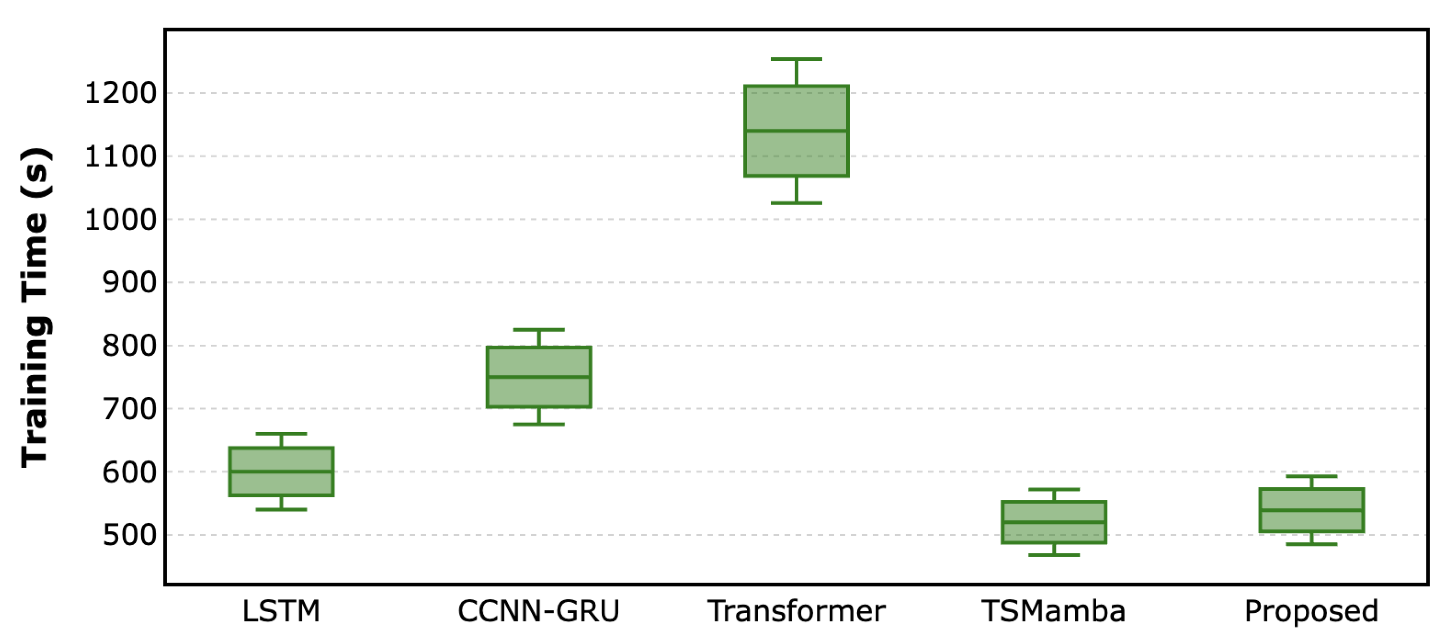
From a computational standpoint, Figure 9 shows that the proposed method exhibits execution times tightly clustered around those of the base TSMamba, with only a marginal overhead in both median and spread. Both models remain substantially faster than Transformer-based architectures, whose execution times are more than twice as large and display higher variability. While LSTM and CCNN–GRU achieve lower absolute runtimes, they do so at the expense of forecasting accuracy and robustness under pattern transitions. This favorable accuracy–efficiency trade-off makes the proposed approach particularly suitable for operational short-term load forecasting, where scalability and robustness under profile shifts are essential.

Inference latency is also critical for operational deployment. On the evaluated hardware platform, generating a single 24-h forecast requires only a few milliseconds, which satisfies real-time operational requirements such as dispatch scheduling and market clearing. This low latency stems from the linear-time sequence processing of state-space architectures like Mamba, which avoid the quadratic complexity of attention-based models, allowing the proposed cluster-conditioned TSMamba to maintain both computational scalability and improved forecasting accuracy.

Overall, the results confirm that cluster-conditioned state-space modeling provides a principled and computationally efficient solution for handling heterogeneous and transition-driven load dynamics, delivering consistent accuracy improvements across diverse operating conditions.

5. Conclusions and Future Work

This paper presents an imbalance-aware TSMamba framework for short-term load forecasting that improves robustness across heterogeneous load patterns while preserving temporal continuity. The proposed method integrates load-shape clustering as causal conditioning covariates within a sequence-continuous SSM and further mitigates pattern imbalance using a cluster-weighted training objective. Empirical results on nationwide KPX hourly demand data [28] show that the proposed cluster-conditioned TSMamba delivers consistent accuracy gains across both dominant and infrequent regimes. Relative to the vanilla TSMamba baseline [15], WAPE is reduced by approximately 15% on weekdays (0.559% → 0.473%), 42% on weekends (0.685% → 0.395%), and 39% on holidays (0.683% → 0.417%), with corresponding reductions in MAE and CVRMSE. Cluster-level evaluation further confirms that the largest relative improvements occur in transition-heavy and irregular regimes, validating the premise that explicit regime conditioning stabilizes latent state evolution and reduces error amplification when demand patterns shift. From an efficiency standpoint, the proposed approach maintains near-linear training complexity with only marginal overhead relative to the base TSMamba, while remaining substantially faster than Transformer-based alternatives, supporting practical deployment under operational latency and scalability constraints.

Future work will focus on three extensions: probabilistic forecasting via distributional or quantile-based objectives to provide calibrated uncertainty under rare and transition regimes, and multi-region forecasting by integrating cluster-conditioned SSMs with spatial representations to capture cross-area dependencies at scale.