Optimal Sizing and Hourly Scheduling of Wind-PV-Battery Systems for Islanded Expressway Service Area Microgrids Under Tiered Electricity Pricing

Abstract

External electricity supplementation for islanded microgrids at expressway service areas is often settled under tiered electricity pricing based on cumulative energy consumption, where marginal prices increase discontinuously once tier thresholds are exceeded. This mechanism reshapes battery dispatch behavior and may alter economically optimal storage sizing. This paper proposes a unified planning—operation optimization framework for wind–PV–battery microgrids that jointly determines the storage capacity and hourly scheduling while enforcing power balance, battery state-of-charge dynamics, and tiered settlement costs. By introducing tier-wise energy allocation variables and tier cap constraints, the nonlinear settlement rule is reformulated into an equivalent piecewise-linear structure, leading to a mixed-integer linear programming (MILP) model that can be solved using standard optimization solvers. A season-weighted annualized case study using four typical seasonal days reveals critical cross-tier dispatch behaviors, where charging–discharging schedules shift near tier boundaries and external electricity purchases are actively suppressed from entering higher-priced tiers. The proposed framework quantifies the premium-avoidance value of storage and provides a practical decision support tool for premium risk-aware sizing and operation of islanded expressway service-area microgrids.

1. Introduction

Against the backdrop of dual-carbon goals and the national strategy to build a strong transportation sector, expressways are evolving from pure transportation corridors into integrated transportation–energy infrastructures [1]. Along corridor nodes such as service areas, toll stations, and tunnel clusters, the large-scale deployment of distributed photovoltaic (PV) and wind generation, coupled with battery energy storage systems (BESSs) and electric vehicle (EV) charging facilities, has emerged as a practical pathway to improve the resilience of the power supply of transportation infrastructure and reduce carbon emissions in the transport sector [2,3]. Meanwhile, the rapid growth of EV penetration leads to pronounced peak–valley characteristics and significant temporal uncertainty in service area demand [4]. Together with the intermittency and volatility of wind and PV generation, these factors exacerbate the spatiotemporal mismatch between supply and demand, posing new challenges to both capacity planning accuracy and operational decision making [5].

A growing body of research has investigated the planning and operation of expressway integrated energy systems and microgrids. In terms of planning and capacity sizing, most studies optimize the installed capacities of wind–PV–storage systems by minimizing life cycle cost or maximizing renewable energy utilization. Carbon trading mechanisms have been incorporated into storage planning for expressway multi-microgrids to quantify the impact of low-carbon constraints [6], while different construction modes and grid connection structures have been examined to evaluate their influence on investment economics [7]. For islanded settings, source–load matching characteristics have been analyzed, highlighting the role of temporal complementarity in reducing storage sizing requirements [8]. Subsequent works further improved engineering realism by incorporating geographical constraints [9], land use limitations [10], and multi-objective trade-offs between economic and environmental criteria [11,12]. However, a common simplification across these planning models is the treatment of external emergency supplementation or grid purchases using linear or fixed tariffs. This assumption is often acceptable in grid-connected systems, yet it can be inadequate for islanded service areas that rely on emergency diesel generators or temporary supply channels, where settlement rules may follow nonlinear mechanisms. As a result, the cost avoidance value of storage may be underestimated, and the resulting sizing decisions can be biased.

On the operational side, energy management strategies aim to cope with renewable and demand uncertainty and achieve economical dispatch. Daily operation optimization for PV–storage–charging systems has been investigated by combining simulation platforms with intelligent optimization algorithms [13], and improved swarm intelligence approaches have been developed for economic dispatch in microgrids with wireless charging [14]. To address uncertainty in wind and PV output and EV charging demand, stochastic programming [15], robust optimization [16], and model predictive control (MPC) [17] have been widely applied to day-ahead and real-time scheduling. Price-based demand response has also been shown to mitigate load fluctuations and reduce operating costs [18]. Nevertheless, most existing operational studies assume that marginal electricity prices are constant or time-of-use prices are exogenously known, and they typically ignore the dependence of the marginal purchase cost on cumulative consumption within a settlement period. This simplification prevents a full characterization of a key strategic role of storage: regulating cumulative external purchases to avoid high-cost regions.

Tiered electricity pricing, also referred to as an inclining block tariff, is a representative nonlinear settlement mechanism used for large industrial customers, emergency power supply, and remote area electricity services [19]. Unlike time-of-use pricing, tiered pricing features stepwise increases in marginal cost triggered by cumulative energy consumption over a settlement horizon; this characteristic has been documented in both residential demand response and industrial energy management contexts [20,21]. Previous studies have shown that nonlinear tariffs can fundamentally reshape storage dispatch strategies [22], and tiered pricing mechanisms can significantly influence aggregated charging costs for EV charging stations [23]. Reviews in the microgrid literature further indicate that linear tariff models may fail to capture the threshold effects induced by nonlinear pricing, potentially leading to suboptimal dispatch decisions [24,25]. However, most existing works focus on grid-connected microgrids or charging stations, implicitly assuming an upstream grid with an unlimited supply capacity [26,27]. This assumption does not hold for islanded expressway service areas, where external supplementation is typically subject to strict power limits. In such systems, limited supplementation capacity, cumulative energy triggering of tier thresholds, and storage energy regulation interact in a strongly coupled manner. The marginal cost jumps at tier boundaries may induce non-traditional behaviors, such as critical cross-tier avoidance [28], which in turn alters the economically optimal storage sizing. Therefore, the conventional decoupled workflow—planning first and operating later—may be insufficient when planning and operation are tightly coupled through tiered settlement constraints [29]. Moreover, systematic quantitative evidence remains limited regarding (1) how tiered pricing risk evolves across seasons and (2) how the external supplementation limit induces threshold effects on overall system economics in islanded expressway scenarios [30].

To further position this study within the existing literature,

Table 1. Comparison of representative studies on expressway or islanded wind–PV–storage system optimization.

Reference	Scenario	Method	Pricing	Storage Sizing	Main Limitation
[6]	Expressway multi-microgrid	Planning optimization	Carbon trading	Yes	No tiered settlement mechanism
[7]	Expressway microgrid	Capacity configuration	Linear tariff	Yes	No endogenous settlement modeling
[8]	Islanded service area	Source–load matching	Fixed tariff	Yes	No hourly coordinated scheduling
[13]	PV–storage–charging station	Heuristic scheduling	Time of use	Limited	No cumulative tier-triggering effect
[31]	Multi-energy-integrated highway service center	Economic scheduling	Conventional tariff	No	Lack of joint sizing–operation optimization under tiered settlement
[32]	Off-grid highway service area self-contained energy system	Stochastic–robust planning	Conventional electricity cost	Yes	No explicit modeling of cumulative tiered settlement
This work	Islanded expressway service area	MILP	Tiered settlement	Yes	Endogenous planning–operation coupling under cumulative tiered pricing mechanism

summarizes representative studies on expressway or islanded wind–PV–storage systems in terms of the application scenario, optimization method, pricing mechanism, storage sizing treatment, and main limitations. The comparison shows that although prior studies have addressed planning, configuration, and scheduling problems, most of them relied on linear, fixed, or time-of-use tariffs and did not explicitly capture the cumulative tier-triggering effect of external electricity settlement. Moreover, the endogenous coupling between storage sizing and hourly operation under tiered settlement remains insufficiently explored for islanded expressway service area microgrids.

As summarized in Table 1, existing studies rarely develop a unified optimization framework that simultaneously considers storage sizing, hourly scheduling, and cumulative tiered settlement for islanded expressway service area microgrids. Most prior work either assumed linear or fixed electricity pricing or focused on dispatch without explicitly characterizing the premium risk mechanism induced by cumulative external electricity purchases:

(1)

A tiered settlement-coupled modeling framework is developed, reformulating the economic mechanism of cumulative energy tier crossing and marginal price jumps into an optimization-embedded piecewise cost structure so that premium risk becomes an endogenous outcome rather than an ex post accounting term.

(2)

A mixed-integer linear programming (MILP) formulation is derived that can be solved directly by off-the-shelf solvers. By introducing tier-wise energy allocation variables and tier cap constraints, the tiered pricing rule is transformed into an equivalent piecewise-linear representation, enabling integrated capacity sizing, dispatch decisions, and tiered settlement modeling in a single optimization model.

(3)

Season-weighted annualized case studies with scenario perturbations reveal critical cross-tier dispatch behaviors under tiered settlement, quantify the additional premium avoidance value of storage, and identify time-of-day sources of tier triggering, providing a practical and interpretable decision tool for wind–PV–storage planning and operation at expressway service areas.

The remainder of this paper is organized as follows. Section 2 describes the problem setting and islanded operation scenario. Section 3 presents aggregated models for sources, loads, storage, and external supplementation. Section 4 formulates the tiered settlement-embedded MILP model and the solution procedure. Section 5 reports the case studies and scenario analyses. Section 6 concludes the paper and outlines future work.

2. Problem Statement

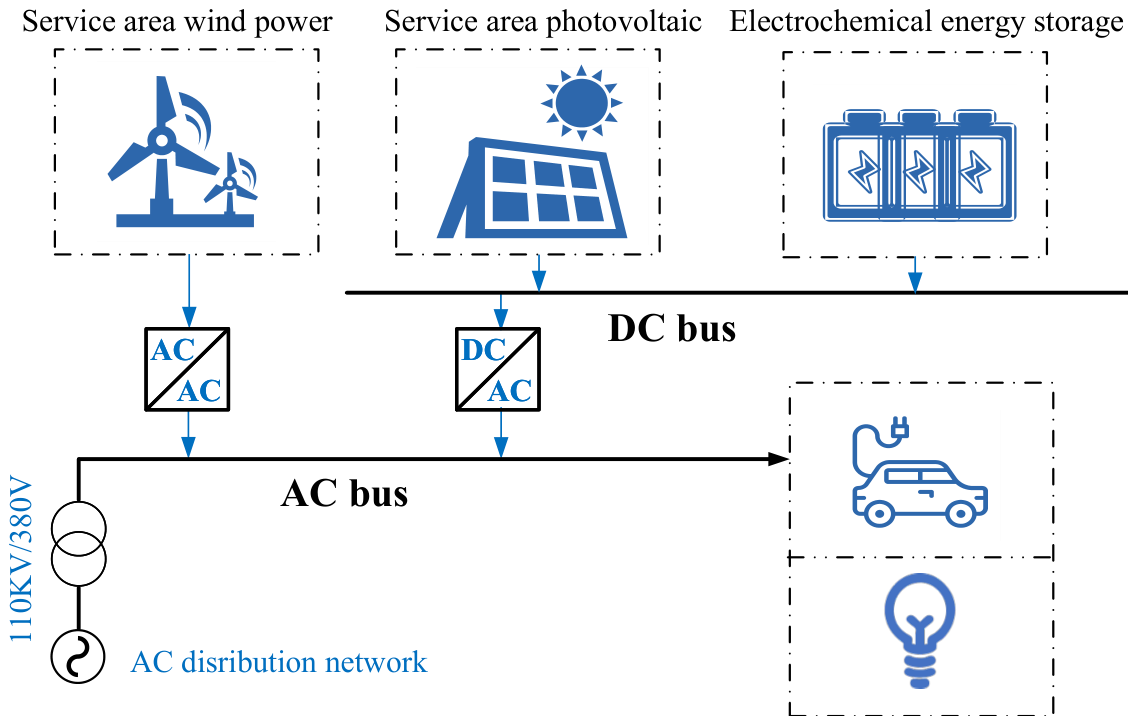
This paper considers an islanded expressway service area integrated energy system, as schematically illustrated in Figure 1. The system includes wind generation, photovoltaic generation, a battery energy storage system, and corridor loads, coupled through AC/DC converters. Under islanded operation, local renewables and storage serve as the primary energy sources. When renewable output is insufficient, storage is constrained, or the continuity of critical loads must be guaranteed, the system can draw electricity through an external supplementation channel, such as emergency diesel generation, mobile storage vehicles, or temporary power connections. For unified modeling, this channel is represented as an adjustable external power source, with its settlement cost governed by tiered pricing.

The operating horizon is modeled at an hourly resolution with daily settlement. Wind and PV power profiles are provided by forecast models driven by meteorological data, while service area demand is represented as the aggregation of building and facility loads, EV charging loads, and critical corridor loads such as toll stations and long tunnels. These renewable and demand trajectories are treated as exogenous inputs for coordinated sizing and scheduling.

Different from linear pricing, the external supplementation cost follows a tiered settlement mechanism. Within each settlement day, the cumulative supplemented energy is billed at increasing unit prices across energy blocks. Consequently, the external cost is not solely determined by the instantaneous power or total daily energy in a linear manner but depends on the tier membership of cumulative energy. Under this mechanism, the economic value of storage extends beyond conventional peak shaving and valley filling. Storage can also reduce cumulative external energy and delay or avoid entering high-price tiers, thereby generating quantifiable premium avoidance benefits. This cumulative energy tier crossing, marginal price jumping, and strategy switching mechanism constitutes the key driver of the proposed integrated planning–operation optimization.

Accordingly, the problem is formulated as the joint decision of storage sizing and hourly operating schedules to minimize the annualized total cost, including annualized investment and operation and maintenance costs, as well as the daily tiered settlement cost of external supplementation. In addition, the model outputs tier-wise energy allocations for each settlement day, enabling explicit interpretation of high-tier triggering sources and premium risk avoidance mechanisms. Scenario perturbations, such as renewable deviations, demand changes, and tariff parameter variations, are further used to evaluate robustness, sensitivity, and interpretability under practical engineering conditions.

3. Modeling of the Expressway Microgrid

An aggregated equivalent model is adopted for the service area energy system, where a single-node power balance captures the coupling among sources, loads, storage, and external supplementation.

3.1. Source-Side Modeling of Renewables

3.1.1. Wind Resource and Wind Power Output

Wind power output is derived from the measured wind speed using a typical turbine power curve [33]. Considering the surrounding terrain, clearance and height constraints along the roadway, as well as operational safety requirements, a low wind speed, small-to-medium wind turbine was selected. The power–speed relationship of the wind turbine is expressed as follows:

$$P_{w,t}\left(v_t\right)=\left\{\begin{array}{cc}0,\hfill & v_t\le v_{ci}\mathrm{or}{v}_t\ge v_{co},\hfill \\ P_w^R{\displaystyle \frac{v_t-v_{ci}}{v_r-v_{ci}}},\hfill & v_{ci}<v_t\le v_r,\hfill \\ P_w^R,\hfill & v_r<v_t<v_{co}.\hfill \end{array}\right.$$

(1)

where $v_t$ denotes the wind speed at hour t; $v_{ci}$, $v_r$, and $v_{co}$ are the cut-in, rated, and cut-out wind speeds, respectively; and $P_w^R$ is the rated power of a single wind turbine.

To enable scenario perturbations via scalable mappings, a per-unit wind availability coefficient ${\tilde{p}}_{d,t}^{\mathrm{W}}$ is defined to represent the available wind output per-unit installed capacity at hour t of a typical day d. Thus, the aggregated wind output is

$$P_{w,d,t}=P_w^{\mathrm{cap}}{\tilde{p}}_{d,t}^{\mathrm{W}},$$

(2)

where $P_w^{\mathrm{cap}}$ is the total installed wind capacity along the expressway corridor.

Based on an annual 8760-h wind speed series, the annual wind energy production and the wind capacity factor can be obtained as follows:

$$E_w=\sum _{t=1}^T{P}_{w,t}\Delta t,C{F}_w={\displaystyle \frac{E_w}{P_w^{\mathrm{cap}}{T}_{\mathrm{year}}}}$$

(3)

where $T_{\mathrm{year}}$ denotes the annual duration.

3.1.2. Solar Resource and PV Power Output

For PV generation, a hierarchical modeling approach from resource to component and then to system is adopted [34]. Horizontal irradiance is converted to the plane-of-array irradiance $G_r\left(t\right)$ by accounting for module tilt, azimuth, and shading effects. The PV output at hour t is modeled as

$$P_{pv,t}=P_{pv}^{\mathrm{cap}}{\displaystyle \frac{G_r\left(t\right)}{G_{\mathrm{STC}}}}\left[1+k_p\left(T_{\mathrm{cell}}\left(t\right)-T_{\mathrm{STC}}\right)\right]{\eta }_{\mathrm{inv}},$$

(4)

where $P_{pv}^{\mathrm{cap}}$ is the installed PV capacity; $G_{\mathrm{STC}}$ and $T_{\mathrm{STC}}$ are the irradiance and temperature under standard test conditions (STCs), respectively; $k_p$ is the temperature coefficient; $T_{\mathrm{cell}}\left(t\right)$ is the cell temperature; and ${\eta }_{\mathrm{inv}}$ is the combined efficiency of the inverter and PV system.

Similarly, a PV per unit coefficient ${\tilde{p}}_{d,t}^{\mathrm{PV}}$ is defined. The PV power output can be expressed as

$$P_{pv,d,t}=P_{pv}^{\mathrm{cap}}{\tilde{p}}_{d,t}^{\mathrm{PV}}$$

(5)

The corresponding annual PV energy and capacity factor are

$$E_{pv}=\sum _{t=1}^T{P}_{pv,t}\Delta t,C{F}_{pv}={\displaystyle \frac{E_{pv}}{P_{pv}^{\mathrm{cap}}{T}_{\mathrm{year}}}}.$$

(6)

3.1.3. Wind–PV Complementarity and Power Fluctuation Modeling

The total renewable output is

$$P_{ren,d,t}=P_{w,d,t}+P_{pv,d,t}.$$

(7)

Complementarity is quantified using the correlation coefficient between wind and PV outputs:

$${\rho }_{w,pv}={\displaystyle \frac{{\sum }_t\left(P_{w,t}^{\mathrm{tot}}-{\overline{P}}_w\right)\left(P_{pv,t}^{\mathrm{tot}}-{\overline{P}}_{pv}\right)}{\sqrt{{\sum }_t{\left(P_{w,t}^{\mathrm{tot}}-{\overline{P}}_w\right)}^2}\sqrt{{\sum }_t{\left(P_{pv,t}^{\mathrm{tot}}-{\overline{P}}_{pv}\right)}^2}}}$$

(8)

Here, ${\overline{P}}_w$ and ${\overline{P}}_{pv}$ are the mean values of the corresponding power series. A more negative correlation indicates stronger complementarity, which can reduce storage requirements. Scenario perturbations are generated by scaling the per-unit renewable profiles.

3.2. Modeling of the Load Side

It should be noted that the present study focuses on capacity planning and hourly energy scheduling at the active power layer. Therefore, the load is modeled in an aggregated active power form to capture temporal demand variations, rather than static or dynamic characteristics associated with the voltage and frequency. Such load behaviors are important for transient and small-signal stability studies, but they are beyond the scope of the present MILP-based economic optimization framework.

The proposed framework is intended for upper-layer planning and economic dispatch, whereas voltage and frequency dynamics belong to lower-layer operation and control. In practical applications, these dynamic characteristics can be further evaluated in a subsequent validation stage using detailed power–flow or electromagnetic simulation models.

The service area load consists of three components: building and auxiliary loads, aggregated electric-vehicle (EV) charging load, and corridor-critical loads (e.g., toll stations and long tunnels). The total load is

$$P_{load,d,t}=P_{srv,d,t}+P_{EV,d,t}+P_{\mathit{tol-tun},d,t}$$

(9)

3.2.1. Service Area Building Loads

Building loads include HVAC, lighting, hot water, ICT, and commercial facilities, exhibiting both daily periodicity and seasonal variation. A compact parametric form is adopted:

$$P_{srv,d,t}=P_{\mathrm{base}}^{\mathrm{B}}\left({\alpha }_d\left(h_t\right)+{\alpha }_s\left(d_t\right)+{\alpha }_T\left(T_t\right)\right)$$

(10)

where $P_{\mathrm{base}}^{\mathrm{B}}$ is the baseline building load; $h_t$, $d_t$, and $T_t$ are the hour index, season index, and outdoor temperature, respectively; and ${\alpha }_d(·)$, ${\alpha }_s(·)$, and ${\alpha }_T(·)$ are fitted factors representing diurnal, seasonal, and temperature effects, respectively.

3.2.2. EV Charging Load Modeling

EV charging demand is the most uncertain component, being affected by traffic flow, EV penetration, the arrival time distribution, holiday patterns, and weather. A traffic–behavior–charging modeling pipeline is adopted [35]. First, traffic data are used to estimate the hourly arrival rate. Then, the SOC distribution and user preferences are incorporated to model charging decisions. Finally, charger types and queuing effects are considered to generate the hourly charging profile.

A simplified aggregated representation is used:

$$P_{EV,d,t}={\eta }_{\mathrm{chg}}{N}_{EV,d,t}{E}_{\mathrm{per}}$$

(11)

where $N_{EV,d,t}$ is the number of arriving vehicles requesting charging at hour t of a typical day d, ${\eta }_{\mathrm{chg}}$ is the charging efficiency, and $E_{\mathrm{per}}$ is the average charging energy per vehicle.

In practice, charging demand often exhibits pronounced morning and evening peaks and holiday-driven clustering. In scenario studies, the EV charging profile is scaled to represent traffic growth or holiday surges.

3.2.3. Toll Station and Long-Tunnel Load Modeling

These corridor-critical loads are relatively stable and are modeled as the baseline plus auxiliary components:

$$P_{\mathit{tol-tun},d,t}=P_{tol,d,t}+P_{tun,d,t},$$

(12)

$$P_{tol,d,t}=P_{tol,\mathrm{base}}+P_{tol,\mathrm{aux}},$$

(13)

$$P_{tun,d,t}=P_{tun,\mathrm{base}}+P_{tun,\mathrm{aux}},$$

(14)

where $P_{tol,\mathrm{base}}$ and $P_{tun,\mathrm{base}}$ denote the baseline power of toll stations and tunnels, respectively, and $P_{tol,\mathrm{aux}}$ and $P_{tun,\mathrm{aux}}$ represent auxiliary loads such as monitoring, communication, and other supporting equipment. Although tunnel demand may depend on traffic volume and environmental conditions, its fluctuation is typically limited; therefore, it is treated as a critical load with priority in source–load–storage matching and capacity planning.

Demand response is not explicitly modeled in the present study. The load profiles are treated as exogenous inputs, and the current framework focuses on supply-side coordination and storage-based flexibility. Nevertheless, demand response can be incorporated in future work by introducing shiftable or interruptible load variables and corresponding user-side operational constraints, thereby further enhancing the flexibility of the islanded service area energy system.

3.3. Modeling of Battery Energy Storage System

The battery energy storage system is modeled with its energy-state dynamics and power constraints at an hourly resolution [36]. Let $E_{\mathrm{cap}}^{\mathrm{bess}}$ and $P_{\mathrm{cap}}^{\mathrm{bess}}$ denote the energy capacity and power rating, respectively. With the charging and discharging power $P_{d,t}^{\mathrm{ch}}$ and $P_{d,t}^{\mathrm{dis}}$, respectively, and round-trip efficiency ${\eta }_{\mathrm{bess}}$, the State-of-charge (SOC) dynamics are

$${\mathrm{SOC}}_{d,t+1}={\mathrm{SOC}}_{d,t}+{\displaystyle \frac{{\eta }_{\mathrm{bess}}{P}_{d,t}^{\mathrm{ch}}-\left(P_{d,t}^{\mathrm{dis}}/{\eta }_{\mathrm{bess}}\right)}{E_{\mathrm{cap}}^{\mathrm{bess}}}}\Delta t$$

(15)

SOC bounds and charge and discharge power limits are enforced. To avoid simultaneous charging and discharging, binary variables are introduced to maintain an MILP structure and improve interpretability. This storage model provides the state-variable basis for optimizing strategies that suppress the daily cumulative external energy from crossing tier thresholds.

3.4. Modeling of External Power Supplementation and Tiered Settlement

It should be emphasized that the external supplementation channel in this study is modeled in an abstract and unified manner. The adopted daily tiered pricing structure does not aim to represent one specific physical supply mode only but rather capture a generalized cumulative procurement cost mechanism in which the marginal supplementation cost increases with the total externally supplied energy within the settlement horizon. This abstraction is intended to reflect practical situations where emergency or auxiliary electricity procurement becomes progressively more expensive as reliance on external support increases.

Under islanded operation, when renewables and storage cannot satisfy demand, the system uses an external supplementation channel (e.g., mobile generators, temporary grid connection, or energy trucks). Let $P_{d,t}^{\mathrm{ex}}$ denote the external supply power. Considering a daily settlement based on tiered pricing, the scheduling horizon is divided into a set of days $\mathcal{D}$, where $d\in \mathcal{D}$ denotes the dth day and each day is discretized into an hourly set $\mathcal{T}$ with a time step $\Delta t$ (here, $\Delta t=1\mathrm{h}$). The cumulative external energy on day d is defined as follows:

$$E_d^{\mathrm{ex}}=\sum _{t\in \mathcal{T}}{P}_{d,t}^{\mathrm{ex}}\Delta t$$

(16)

A tiered pricing mechanism with K tiers is considered, with strictly increasing unit prices ${\pi }_1<\cdots <{\pi }_K$. Tier caps ${\overline{E}}_k$ are specified for the first $K-1$ tiers (the last tier is unbounded). We introduce tier-wise energy variables $e_{d,k}\ge 0$, representing the portion of day d’s cumulative energy allocated to tier k. The cumulative energy can then be decomposed as follows:

$$\sum _{k=1}^K{e}_{d,k}=E_d^{\mathrm{ex}},0\le e_{d,k}\le {\overline{E}}_k,k=1,\dots ,K-1$$

(17)

The daily tiered settlement cost is

$$C_d^{\mathrm{ex}}=\sum _{k=1}^K{\pi }_k{e}_{d,k}$$

(18)

This modeling approach converts the stepwise marginal cost structure of tiered pricing into linear constraints, enabling the optimizer to endogenously determine the tier allocation of purchased energy and guide storage dispatch toward avoiding high price tiers.

4. MILP Formulation for Joint Sizing and Coordinated Operation Under Tiered Pricing

Based on the source–load–storage–external models established above, this section develops a joint planning–operation MILP for an expressway service area wind–PV–BESS system on an hourly time grid. The battery is treated as an energy buffer to maximize renewable utilization while minimizing the cost of external electricity supplementation under tiered settlement. Within each hour, any imbalance between renewable generation and demand is first regulated via battery charging and discharging; external supplementation is used only when local renewables and storage cannot satisfy demand. Since external settlement is determined by the accumulated daily purchased energy, the battery provides two types of value: conventional peak shaving or valley filling and explicit cross-tier premium avoidance.

4.1. Decision Variables and Deterministic Modeling

Decision variables are organized into three layers: planning, operation, and settlement.

4.1.1. Planning-Layer Variables (Capacity Decisions)

$$\mathbf{x}={\left[P_{pv}^{\mathrm{cap}},P_w^{\mathrm{cap}},E_{\mathrm{bess}}^{\mathrm{cap}},P_{\mathrm{bess}}^{\mathrm{cap}},P_{\mathrm{ex}}^{max}\right]}^{\mathsf{T}}$$

(19)

where $P_{pv}^{\mathrm{cap}}$ and $P_w^{\mathrm{cap}}$ denote the installed PV and wind capacities, respectively; $E_{\mathrm{bess}}^{\mathrm{cap}}$ and $P_{\mathrm{bess}}^{\mathrm{cap}}$ are the battery energy and power ratings, respectively; and $P_{\mathrm{ex}}^{max}$ is the maximum admissible exchange power of the external supplementation channel.

4.1.2. Operation-Layer Variables (Hourly Operating States and Actions)

$$\mathbf{y}={\left\{P_{d,t}^{\mathrm{ch}},P_{d,t}^{\mathrm{dis}},{\mathrm{SOC}}_{d,t},P_{d,t}^{\mathrm{ex}},U_{\mathrm{bess},d,t},U_{\mathrm{ex},d,t}\right\}}_{t\in \mathcal{T}}$$

(20)

where $U_{\mathrm{bess},d,t}\in \{0,1\}$ is the binary variable enforcing mutually exclusive charging and discharging (one for charging and zero for discharging) and $U_{\mathrm{ex},d,t}\in \{0,1\}$ indicates the external transaction status (one for purchasing and zero for selling, if selling is allowed in the setting).

4.1.3. Settlement-Layer Variables (Tier Allocation)

$$\mathbf{e}={\left\{e_{d,1},e_{d,2},\dots ,e_{d,K}\right\}}_{d\in \mathcal{D}}$$

(21)

where $e_{d,k}$ denotes the portion of day d’s purchased energy allocated to tier k.

4.2. Objective Function

The objective is to minimize the annualized total cost, comprising the (1) annualized investment cost, (2) operation and maintenance (O&M) cost, and (3) tiered settlement cost of external supplementation. No additional redundant terms are introduced.

4.2.1. Annualized Investment Cost

Given a planning horizon of Y years and a discount rate r, the capital recovery factor (CRF) is

$$\mathrm{CRF}={\displaystyle \frac{r{(1+r)}^Y}{{(1+r)}^Y-1}}$$

(22)

Let $C_{\mathrm{inv}}^{\mathrm{W}}$, $C_{\mathrm{inv}}^{\mathrm{PV}}$, and $C_E^{\mathrm{ES}}$ denote the unit investment costs of wind, PV, and storage, respectively. The annualized investment cost is then

$$C_{\mathrm{cap}}\left(\mathbf{x}\right)=\mathrm{CRF}\left(C_{\mathrm{inv}}^{\mathrm{W}}{P}_w^{\mathrm{cap}}+C_{\mathrm{inv}}^{\mathrm{PV}}{P}_{pv}^{\mathrm{cap}}+C_E^{\mathrm{ES}}{E}_{\mathrm{bess}}^{\mathrm{cap}}\right)$$

(23)

4.2.2. Operation and Maintenance Cost

O&M is modelled as a fixed proportion of investment plus device-dependent operational maintenance:

$$\begin{array}{cc}\hfill C_{\mathrm{OM}}\left(\mathbf{x}\right)=& \gamma \left(C_{\mathrm{inv}}^{\mathrm{W}}{P}_w^{\mathrm{cap}}+C_{\mathrm{inv}}^{\mathrm{PV}}{P}_{pv}^{\mathrm{cap}}+C_E^{\mathrm{ES}}{E}_{\mathrm{bess}}^{\mathrm{cap}}\right)\hfill \\ \hfill & +\sum _{d\in \mathcal{D}}{\omega }_d\left[\sum _{t\in \mathcal{T}}\left(c_{\mathrm{bess}}^{\mathrm{om}}\left(P_{d,t}^{\mathrm{ch}}+P_{d,t}^{\mathrm{dis}}\right)+c_{\mathrm{ex}}^{\mathrm{om}}{P}_{d,t}^{\mathrm{ex}}\right)\Delta t\right]\hfill \end{array}$$

(24)

where $\gamma$ is the O&M ratio, $c_{\mathrm{bess}}^{\mathrm{om}}$ is the unit O&M cost associated with storage operation, $c_{\mathrm{ex}}^{\mathrm{om}}$ is the unit O&M cost for external supplementation, and ${\omega }_d$ is the annual weight of a typical day d.

4.2.3. Tiered Electricity Procurement Cost

The daily tiered procurement cost $C_d^{\mathrm{ex}}$ is computed with Equation (18) and annualized using the typical-day weights ${\omega }_d$.

4.2.4. Total Objective

Finally, the annualized total cost is

$$\underset{\mathbf{x},\mathbf{y},\mathbf{e}}{min}{C}_{\mathrm{total}}=C_{\mathrm{cap}}\left(\mathbf{x}\right)+C_{\mathrm{OM}}\left(\mathbf{x}\right)+\sum _{d\in \mathcal{D}}{\omega }_d{C}_d^{\mathrm{ex}}$$

(25)

4.3. Constraints

The constraints of the optimization model are organized into several categories, including power balance, renewable generation limits, storage operation constraints, external supply limits, and tiered pricing constraints.

4.3.1. Power Balance Constraints

For each typical day $d\in \mathcal{D}$ and hour $t\in \mathcal{T}$, the active power balance is

$$P_{ren,d,t}+P_{d,t}^{\mathrm{ex}}+P_{d,t}^{\mathrm{dis}}=P_{load,d,t}+P_{d,t}^{\mathrm{ch}}$$

(26)

For tractability, the present study adopts a single-node aggregated power-balance model and does not explicitly model feeder-level active power losses. Such losses are assumed to be either embedded in the aggregated demand data or relatively small compared with the dominant external electricity procurement cost over the studied planning horizon. If needed, active power losses can be incorporated in future work through linearized loss approximations or network-constrained power flow formulations.

4.3.2. Renewable Capacity and Output Constraints

Renewable outputs are bounded by installed capacities and per-unit availability coefficients:

$$0\le P_{w,d,t}\le P_w^{\mathrm{cap}}{\tilde{p}}_{d,t}^{\mathrm{W}},0\le P_{pv,d,t}\le P_{pv}^{\mathrm{cap}}{\tilde{p}}_{d,t}^{\mathrm{PV}}$$

(27)

The installed capacities are limited by engineering bounds:

$$P_w^{min}\le P_w^{\mathrm{cap}}\le P_w^{max},P_{pv}^{min}\le P_{pv}^{\mathrm{cap}}\le P_{pv}^{max}$$

(28)

It is noted that the optimal PV and wind capacities reported in the case study reach their prescribed upper bounds. This does not mean that these capacities are fixed exogenously in the optimization. Rather, it indicates that under the current economic parameters and renewable resource assumptions, the optimizer prefers to install renewable generation up to the admissible engineering limits. These upper bounds reflect the practical site and installation constraints of the considered service area application.

4.3.3. EV Charging Station Capacity Constraint

To guarantee EV charging service capability, the charging station capacity should cover the predicted peak charging power with a reserve margin and is also limited by site and interconnection conditions:

$$k_{\mathrm{EV}}{P}_{\mathrm{EV}}^{max}\le P_{\mathrm{EV}}^{\mathrm{M}}$$

(29)

where $P_{\mathrm{EV}}^{max}$ is the maximum predicted EV charging power among typical days, $k_{\mathrm{EV}}$ is the reserve margin, and $P_{\mathrm{EV}}^{\mathrm{M}}$ is the maximum feasible construction capacity.

4.3.4. Battery Energy Storage Constraints

The SOC dynamics follow Equation (15) and are subject to the bounds

$${\mathrm{SOC}}_{min}\le {\mathrm{SOC}}_{d,t}\le {\mathrm{SOC}}_{max}$$

(30)

with charge and discharge power limits and mutual exclusivity:

$$0\le P_{d,t}^{\mathrm{ch}}\le U_{\mathrm{bess},d,t}{P}_{\mathrm{bess}}^{\mathrm{cap}},0\le P_{d,t}^{\mathrm{dis}}\le (1-U_{\mathrm{bess},d,t})P_{\mathrm{bess}}^{\mathrm{cap}}$$

(31)

Cyclic consistency over a typical day is enforced to facilitate repeated daily scheduling:

$$\sum _{t\in \mathcal{T}}\left({\eta }_{\mathrm{bess}}{P}_{d,t}^{\mathrm{ch}}-{\displaystyle \frac{P_{d,t}^{\mathrm{dis}}}{{\eta }_{\mathrm{bess}}}}\right)\Delta t=0$$

(32)

4.3.5. External Supply Power Constraints

Under islanded operation, an external supply is used for supplementation and emergency support. The hourly external power is nonnegative and bounded by the channel limit:

$$0\le P_{d,t}^{\mathrm{ex}}\le P_{\mathrm{ex}}^{max}$$

(33)

The current framework does not impose an explicit active-power reserve requirement as an independent operational constraint. Instead, system flexibility is represented through the installed renewable capacity, the battery power and energy ratings, and the admissible external supplementation limit. In this sense, the storage system and the external channel jointly provide a certain degree of upward operational flexibility. The explicit modeling of reserve requirements will be considered in future work by introducing reserve-margin constraints at the hourly level.

4.3.6. Tiered Pricing Constraints

The tiered settlement mechanism is embedded linearly with Equations (16)–(18). Specifically, the daily cumulative purchased energy $E_d^{\mathrm{ex}}$ is computed from hourly $P_{d,t}^{\mathrm{ex}}$; the tier allocation variables $e_{d,k}$ decompose $E_d^{\mathrm{ex}}$ across tiers under tier cap constraints; and the daily tiered cost $C_d^{\mathrm{ex}}$ is evaluated using Equation (18) and included in Equation (25). This reformulation converts the nonlinear tier-crossing premium effect into a linear decision structure compatible with standard MILP solvers, enabling storage scheduling to explicitly suppress cumulative external energy from entering high price tiers.

4.3.7. Overall Wind–PV–Storage Coordinated Optimization Model

For clarity of presentation, the decision variables are grouped into three categories: planning variables, operational variables, and settlement variables. All variables used in the optimization model are explicitly defined before formulation of the objective function and constraints.

The complete joint sizing-and-scheduling optimization is summarized as follows:

$$\begin{array}{cc}\hfill \underset{\mathbf{x},\mathbf{y},\mathbf{e}}{min}& C_{\mathrm{cap}}\left(\mathbf{x}\right)+C_{\mathrm{OM}}\left(\mathbf{x}\right)+\sum _{d\in \mathcal{D}}{\omega }_d{C}_d^{\mathrm{ex}}\hfill \\ \hfill \mathrm{s.t.}& \left(26\right)–\left(33\right),\left(16\right)–\left(18\right)\hfill \end{array}$$

(34)

The key distinction from conventional wind–PV–storage optimization is that the tiered tariff is modelled endogenously rather than calculated post hoc. By introducing tier-wise energy allocation variables, the nonlinear marginal price jump induced by cumulative purchased energy is transformed into an equivalent linear structure, allowing the economic value of storage to be quantified explicitly not only via time shifting for peak shaving but also via premium avoidance by preventing cumulative external energy from entering high price tiers.

4.4. Method Solution and Implementation

4.4.1. Solving the Deterministic Baseline Model

The proposed joint planning–operation model is a standard mixed-integer linear programming (MILP) without nonlinear terms and can be solved directly using commercial or open-source MILP solvers. The key linear modelling treatments are (1) enforcing mutually exclusive charging and discharging via binary variables (thus avoiding bilinear products) and (2) reformulating tiered settlement into an equivalent piecewise-linear representation using tier-wise energy allocation variables and tier cap constraints without any if–else logic. All cost components are linear, ensuring global optimality within the MILP framework.

Unlike heuristic algorithms such as particle swarm optimization, ant colony optimization, and simulated annealing, the proposed model is formulated as a standard MILP problem after reformulating the cumulative tiered settlement mechanism into an equivalent linear structure. Therefore, it can be solved directly by off-the-shelf MILP solvers with deterministic convergence and clear optimality guarantees. In contrast, heuristic methods are generally more suitable for nonlinear or black box optimization problems and do not guarantee global optimality. For this reason, heuristic solution procedures are not adopted in the present study. Nevertheless, they may be useful in future extensions involving stronger nonlinearities, nonconvex degradation models, or larger-scale coordinated systems.

4.4.2. Standard Solving Procedure

Based on the unified MILP formulation in Equation (34), the deterministic baseline solution procedure consists of six steps: data preprocessing, variable construction, objective assembly, constraint assembly, optimization solving, and post-processing with performance evaluation. The detailed procedure is summarized in Algorithm 1.

4.5. Solution Framework

The overall solution procedure of the proposed joint sizing and operation optimization framework is illustrated in Figure 2. The framework integrates renewable generation modeling, load representation, MILP formulation, and solver-based optimization into a unified analytical pipeline. It explicitly reflects the interaction between data input, model construction, optimization solving, and economic analysis.

Algorithm 1 Deterministic baseline MILP solving procedure

Input: settlement day set $\mathcal{D}$ and hourly index set $\mathcal{T}$; time step $\Delta t$; wind and PV per-unit profiles ${\tilde{p}}_{d,t}^{\mathrm{W}}$ and ${\tilde{p}}_{d,t}^{\mathrm{PV}}$; load profiles $P_{\mathrm{load},d,t}$; device parameters (e.g., ${\eta }_{\mathrm{bess}}$); capacity bounds (Equation (28)); external supply limit (Equation (33)); tiered tariff parameters including number of tiers K, tier prices $\left\{{\pi }_k\right\}$, and tier caps ${\left\{{\overline{E}}_k\right\}}_{k=1}^{K-1}$; annualization factor $\mathrm{CRF}$ and O&M coefficients in Equations (23) and (24). Output: optimal planning capacities ${\mathbf{x}}^{\ast }$; optimal hourly operation ${\mathbf{y}}^{\ast }$ (including SOC, charge and discharge, and external supply); tier allocations ${\mathbf{e}}^{\ast }=\left\{e_{d,k}^{\ast }\right\}$; and cost components $C_{\mathrm{cap}},C_{\mathrm{OM}},{\sum }_{d\in \mathcal{D}}{\omega }_d{C}_d^{\mathrm{ex}}$. Step 1 (Data alignment and settlement mapping): Build the annual time index and map hours to settlement days $d\left(t\right)\in \mathcal{D}$ to obtain each settlement block $\{t\in \mathcal{T}\mid d(t)=d\}$. Step 2 (Variable declaration): Declare planning variables $\mathbf{x}$, hourly operation variables $\mathbf{y}$, and tier allocation variables $E_d^{\mathrm{ex}},\left\{e_{d,k}\right\}$. Step 3 (Objective assembly): Construct $C_{\mathrm{cap}}\left(\mathbf{x}\right)$ and $C_{\mathrm{OM}}\left(\mathbf{x}\right)$. For each $d\in \mathcal{D}$, compute $E_d^{\mathrm{ex}}$ and $C_d^{\mathrm{ex}}$ using Equations (16)–(18). Assemble the total objective (Equation (25)). Step 4 (Constraint assembly): Add power balance (Equation (26)), renewable bounds (Equations (27) and (28)), EV capacity (Equation (29)), storage constraints (Equations (30)–(32)), external limit (Equation (33)), and tiered settlement constraints (Equations (16)–(18)). Step 5 (Optimization): Solve the MILP using HiGHS (or an equivalent MILP solver). Step 6 (Post-processing): Output ${\mathbf{x}}^{\ast },{\mathbf{y}}^{\ast },{\mathbf{e}}^{\ast }$ and compute (1) tier allocations and costs, (2) peak external power, cumulative purchased energy, and high-tier triggering statistics, and (3) storage-induced peak shaving and cross-tier premium-avoidance metrics.

5. Case Study

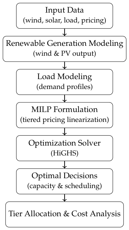
A season-weighted annualized case study with four seasonal typical days was conducted to validate the proposed model. The MILP was implemented in Pyomo and solved using the HiGHS solver. A baseline evaluation, mechanism interpretation, ablation studies, and scenario perturbations were performed to assess effectiveness and extract engineering insights.

5.1. Experimental Set-Up

The case study was based on an islanded expressway service area microgrid located in central China. Due to engineering confidentiality, the exact site name is not disclosed. Nevertheless, the meteorological and load profiles used in this study were constructed from representative regional wind, solar irradiance, and traffic-related demand characteristics so that the case remained reproducible at the methodological level and representative of typical service area operating conditions.

5.1.1. Seasonal Typical Days and Annualization

The seasonal typical days were selected to represent the characteristic operating patterns of spring, summer, autumn, and winter. Each typical day was constructed from representative seasonal renewable generation and load profiles, and the annual objective was obtained by weighting these four typical days according to the number of calendar days in each season. This seasonal typical day approximation was adopted to balance computational tractability and annual representativeness.

Four 24-h typical days representing spring, summer, autumn, and winter were selected. Their annual weights were set according to the number of days each season accounts for: $N_{\mathrm{spring}}=92$, $N_{\mathrm{summer}}=92$, $N_{\mathrm{autumn}}=91$, and $N_{\mathrm{winter}}=90$. The annual objective was strictly annualized using these weights. The high-tier energy ratio was defined as ${\rho }_d^{\mathrm{HT}}=E_d^{\left(3\right)}/E_d^{\mathrm{ex}}\times 100\%$, which quantifies the severity of premium risk on day d by measuring the triggering intensity of the premium tier under tiered settlement.

5.1.2. Base Parameter Settings

(1) Tiered tariff. A three-tier inclining block tariff was adopted. Tier 1 covered 0–3000 kWh with ${\pi }_1=1.00$ RMB/kWh; Tier 2 covered 3000–6000 kWh with ${\pi }_2=1.60$ RMB/kWh; and Tier 3 applied to consumption above 6000 kWh with ${\pi }_3=3.00$ RMB/kWh (premium tier).

(2) Device parameters. Unit investment costs were set to $C_{\mathrm{inv}}^{\mathrm{W}}=4500$ RMB/kW for wind and $C_{\mathrm{inv}}^{\mathrm{PV}}=3000$ RMB/kW for PV. The unit investment cost of storage was $C_E^{\mathrm{ES}}=1500$ RMB/kWh. The planning horizon was $Y=15$ years with a discount rate $r=8\%$. The O&M ratio was $\gamma =2\%$. The storage efficiency was ${\eta }_{\mathrm{bess}}=0.9$, with SOC bounds ${\mathrm{SOC}}_{min}=0.1$ and ${\mathrm{SOC}}_{max}=0.8$.

(3) Forecasted source and load data. The annual capacity factors were set to $C{F}_w=22\%$ and $C{F}_{pv}=18\%$. Seasonal typical day wind–PV generation and load profiles were generated using historical meteorological and traffic flow data. The aggregated EV charging load accounted for approximately 35% of the total demand.

The wind and solar input profiles were derived from historical regional meteorological data, including wind speed and solar irradiance records, while the service area load profiles were constructed from representative traffic flow-related demand and facility electricity consumption characteristics. These data were aggregated into seasonal typical day profiles for annualized optimization.

5.1.3. Ablation Study Settings

To examine the necessity of the key model components, two ablation baselines were considered: no tier and no storage:

(1) No tier. The external electricity price was simplified to a single flat tariff, and the external energy cost was computed linearly with daily purchased energy. This setting removes the cross-tier premium effect. It was used to compare differences in decision structures and risk characterization capability, rather than make a strictly fair comparison of absolute cost levels under different pricing rules.

(2) No storage. All storage-related decision variables and SOC dynamic constraints were removed, and the power balance was satisfied solely by wind–PV generation and external supplementation. This baseline was used to quantify the role of storage in peak shaving and in suppressing high-tier triggering under tiered settlement.

5.1.4. Scenario Settings

To evaluate robustness under engineering perturbations, five scenarios were designed, as summarized in

Table 2. Case scenarios.

Scenario	Name	Thresholds (kWh)	${\overline{\mathit{P}}}_{\mathbf{ext}}^{\left(\mathit{s}\right)}$ (kW)	${\mathit{\pi }}_3^{\left(\mathit{s}\right)}$ (RMB/kWh)	${\mathit{\kappa }}_{\mathbf{PV}}^{\left(\mathit{s}\right)}$	${\mathit{\kappa }}_{\mathbf{W}}^{\left(\mathit{s}\right)}$	${\mathit{\kappa }}_{\mathbf{EV}}^{\left(\mathit{s}\right)}$
1	Baseline	3000/6000	1800	3.0	1.00	1.00	1.00
2	Tighter external limit	3000/6000	1300	3.0	1.00	1.00	1.00
3	Higher Tier-3 price	3000/6000	1800	3.3	1.00	1.00	1.00
4	PV downturn (cloudy)	3000/6000	1800	3.0	0.85	1.00	1.00
5	EV demand increased	3000/6000	1800	3.0	1.00	1.00	1.15
6	Lower thresholds	2400/4800	1800	3.0	1.00	1.00	1.00

. Disturbances were imposed upon four aspects: the external supplementation capacity, premium intensity, renewable availability, and load level. The resulting optimal capacities and economic performance were then compared across scenarios.

In addition to the original five scenarios, a sixth scenario was introduced to examine the sensitivity of the operational pattern to the tier-threshold structure. Specifically, the cumulative energy thresholds of the tiered electricity settlement were tightened from 3000/6000 kWh to 2400/4800 kWh, while all other parameters remained unchanged.

5.2. Baseline Results and Mechanism Analysis

5.2.1. Baseline Optimal Sizing and Cost Breakdown

Under the baseline scenario (Scenario 1), the optimal configuration was obtained as follows: PV capacity $P^{pv}=800$ kW, wind capacity $P^{wt}=800$ kW, storage power capacity $P_{\mathrm{BESS}}^{cap}=155.7$ kW, and storage energy capacity $E_{\mathrm{BESS}}^{cap}=532.7$ kWh. The annualized objective value was $7.6396\times {10}^6$ RMB/year.

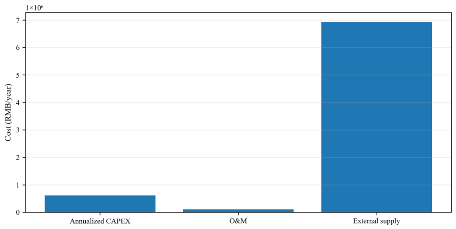
As shown in Figure 3, the external supplementation cost dominated the annualized total cost. The annualized external electricity cost was approximately $6.92\times {10}^6$ RMB/year, accounting for 90.75% of the objective value. The annualized investment (CAPEX) was about $6.01\times {10}^5$ RMB/year (7.87%), while the O&M cost was about $1.18\times {10}^5$ RMB/year (1.54%). This cost structure indicates that improving system economics primarily relies on reducing external energy purchases. The key is to curtail the procurement of high-tier premium energy, rather than marginally reducing investment or routine O&M expenditures.

5.2.2. Tier-Triggering Seasonal Characteristics and Time-of-Day Sources

The statistics of the daily external energy $E_{\mathrm{ex}}$, peak external power $P_{\mathrm{ex}}^{peak}$, renewable supply share, and tier-wise energy allocations are summarized in

Table 3. Typical-day KPIs and tier allocations.

Typical Day	${\mathit{N}}_{\mathit{d}}$ (Day)	${\mathit{E}}_{\mathbf{ex}}$ (kWh/Day)	${\mathit{P}}_{\mathbf{ex}}^{\mathbf{peak}}$ (kW)	Renew. Share (%)	${\mathit{e}}_1$ (kWh)	${\mathit{e}}_2$ (kWh)	${\mathit{e}}_3$ (kWh)	High-Tier Ratio (%)
Spring	92	6220.8	667.4	69.05	3000	3000	220.8	3.55
Summer	92	12,001.3	1018.5	51.01	3000	3000	6001.3	50.01
Autumn	91	9283.9	782.2	56.65	3000	3000	3283.9	35.37
Winter	90	11,410.7	919.9	54.22	3000	3000	5410.7	47.42

.

Table 3 indicates pronounced seasonal heterogeneity in the tier-triggering intensity:

Spring. $E_{\mathrm{ex}}=6220.8$ kWh/day, and the portion exceeding the 6000-kWh threshold was only $e_3=220.8$ kWh/day, corresponding to ${\rho }_d^{HT}=3.55\%$. Meanwhile, the renewable share reached 69.05%, suggesting that wind–PV generation covered a large fraction of the load; therefore, the external supply mainly played a supplemental and smoothing role, and the high-tier contribution was limited.

Summer. $E_{\mathrm{ex}}$ = 12,001.3 kWh/day, with $e_3=6001.3$ kWh/day and ${\rho }_d^{HT}=50.01\%$, meaning that approximately half of the purchased energy fell into the premium tier. Consistently, the renewable share dropped to 51.01%, implying stronger reliance on an external supply under high-load conditions. In addition, $P_{\mathrm{ex}}^{peak}$ was highest in the summer (1018.5 kW), indicating both large external energy and high peak stress.

Autumn. $E_{\mathrm{ex}}=9283.9$ kWh/day, $e_3=3283.9$ kWh/day, and ${\rho }_d^{HT}=35.37\%$. External supplementation remained substantial, while the high-tier share was lower than in summer, representing a partially controllable premium risk level.

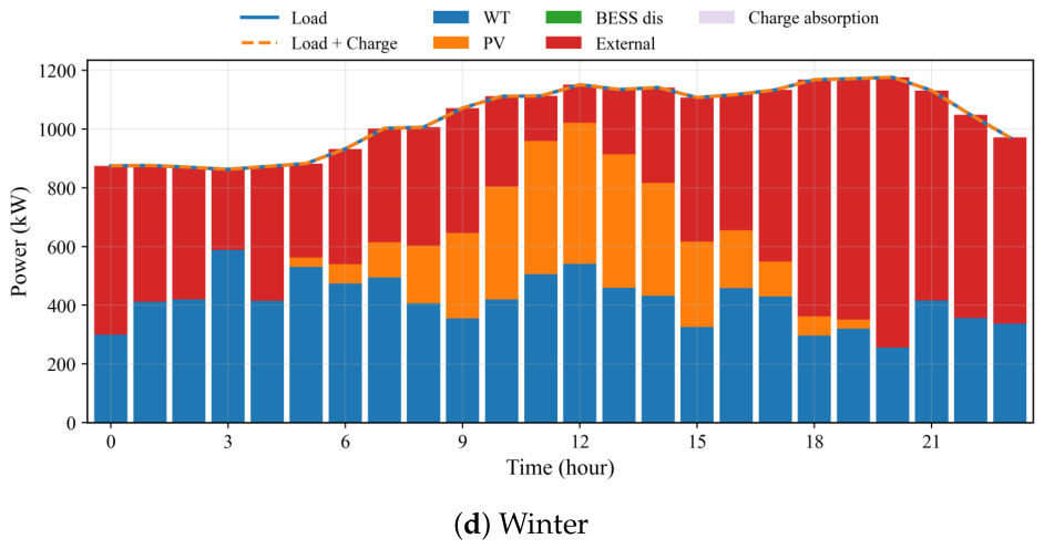
Winter. $E_{\mathrm{ex}}$ = 11,410.7 kWh/day, $e_3=5410.7$ kWh/day, and ${\rho }_d^{HT}=47.42\%$. Although the renewable share in winter (54.22%) was higher than that in summer, poorer temporal matching between the demand and renewable availability—especially the overlap of the evening peaks with renewable troughs—forced the external supply to increase during critical hours, leading to persistent high-tier triggering.

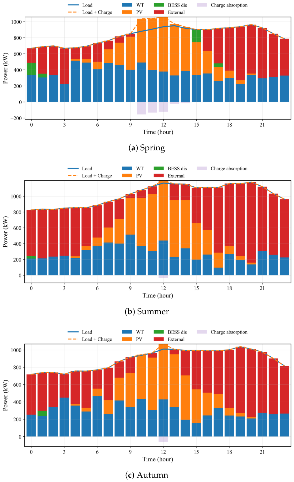
To reveal the time-of-day sources of tier triggering, Figure 4 reports the hourly power-balance decomposition for the four seasonal typical days. Wind (WT) is shown by the blue bars, PV is shown by the orange bars, external supply is shown by the red bars, BESS discharge is shown by the green bars, and charge absorption (negative charging) is shown in purple. The solid line denotes the load, while the dashed line represents the equivalent demand of load plus charging.

According to Figure 4, $e_3$ was not accumulated uniformly across the day; instead, it was mainly driven by an elevated external supply during evening peak demand hours when renewable generation declined. During the daytime (from approximately 9:00 a.m. to 3:00 p.m.), the PV output increased noticeably, and the external supply decreased simultaneously. Charging absorption appeared, indicating that the optimizer tends to exploit renewable-rich hours to increase local utilization and charge the battery, thereby reducing external purchases and slowing the growth of cumulative external energy. During the evening and into the night (from approximately 5:00 p.m. to 10:00 p.m.), demand was high, while renewables dropped. The external supply rose and remained high for a sustained period. When battery energy was limited, discharge could only partially compensate for it, making the external supply the dominant source and causing the cumulative purchased energy to exceed 6000 kWh more easily, thereby enlarging $e_3$.

Therefore, tiered settlement exerted a clear shaping effect on the optimal operating strategy; the optimizer systematically searched for operating trajectories that reduced the high-tier energy (charge during renewable-rich hours, discharge during evening peaks, and suppress both external peak power and cumulative external energy). However, when the system relied heavily on an external supply (e.g., summer and winter), the available flexibility became insufficient, and a relatively large $e_3$ remained unavoidable.

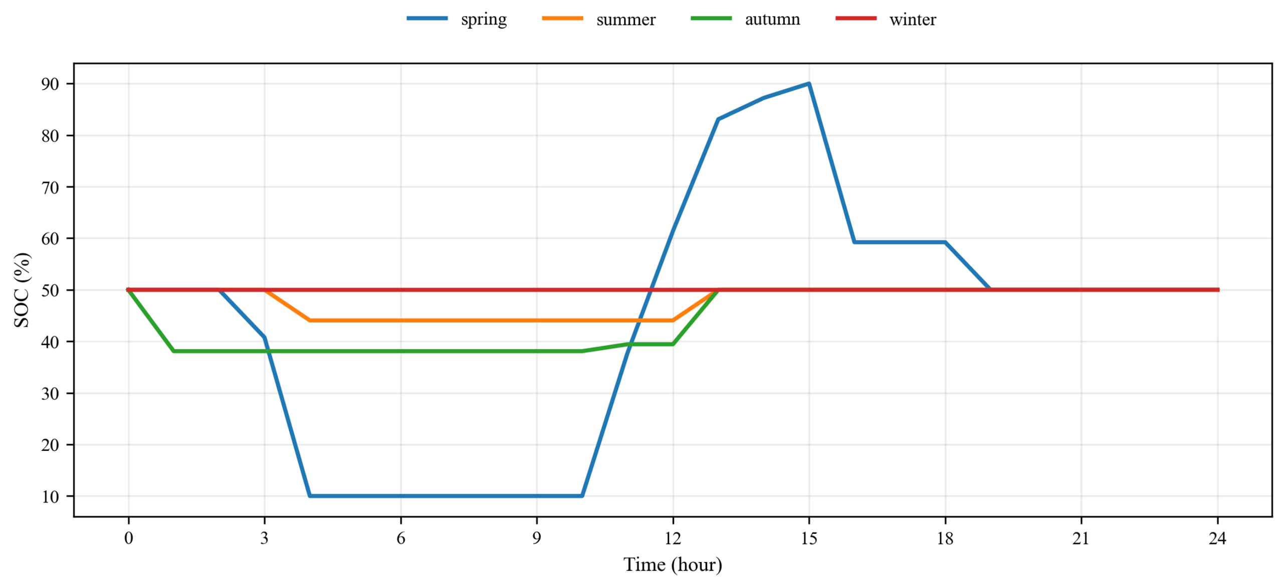
To further characterize the intraday battery strategy, Figure 5 presents the SOC trajectories.

The SOC followed a typical charge-then-discharge pattern; it increased during renewable-rich daytime hours and decreased during evening peaks, supporting the load and reducing the external peak power.

It should be emphasized that entering the high-tier segment was determined by whether the daily cumulative purchased energy exceeded the threshold, rather than solely by whether the external peak was shaved. Since $E_{\mathrm{ex}}$ in summer and winter far exceeded 6000 kWh, the current storage scale could only reduce part of the external energy and the high-tier share and could not fully eliminate $e_3$. This implies that systematic reduction of premium-segment energy requires a combination of structural measures: (1) increasing effective renewable coverage of demand, (2) enhancing transferable energy flexibility (e.g., larger $E_{\mathrm{BESS}}^{cap}$ or flexible loads and demand response), and (3) optimizing charge and discharge timing under settlement constraints so that more external energy is allocated to Tiers 1–2 rather than Tier 3.

5.3. Ablation Study Results

The ablation results in

Table 4. Ablation results.

Setting	${\mathit{P}}^{\mathbf{pv}}$ (kW)	${\mathit{P}}^{\mathbf{wt}}$ (kW)	${\mathit{P}}_{\mathbf{BESS}}^{\mathbf{cap}}$ (kW)	${\mathit{E}}_{\mathbf{BESS}}^{\mathbf{cap}}$ (kWh)	High Tier (%)	Objective (RMB/yr)
Full model (tier + storage)	800	800	155.7	532.7	34.01	$7.6396\times {10}^6$
No tier (flat price)	800	800	33.3	39.6	–	$4.2326\times {10}^6$
No storage	800	800	0	0	35.63	$7.6982\times {10}^6$

verify the necessity of endogenous tiered modeling and coordinated storage operation.

No tier. The annualized cost decreased to $4.2326\times {10}^6$ RMB/year, while storage shrank drastically (33.3 kW power and 39.6 kWh energy). In this setting, the model lost the ability to characterize premium risk (e.g., it could not produce the high-tier ratio), and it tended to substitute external purchases for storage flexibility; consequently, it provideed limited guidance for tier-driven engineering decisions.

No storage. The annualized cost increased to $7.6982\times {10}^6$ RMB/year, and the high-tier ratio rose to 35.63%. Without intraday energy shifting, the external supply profile became more rigid, and the cross-tier avoidance capability was lost, confirming that storage is a key flexibility resource for suppressing tier-triggered premiums.

5.4. Scenario Perturbation Analysis

The optimization results for Scenarios 1–5 are summarized in

Table 5. Optimization results in different scenarios.

Scen.	Name	${\mathit{P}}^{\mathbf{pv}}$ (kW)	${\mathit{P}}^{\mathbf{wt}}$ (kW)	${\mathit{P}}_{\mathbf{BESS}}^{\mathbf{cap}}$ (kW)	${\mathit{E}}_{\mathbf{BESS}}^{\mathbf{cap}}$ (kWh)	High-Tier (%)	Objective (RMB/yr)
1	Baseline	800	800	155.7	532.7	34.01	$7.6396\times {10}^6$
2	Tighter external limit	800	800	155.7	532.7	34.01	$7.6396\times {10}^6$
3	Higher Tier-3 price	800	800	155.7	532.7	34.01	$8.0471\times {10}^6$
4	PV downturn (cloudy)	800	800	74.0	153.8	39.13	$8.3625\times {10}^6$
5	EV demand increased	800	800	141.2	409.4	36.79	$8.0411\times {10}^6$

. An additional threshold sensitivity case (Scenario 6) is discussed separately in Section 5.6 to further examine the effect of the tier-threshold structure.

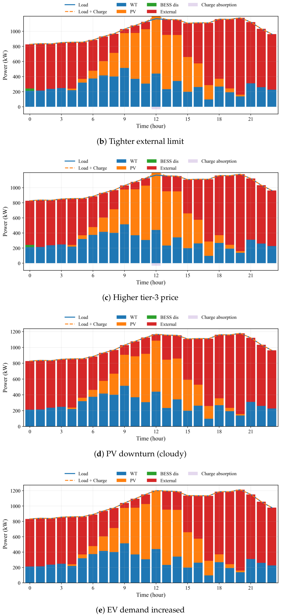
Scenario 2: Tighter external limit. When the external power limit decreased from 1800 kW to 1300 kW, both the optimal capacities and the objective remained nearly unchanged. This is because the baseline peak external power was about 1018.5 kW (Table 3), not reaching 1300 kW. Hence, the constraint was inactive in this range and did not drive reoptimization.

Scenario 3: Higher Tier-3 price. Increasing the Tier-3 unit price from 3.0 to 3.3 RMB/kWh raised the objective to $8.0471\times {10}^6$ RMB/year. Since the high-tier share was already 34.01% in the baseline, a higher premium price directly amplified the marginal cost of $e_3$, strengthening the economic incentive to reduce high-tier energy and demonstrating the leverage effect of tiered settlement on the annual cost.

Scenario 4: PV downturn. With a PV scaling factor ${\kappa }_{\mathrm{PV}}^{\left(4\right)}=0.85$, the objective increased to $8.3625\times {10}^6$ RMB/year, and the high-tier ratio rose to 39.13%. Reduced daytime renewables led to earlier and larger external purchases, causing the cumulative purchased energy to cross the 6000-kWh boundary sooner and expand $e_3$. Meanwhile, the reduced battery energy capacity suggests that under resource scarcity, the system prefers relying on external supply rather than enlarging intraday energy shifting.

Scenario 5: EV demand increased. With ${\kappa }_{\mathrm{EV}}^{\left(5\right)}=1.15$, the objective increased to $8.0411\times {10}^6$ RMB/year, the high-tier ratio rose to 36.79%, and $E_{\mathrm{BESS}}^{cap}$ increased to 409.4 kWh. Demand growth forced the system to allocate more adjustable energy to shave peaks and slow the growth of cumulative purchases, thereby partially mitigating high-tier triggering.

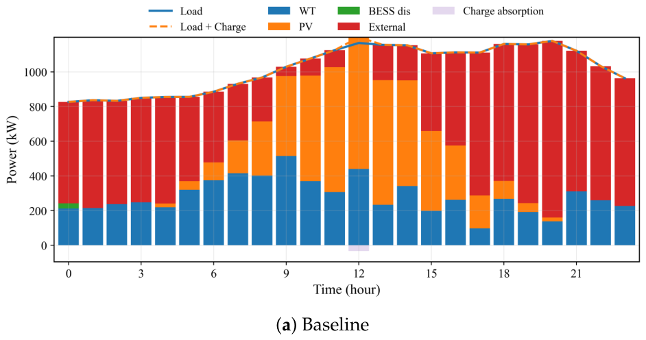
Figure 6 compares the hourly operation under different scenarios (typical summer day, as an example).

Scenarios 1–3 exhibited nearly overlapping profiles, confirming that Scenario 2 was inactive and Scenario 3 mainly affected cost through the tariff parameter without substantially changing the power-balance pattern. In Scenarios 4 and 5, the external supply increased across multiple hours—especially during evening peaks—which was the direct source of increased high-tier energy. When demand increased (Scenario 5), storage actions intervened more frequently, reflecting stronger intraday energy shifting to hedge external peaks and cumulative purchases.

This observation suggests that under the baseline cumulative demand structure, changing the Tier-3 price mainly affected the total cost level, whereas the threshold settings played a more direct role in altering the timing and intensity of premium-tier triggering.

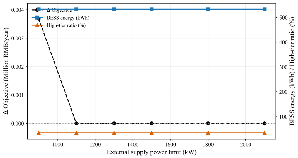
5.5. Sensitivity to External Supplementation Capacity

To assess the impact of the external supplementation capacity on planning outcomes, a sensitivity analysis with respect to $P_{\mathrm{ex}}^{max}$ was performed, as shown in Figure 7.

As shown in Figure 7, both the high-tier ratio and the battery energy capacity remained nearly unchanged when the external supply limit was above the natural peak external demand, whereas the objective value only exhibited a noticeable increase when the limit was tightened to 900 kW. This further confirms the existence of a threshold effect in external supplementation capacity planning.

The results show that when $P_{\mathrm{ex}}^{max}$ decreased gradually from 2100 kW to 1100 kW, the objective variation remained close to zero, while the battery energy capacity and the high-tier ratio were nearly unchanged. In this region, the natural peak external demand stayed below the limit; therefore, the external capacity did not form a bottleneck, and increasing the limit yielded a limited marginal benefit.

When $P_{\mathrm{ex}}^{max}$ further decreased to 900 kW, the objective increased (approximately $7.6433\times {10}^6$ RMB/year), and both the storage sizing and the high-tier ratio changed. This indicates that the external limit became active as it approached or fell below the peak external demand. The system must compensate for an insufficient external capability through stronger internal regulation (restructuring charge and discharge timing and increasing effective renewable utilization), which triggers reoptimization of both the cost and capacity.

Overall, external capacity planning exhibited a clear threshold effect: (1) when $P_{\mathrm{ex}}^{max}$ was higher than the natural peak external demand, the marginal benefit of further expansion was limited, and (2) when $P_{\mathrm{ex}}^{max}$ was below the peak demand, internal flexibility requirements and the total cost increased significantly, and the tier-triggered premium risk may have been amplified. These findings suggest that the proposed model can be used to back-calculate an economically reasonable range for the external access capacity, enabling integrated decisions that couple access capacity, storage sizing, and settlement risk.

5.6. Sensitivity to Tier Thresholds

To further examine the effect of the tier-threshold structure on system operation, an additional sensitivity analysis was conducted by tightening the cumulative energy thresholds of the tiered electricity settlement. Specifically, the original thresholds of 3000 and 6000 kWh were reduced to 2400 and 4800 kWh, while all other parameters were kept unchanged within this sensitivity test.

It should be noted that this threshold sensitivity test was conducted as an additional mechanism-oriented analysis under the same optimization framework, but its baseline values were reported separately from the main case study baseline in order to highlight the isolated impact of threshold tightening. Therefore, the numerical values in this subsection are not intended to replace the baseline configuration reported in Section 5.2.

The results are summarized in

Table 6. Sensitivity analysis with respect to tier thresholds.

Case	Tier-1 Threshold (kWh)	Tier-2 Threshold (kWh)	${\mathit{P}}_{\mathbf{BESS}}^{\mathbf{cap}}$ (kW)	${\mathit{E}}_{\mathbf{BESS}}^{\mathbf{cap}}$ (kWh)	High-Tier Ratio(%)	Objective (RMB/yr)
Baseline thresholds	3000	6000	500.0	825.5	24.7	$6.4014\times {10}^6$
Higher Tier-3 price	3000	6000	500.0	825.5	24.7	$6.6610\times {10}^6$
Tightened thresholds	2400	4800	500.0	825.5	39.0	$7.1178\times {10}^6$

. When only the Tier-3 price was increased, the high-tier ratio remained unchanged at 24.7%, while the annualized objective value rose from $6.4014\times {10}^6$ RMB/year to $6.6610\times {10}^6$ RMB/year. In contrast, when the thresholds were tightened, the high-tier ratio increased substantially to 39.0%, and the annualized objective value further rose to $7.1178\times {10}^6$ RMB/year.

These results indicate that the threshold structure had a stronger impact on premium-tier triggering than the Tier-3 price alone. In other words, price variation mainly affected the cost level, whereas threshold tightening directly changed how early cumulative external electricity purchases entered the premium tier. This additional experiment further demonstrated that the proposed framework can capture the threshold-triggering effect of cumulative tiered settlement, which cannot be reflected under conventional linear pricing models.

Scenarios 1–5 correspond to the main case studies summarized in Table 5, whereas the threshold sensitivity case is discussed separately in this subsection to avoid mixing the primary performance comparison with an auxiliary mechanism analysis case.

6. Conclusions

This paper proposed a joint capacity sizing and operation optimization model for islanded wind–PV–battery systems at expressway service areas under tiered electricity pricing. By reformulating the nonlinear tiered settlement rule into an equivalent piecewise-linear representation, the tiered pricing mechanism was embedded endogenously into the optimization framework, thereby enabling integrated planning and operational decision making.

Based on the season-weighted annualized case study with four seasonal typical days, the major findings can be summarized as follows:

(1)

Under the baseline scenario, the optimal configuration obtained was 800 kW PV, 800 kW wind, 155.7 kW battery power capacity, and 532.7 kWh battery energy capacity, with an annualized objective value of $7.6396\times {10}^6$ RMB/year. These results confirm that the proposed framework can simultaneously determine economically favorable renewable and storage capacities while coordinating hourly operation under tiered settlement.

(2)

External electricity supplementation dominated the overall cost structure. In the baseline case, the annualized external electricity cost was approximately $6.92\times {10}^6$ RMB/year, accounting for 90.75% of the total objective value. This indicates that the key to improving system economics lies primarily in reducing cumulative external electricity purchases, especially those entering the premium tier, rather than in marginal reductions in capital investment or routine O&M costs.

(3)

Premium risk exhibited strong seasonal heterogeneity. The high-tier ratio reached 50.01% in summer and 47.42% in winter, while it was only 3.55% in spring and 35.37% in autumn. The results show that summer and winter are the most critical periods for tier-triggered premium cost accumulation, mainly due to lower renewable coverage and poorer temporal matching between renewable generation and load demand during evening peak hours.

(4)

Battery storage plays a significant role in suppressing cumulative tier triggering. Compared with the full model, the no-storage case increased the annualized objective value to $7.6982\times {10}^6$ RMB/year and raised the high-tier ratio to 35.63%, confirming that storage contributes not only to conventional peak shaving and valley filling but also to premium risk mitigation by reducing the amount of electricity allocated to the highest pricing tier.

(5)

Scenario analysis further demonstrated that renewable deterioration and load growth were the main drivers of premium-risk amplification. Specifically, under the PV downturn scenario, the annualized objective increased to $8.3625\times {10}^6$ RMB/year, and the high-tier ratio rose to 39.13%. Under the EV demand increase scenario, the annualized objective became $8.0411\times {10}^6$ RMB/year, and the high-tier ratio reached 36.79%. These findings highlight the necessity of jointly considering renewable uncertainty, demand growth, and tariff structure in service area energy planning.

(6)

The proposed framework is primarily intended for islanded expressway service area microgrids and similar medium- and low-voltage integrated energy systems with bounded external supplementation. Although the idea of embedding cumulative tiered settlement into optimization is general, direct application to high-voltage bulk power systems would require substantial reformulation to incorporate detailed network topology, AC power flow, reserve requirements, and reactive power interactions.

Overall, the essential contribution of this work lies in transforming tiered electricity settlement from an exogenous post-calculation rule into an endogenous optimization driver. In this way, the proposed method provides a practical and interpretable tool for capacity planning and hourly operation of islanded expressway service area microgrids under cumulative tiered pricing.

Future work will focus on several extensions of the present framework, including the incorporation of battery degradation models, explicit reserve constraints, active power loss modeling, and demand response strategies. In addition, multi-service area coordinated optimization, uncertainty-aware multi-stage scheduling, and detailed power flow-based validation will be investigated to further improve the applicability of the proposed approach in large-scale practical systems.