Research on Multi-Time-Scale Optimal Control Strategy for Microgrids with Explicit Consideration of Uncertainties

Abstract

Distributed generation (DG) exhibits inherent volatility and intermittency, and its grid-integration expansion presents formidable challenges to microgrid regulation and control. Conventional control strategies often neglect the uncertainties associated with renewable energy generation and the coordinated management of flexible resources. This paper proposes a multi-time-scale optimal control strategy for microgrids that explicitly accounts for uncertainty. The strategy integrates a collaborative scheduling framework for assets, including electric vehicles (EVs) and energy storage systems, alongside a stochastic optimization model for microgrids that comprehensively incorporates uncertainties from wind and solar power generation, EV operations, and load forecasting errors. The improved Archimedean chaotic adaptive whale optimization algorithm is utilized to solve the optimal scheduling model, while the Latin hypercube sampling (LHS) technique is employed to address uncertainty-related problems in the optimization process. Case study results demonstrate that, in comparison with traditional optimal scheduling strategies, the proposed approach more effectively mitigates uncertainties in real-world operations, reduces microgrid operational risks, achieves a significant reduction in scheduling costs, and concurrently fulfills the dual objectives of microgrid economic efficiency and operational security.

1. Introduction

Against the backdrop of the global energy transition and sustainable development, the power system is undergoing a paradigm shift from traditional centralized generation to DG configurations. This transformation has profoundly reshaped the structure and operational paradigm of power grids [1]. At the distribution network level, the escalating integration of distributed energy resources (DERs) introduces challenges, including power flow congestion, voltage limit violations, degraded power quality, and diminished grid regulation capability. To address the challenges brought by rising renewable penetration and increasingly complex control requirements, advanced microgrid and hybrid renewable energy system architectures have emerged as effective solutions for improving flexibility, reliability, and renewable energy utilization [2,3].

As small-scale power systems embedded within distribution networks, microgrids not only accommodate distributed generation but also enable bidirectional energy exchange with the main grid. By coordinating multiple renewable sources and storage through an effective energy management strategy, smart microgrids can achieve flexible power balancing and bidirectional regulation, thereby improving operational reliability, power quality, and economic performance [4]. Therefore, to achieve optimal regulation and operation of distribution networks integrated with multiple microgrid clusters, in-depth research on the collaborative optimization and control strategies between microgrids and distribution networks holds significant theoretical and practical value.

Existing energy management approaches for microgrids primarily fall into two categories: day-ahead planning and time-sequential rolling optimization. Day-ahead planning refers to the process where the energy management system derives an optimal power allocation strategy for the next day based on forecasts of renewable energy output and load demand. Reference [5] developed a two-stage distributionally robust optimal scheduling model. Reference [6] proposed a short-term energy dispatch model integrated with a hybrid energy storage system, aiming to improve the economic performance of integrated energy systems. Reference [7] presented a modified microgrid dispatch method that accounts for the decision-making behavior of air conditioning users, incorporating dynamic load-side decisions. Reference [8] employed the Monte Carlo method and demand response to address supply–demand uncertainties. Reference [9] developed a model predictive control strategy for microgrid optimal dispatch, integrating thermostatically controlled loads into the demand-side management system to enhance system flexibility. According to the above-mentioned literature, it can be seen that most of the existing microgrid control strategies only optimize for one type of load resource, and there are significant deficiencies in the coordinated scheduling and optimization among multiple energy systems, which leads to problems such as low energy utilization efficiency and poor economic performance within the grid.

Intra-day dispatch methods based on receding-horizon rolling optimization work by repeatedly solving an optimal control problem at each decision step—planning the next actions and correcting in real time—to produce a dynamically updated dispatch schedule. Reference [10] proposed a multi-time-scale framework for electricity–hydrogen microgrids, modeling coupling dynamics and constraints. Reference [11] developed an MPC-based dispatch framework for microgrids with electric vehicles, incorporating EV availability and charging flexibility. Reference [12] introduced a Stackelberg game-theoretic strategy for demand response, using logistic functions and fuzzy chance constraints to handle participation uncertainty. Reference [13] designed a two-layer energy management system: MPC for economic scheduling and MILP for precise power tracking. Reference [14] presented an adaptive EMS that combines cost-aware day-ahead scheduling with intra-day rescheduling triggered by forecast updates or events. Reference [15] proposed a modular multi-time-scale control architecture for DC microgrids, improving adaptability and scalability under changing conditions. However, most of the aforementioned studies focus on multi-objective collaborative control methods based on convergence algorithms, with a notable gap in research on source–load–storage matching within low-voltage distribution networks. Concurrently, existing dispatch strategies predominantly prioritize improving the overall efficiency of distribution networks, while overlooking the microgrid’s demand for renewable energy integration.

When microgrids operate independently of the distribution network, how to maximize the benefits between the two has become a focus of current research both at home and abroad. Reference [16] proposed a probabilistic energy management method for multi-microgrid systems considering energy storage systems, achieving simultaneous optimization of operating costs and system reserves. Reference [17] presented an optimal scheduling method for source–storage–load in DC microgrids based on virtual bus voltage control, aiming to maximize economic benefits. Reference [18] proposed a cross-scale coupling enhanced scheduling optimization method for microgrids with hybrid energy storage systems. Reference [19] proposed a distributed economic model predictive control algorithm for microgrid cluster dispatch, reducing economic loss and communication burden. However, the optimal control schemes and economic dispatch schemes proposed in the above references are mostly based on the steady-state operation of microgrids, with precise and reliable information on the input of new energy and loads, thereby ignoring the uncertainty factors of renewable energy generation and adjustable loads in the actual operation of microgrids.

To address the identified research gaps, this paper proposes a multi-time-scale microgrid dispatch framework covering day-ahead, intra-day, and real-time horizons. It coordinates energy regulation across time scales to optimize and balance microgrid energy supply. A dynamic optimization model is formulated to minimize operational costs and maximize renewable energy absorption. The model is solved using an Archimedean chaotic adaptive whale optimization algorithm. To handle uncertainties in renewable generation, EV behavior, and load forecasts, a stochastic optimal control strategy is developed—yielding chance constraints with random parameters. These are converted into deterministic constraints via Latin hypercube sampling-based chance-constrained programming, transforming the problem into a mixed-integer linear program. Numerical experiments validate the algorithm’s correctness, efficiency, and robustness.

2. Research on Multi-Time-Scale Optimal Dispatch of Microgrids Based on an Improved Whale Optimization Algorithm

As distributed energy resources and electric vehicles become increasingly integrated into microgrids, the resulting uncertainty and operational coupling have made energy management more challenging [20]. Existing research predominantly focuses on single-time-scale optimization; however, the inherent volatility of DG and the rapid dynamics of user demand often result in substantial deviations between pre-formulated dispatch schemes and actual operating conditions, thereby impeding the optimal performance of microgrids.

This paper proposes a multi-time-scale microgrid dispatch framework, which aims to effectively reduce operational costs and maximize renewable energy accommodation through the collaborative management of day-ahead, intra-day, and real-time scheduling. Building upon this framework, an improved Archimedean chaotic adaptive whale optimization algorithm is introduced. This integrated strategy is designed to enhance the precision and efficiency of microgrid dispatch, thereby achieving an optimal system operating state.

2.1. Multi-Time-Scale Regulation Framework

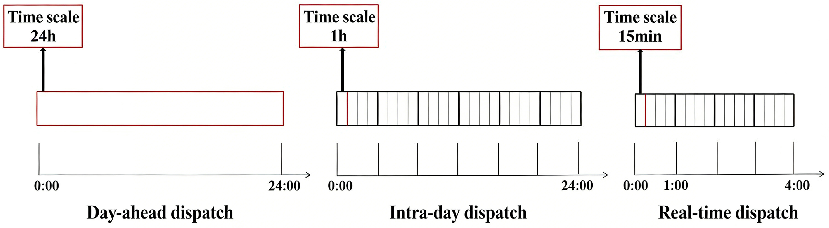
In the day-ahead stochastic optimal dispatch stage, which is executed once every 24 h, optimized load data are integrated—including forecasts of the day’s EV charging demand, heat pumps, energy storage devices, and the main grid. The objective is to determine the power purchase and sale requirements for each time interval of the following day, with the aims of minimizing microgrid operational costs, maximizing renewable energy accommodation, and achieving a tight alignment between the load curve and the renewable energy generation curve.

In the real-time rolling optimal dispatch phase, it relies on the ultra-short-term prediction information of each component and adopts a dynamic optimization strategy to search for and execute the optimal power distribution plan in real time. As the prediction time window advances, information is constantly updated, which ensures the real-time accuracy of the scheduling plan. The overall framework of the proposed multi-time-scale optimal dispatch strategy is illustrated in Figure 1.

2.2. Multi-Time-Scale Optimal Regulation Model for Microgrids

(1)

Day-Ahead Scheduling Model

Day-ahead scheduling based on optimization uses forecasted load information to allocate the output of controllable units, thereby smoothing power fluctuations in the microgrid [21]. Decision variables include optimized load, EV charging demand, boiler output, energy storage charge/discharge, and main grid power exchange. Day-ahead scheduling based on optimization uses forecasted load information to allocate the output of controllable units, thereby smoothing power fluctuations in the microgrid. The objective function is as follows:

$$f_1=\min \left\{C_{om}^I+C_{loss}^{ES}+C_{\cos t,1}^{EV}+C_{loss}^{EB}+C_{Grid}\right\}$$

(1)

$$f_2=\min \left\{{\displaystyle \frac{1}{\mathrm{T}}}{\displaystyle \sum _{t=1}^T{P}_{load}^{\prime }}\left(t\right)\right\}$$

(2)

In the formula, $f_1$ represents the operating cost of the microgrid; $C_{om}^I$ is the total operation and maintenance cost of all dispatchable units within the microgrid; $C_{loss}^{ES}$ is the loss cost of energy storage charging and discharging; $C_{\cos t,1}^{EV}$ is the discharge subsidy provided by the microgrid system to EVs for the day-ahead period; $C_{loss}^{EB}$ is the loss cost of the electric boiler; $C_{Grid}$ is the electricity purchase price; $f_2$ is the net load value of the microgrid; and $P_{load}^{\prime }\left(t\right)$ is the net load of the microgrid at time t after the optimization of the source–storage layer.

$${\mathrm{C}}_{\mathrm{om}}^{\mathrm{I}}\left(t\right)={\lambda }_{wt}\cdot P_{wt}\left(t\right)+{\lambda }_{p\nu }\cdot P_{p\nu }\left(t\right)+{\lambda }_{ES}\cdot P_{ES}\left(t\right)$$

(3)

In the formula, ${\lambda }_{wt},{\lambda }_{p\nu },{\lambda }_{ES}$ respectively represent the operation and maintenance cost coefficients of wind turbines, photovoltaic and energy storage; $P_{wt}\left(t\right),P_{p\nu }\left(t\right),P_{ES}\left(t\right)$ respectively represent the output magnitudes of wind turbines, photovoltaic and energy storage at time t.

$${\mathrm{C}}_{\mathrm{loss}}^{\mathrm{ES}}\left(t\right)=\left|P_{ES}\left(t\right)\right|\cdot {\rho }_{ES}$$

(4)

In the formulation, ${\rho }_{ES}$ represents the standard for energy storage loss cost.

$${\mathrm{C}}_{\cos t,1}^{EV}=\left|{\displaystyle \sum _{t=1}^T{P}_1^{EV}}\left(t\right)\cdot p_1^{e\nu }\right|,P_1^{EV}\left(t\right)\le 0$$

(5)

In the formula, $P_1^{EV}\left(t\right)$ represents the output size of the EV at time t in the day-ahead period; and $p_1^{e\nu }$ is the uniform subsidy price for the discharge of the EV in the day-ahead period.

$${\mathrm{C}}_{\mathrm{loss}}^{\mathrm{EB}}\left(t\right)=\left|P_{EB}\left(t\right)\right|\cdot {\rho }_{EB}$$

(6)

In the formula, $P_{EB}\left(t\right)$ represents the output power of the electric boiler at time t; and ${\rho }_{EB}$ is the loss cost of the electric boiler.

$${\mathrm{C}}_{G\mathrm{r}\mathrm{i}\mathrm{d}}(t)=P_{G\mathrm{r}\mathrm{i}\mathrm{d}}(t)\cdot f_{G\mathrm{r}\mathrm{i}\mathrm{d}}$$

(7)

In the formula, $P_{G\mathrm{r}\mathrm{i}\mathrm{d}}(t)$ represents the interactive power between the microgrid and the main grid at time t. ${\mathrm{C}}_{G\mathrm{r}\mathrm{i}\mathrm{d}}(t)$ is positive when the main grid supplies power to the microgrid and negative when the microgrid sells power to the main grid. $f_{G\mathrm{r}\mathrm{i}\mathrm{d}}$ is the unit price of power purchase between the microgrid and the main grid.

$$P_{load}^{\prime }(t)=P_{load}(t)-P_{pv}(t)-P_{wt}(t)+P_{ES}(t)+P_1^{EV}(t)+P_I^{ES}(t)$$

(8)

In the formula, $P_{load}^{\prime }(t)$ represents the net load of the microgrid at time t after the source and storage layer optimization; and $P_{load}(t)$ represents the net load of the microgrid at time t after the load layer optimization.

(2)

Intra-Day Scheduling Model

Intra-day scheduling leverages ultra-short-term forecasts of load and renewable energy generation (with a 1 h rolling horizon) and takes day-ahead scheduling results as the baseline to adjust the output of each controllable unit on an hourly rolling basis [22]. The objective function is formulated as follows:

$$f_1=\min \left\{C_{om}^I+C_{loss}^{ES}+C_{\cos t,2}^{EV}+C_{loss}^{EB}+C_{Grid}\right\}$$

(9)

$$f_2=\min \left\{{\displaystyle \frac{1}{T}}{{\displaystyle \sum _{t=1}^T{P}_{\mathrm{load}}}}^{\prime }(t)\right\}$$

(10)

In the formula, $f_1$ represents the operating cost of the microgrid; $f_2$ represents the net load value of the microgrid; and $C_{\cos t,2}^{EV}$ represents the discharge subsidy provided by the microgrid to EVs within the day.

$$C_{\cos t,2}^{EV}=\left|{\displaystyle \sum _{t=1}^T{P}_2^{EV}}(t)\cdot p_2^{ev}\right|,P_2^{EV}(t)\le 0$$

(11)

In the formula, $P_2^{EV}\left(t\right)$ represents the output size of EV within a day; and $p_2^{ev}$ is the uniform subsidy unit price for the discharge of EV by the microgrid on a daily basis.

(3)

Real-Time Dispatch Model

Real-time dispatch targets renewable energy and load with ultra-small prediction errors, which are dominated by small-scale stochastic fluctuations. Based on real-time forecasting results, the output of each unit is adjusted to align the actual unit operating costs with the daily rolling optimization costs. This approach not only adapts to the volatility of renewable energy but also ensures the optimal economic operation of the entire system.

Real-time dispatch is an online optimization task continuously requiring immediate generation of scheduling decisions [23]. The real-time dispatch objective function is expressed as follows:

$$f_1=\min \left\{C_{om}^I+C_{loss}^{ES}+C_{loss}^{EB}+C_{Grid}\right\}$$

(12)

$$f_2=\min \left\{{\displaystyle \frac{1}{T}}{\displaystyle \sum _{t=1}^T{P}_{\mathrm{load}}^{″}}(t)\right\}$$

(13)

In the formula, $f_1$ represents the operating cost of the microgrid; and $f_2$ represents the net load value of the microgrid.

$$P_{\mathrm{load}}^{″}(t)=P_{\mathrm{lcad}}(t)-P_{pv}(t)-P_{wt}(t)+P_{ES}(t)+P_1^{EV}(t)+P_2^{EV}(t)+P_I^{SL}(t)+P_{II}^{SL}(t)+P_{III}^{SL}(t)$$

(14)

2.3. Solution Strategy for Optimal Dispatch Based on Improved Whale Optimization Algorithm

The whale optimization algorithm (WOA) mimics the humpback whale’s bubble-net feeding behavior. Each whale’s position represents a candidate solution, and its fitness reflects the objective function value. In each iteration, whales update positions by encircling the current best solution or moving along logarithmic spirals. High-fitness individuals progressively guide the search, driving convergence toward the global optimum.

This paper proposes an improved Archimedean chaotic adaptive whale optimization algorithm. It replaces the standard logarithmic spiral in WOA with an Archimedean spiral, employs tent mapping to diversify the initial population, and dynamically adjusts key parameters to strengthen early-stage global exploration. Consequently, the improved algorithm provides greater local search precision, faster global convergence, and better optimization stability [24].

2.3.1. Equidistant Spiral Trajectory Tracking

The equidistant spiral line is mathematically defined by the Archimedean spiral. Its constant radial spacing enables dense, uniform coverage of adjacent solution space—particularly advantageous for fine-grained local optimization. The spiral is generated by rotating at a fixed angular velocity about a central point, with its spacing directly controlled by a tunable parameter.

$$\left\{\begin{array}{c}x=(a+b\cdot l)\cdot \cos (2\pi l)\\ y=(a+b\cdot l)\cdot \sin (2\pi l)\end{array}\right.$$

(15)

$$\overline{{\mathrm{X}}^{\prime }}(t+1)={\left(\overline{D^{\prime }}bl\right)}^4\cdot l\cdot \sin (2\pi l)+\overline{X^{*}}(t)$$

(16)

In the context, $\overline{D^{\prime }}$ represents the distance that the current population needs to move, $\overline{X^{*}}(t)$ represents the global optimal solution calculated in the t-th generation, $a,b,l$ stand for the spiral parameter, and $\overline{{\mathrm{X}}^{\prime }}(t+1)$ indicates the solution in the t + 1-th generation.

2.3.2. Tent Map-Optimized Initial Population Distribution

This paper proposes a tent map-based initial population generation method to enhance population diversity and improve algorithmic solution efficiency, thereby laying a diverse foundation for the algorithm’s global optimization capability.

$$Z_{k+1}=\left\{\begin{array}{cc}{Z}_k/\beta & Z_k\in (0,\beta ]\\ \left(1-Z_k\right)/\left(1-\beta \right)& Z_k\in (\beta ,1]\end{array}\right.$$

(17)

In the formula, k represents the current population size, $Z_k$ has an initial value of 0.152, and $\beta$ is a chaotic parameter with an initial value of 0.4, which exhibits good randomness and can prevent the generation of divergent sequences.

2.3.3. Adaptive Parameter Regulation Strategy

This paper proposes an adaptive parameter optimization method that enhances global optimality through dynamic parameter regulation and integrates the WOA to improve convergence performance without sacrificing convergence reliability.

In the conventional WOA, the control parameter a usually decreases linearly with the iteration number, which may lead to insufficient exploration and premature convergence. In this study, the parameter a is updated adaptively according to the iteration progress, so that the probability of generating |A| > 1 is increased in the early stage, thereby expanding the global search range, while the probability of generating |A| < 1 is increased in the latter stage to enhance local search around the current best solution.

The adaptive update of a is defined as follows:

$$a=\left(a_{\max }-a_{\min }\right)\cdot \cos \left({\displaystyle \frac{\pi }{2}}\cdot {\displaystyle \frac{t}{T_{\max }}}\right)$$

(18)

where $a_{\max }$ and $a_{\min }$ denote the maximum and minimum values of the control parameter a, respectively, t is the current iteration number, and $T_{\max }$ is the maximum number of iterations. Through this adaptive update mechanism, the search behavior of whale individuals is dynamically regulated during the optimization process, which improves the balance between exploration and exploitation.

2.3.4. Algorithmic Procedure of the Improved Whale Optimization Algorithm

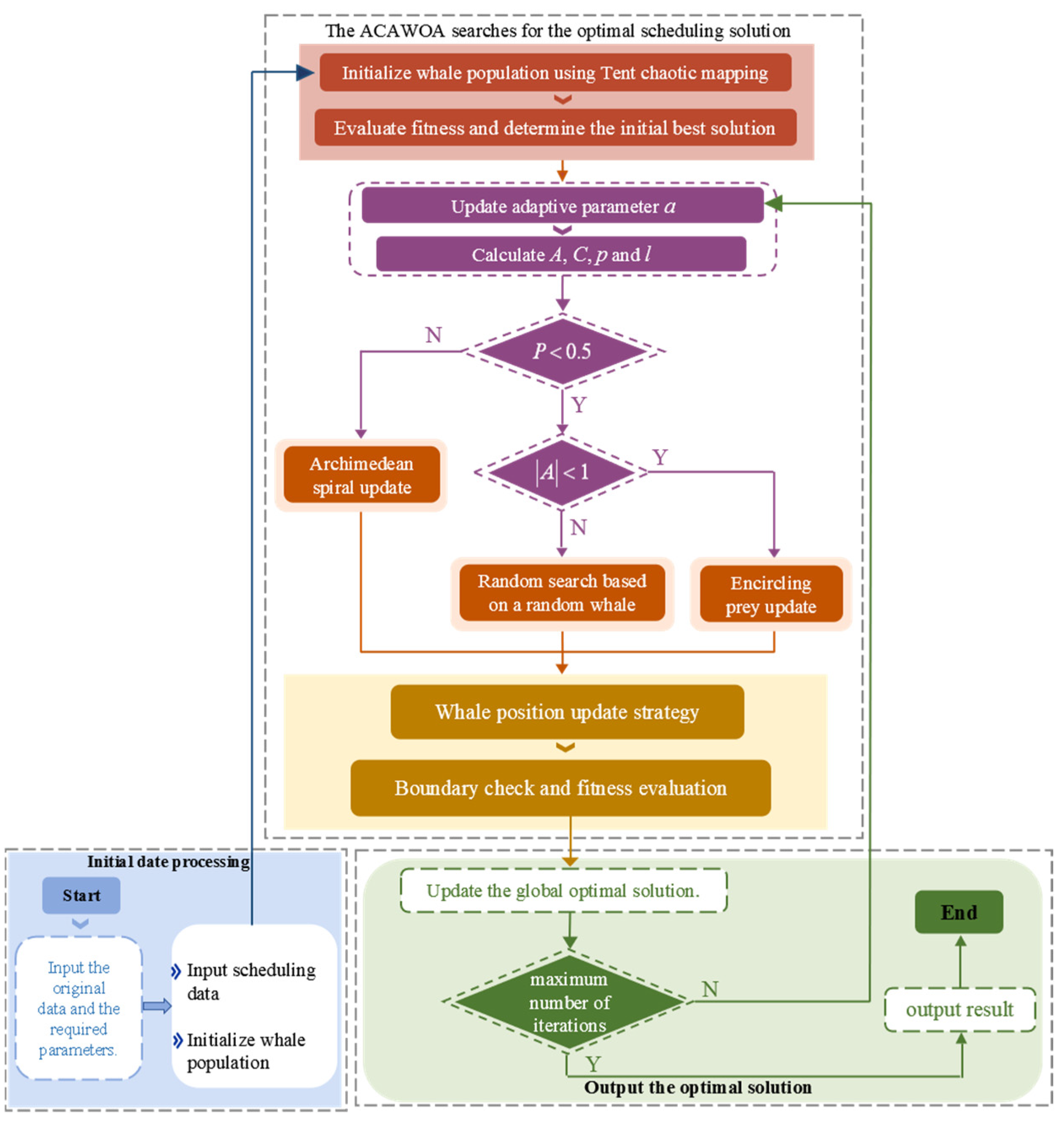
As shown in Figure 2, the proposed ACAWOA incorporates Tent chaotic initialization, adaptive parameter regulation, and Archimedean spiral search into the whale position update process, thereby improving the balance between global exploration and local exploitation.

3. Stochastic Optimization and Control Strategy for Microgrids Considering Uncertainty Factors

Microgrids inherently involve multiple uncertainty factors. Conventional microgrid optimal scheduling methods fail to account for the impacts of prediction errors and stochastic factors during the control process, thereby significantly undermining the performance of microgrid energy optimization and control.

In this paper, the uncertainty factors inherent in microgrids are fully considered. Probability functions are employed to characterize the relevant variables of microgrids, and a stochastic optimization model for microgrids is established. Based on Monte Carlo sampling with the Latin hypercube method, the uncertain optimization problem is transformed into a deterministic one for solution, and the effectiveness of the proposed method is verified through a numerical case study.

3.1. Analysis of Uncertainty Factors in Microgrids

(1)

Probability Model for Photovoltaic Power Generation

PV power generation efficiency is strongly affected by dynamic factors such as solar irradiance and ambient temperature. To quantify this uncertainty, the output is modeled using a beta distribution, with the probability density function given by the following:

$$f\left(E\right)={\displaystyle \frac{\Gamma \left(\alpha +\beta \right)}{\Gamma \left(\alpha \right)\Gamma \left(\beta \right)}}{\left({\displaystyle \frac{E}{E_{\max }}}\right)}^{\alpha -1}{\left(1-{\displaystyle \frac{E}{E_{\max }}}\right)}^{\beta -1}$$

(19)

In the formula, $f\left(E\right)$ denotes the beta probability distribution model for photovoltaics; $\Gamma \left(\alpha \right)$ and $\Gamma \left(\beta \right)$ denote the gamma function; $\alpha$ and $\beta$ are the shape parameters of the beta distribution; and E represents the real-time irradiance.

To characterize the uncertainty of PV, the prediction error can be expressed as follows:

$$\Delta P_{pv,t}=P_{pv,t}-{\widehat{P}}_{pv,t}$$

(20)

In the formula, $\Delta P_{pv,t}$ denotes the prediction error in time period t; $P_{pv,t}$ represents the actual photovoltaic power output in time period t; and ${\widehat{P}}_{pv,t}$ stands for the predicted photovoltaic power output in time period t.

(2)

Probability Model for Wind Power Generation

The two-parameter Weibull distribution is widely used to model wind speed variability and its effect on wind power output. Its probability density function is given by the following:

$$f\left(\nu \right)={\displaystyle \frac{k}{c}}{\left({\displaystyle \frac{\nu }{c}}\right)}^{k-1}\exp \left[-{\left({\displaystyle \frac{\nu }{c}}\right)}^k\right]$$

(21)

In the formula, v represents wind speed; and k and c are the shape parameter and scale parameter of the Weibull distribution, respectively.

(3)

Probability Model for Electric Vehicle Loads

EV charging load is primarily determined by per-vehicle driving distance, which is commonly modeled as lognormally distributed. Its probability density function is given by the following:

$$f_d(x)={\displaystyle \frac{1}{d{\sigma }_d\sqrt{2\pi }}}\exp \left[{\displaystyle \frac{-{(\ln d-{\mu }_d)}^2}{2{\sigma }_d^2}}\right]$$

(22)

In the formula, d represents the driving distance of the electric vehicle (km); ${\mu }_d$ represents the expected daily driving distance of the electric vehicle, ${\mu }_d=3.2$; and ${\sigma }_d$ represents the variance of the daily driving distance of the electric vehicle, ${\sigma }_d=0.88$.

The energy demand model of EV is as follows:

$$W={\displaystyle \frac{D}{S}}E$$

(23)

$$t={\displaystyle \frac{W}{P\ast \eta }}$$

(24)

In the formula, D represents the daily driving distance of the electric vehicle, measured in kilometers; S is the rated driving range of the electric vehicle, set at 300 km; E is the battery capacity of the electric vehicle, set at 62 kW·h; t is the charging time; W is the amount of electricity required to fully charge the vehicle; P is the charging power, set at 5 kW; and η is the charging efficiency, set at 0.9.

(4)

Probability Model for Conventional Loads

Active and reactive power at each system node follow a normal distribution over a given time horizon. A constant power factor model is adopted, and the probability density function of active power is given by the following:

$$f\left(P_L\right)={\displaystyle \frac{1}{\sqrt{2\pi }{\sigma }_L}}\exp \left[-{\displaystyle \frac{{\left(P_L-{\mu }_L\right)}^2}{2{\sigma }_L^2}}\right]$$

(25)

In the formula, ${\mu }_L$ and ${\sigma }_L$ represent the average and standard deviation of the power demand at various points in the distribution network, respectively.

The load demand power prediction error during the dispatch interval is given by the following:

$$\Delta P_{L,t}=P_{L,t}-{\widehat{P}}_{L,t}$$

(26)

In the formula, $\Delta P_{L,t}$ is the load power prediction error in period t, $P_{L,t}$ is the actual load power in period t, and ${\widehat{P}}_{L,t}$ is the predicted load demand power in period t.

3.2. Stochastic Optimization Model Considering Uncertainty Factors

A chance-constrained stochastic model predictive control framework is adopted for optimal scheduling. The objective is to minimize the total operating cost, given by the following:

$$\min C_{MG}=C_M+C_E$$

(27)

In the formula, $C_{MG}$ is the operating cost, $C_M$ is the operation and maintenance cost, and $C_E$ is the interaction cost with the power grid.

$$C_M={\displaystyle \sum _{t=t_0}^{t_0+T}\left(C_M^{PV}{\overline{P}}_t^{PV}+C_M^{WT}{\overline{P}}_t^{WT}+C_M^{ESS}{P}_t^{ESS}\right)}$$

(28)

In the formula, $t_0$ represents the start time of the stochastic optimization scheduling; T is the scheduling period, usually set at 24 h; $C_M^{PV},C_M^{WT},C_M^{ESS}$ represent the unit maintenance cost of photovoltaic, wind turbines and energy storage; and $P_t^{PV},P_t^{WT},P_t^{ESS}$ represent the output power at the predicted time.

$$C_E={\displaystyle \sum _{t=t_0}^{t_0+T}\left(P_{buy}^{grid}{\overline{P}}_t^{grid.b}-P_{sell}^{grid}{\overline{P}}_t^{grid.s}\right)}$$

(29)

In the formula, $P_{buy}^{grid}$ represents the purchase price of electricity; $P_{sell}^{grid}$ represents the sale price of electricity; $P_t^{grid.b}$ represents the purchase volume of electricity; and $P_t^{grid.s}$ represents the sale volume of electricity.

In microgrid optimal scheduling, spinning reserve is reserved to compensate for prediction errors, yielding the following internal power output constraint:

$${\overline{P}}_{WT}+{\overline{\epsilon }}_{WT}+{\overline{P}}_{PV}+{\overline{\epsilon }}_{PV}+{\overline{P}}_{grid}\ge {\overline{P}}_L+P_{ESS}+{\overline{P}}_{EV}$$

(30)

In the formula, ${\overline{P}}_{WT}$ represents the power of the wind turbine; ${\overline{P}}_{PV}$ represents the photovoltaic power; ${\overline{P}}_{grid}$ represents the interactive power; $\overline{P}$ represents the load demand; $P_{ESS}$ represents the charging and discharging power of energy storage; ${\overline{P}}_{EV}$ represents the power of EV; ${\overline{\epsilon }}_{WT}$ represents the prediction error of the wind turbine; and ${\overline{\epsilon }}_{PV}$ represents the prediction error of photovoltaic.

To ensure uncertain variables remain within a controllable range, Equation (30) is reformulated as a probabilistic constraint, yielding the chance constraint as follows:

$$\mathrm{Pr}\{{\overline{P}}_{WT}+{\overline{\epsilon }}_{WT}+{\overline{P}}_{PV}+{\overline{\epsilon }}_{PV}+{\overline{P}}_{grid}\ge {\overline{P}}_L+P_{ESS}+{\overline{P}}_{EV}\}\ge 1-\alpha$$

(31)

3.3. Deterministic Reformulation of Chance-Constrained Programming via Latin Hypercube Sampling

Using Latin hypercube sampling, the random variables in the probabilistic constraint are drawn $N_{\mathrm{sample}}$ times. Binary indicator variables encode constraint satisfaction for each scenario; the chance constraint is thus reformulated deterministically by requiring that at least a fraction $\alpha$ of samples satisfy the constraint, yielding the following:

$${\displaystyle \frac{1}{N_{\mathrm{sample}}}}{\displaystyle \sum _{sa=1}^{N_{\mathrm{sample}}}{d}_{sa}}\ge \alpha$$

(32)

To capture the combined effect of photovoltaic and load forecasting errors on power balance, sample errors are sorted, and the critical subset satisfying the confidence level is selected to formulate deterministic constraints:

$$\begin{array}{l}{\overline{P}}_{WT}+P_{ESS}+P_t^{grid.b}-{\overline{P}}_{PV}-{\overline{\epsilon }}_{PV}-{\overline{\epsilon }}_{WT}-P_t^{grid.s}\le \\ {\epsilon }_{WT}(ceil(N_{sample}\times \alpha ))-{\epsilon }_{PV}(ceil(N_{sample}\times \alpha ))\le 0\\ {\epsilon }_{WT}=sort\left(\left[{\overline{P}}_{WT}(1),{\overline{P}}_{WT}(2),\dots ,{\overline{P}}_{WT}(sa)\right]\right)\\ {\mathrm{e}}_{PV}=sort\left(\left[{\overline{P}}_{PV}(1),{\overline{P}}_{PV}(2),\dots ,{\overline{P}}_{PV}(sa)\right]\right)\end{array}$$

(33)

In the formula, the function of $ceil(\ast )$ is to find the smallest integer not less than the value within the parentheses, and the function of $sort\left(\ast \right)$ is to sort the phasors within the parentheses in ascending order. Thus far, the chance constraints in the original stochastic optimization model have been equivalently converted into deterministic linear constraints.

A sensitivity analysis examines how the Latin hypercube sampling sample size affects total dispatch cost and computational performance. The results are summarized in

Table 1. Sensitivity analysis of LHS sample size.

Sample Size	Cost (Yuan)	Convergence Iterations
50	41,200	150
100	40,580	165
200	40,169	170
500	40,120	185

. The results indicate that increasing the number of samples improves the accuracy and stability of the deterministic approximation of chance constraints. However, larger sample sizes also lead to increased computational burden and longer convergence times. When the sample size is small, uncertainty is insufficiently captured, which may result in suboptimal decisions. As the sample size increases, the results gradually stabilize. Beyond a certain threshold, further increasing the sample size yields only marginal improvements in cost reduction while significantly increasing computational time. Therefore, a moderate sample size is selected to balance computational efficiency and solution accuracy.

4. Case Studies Analysis

4.1. Case Study Data

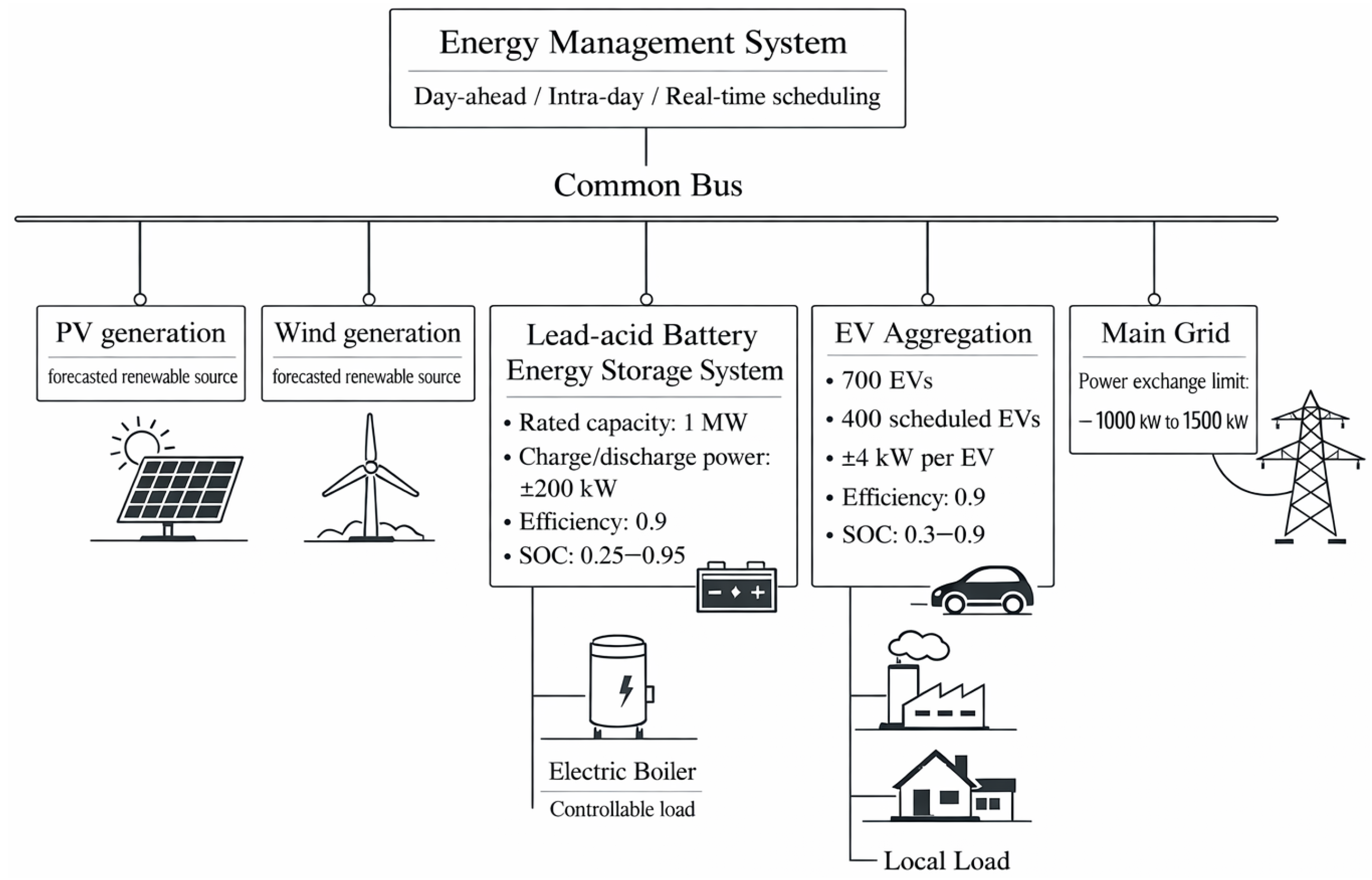
Building on this framework, a real-world microgrid in Liaoning Province is selected as the case study, and the corresponding load and renewable generation forecasts are used to evaluate the proposed method. The studied system consists of renewable generation units, an energy storage system, electric vehicles, controllable loads, local demand, and the main grid. Specifically, it includes 700 electric vehicles, among which 400 are scheduled across multiple time scales, and a 1 MW lead-acid battery energy storage system, which is adopted for modeling simplicity and compatibility with conventional microgrids; however, the framework can be extended to lithium-ion batteries by incorporating degradation mechanisms, SOH dynamics, and efficiency variations. The maximum charging/discharging power of the energy storage system is 200 kW, and the power exchange limit with the main grid ranges from −1000 kW to 1500 kW. The corresponding system configuration is illustrated in Figure 3.

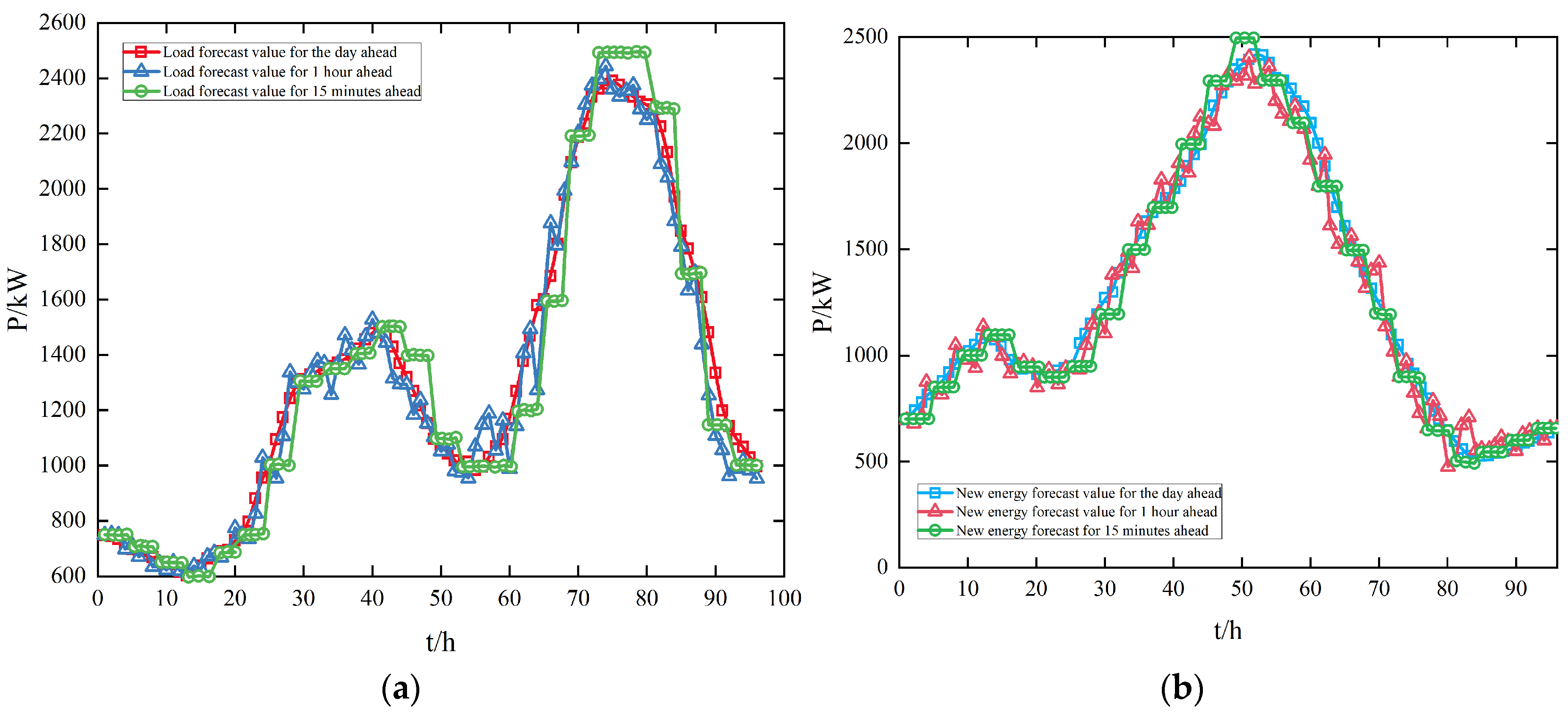
Renewable energy generation is highly volatile, introducing significant forecasting uncertainty. As shown in Figure 4, subfigure (a) presents the load forecasting curve, while subfigure (b) shows the renewable generation forecasting curve. Its day-ahead, 1 h intra-day, and 15 min intra-day power forecasts—evaluated across all hours of a day—remain within acceptable error bounds and track the real-time generation profile.

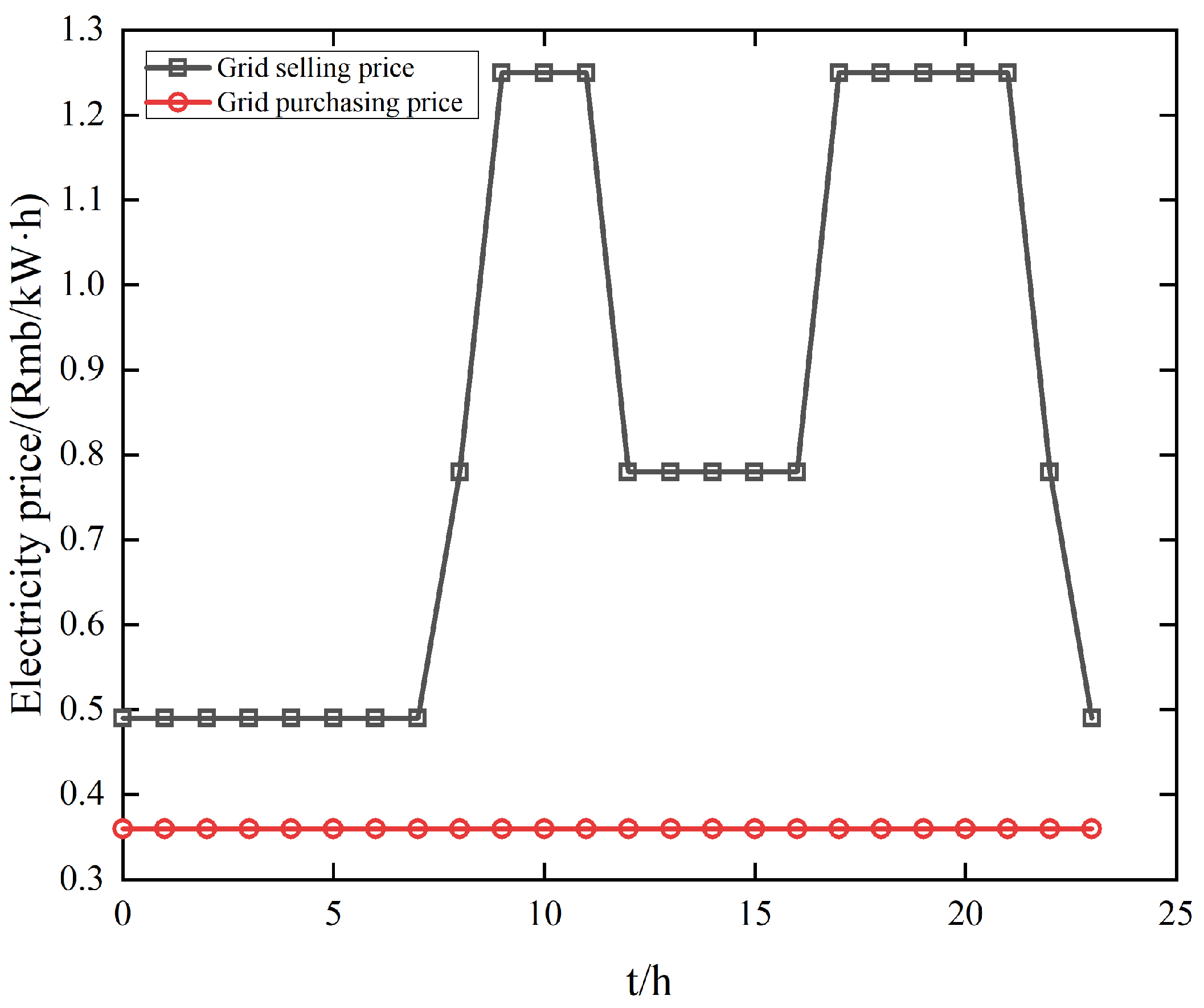
This corresponds to the day-ahead scheduling stage of the microgrid within the time-scale framework. Leveraging the principle of time-of-use tariff, the daily electricity price is categorized into peak-period, off-peak, and flat-period tariffs, with relevant price data presented in Figure 5. Operational parameters for EVs, energy storage, and the main grid are tabulated in

Table 2. Fundamental parameters of microgrid components.

Type	Maximum Output/kW	Minimum Output/kW	Discharge Efficiency	Charge Efficiency	Minimum SOC/kW	Maximum SOC/kW
EV	4	−4	0.9	0.9	0.3	0.9
energy storage	200	−200	0.9	0.9	0.25	0.95
main grid	1500	−1000

.

4.2. Analysis of Multi-Time-Scale Optimal Scheduling Results for Microgrids

(1)

Intra-Day Dispatch Results and Analysis

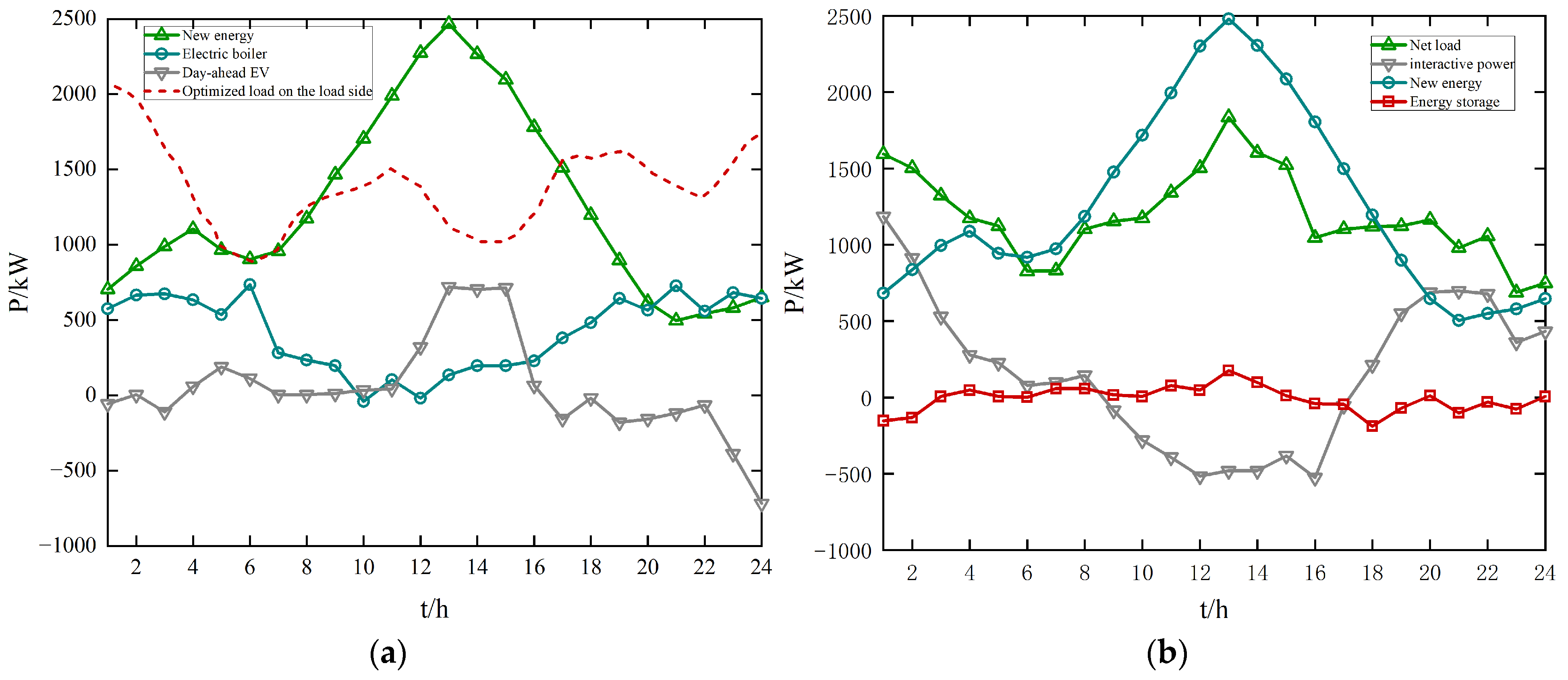
Figure 6 presents the day-ahead optimal dispatch schedule for the generation side.

Figure 6a shows the day-ahead generation-side output of EVs. The optimized load curve peaks between 00:0 and 4:00 and again after 17:00. During these periods, renewable energy sources (RESs) cannot meet grid demand. EV dispatch aligns closely with RES generation in the early connection phase, enhancing RES utilization. When RES is insufficient and time-of-use prices are high, the electric boiler supplements the supply to reduce the net load.

Figure 6b shows the bulk power grid’s generation-side output with energy storage. From 10:00 to 16:00, RE meets demand, and surplus RE is stored. After 16:00, stored energy is discharged to serve the load. After optimizing EVs, interruptible loads, and storage, the net load curves of both systems align: higher RE output correlates with higher net load, and lower RE output with lower net load. Due to storage power limits, excess RE during certain periods is curtailed and exported to the bulk grid.

(2)

Intraday Dispatch Results and Analysis

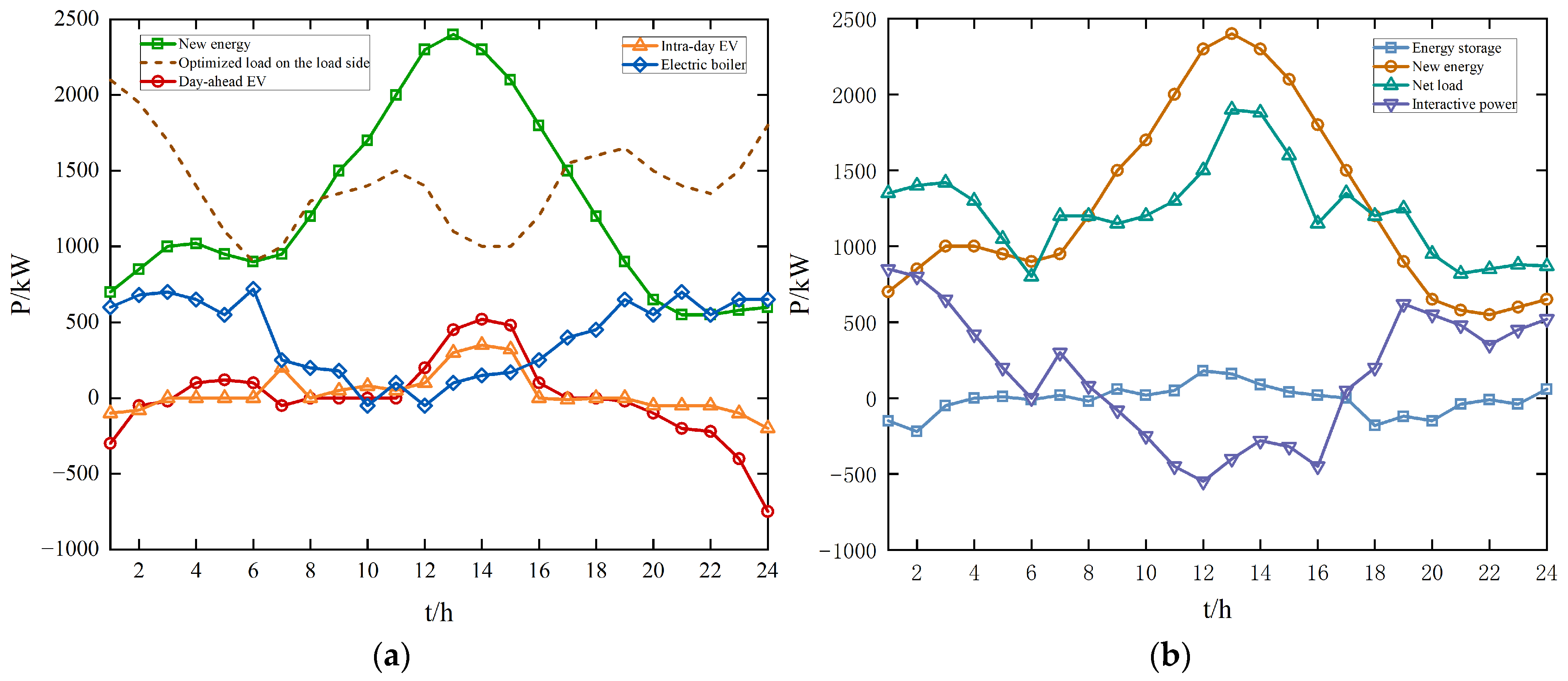
Intraday source–storage dispatch implements the day-ahead plan according to the proposed strategy. Optimal dispatch of all generation-side resources is shown in Figure 7.

Figure 7a shows the planned intraday supply-side output of EVs. From 10:00 to 16:00, EVs charge fully and modulate their power output, while RE meets load demand. After 18:00, battery storage discharges, electric boilers supply power, and non-critical loads are curtailed to compensate for the RE shortfall. EV dispatch closely follows the aggregate RE generation profile, and coordinated EV power station output improves RE utilization.

The dispatch profile of energy storage and the bulk power grid on the generation side is illustrated in Figure 7b. From 10:00 to 16:00, energy storage charges to absorb surplus RE, while discharging during nighttime to support load demand. The system’s aggregate load curve is constructed from unplanned loads, EVs, electric boilers, daily EV energy, and stored energy. Daily system optimization aligns the aggregate load curve with the RE power profile, demonstrating that optimized generation-side resource dispatch effectively enhances RE accommodation.

(3)

Real-Time Dispatch Results and Analysis

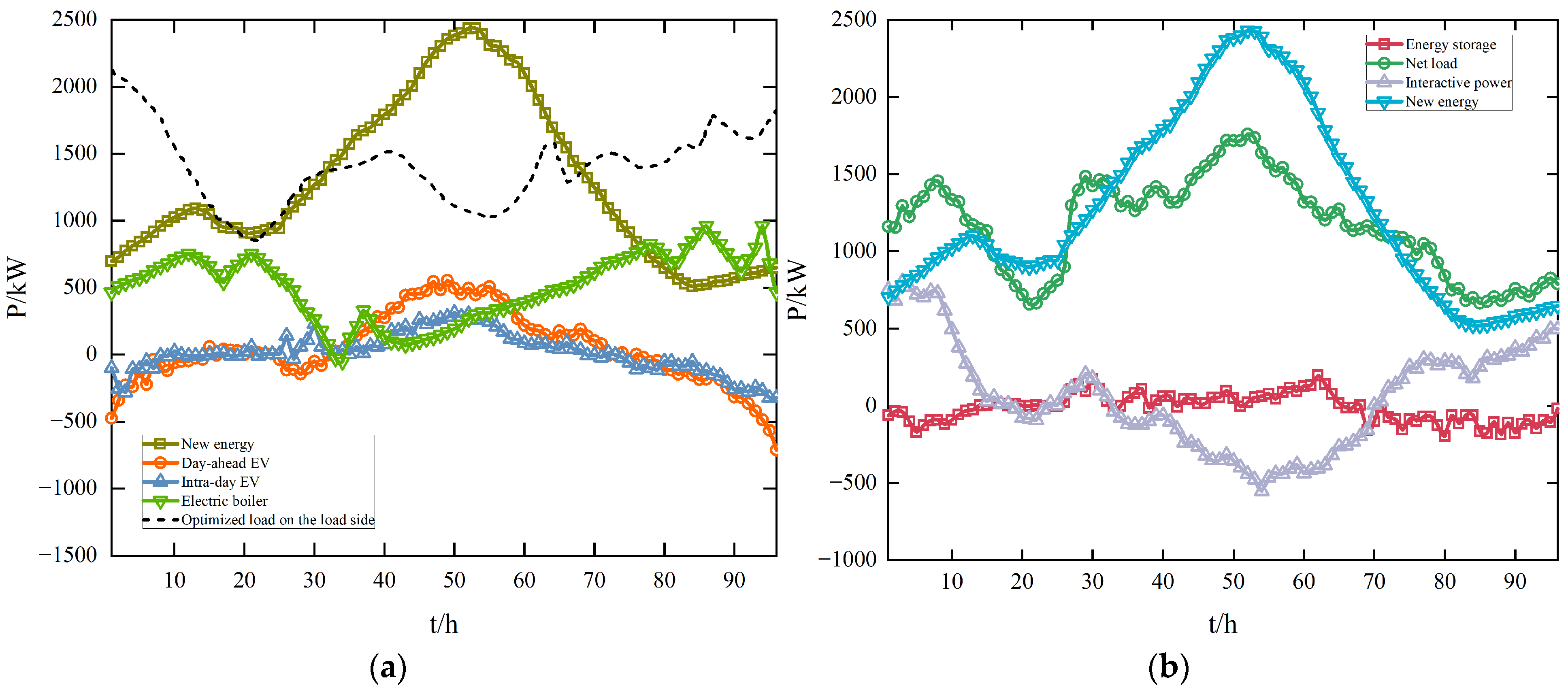
Real-time dispatch is performed on the power supply side, with continuous optimization implemented based on the intraday schedule. A 24 h optimization was conducted under the real-time dispatch mode, and the results are presented in Figure 8.

Figure 8 shows grid-side output power and load dynamics under real-time supply-side dispatch. Within key intervals, output power closely tracks the intraday schedule—exhibiting low deviation and high stability. By coordinating multi-time-scale resources, the approach maximizes RE accommodation while jointly satisfying reliability and economic objectives.

4.3. Stochastic Optimization and Control Analysis of Microgrids

To validate the proposed strategy, we conducted a stochastic optimal dispatch simulation of the microgrid. The system comprises energy storage systems, DG units, EV charging stations, and electric boilers, each occupying different nodes to form a unified power network. The simulation parameters are summarized in

Table 3. Microgrid simulation parameters.

Parameter Name	Parameter Value
$P_n^{\max }$	500 kW,
$A_{ESS},B_{ESS}$	0.01, 0.02
$A_{EB},B_{EB}$	0.008, 0.1
$P_{EB}^{\max },P_{EB}^{\min }$	50 kW, 0
$Y_{EB}^{\max }$	250 kW
${\mathrm{E}}_{\max },{\eta }_e$	50 kW, 0.9
$S_n^{\max },S_n^{\min }$	180 kW·h, 20 kW·h

.

The experimental design in this section compares the classical deterministic optimization strategy with the innovative stochastic optimization technique proposed in this chapter for optimizing the microgrid pre-scheduling scheme, aiming to validate the superiority of the novel method.

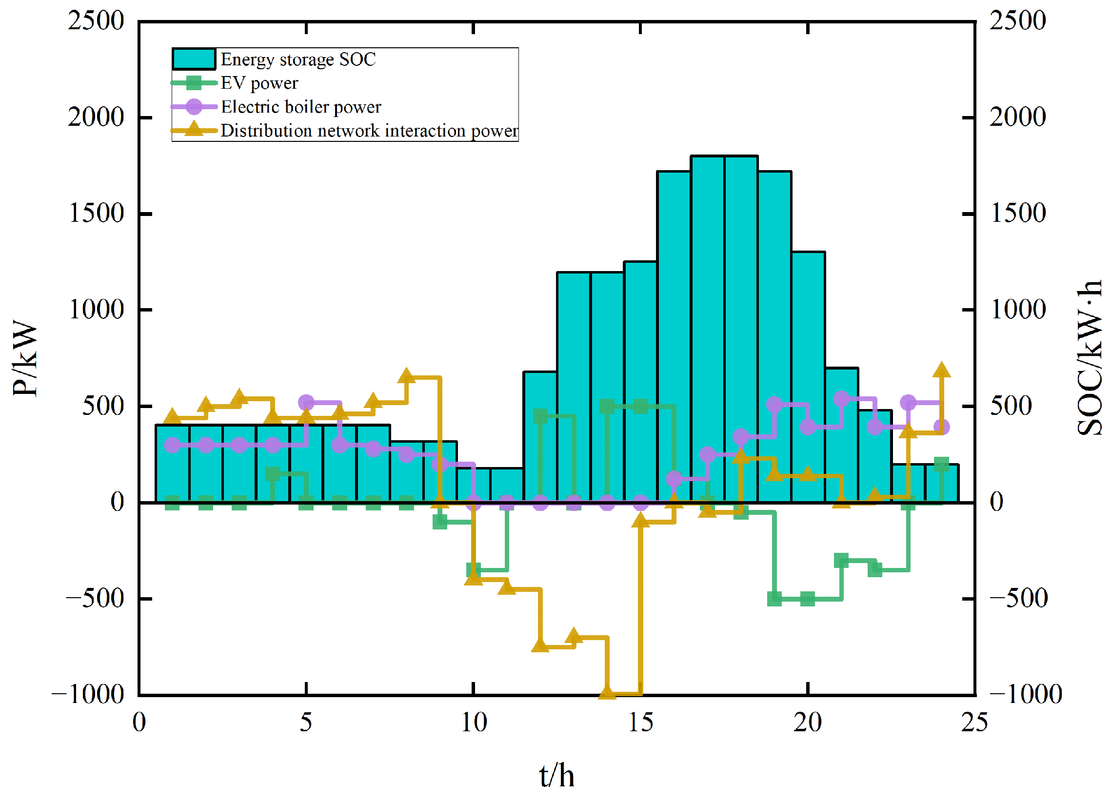
As shown in the output curve of the random optimization scheduling in Figure 9, it can be seen that from 0:00 to 7:00, since the photovoltaic system is unable to supply power, the microgrid purchases electricity from the external grid to meet the load demand, and the energy storage device maintains a zero charge and discharge power. From 7:00 to 9:00, as the photovoltaic power generation gradually increases, the load demand also increases. The random scheduling strategy determines that the microgrid’s power supply is insufficient, and the electricity price begins to rise, so the energy storage device starts discharging to reduce the cost of purchasing electricity. From 9:00 to 15:00, with a sufficient photovoltaic power supply and a decrease in load demand, the microgrid, in pursuit of economic benefits, chooses to sell electricity to the external grid, while EVs are charged, promoting local consumption of photovoltaic power. From 15:00 to 17:00, photovoltaic power generation weakens and the load increases. The energy storage device stops charging after reaching its maximum capacity. After 17:00, as the photovoltaic power supply gradually disappears and the load enters the evening peak, the energy storage device discharges to fill the power shortage. At the same time, the electric boiler operates during this period to compensate for the power deficiency of the microgrid. In summary, through such pre-scheduling, the microgrid has skillfully configured its internal resources. By flexibly using the energy storage device, it has successfully smoothed out the fluctuations in supply and demand, ensuring power balance throughout the entire operation cycle.

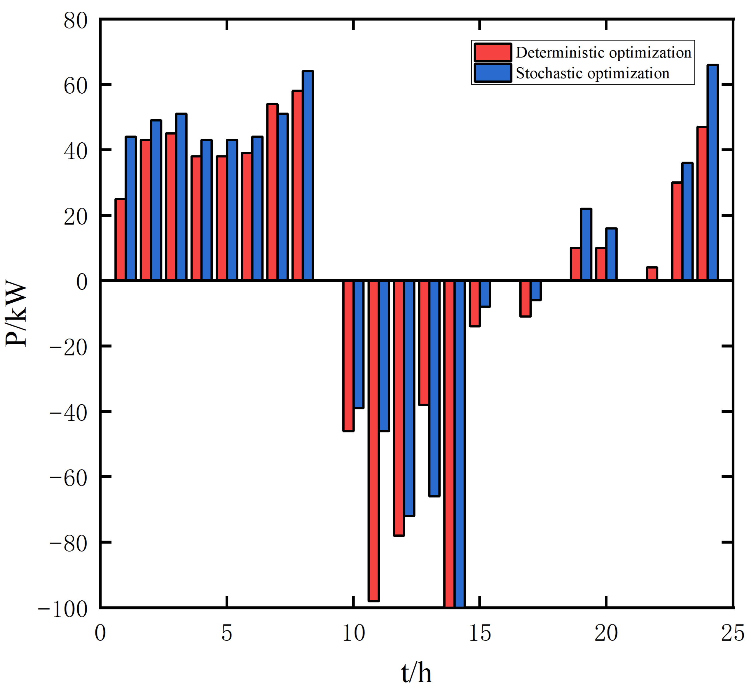
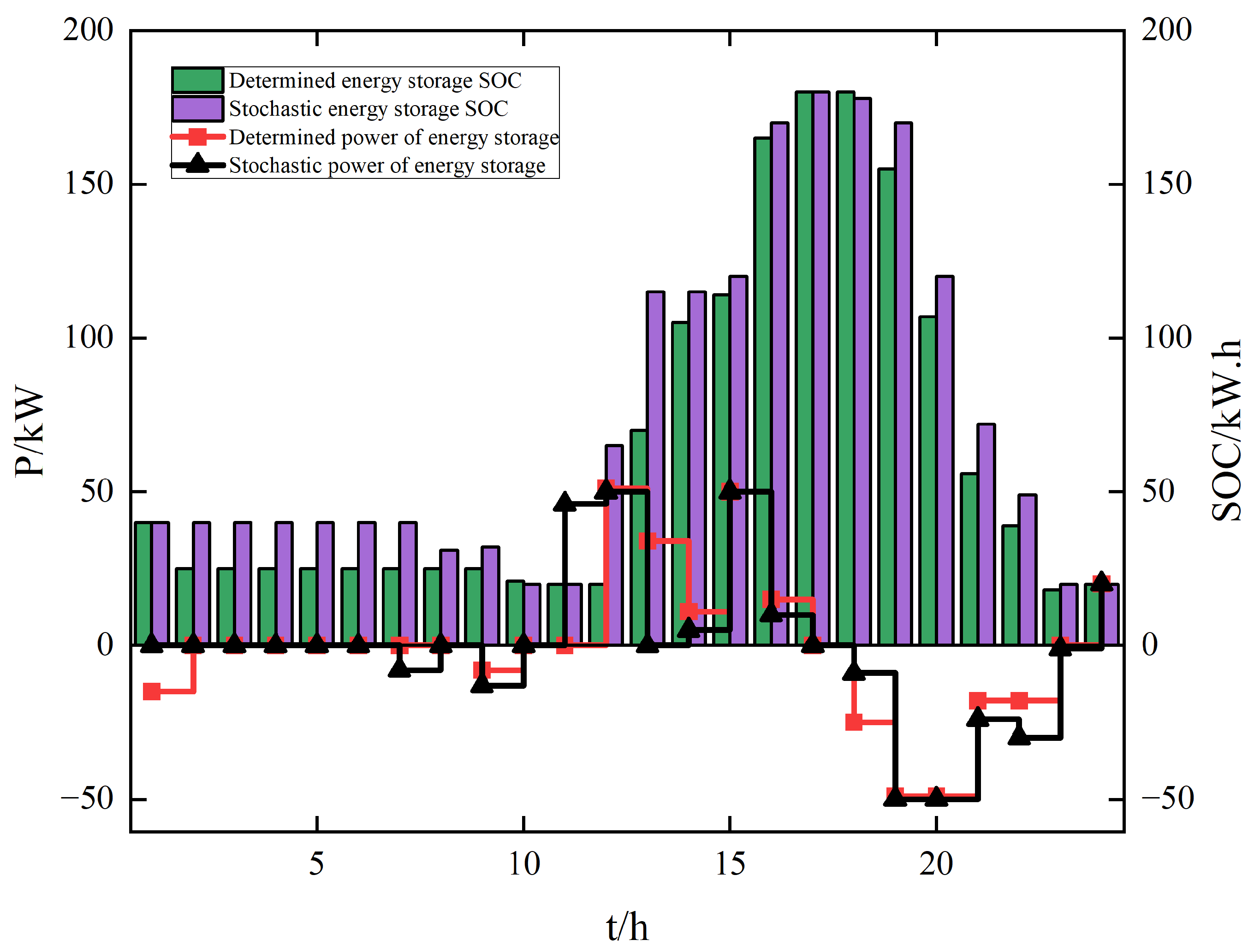
Figure 10 and Figure 11 compare the microgrid–grid interaction power and energy storage dispatch profiles of the deterministic optimal dispatch and the proposed stochastic method.

The results in Figure 10 show that the proposed strategy and deterministic optimal dispatch exhibit similar power conversion trajectories. However, by incorporating uncertainties in PV and load forecasting, the proposed method intentionally retains operational flexibility. In dispatch decisions, it prioritizes increased main grid power purchases to ensure internal power stability and enhance system adaptability.

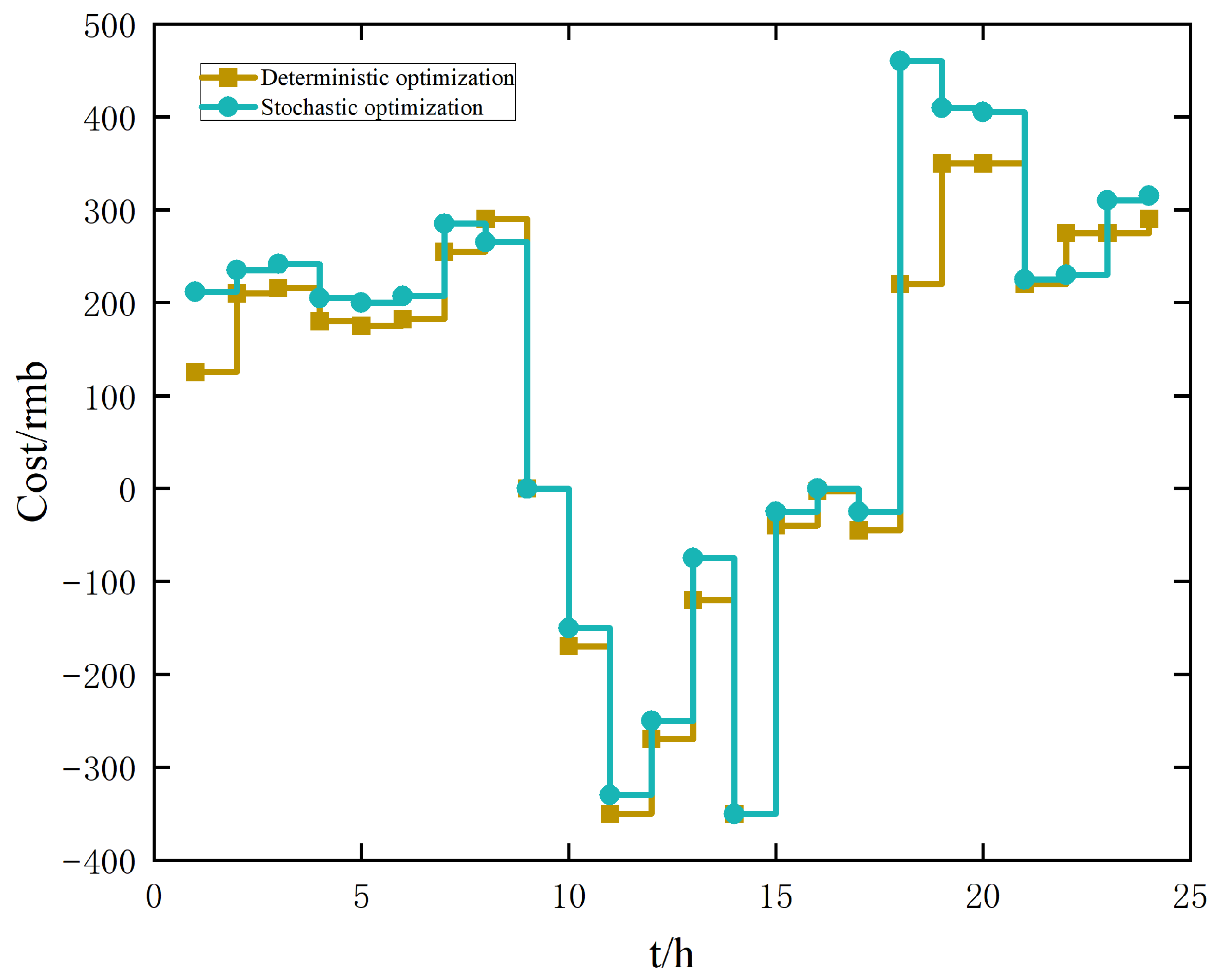
Figure 12 compares the time-resolved day-ahead operational costs of the microgrid under deterministic optimal dispatch and the proposed stochastic dispatch. The stochastic approach incurs a marginally higher total cost.

Table 4. Total day-ahead dispatch cost.

Method	Cost (Yuan)
Deterministic Optimization	42,701
Stochastic Optimization	49,736

summarizes the total day-ahead dispatch costs of the two methods.

The data in Table 4 reveal that the total day-ahead dispatch cost of the proposed stochastic optimization algorithm is marginally higher than that of the deterministic strategy. This cost increment stems from the explicit incorporation of PV power and load demand volatility, as well as their forecast errors, into the planning framework, where flexible reserve capacity is reserved to enhance the system’s robustness against uncertainty. While the cost increases, this reflects a more conservative and reliability-oriented scheduling strategy that improves the system’s ability to accommodate fluctuations in renewable generation and load demand. Given the inherent intraday variability of PV and load, the proposed method enhances the robustness and adaptability of microgrid operation under uncertain conditions. Thus, the dispatch scheme provides a more reliable basis for real-time operation, balancing economic efficiency and operational flexibility.

4.4. Algorithm Comparison

To ensure a fair and reproducible comparison, all algorithms are implemented under identical settings, with a population size of 30 and a maximum of 200 iterations. For WOA and GWO, the parameter a decreases linearly from 2 to 0, with b = 1 for WOA. In PSO, c₁ = c₂ = 2 and w = 0.7. The proposed ACAWOA incorporates adaptive parameter control, tent chaotic initialization, and an Archimedean spiral strategy. These settings follow commonly used configurations in the literature and ensure fairness and reproducibility.

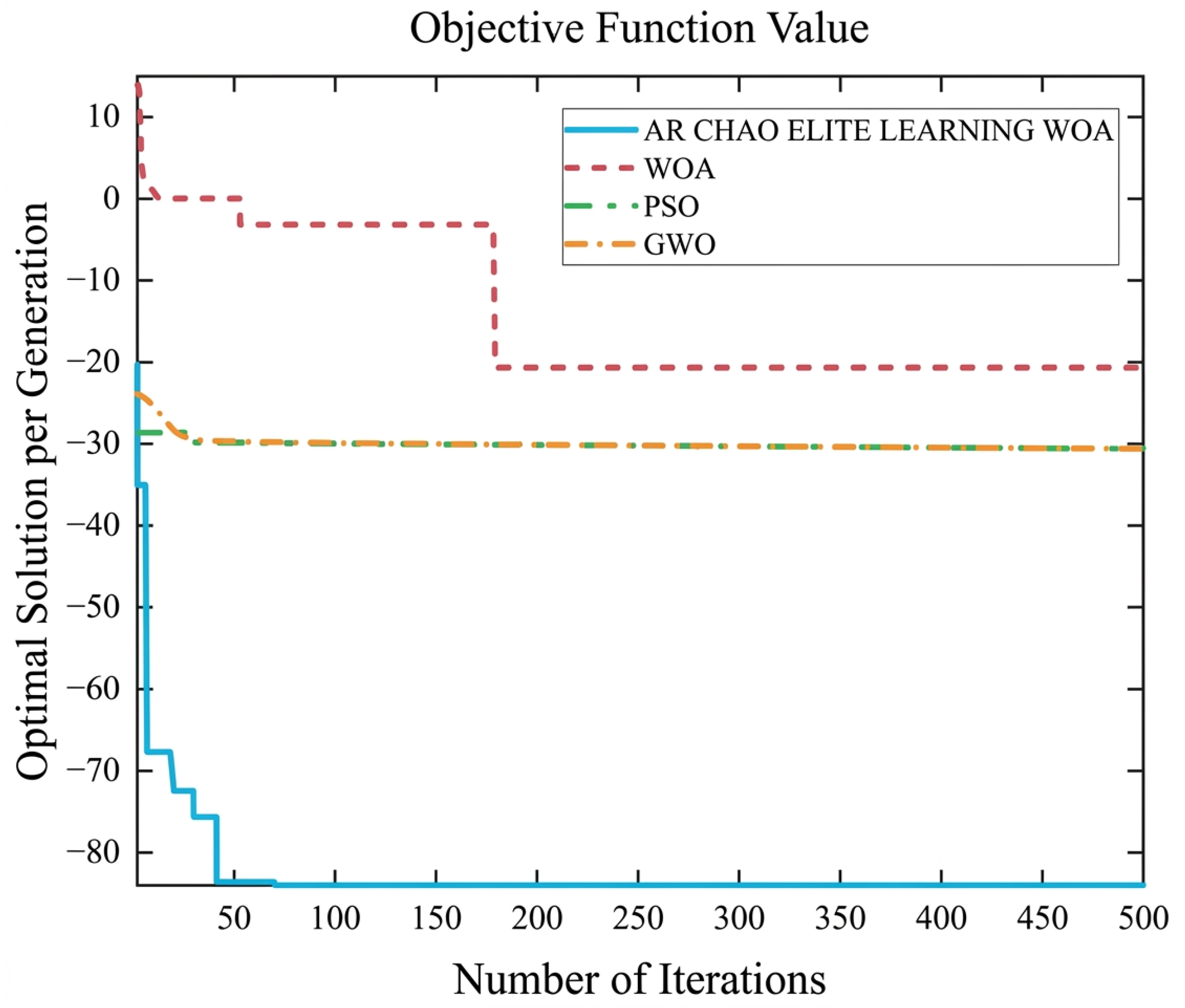
Figure 13 shows the microgrid optimization results at the 12th hour. Under abundant solar irradiance over this period, the grid-connected operation triggers substantial energy exchange with the main grid and energy storage systems. Using the “whale” method for initial random selection results in a relatively large objective function value, which exerts a non-negligible impact on the convergence rate. In contrast, the uniform DG by the tent map ensures the initial population is evenly dispersed across the solution space, thereby accelerating the optimal solution search process. To facilitate a clearer comparison of convergence behavior, the objective function values shown in Figure 13 are transformed, where the original cost values are normalized and shifted to a comparable scale; therefore, the negative values do not represent the actual operational cost, but rather a relative performance metric.

Extensive simulations show that WOA performs poorly on this problem, frequently converging to local optima. Even when escape occurs, its solution quality remains inferior to that of other benchmark algorithms. Moreover, WOA stagnates after 200 iterations—no further improvement is observed.

Notably, both the PSO and GWO also suffer from local optima during iterative processes. Both algorithms exhibit poor search performance: they are highly prone to local optima trapping, and their optimal solutions are rarely updated throughout the entire optimization process.

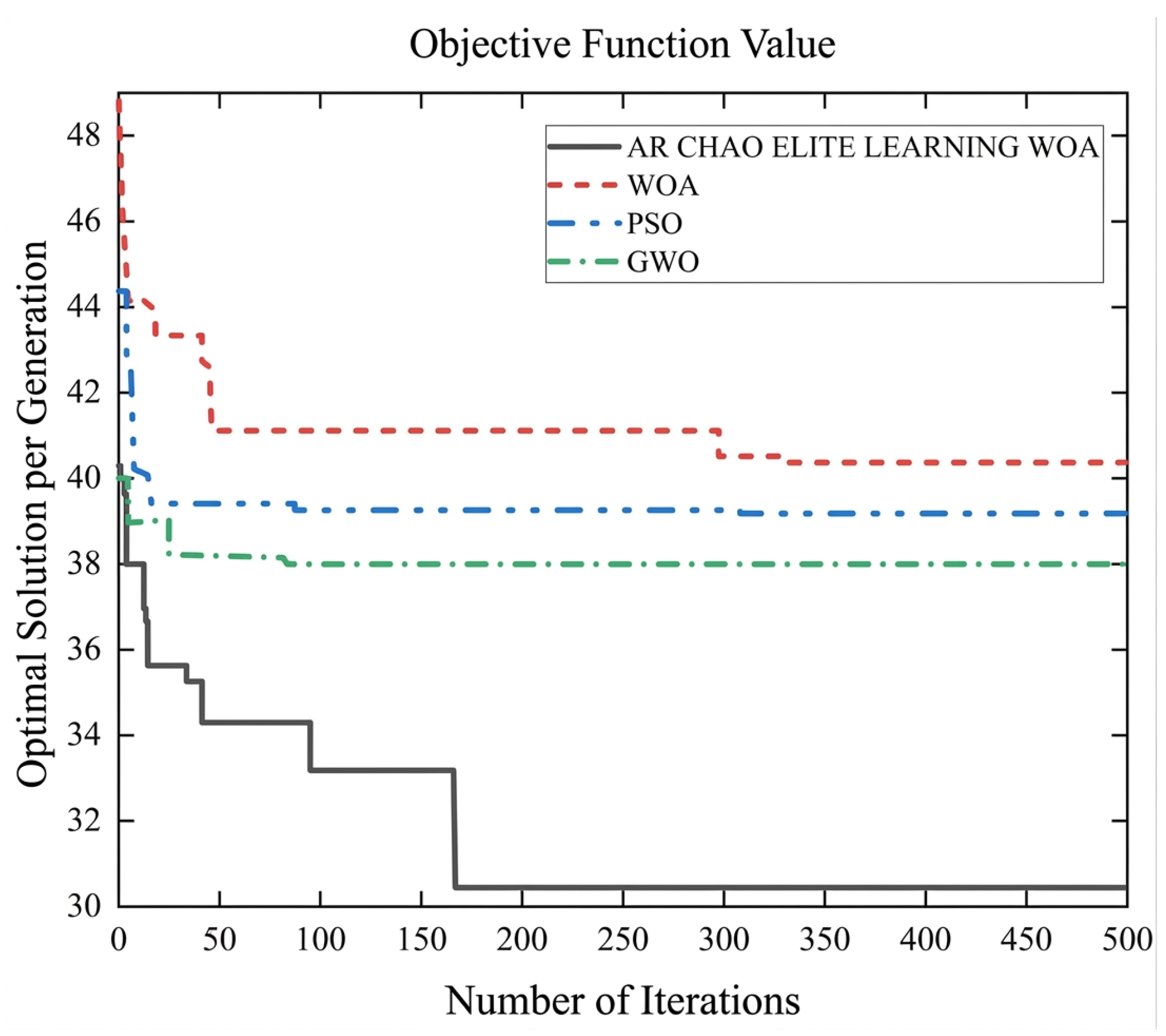
The Archimedean chaotic adaptive whale optimization algorithm (ACAWOA), enhanced by the tent map, achieves a lower initial objective function value than conventional random initialization and demonstrates strong early-stage exploration—accelerating global optimization. By incorporating the Archimedean spiral model, ACAOW improves local search efficiency and rapidly identifies the contraction direction when initialized with high-quality solutions. As shown in Figure 14, abundant photovoltaic generation at the 12th hour enables surplus energy after load satisfaction; ACAWOA leverages this to optimally charge the energy storage unit, building reserve capacity for optimal dispatch in the next hour—reducing grid reliance and improving energy efficiency.

After 24 h of optimization, WOA still failed to converge satisfactorily: its low-quality initial population resulted in poor performance and minimal solution updates. Although GWO outperformed both WOA and PSO, it suffered from limited global exploration and stagnated after 100 iterations. In contrast, the Archimedean chaotic ACAOW matched GWO’s initial population quality but achieved superior local search—rapidly identifying the contraction direction and escaping local optima even under poor initialization. ACAWOA converged to the global optimum within 170 generations, significantly outperforming standard WOA in convergence speed.

Results show that ACAWOA achieves the best objective value at convergence, escapes local optima effectively, locates the global optimum early, and converges significantly faster than all competing algorithms.

The Archimedean chaotic adaptive whale optimization algorithm optimized the 24 h power dispatch of all DERs, as shown in Figure 14. In the early morning, low PV and wind generation necessitate reliance on low-cost diesel generators to meet load demand; simultaneously, off-peak grid electricity is purchased and stored in the battery for later peak-load support. After 21:00, high PV output enables full load coverage plus surplus clean energy export for revenue—while diesel and gas turbine outputs are reduced. Although midday represents peak demand, excess clean energy is stored for contingency use. The battery’s SOC remains above the minimum operational threshold at all times, with significant surplus occurring only during peak renewable generation. Compared to mainstream swarm intelligence algorithms, ACAWOA achieves the lowest daily operational cost—demonstrating a clear economic advantage for microgrid operation.

Table 5. Comprehensive performance comparison of optimization algorithms.

Algorithm Name	Daily Optimization Cost	Std Dev	Convergence Iterations	Improvement (%)
ACAWOA	40,169	320	170	33.9%
WOA	60,782	850	200	—
GWO	48,102	620	180	20.9%
PSO	57,791	710	190	4.9%

summarizes the daily operational costs (CNY) achieved by each algorithm, where all stochastic optimization algorithms are independently executed 10 times under identical conditions. The reported cost represents the best value, while the standard deviation evaluates solution stability. WOA yields the highest cost (60,782 CNY), followed by PSO (57,791 CNY). GWO performs better with 48,102 CNY, while the proposed ACAWOA achieves the lowest cost of 40,169 CNY. Moreover, ACAWOA converges faster and provides higher solution accuracy than the other algorithms.

5. Conclusions

This study focuses on the dynamic characteristics of distributed power sources, particularly their volatility and unpredictability, and explores and applies multi-time scale analysis and random variable uncertainty processing methods to deeply optimize the energy dispatch of microgrids. A novel multi-time-scale strategy and a stochastic-resilient dispatch model are proposed, with the dual objectives of enhancing microgrid stability and economic efficiency. The key contributions of this work are outlined as follows:

(1)

A multi-time-scale scheduling framework is proposed for efficient microgrid operation—covering day-ahead, intra-day, and real-time stages. A deterministic–stochastic hybrid model jointly minimizes operational cost and maximizes renewable utilization by integrating load and renewable forecasts with day-ahead electricity prices. DERs are optimized in the day-ahead stage via a unified objective. Intra-day and real-time adjustments correct forecast errors dynamically, enabling responsive dispatch and improved performance. Coordinated control of EVs, electric heaters, and storage ensures precise load balancing and continuous calibration of net load and grid power. Experiments validate the framework’s effectiveness and robustness.

(2)

The classical WOA is critically analyzed and found to suffer from premature convergence and weak local search. To address these, we propose an Archimedean chaotic adaptive WOA: tent mapping diversifies the initial population for stronger global exploration; adaptive parameter control balances exploration and exploitation; and the Archimedean spiral improves local search precision. Comparative experiments on microgrid optimization—against WOA, PSO, and GWO—show ACAWOA achieves higher solution accuracy, faster convergence, and greater robustness.

(3)

A novel stochastic optimal dispatch model is proposed, explicitly accounting for uncertainties from wind/solar generation, EV demand, and forecast errors. Uncertainty models for microgrid random variables are formulated, and chance constraints are reformulated as deterministic equivalents to transform the stochastic optimization problem into a solvable mixed-integer programming problem. Results indicate that while day-ahead stochastic optimization incurs a marginal increase in dispatch cost, it enhances the robustness and adaptability of the system under uncertainty. This approach provides an effective framework for capturing the stochastic characteristics of renewable generation and load demand, while satisfying the dual objectives of microgrid economy and operational reliability.

Although the proposed method improves the economic efficiency and robustness of microgrid operation, it still has limitations in representing complex practical scenarios. Therefore, future research will enhance its applicability by incorporating vehicle-to-grid (V2G) degradation costs for more accurate EV modeling, validating the strategy through hardware-in-the-loop (HIL) experiments, and investigating the impact of extreme weather conditions on renewable uncertainty and system performance to further improve the robustness of the stochastic optimization model.