Decoding the Energy-Economy-Carbon Nexus: A TFT-ASTGCN Deep Learning Approach for Spatiotemporal Carbon Forecasting in the Yellow River Basin, China

Abstract

This study systematically examines the low-carbon transition challenges faced by the Yellow River Basin, a core strategic energy base in China with a coal-dominated energy system, under the dual carbon goals. Existing studies based on traditional econometric models or single-province analyses are mostly limited to static analysis, failing to simultaneously capture the nonlinear spatiotemporal evolution, cross-regional spillover effects, and long-term changing trends of carbon emissions in the basin. To fill this gap, this study builds an Energy–Economy–Carbon (EEC) analytical framework, and develops an integrated TFT-ASTGCN deep learning framework. Specifically, we employ the Temporal Fusion Transformer (TFT) for high-precision multivariate time-series simulation and peak forecasting, while the Attention-based Spatial–Temporal Graph Convolutional Network (ASTGCN) is used to identify complex spatial dependencies of inter-provincial emissions. The empirical results confirm that: (1) Basin carbon emissions show significant coal-driven carbon lock-in, with initial decoupling between economic growth and emissions. (2) Most provinces will maintain rising emissions under the current development mode, posing severe challenges to carbon peaking. (3) Asymmetric spatial spillover effects are prominent, underscoring cross-regional collaborative governance as a critical pathway for achieving an early and stable carbon peak in the basin.

1. Introduction

Carbon emissions represent a critical environmental challenge confronting nations worldwide in the post-industrial era. The excessive release of greenhouse gases has profoundly altered the earth’s living environment, necessitating urgent policy formulation and concrete actions to safeguard human habitability. As a typical resource-based economic region, the Yellow River Basin has long been trapped in a carbon-locked state characterized by high energy consumption, high emissions, and low efficiency, facing a structural dilemma of deep coupling between economic growth and carbon emissions. The path dependence and systemic inertia exhibited in this region resonate structurally with globally recognized industrial transition zones such as Germany’s Ruhr region and the United States’ Rust Belt, collectively revealing the universal challenges faced by high-carbon industrial areas in pursuing sustainable development. In Europe, similar structural issues have also garnered widespread attention, and related research provides important theoretical underpinnings for understanding such transition dilemmas [1,2]. Therefore, analyzing the driving mechanisms and unlocking pathways of carbon emissions in the Yellow River Basin is not only of pressing significance for overcoming the basin’s own developmental bottlenecks but also provides important theoretical reference and strategic insights for similar regions worldwide in addressing climate governance and industrial transformation. Energy consumption and economic development are primary pathways driving carbon emissions. The 2024 International Energy Agency conference emphasized accelerating the transition to clean energy, echoing the global call for sustainable green development under the Paris Agreement. Studies [3] indicate that global carbon emissions are closely linked to energy and economic activities, while the widespread adoption of electricity and renewable energy has contributed to reducing greenhouse gas emissions. To date, 195 countries, including China, and the European Union have actively participated in the United Nations Climate Change Conferences, contributing to global efforts for green and sustainable human development.

China maintains an energy self-sufficiency rate of around 80% and remains heavily reliant on traditional energy. Although clean energy has begun to develop, challenges such as insufficient transition technologies and regional supply-demand imbalances keep energy-related carbon emissions dominant. Regions like Shandong and Hebei, as major industrial hubs, rank among the highest in carbon emissions nationwide. In contrast, economically developed areas such as Zhejiang and Shanghai, which have limited traditional energy production, exhibit moderate carbon emission levels. Meanwhile, provinces like Qinghai and Hainan, which rely more on clean energy, record relatively low emissions. Overall, China’s energy resources are predominantly concentrated in the central and western regions, whereas the demand centers are located in the east. Economically, the northeast focuses on revitalization, the west on development, the central region on growth, and the east on modernization. Spatially, carbon emissions display a pattern of being lower in the south and higher in the north.

China has played a significant role in global environmental protection and carbon reduction, committing to reducing carbon emissions by 2030 and achieving carbon neutrality by 2060, supported by a dual-control system that systematically plans its carbon emission framework to facilitate these goals. As the world’s largest developing nation, China continues economic growth while facing substantial energy demands, resulting in considerable total carbon emissions. Therefore, in planning its carbon emission pathways and pursuing low-carbon development, China must navigate the dual challenges of transitioning its energy system while sustaining high-quality economic growth. The energy sector, as the primary source of carbon emissions, plays a critical role in determining the success of China’s carbon peaking and carbon neutrality goals. This is particularly true given China’s status as the world’s largest producer and consumer of coal. Concurrently, economic factors such as industrial structure, pathways for industrial upgrading, and the costs of technological investments profoundly influence and shape the pace and mode of energy transition. Against this backdrop, forecasting carbon emissions in China’s Yellow River region is essential for informing policy and guiding effective energy conservation and emission reduction strategies.

Currently, many researchers have conducted in-depth research on carbon emissions and their forecasting. den Elzen et al. [4] quantified all possible net-zero target scenarios and projected carbon emissions before 2050 based on the IMAGE model, yet relying solely on a single integrated assessment model like IMAGE makes it difficult to avoid inherent technical assumption biases. Friedlingstein et al. [5] investigated net land carbon dioxide emissions by revising indicators such as land-use change emissions and lateral carbon fluxes, but their approach lacks sufficient causal characterization. Costantini et al. [6] used multiple linear regression and random forest models to predict carbon dioxide emissions in 117 countries and identified key factors explaining emission pathways, though the analysis lacked adequate spatial and temporal heterogeneity. Friedlingstein et al. [7] analyzed the impact of greenhouse gases on the Earth’s system and concluded that future warming is influenced by future emissions rather than past or current ones, yet they did not fully address missing tipping points and threshold considerations.

The main contributions of this paper are as follows: (1) While prior studies have often focused on singular dimensions in carbon emissions studies, this paper integrates both energy and economic factors into the analysis of carbon emissions to examine their interrelationships. (2) Existing studies on the spatiotemporal dynamics of carbon emissions remain insufficient, particularly regarding their linkages with energy and economic dimensions. This paper provides in-depth research into the spatiotemporal interactions between carbon emissions, energy, and the economy. (3) Current studies employing machine learning approaches predominantly rely on traditional methods such as XGBoost and Random Forest. This paper innovatively applies the TFT and ASTGCN models to investigate and forecast the spatiotemporal patterns of carbon emissions.

Based on this, the structure of this paper is as follows: Section 1 is the introduction; Section 2 provides a literature review, primarily focusing on methods relevant to this study; Section 3 introduces the relationship models among energy, economy, and carbon emissions, including the spatial durbin model and system GMM, as well as the machine learning and forecasting models, along with data sources; Section 4 presents the analysis of machine learning results, mainly covering relationship analysis, spatiotemporal changes in carbon emissions, and predictions; Section 5 summarizes the conclusions; and Section 6 is the discussion section, which includes experimental limitations and future prospects.

2. Literature

The influencing factors of carbon emissions are highly systematic, with profound linkages to energy structure and economic development patterns. Existing research has revealed this complexity from multiple perspectives: Cantone et al. [8], by constructing a weighted moving average model of carbon price expectations combined with negative binomial regression, demonstrated that reasonable carbon pricing helps curb emissions and emphasized the critical role of developing new energy and energy-saving technologies in low-carbon transitions. However, their study did not fully account for corporate heterogeneity and endogeneity issues. The long-term impact of energy infrastructure also cannot be overlooked. Dan Tong et al. [9] highlighted that existing and planned power plants could emit tens of billions of tons of carbon dioxide in the future through a lock-in effect, underscoring the climate implications of energy investment decisions. Inês Azevedo et al. [10] provided guidance for policymakers by analyzing net-zero energy systems through known factors such as energy and unknown variables like technology and policy. Kiarsi and Masoudi [11] focused on economic policy dimensions, examining the interaction mechanisms between carbon taxes and fiscal policies to balance emission reduction with economic growth. Collectively, these studies indicate that carbon emission governance requires the integrated application of multi-dimensional approaches, including price signals, technological innovation, infrastructure planning, and policy coordination.

The Spatial Durbin Model (SDM) is one of the most fundamental and widely applied models in spatial econometrics, designed to handle cross-sectional or panel data characterized by spatial dependence. Building upon the classical linear regression framework, it incorporates both the spatially lagged dependent variable and spatially lagged independent variables. Its core lies in the introduction of a spatial weight matrix, enabling a more comprehensive capture of mutual influences among variables across geographical or economic spaces. In the SDM, the spatial weight matrix and the spatial lag terms jointly define the rules of spatial association. Currently, the Spatial Durbin Model is extensively utilized in correlation analysis, with scholars employing it to examine spatial linkages among various factors. For instance, Chen and Li [12] innovatively integrated spatiotemporal dependence and distributional heterogeneity analysis using a DSDQR model, concluding that achieving carbon neutrality requires spatially coordinated governance. However, their study was constrained by the exogenous assumption of the spatial weight matrix and potential bidirectional causality among core variables, which may affect the comprehensiveness and explanatory power of the findings. Similarly, Li et al. [13] analyzed the relationship between the digital economy and carbon emissions by constructing a spatial matrix to deeply investigate spatial spillover effects across 271 prefecture-level cities. Su et al. [14] explored the link between green finance and China’s carbon emissions, concluding that green resources and concepts exhibit a spatial radiation effect. Furthermore, Wanhai You and Lv [15] employed spatial panel data analysis to examine the spillover effects of economic globalization on carbon emissions, finding that the negative indirect effects on emissions significantly outweighed the positive direct effects. With its unique advantage of simultaneously capturing spatial dependence in both dependent and independent variables, the Spatial Durbin Model has proven to be a powerful tool for uncovering complex spatial correlations and spillover effects.

System GMM is an econometric approach used to estimate dynamic panel data models. It excels at addressing endogeneity issues and time-invariant individual heterogeneity within models, and can compensate for the limitation of Difference GMM when lagged level variables exhibit weak correlation with differenced variables in cases where explanatory variables approximate a random walk. The system GMM model has been widely applied in areas such as analyzing climate policies and energy poverty [16], factors of economic growth [17], determinants of ecological well-being [18], and green production factors [19]. In summary, as a rigorous and robust econometric tool, the core value of system GMM lies in its systematic combination of information from both differenced and level equations, effectively overcoming the inherent endogeneity and individual heterogeneity problems in dynamic panel data. In this paper, the System GMM model is employed to further analyze endogeneity issues among variables, building upon the foundation of the spatial durbin model.

The Temporal Fusion Transformer (TFT) model is an advanced deep learning framework specifically designed for time series forecasting, originally proposed by Lim et al. [20]. It integrates multiple neural network mechanisms to handle complex relationships within time series data, aiming to address uncertainties and multi-scale dependencies. The TFT model excels at capturing both long-term and short-term dependencies in complex temporal data while simultaneously processing static covariates, known future inputs, and unknown time-varying features, thereby generating precise and interpretable predictions. Its notable strength lies in its ability to flexibly integrate multi-scale temporal information and, through a built-in variable selection mechanism, automatically identify the most important features for forecasting. This significantly enhances the model’s adaptability and robustness in multivariate time series scenarios. As the TFT model is relatively recent, its current applications span fields such as energy [21,22] and environmental studies [23].

Attention-based Spatial–Temporal Graph Convolutional Network (ASTGCN) is a deep learning model specifically designed for spatiotemporal sequence prediction tasks, such as traffic flow and speed forecasting. It was first introduced in 2019 at AAAI, a top-tier international conference in artificial intelligence. Its core innovation lies in organically integrating graph convolutional networks with spatiotemporal attention mechanisms within a unified framework. This design simultaneously and dynamically models the complex spatial topological dependencies and temporal dynamic patterns in traffic data, thereby significantly enhancing prediction accuracy. The key architecture of ASTGCN consists of two main components: the spatiotemporal attention module and the spatiotemporal convolution module. The spatiotemporal attention module includes spatial attention and temporal attention. The former dynamically captures the varying mutual influence intensities among different nodes in a road network, while the latter focuses on learning the dynamic correlations between different historical time steps and the target prediction moment in the time series. This design enables the model to adaptively focus on the most critical spatiotemporal information, rather than treating all inputs uniformly or statically. Although ASTGCN was initially developed for traffic prediction, its modeling philosophy has gradually been extended to other spatiotemporal sequence problems, such as electricity load forecasting [24], risk assessment [25], and numerical estimation [26].

With the deepening of research on carbon emission prediction, the methodologies have gradually evolved from traditional statistical analysis and econometric models towards paradigms of machine learning and deep learning. Scholars are not only dedicated to constructing more refined carbon emission accounting systems but also actively exploring how to utilize data-driven approaches to reveal the complex interconnections between carbon emissions and systems such as energy and economy. In terms of methodological progression, research has advanced from early predictions based on linear regression and time series analysis, to the adoption of classic machine learning models like Random Forest, Support Vector Machines, and XGBoost, and further to deep learning architectures, such as Recurrent Neural Networks, Transformers, and their variants, which are capable of handling multivariate, non-linear, and high-dimensional interactions. These methods demonstrate significant advantages in capturing the temporal dynamics, feature importance, and spatial heterogeneity of carbon emissions, providing more powerful tools for simulating carbon peaking and neutrality pathways and for policy evaluation.

Table 1. Carbon emission literature based on various machine learning models.

Author	Literature	Model
Wang et al. [27]	A deep learning framework for global transportation energy carbon emission forecasting: integrating generative pre-trained transformer with multi-scale feature analysis	TransCarbon-GPT
Zhao and Jiang [28]	The Spatiotemporal Prediction Model of Urban Carbon Emissions Based on Graph Neural Networks	GNN model
Liu et al. [29]	Carbon emissions predicting and decoupling analysis based on the PSO-ELM combined prediction model: evidence from Chongqing Municipality, China	PSO-ELM joint prediction
Begum and Mobin [30]	A machine learning approach to carbon emissions prediction of the top eleven emitters by 2030 and their prospects for meeting Paris agreement targets	Six machine learning methods including SVR, XGBoost, GradBoost and K-Nearest Neighbors
Khajavi and Rastgoo [31]	Predicting the carbon dioxide emission caused by road transport using a Random Forest (RF) model combined by Meta-Heuristic Algorithms	Random Forest (RF) model
Zhang [32]	Enhanced short-term carbon emission forecasting via hybrid decomposition-denoising modeling	CEEMDAN model
Šimić et al. [33]	Assessment of the decarbonization efficiency in the European Union: machine learning approach	RNN model

summarizes representative literature, comparing the models employed. However, existing deep learning models predominantly focus on temporal dimension modeling and often overlook the critical influence of spatial graph structures on regional carbon emission linkages and synergistic reduction. Carbon emissions not only evolve over time but also exhibit complex spatial interactions and spillover effects. This is particularly true in regions like the Yellow River Basin, where provinces are geographically adjacent and economically interconnected. Factors such as energy transfers and industrial collaboration between provinces form a dynamic spatial network that directly impacts overall emission pathways and mitigation effectiveness. Ignoring spatial structures can lead to predictions that deviate from the actual mechanisms of synergistic emission reduction, making it difficult to support precise spatial policy design. To address this, this paper achieves a dual methodological breakthrough: it introduces TFT to enhance the accuracy and interpretability of temporal predictions, and innovatively adopts the ASTGCN model to incorporate spatiotemporal graph structures into carbon emission forecasting for the Yellow River Basin for the first time. ASTGCN utilizes a dynamic spatial adjacency matrix to simultaneously capture geographic proximity, energy-economic linkages, and their time-varying interaction intensities between provinces, enabling integrated modeling of both the temporal evolution and spatial association of carbon emissions. This approach not only compensates for the shortcomings of traditional temporal models in the spatial dimension but also, by identifying asymmetric spatial influence networks, provides a structured analytical tool for deciphering regional carbon emission spillover mechanisms and designing inter-provincial synergistic emission reduction pathways. This significantly strengthens explanatory and predictive capabilities across both temporal and spatial dimensions.

3. Research on the Model

3.1. Energy–Economy–Carbon Emission Correlation Analysis Mode

To systematically uncover the complex mechanisms underlying the EEC system, this study adopts a multi-dimensional validation strategy. First, given that regional carbon emissions are not independent but are jointly influenced by geographical proximity, energy flows, and economic linkages, this study employs the SDM to capture the spatial dependence of carbon emissions and the spatial spillover effects among variables. Second, to address endogeneity issues arising from the inherent path dependence of carbon emissions and the potential bidirectional causality among energy, economy, and carbon emissions, this study further employs the system GMM approach for dynamic panel estimation. By integrating these two econometric models, this study can robustly identify the marginal impacts of core driving factors within the EEC system while controlling for both spatial interactions and endogeneity biases.

3.1.1. Variable Selection

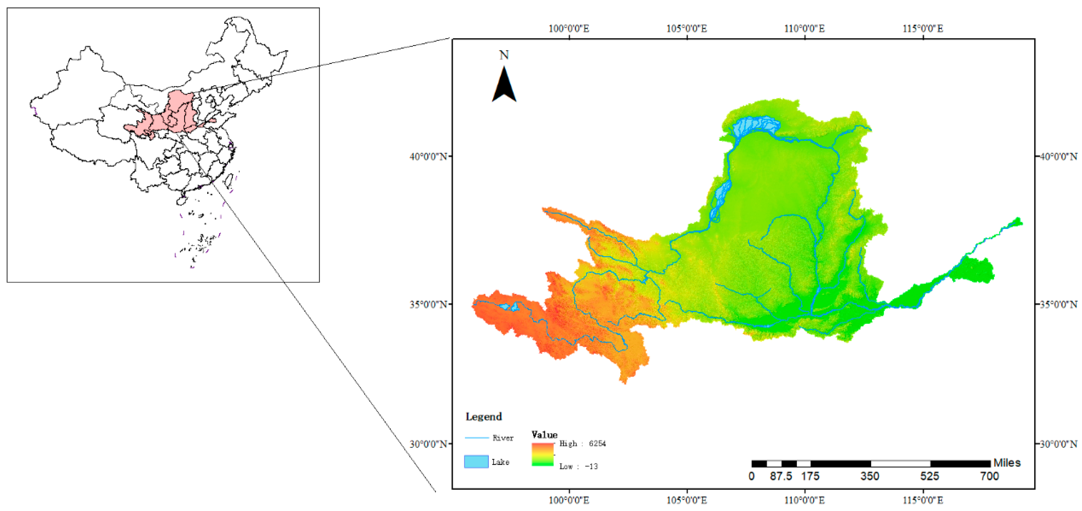
Drawing on relevant literature [34,35], this study selects energy, economy, and carbon emission-related indicators from 2005 to 2022 for the nine provinces of the Yellow River Basin, namely Qinghai, Sichuan, Gansu, Ningxia Hui Autonomous Region, Inner Mongolia Autonomous Region, Shaanxi, Shanxi, Henan, and Shandong (Figure 1), to analyze the relationships within the energy-economy-carbon emissions (EEC) system. The chosen indicators are representative, scientifically grounded, and accessible, meeting the requirements for analyzing inter-subsystem correlations. A total of 6 indicators are selected, as shown in

Table 2. Individual subsystem variables.

Subsystem	Dimensionality	Index	Unit	Serial Number	Explain
Energy	Product	Proportion of Fossil Fuel Production	%	E1	Including raw coal production, crude oil production, and natural gas production
	Consumption Scale	Total Energy Consumption	Ten thousand tons of standard coal	E2	Reflect the total regional energy demand
	Consumption Structure	Proportion of Coal Consumption	%	E3	Coal consumption/Total consumption
Economy	Economic Scale	Regional Gross Domestic Product	Hundreds of millions	J1	It reflects the total regional economic volume, and economic growth is usually accompanied by an increase in energy demand.
	Industrial Structure	Proportion of Added Value in the Secondary Industry	%	J2	Secondary industry is related to carbon emission
Carbon emission	Carbon emission scale	Total Regional Carbon Dioxide Emissions	Million tons	C1	Covers CO2 emissions in multiple areas

.

Dependent Variable is total regional carbon dioxide emissions (C1), referring to the aggregate carbon emissions of the region; Independent Variables include the energy subsystem (E1–E3) where traditional energy-related indicators were selected, as the production and consumption of traditional energy are primary sources of carbon dioxide emissions [36] and the economic subsystem (J1–J2) where indicators related to both the economy and energy were chosen, gross regional product reflects the region’s capacity for energy consumption, while the secondary industry represents a key sector contributing to carbon emissions.

In the SDM and System GMM, the aforementioned explanatory variables are introduced directly as core independent variables to estimate their marginal effects on carbon emissions and spatial spillover effects.

In the deep learning models TFT and ASTGCN, all of the above variables serve as input features for multivariate time series. Specifically, the TFT model focuses on leveraging the historical information of these variables to predict future carbon emission trends, whereas the ASTGCN model, building upon this foundation, further constructs a graph structure based on geographical adjacency, energy linkages, and economic correlations among provinces to capture the spatial interactions of carbon emissions.

3.1.2. Spatial Durbin Model (SDM)

Spatial Autocorrelation Test

Spatial Autocorrelation Analysis quantitatively examines the spatial dependence of the dependent variable. Conducting a spatial autocorrelation test is a necessary step before applying the Spatial Durbin Model. This paper employs both the global Moran’s I and local Moran’s I to test for characteristics at the overall and local levels, respectively.

$$I_1={\displaystyle \frac{{\sum }_{i=1}^n{\sum }_{j=1}^n{W}_{ij}\left(C{I}_i-\overline{CI}\right)\left(C{I}_j-\overline{CI}\right)}{S^2{\sum }_{i=1}^n{\sum }_{j=1}^n{W}_{ij}}}$$

(1)

$$I_2={\displaystyle \frac{\left(C{I}_i-\overline{CI}\right)}{S^2}}\sum _{j\ne i}^n{W}_{ij}\left(C{I}_j-\overline{CI}\right)$$

(2)

Formula (1) is the global Moran’s I, and Formula (2) is the local Moran’s I, where n is the number of spatial units, specifically the nine provinces in the Yellow River Basin, so n = 9; $C{I}_i$ and $C{I}_j$ are the core carbon emission indicators of the i and j provinces, which are selected as the total regional carbon dioxide emissions (C1) in the carbon emission subsystem; $\overline{CI}$ represents the average value of the core carbon emission indicators of the nine provinces; $w_{ij}$ is an element of the spatial weight matrix; S² denotes the sample variance of the core carbon emission indicators. The value range of $I_1$ is [−1, 1], $I_1>0$ indicates spatial agglomeration, $I_1<0$ indicates spatial dispersion, and $I_1\approx 0$ indicates random distribution. For $I_2$, $I_2>0$ and $C{I}_i>\overline{CI}$ indicate high–high clustering; $I_2>0$ and $C{I}_i<\overline{CI}$ indicate low–low clustering; $I_2<0$ and $C{I}_i>\overline{CI}$ indicate high–low outliers; $I_2<0$ and $C{I}_i<\overline{CI}$ indicate low–high outliers.

Model Specification

Regional carbon emissions do not occur in isolation; they are often influenced by neighboring provinces. The Spatial Durbin Model serves as a general form that encompasses both the Spatial Lag Model and the Spatial Error Model. By incorporating spatial lag terms to account for the impact of adjacent regions on carbon emissions, it enhances the precision and reliability of the research. Moreover, the Spatial Durbin Model effectively addresses spatial autocorrelation, thereby improving the accuracy of the model.

This study adopts the Spatial Durbin Model as follows:

$$\begin{gathered} \mathit{ln}{C}_{it}=\alpha +\gamma \mathit{ln}{C}_{i,t-1}+{\rho }_{1}W\mathit{ln}{C}_{it}+{\rho }_{2}W\mathit{ln}{C}_{i,t-1}+{\beta }_1\mathit{ln}{E}_{it} \\ +{\theta }_{1}W\mathit{ln}{E}_{it}+{\beta }_2\mathit{ln}{J}_{it}+{\theta }_{2}W\mathit{ln}{J}_{it}+{\mu }_i+{\lambda }_t+{\epsilon }_{it} \end{gathered}$$

(3)

In Formula (3), $C_{it}$ is the dependent variable, representing the carbon emission level of the i province in the t year; $C_{i,t-1}$ is the time lag term of the explanatory variable, indicating the carbon emission level of the i province in the t − 1 year; W is the spatial weight matrix; $W\ln C_{it}$ denotes the spatial lag term of the explanatory variable; ${\mu }_i$ and ${\lambda }_t$ represent the individual and time fixed effects, respectively; ${\epsilon }_{it}$ is the random error term.

This paper takes the energy subsystem variables and economic subsystem variables as core explanatory variables, and incorporates their spatial lag terms into the model to examine the local impacts and spatial spillover effects of energy consumption and economic development on carbon emissions.

Spatial Weight Matrix

Since inter-provincial connections extend beyond mere geographical adjacency, this study incorporates energy and economic linkages into the spatial weight matrix. Drawing on relevant literature [37,38,39], a comprehensive matrix is constructed and subsequently standardized.

①

Geographical Contiguity Weight

$$w_{ij}^D\left\{\begin{array}{c}1 Province i is adjacent to Province j\hfill \\ 0 Province i is adjacent to Province j, i=j\hfill \end{array}\right.$$

②

Energy-based Weight

$${\mathit{Share}}_i={\displaystyle \frac{{\mathit{Out}}_i}{{\sum }_{k=1}^n{\mathit{Out}}_k}}$$

(4)

In Formula (4), ${Out}_i$ represents the total coal transfer-out volume of province i. The formula represents the share of transfer scale for province i.

$$w_{ij}^E={\mathit{Share}}_i\times {\displaystyle \frac{1}{d_{ij}}}$$

(5)

Formula (5) defines the energy linkage weight. $d_{ij}$ denotes the geographical distance between province i and province j; thus, the distance decay factor is ${\displaystyle \frac{1}{d_{ij}}}$.

③

Economic Linkage Weight

$$w_{ij}^J={\displaystyle \frac{1}{\left|{GDP}_i-{GDP}_j\right|}}$$

(6)

④

Composite Matrix

$$W_{ij}={\displaystyle \frac{1}{3}}{w}_{ij}^D+{\displaystyle \frac{1}{3}}{w}_{ij}^E+{\displaystyle \frac{1}{3}}{w}_{ij}^J$$

(7)

By integrating the geographical contiguity weight, energy-based weight, and economic linkage weight with equal importance, the composite matrix overcomes the limitation of relying solely on a geographical dimension to measure regional connections. This approach more accurately reflects the actual development context of the nine provinces within the Yellow River Basin. Through the multi-dimensional integration of weights, the composite matrix provides a more comprehensive and precise quantification of the spatial linkages among the nine provinces. This establishes a scientifically robust weight foundation for the subsequent Spatial Durbin Model analysis of the spatial spillover effects of regional carbon emissions. Consequently, the model’s description of the results regarding the spatial interaction of carbon emissions better aligns with the realities of regional development.

3.1.3. System GMM

The Spatial Durbin Model can capture the spatial interactions among variables, meeting the requirements for analyzing spatial correlations and spillover effects. However, its ability to address endogeneity is limited, and it cannot accurately depict bidirectional causality. Therefore, it is necessary to incorporate the system GMM to further supplement the Spatial Durbin Model. The core strength of System GMM lies in its ability to handle endogeneity and dynamic dependence in dynamic panel data, effectively mitigating estimation biases caused by endogeneity and providing more accurate estimates of the true impact of energy and economic variables on carbon emissions. By combining the Spatial Durbin Model with System GMM, it becomes possible to analyze the energy-economy-carbon emission dynamics of the nine provinces in the Yellow River Basin from both spatial and temporal dimensions, thereby enhancing the robustness of the conclusions.

$$\mathit{ln}{C}_{it}=\alpha +\gamma \mathit{ln}{C}_{i,t-1}+{\beta }_1\mathit{ln}{E}_{it}+{\beta }_2\mathit{ln}{J}_{it}+{\mu }_i+{\lambda }_t+{\epsilon }_{it}$$

(8)

Formula (8) presents the system GMM model. Here, $\alpha$ denotes the intercept term; $\gamma$ represents the dynamic term, capturing the inertia or path dependence of carbon emissions—a significant $\gamma$ indicates that past carbon emissions persistently influence current levels; ${\beta }_1$ and ${\beta }_2$ are coefficient vectors; ${\mu }_i$ and ${\lambda }_t$ denote individual and time fixed effects, respectively; and ${\epsilon }_{it}$ is the random error term. In this model, carbon emissions are used as the dependent variable, and its lagged term is introduced to capture path dependence, while energy variables and economic variables are employed as core explanatory variables to identify their net effects on carbon emissions.

Building upon the SDM, the system GMM model further addresses endogeneity and dynamic dependence issues in dynamic panel data, providing a more reliable analytical tool for examining the causal relationships among energy, economy, and carbon emissions in the nine provinces of the Yellow River Basin. By incorporating the lagged term of the dependent variable, the model accounts for the path-dependent nature of carbon emissions, aligning it more closely with the actual dynamics of regional carbon emission changes. Moreover, system GMM employs appropriate instrumental variables to effectively mitigate potential bidirectional endogeneity between energy, economy, and carbon emissions, reducing the interference of endogeneity on estimation results and enabling more precise identification of the true impact coefficients of the energy and economic subsystems on carbon emissions. The analysis based on the system GMM model can clearly reveal the dynamic linkage mechanisms among energy consumption, economic development, and carbon emissions in the nine provinces of the Yellow River Basin, providing a more scientific empirical foundation for formulating targeted regional low-carbon development policies.

3.2. Carbon Emission Prediction Model Based on Multi-Method Integration

After clarifying the mechanisms underlying the EEC system, this study further constructs a forecasting model to simulate the future evolution pathway of carbon emissions. Given that the evolution of carbon emissions exhibits complex characteristics such as high-dimensional nonlinearity, temporal dependence, and spatial interactions, a single model is insufficient for a comprehensive representation. To address this, this study develops a dual-engine forecasting framework. First, the TFT is introduced, which excels in handling multivariate time series. Its built-in variable selection mechanism and attention mechanism enable precise capture of the temporal dynamics of key driving factors while providing interpretable predictions. However, the TFT model does not inherently incorporate spatial structural information. To address this limitation, this study further introduces the ASTGCN. Building on the temporal analysis of TFT, this model constructs a graph structure that integrates geographic, energy, and economic linkages, effectively modeling the dynamic spatial interactions and asymmetric spillover effects of carbon emissions across provinces.

3.2.1. Temporal Fusion Transformers (TFTs)

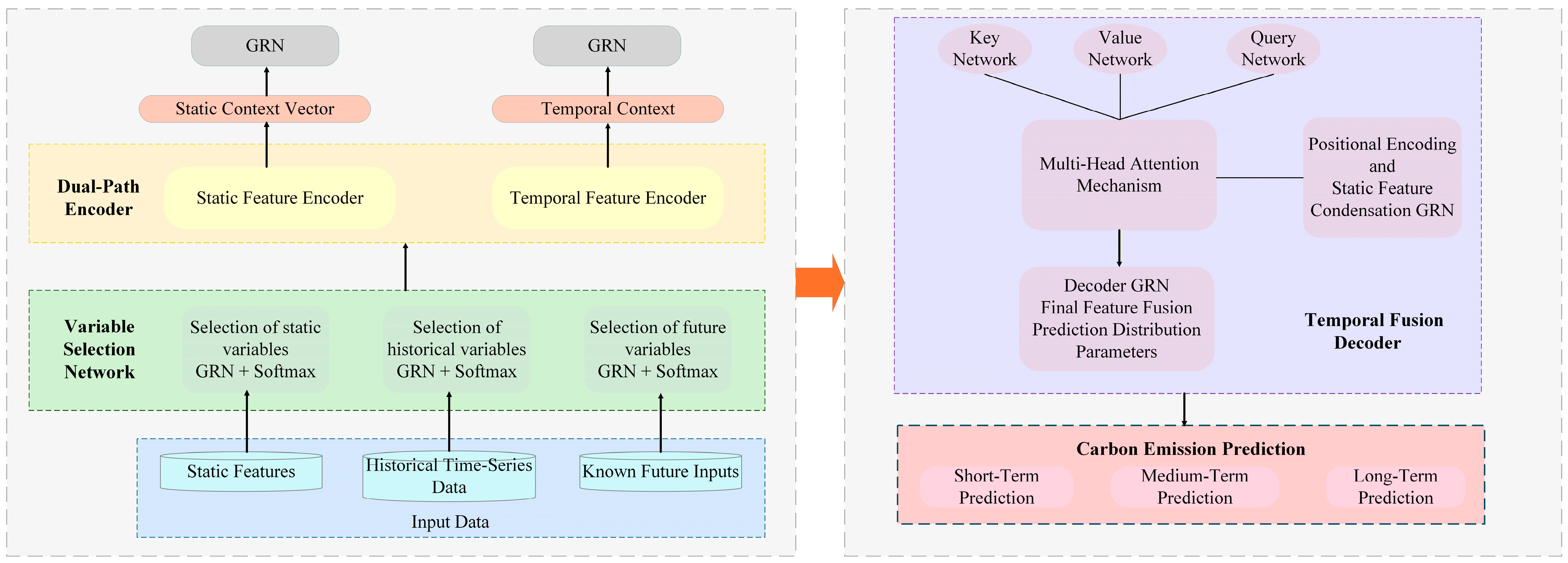
The Temporal Fusion Transformer (Figure 2) is a time series forecasting model based on the Transformer architecture, suitable for multivariate time series prediction tasks. This model integrates an attention mechanism, an encoder–decoder structure, and interpretability components. It effectively captures long-term dependencies within temporal data, complex interactions between static and dynamic variables, and identifies the contribution of key time steps and features to the prediction outcome.

a.

Categorizing Input Variables: The input variables need to be divided into three categories according to the temporal framework of the TFT model: static covariates, past (historical) covariates, and future (known) covariates. Let the input sequence length be ${\mathrm{T}}_{\mathrm{in}}$, and the output forecast length be ${\mathrm{T}}_{\mathrm{out}}$.

①

Static Covariates: $S_i\in R^{D_S}$, where $D_s$ is the dimension of static variables.

②

Past (Historical) Covariates: $X_i=\{X_{i,t-T_{\mathrm{in}}+1},X_{i,t-T_{\mathrm{in}}+2},\dots ,X_{i,t}\}\in R^{T_{\mathrm{i}\mathrm{n}}\times D_X}$;

③

Future (Known) Covariates: $Y_i^{\mathrm{pred}}=\{Y_{i,t+1},\dots ,Y_{i,t+T_{\mathrm{out}}}\}\in R^{T_{\mathrm{out}}}$.

b.

Feature Selection Network: The TFT employs a variable selection mechanism to automatically identify important features, filter out redundant information, and enhance the model’s interpretability.

$${v }_{{\chi }_t}=\mathit{Softmax}\left(\mathit{GRN}\left({\chi }_t,s\right)\right)$$

(9)

In Formula (9), ${\chi }_t$ represents the input features, GRN denotes the gated residual network, and ${v }_{{\chi }_t}$ is a probability distribution vector where each element corresponds to the importance weight of an input feature at the current time step t.

$$\mathit{GRN}\left(a,c\right)=\mathit{LayerNorm}\left(a+\mathit{GLU}\left({\eta }_1\right)\right)$$

(10)

$${\eta }_1=W_1{\eta }_2+b_1$$

(11)

$${\eta }_2=\mathit{ELU}\left(W_{2}a+W_{3}c+b_2\right)$$

(12)

In Formulas (10) to (12), $a$ is the primary input; LayerNorm represents standard layer normalization; ${\eta }_1$ and ${\eta }_2$ denote the outputs of intermediate layer transformations; ELU is the Exponential Linear Unit activation function; $W_1,W_2,W_3$ are learnable weight matrices acquired through training; and $b_1,b_2$ are bias vectors that provide offset capabilities to the network.

$$\mathit{GLU}\left(\gamma \right)=\sigma \left(W_4\gamma +b_4\right)\odot \left(W_5\gamma +b_5\right)$$

(13)

In Formula (13), GLU refers to the Gated Linear Unit, $\gamma$ is the input of GLU; $W_4,W_5$ are the weight matrices of GLU; $b_4,b_5$ are the bias vectors of GLU; $\sigma \left(\cdot \right)$ is the sigmoid function, with an output range of [0, 1], serving as the gating signal; $\odot$ denotes the Hadamard product, which uses the sigmoid output to control the flow of information.

c.

Temporal Attention Mechanism: The Temporal Fusion Transformer (TFT) employs a multi-head self-attention mechanism to learn the long-term relationships between different time steps. This mechanism is used to capture differences in the importance of historical time steps, focus on critical time points, and enhance interpretability.

$$\mathit{Attention}\left(Q,K,V\right)=\mathit{Softmax}\left({\displaystyle \frac{{QK}^T}{\sqrt{d_k}}}\right)V$$

(14)

In Formula (14),$Q$ is the query vector, which can be understood as a question posed by the current time step (or position); $K$ is the key vector, representing a summary of each element in the sequence for matching with the query; $V$ is the value vector, representing the information content of each element in the sequence; ${QK}^T$ is the matching degree calculation, which computes the dot product of the query vector $Q$ and all key vectors $K$ to measure the similarity between the two vectors; ${\displaystyle \frac{{QK}^T}{\sqrt{d_k}}}$ denotes scaling, which is performed to stabilize training and maintain the health of gradients.

$$\mathit{MultiHead}\left(Q,K,V\right)=\left[{\mathit{head}}_1,\dots ,{\mathit{head}}_H\right]W^O$$

(15)

$${\mathit{head}}_i=\mathit{Attention}\left({QW}_i^Q,{KW}_i^K,{VW}_i^V\right)$$

(16)

Formula (15) represents the concatenation of the outputs of all heads to obtain the final multi-head attention output, where $W^O$ is another learnable parameter matrix; $\left[{\mathrm{head}}_1,\dots ,{\mathrm{head}}_H\right]$ denotes the concatenation of the output vectors of H attention heads. Formula (16) describes how to generate the i attention head, where $W_i^Q,W_i^K,W_i^V$ are learnable parameter matrices trained specifically for the i head.

d.

Fusion Decoder: It integrates static features, historical information, and future information.

$$\widetilde{h_t}=\mathit{LayerNorm}\left(h_t+\mathit{MultiHead}\left(h_t,h_{\le t},h_{\le t}\right)\right)$$

(17)

In Formula (17), $h_t$ represents the current hidden state of the decoder at time step t; ${\mathrm{h}}_{\le \mathrm{t}}$ represents the sequence of hidden states from all historical time steps (up to time t) output by the encoder.

e.

Loss Function: This enables the model not only to predict the most probable value but also to quantify the uncertainty of the prediction, which is crucial for decision-making problems in carbon emission prediction.

$$\mathcal{L}=\sum _{t=1}^T\sum _{q\in \mathcal{Q}}{\displaystyle \frac{2\cdot \mathit{QL}\left(y_t,\widehat{y_t}\left(q\right),q\right)}{{\sum }_{t=1}^T\left|y_t\right|}}$$

(18)

$$\mathit{QL}\left(y,\widehat{y},q\right)=\mathit{max}\left(q\left(y-\widehat{y}\right),\left(1-q\right)\left(\widehat{y}-y\right)\right)$$

(19)

Formula (18) is the overall standardized loss function, where T is the total number of time steps; Q is the set of target quantiles; ${\sum }_{t=1}^T\left|y_t\right|$ is the normalization factor.

Formula (19) is the quantile loss function, which is the core calculation unit of the entire loss function. $y$ denotes the true value, $\widehat{y}\left(q\right)$ is the predicted value; $q$ is the target quantile; QL is the quantile loss. When the true value is greater than the predicted value, the loss is $q\left(y-\widehat{y}\right)$; when the true value is less than the predicted value, the loss is $\left(1-q\right)\left(\widehat{y}-y\right)$.

In this paper, the input of the TFT model fully reflects the multidimensional characteristics of the EEC framework. Static covariates are defined as provincial individual characteristics; historical covariates are set as the time series of energy variables (E1–E3) and economic variables (J1–J2); future-known covariates are specified as time encodings; and total carbon emissions (C1) serve as the target sequence for model prediction.

3.2.2. ASTGCN

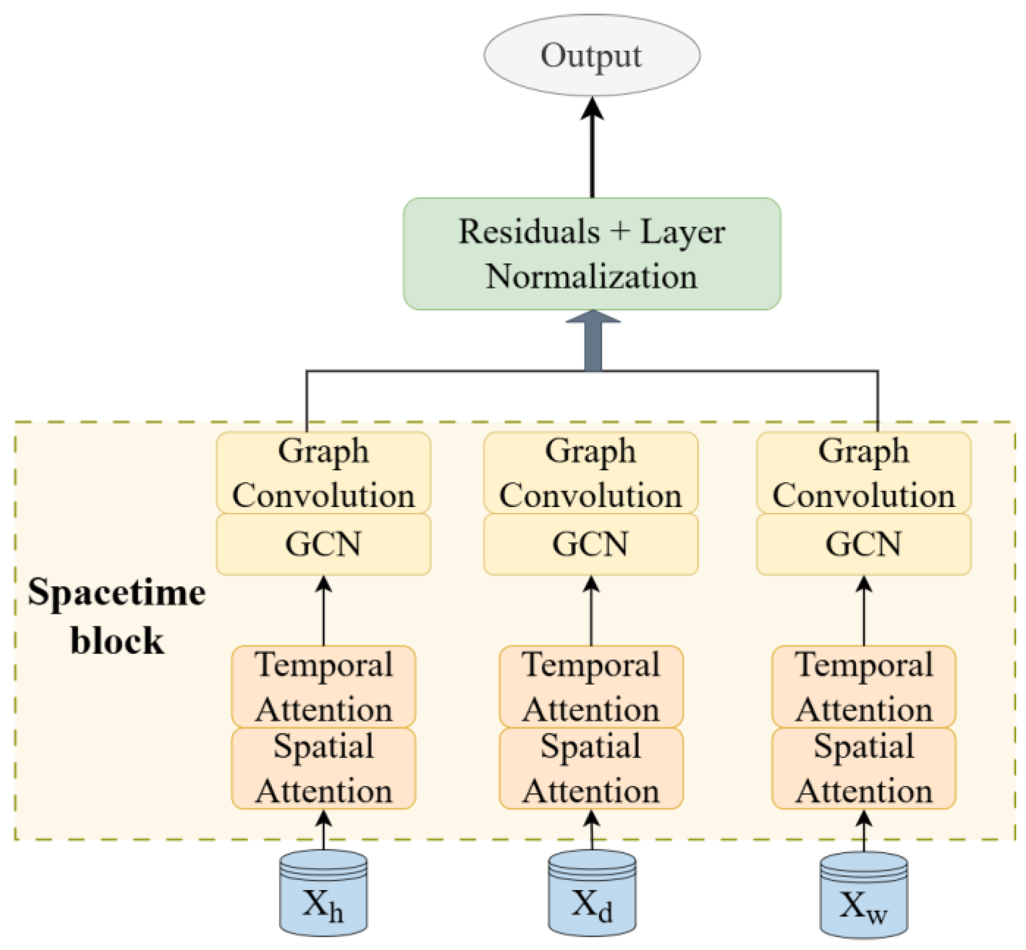
In this study, while the TFT model excels in temporal modeling, it struggles to adapt to the spatial correlation characteristics of regional carbon emissions. In contrast, ASTGCN compensates for the TFT model’s limitations in the spatial dimension through its graph structure and spatiotemporal co-design. The combination of both enables comprehensive prediction across both temporal and spatial dimensions. ASTGCN (Figure 3) is a deep learning model specifically designed for spatiotemporal sequence data. Its core strength lies in capturing spatial correlations through graph convolutional layers, temporal dependencies through temporal convolutional layers, and enhancing the weights of key spatiotemporal features via an attention mechanism. This makes it well-suited for the task of predicting regional carbon emissions across the nine provinces of the Yellow River Basin, which involve geographical linkages and dynamic developmental disparities. The model can effectively integrate the spatial proximity of provincial administrative units, energy-economic linkages, and the temporal evolution patterns of carbon emissions, addressing the challenges of spatial heterogeneity and temporal dynamics that are difficult for traditional models to handle simultaneously.

a.

Define Spatiotemporal Graph Structure: Define an undirected graph G.

$$G=\left(V,E,A\right)$$

(20)

In Formula (20), $V$ denotes the set of nodes in the graph; $E$ is the set of edges in the graph, representing spatial associations between provinces; $A$ is the adjacency matrix, with $A\in R^{N\times N}$.

b.

Normalization: To avoid convolution bias caused by differences in node degrees, normalization is required.

$$\tilde{A}=A+I$$

(21)

$$\widetilde{D_{ii}}=\sum _j\widetilde{A_{ij}}$$

(22)

$$\mathcal{L}={\tilde{D}}^{-{\displaystyle \frac{1}{2}}}\tilde{A}{\tilde{D}}^{-{\displaystyle \frac{1}{2}}}\in R^{N\times N}$$

(23)

Formulas (21) to (23) obtain the Laplacian matrix $\mathcal{L}$ by adding self-loops to the adjacency matrix and performing symmetric normalization. Subsequent graph convolution operations are based on this matrix, ensuring that node features maintain stable spatial structure and numerical values during propagation.

c.

Spatial Attention: Calculate the real-time influence weight matrix S between provinces using current data, then multiply it element-wise with the static adjacency matrix to obtain a dynamic adjacency matrix, enabling graph convolution to adaptively adjust spatial associations according to input.

$$S^{\left(l\right)}=\mathit{Softmax}\left(X_t{W}_s^{\left(l\right)}{X}_t^{\top }\right)\in R^{N\times N}$$

(24)

$$\widetilde{{\mathcal{L}}^{\left(l\right)}}=\mathcal{L}\odot S^{\left(l\right)}$$

(25)

In Formula (24), for any time slice $X_t\in R^{N\times D}$, $W_s^{\left(l\right)}$ is a learnable weight matrix with $W_s^{\left(l\right)}\in R^{D\times D}$; $S^{\left(l\right)}$ is the attention weight matrix, where $S^{\left(l\right)}$ represents the influence weight of province j on province i.

Formula (25) indicates that the static graph structure $\mathcal{L}$ is multiplied element-wise with the dynamic attention weight $S^{\left(l\right)}$ to obtain the dynamic adjacency matrix $\widetilde{{\mathcal{L}}^{\left(l\right)}}$.

d.

Graph Convolution: Perform a graph convolution on the features of each province using the dynamic adjacency matrix $\widetilde{{\mathcal{L}}^{\left(l\right)}}$ of the current layer to output new spatial representations $H_{\mathrm{space}}^{\left(l\right)}$, completing the propagation of dynamic graph convolution features.

$$H_{\mathit{space}}^{\left(l\right)}=\sigma \left(\widetilde{{\mathcal{L}}^{\left(l\right)}}{H}^{\left(l\right)}{W}_{\mathit{gcn}}^{\left(l\right)}\right)$$

(26)

In Formula (26), $H^{\left(l\right)}$ denotes the node features input to the $l$ layer; $W_{\mathrm{gcn}}^{\left(l\right)}$ is the learnable weight matrix for the $l$ layer of graph convolution, responsible for linear transformation.

e.

Temporal Attention: The Softmax function is used to convert the similarity between historical time points into normalized weights, yielding a dynamic temporal correlation matrix for subsequent convolution to fuse historical information according to importance.

$$T^{\left(l\right)}=\mathit{Softmax}\left(X^{\prime }{W}_t^{\left(l\right)}{X}^{\prime \top }\right)\in R^{T\times T}$$

(27)

In Formula (27), $X^{\prime }\in R^{T\times d^{\prime }}$ represents the feature sequence of a specific province over the entire time window; $W_t^{\left(l\right)}$ is the learnable temporal attention weight matrix for the $l$ layer; $T^{\left(l\right)}$ denotes the output temporal attention matrix.

f.

Temporal Convolution: Historical sequences are weighted and filtered using temporal attention weights, and long-term temporal dependencies are extracted via causal dilated convolution to obtain new temporal features containing key period information.

$$H_{\mathit{time}}^{\left(l\right)}=\mathit{ReLU}\left(\mathit{Conv}1\mathit{D}\left(T^{\left(l\right)}\odot X^{\prime }\right)\right)$$

(28)

In Formula (28), $X^{\prime }$ is the temporal feature of the current province; Conv1D refers to 1D causal dilated convolution; ReLU is the activation function that introduces non-linearity. This formula employs causal dilated convolution, where the dilation factor grows exponentially with the layer depth.

g.

Residual Connection: Deep temporal features are fused with the original representation via residual connections, and distribution correction is performed through layer normalization to ensure smooth gradient backpropagation and improve training stability.

$$H^{\left(l+1\right)}=\mathit{LayerNorm}\left(H^{\left(l\right)}+H_{\mathit{time}}^{\left(l\right)}\right)$$

(29)

h.

Loss Function: The quantile loss is adopted, which is consistent with the loss function of the TFT model (Formula (18)).

i.

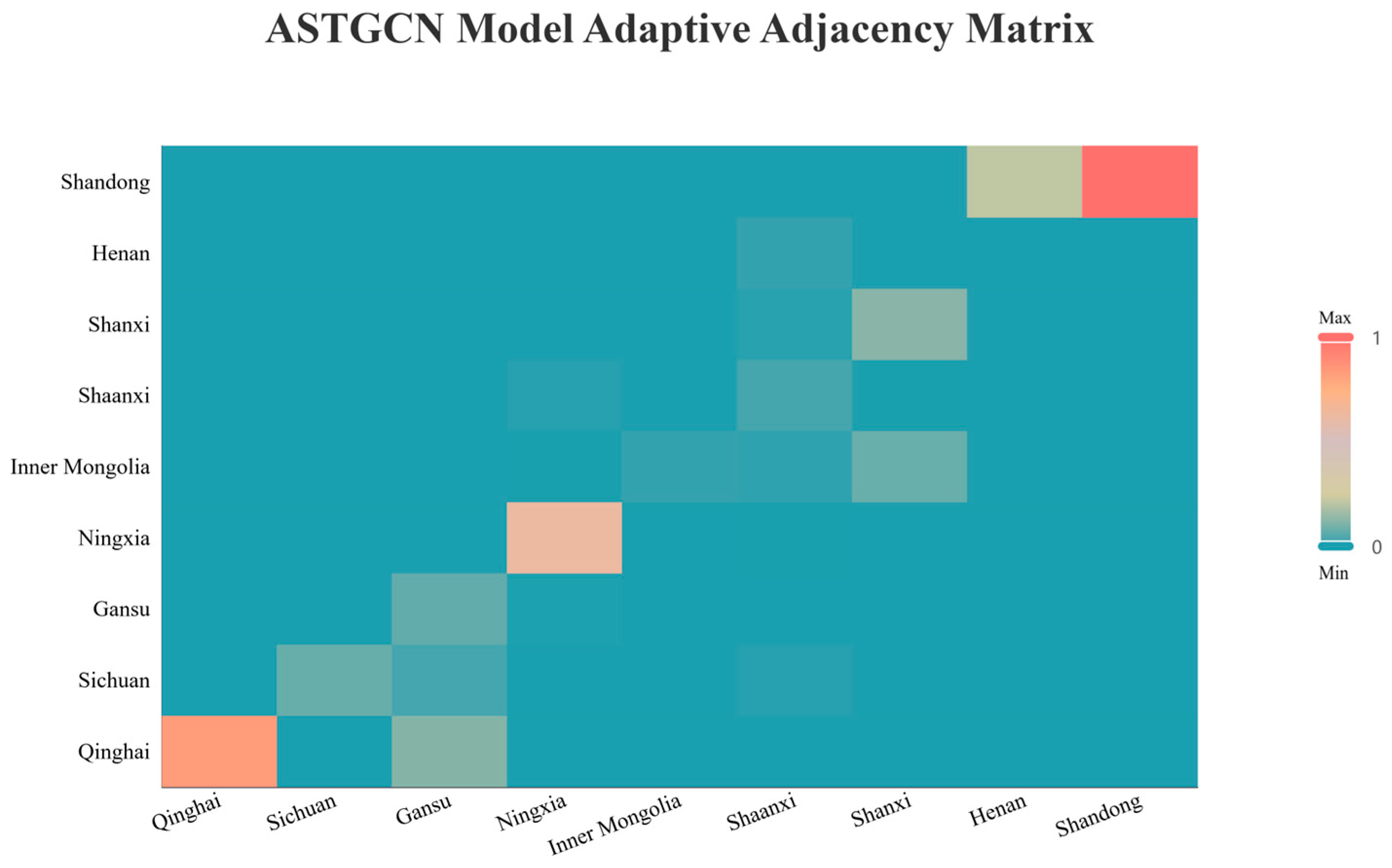
Adaptive Adjacency Matrix: To dynamically capture the real-time spatial correlations of carbon emissions among provinces, the model incorporates an adaptive adjacency matrix mechanism. This mechanism first calculates dynamic attention weights between provinces based on the current input features through learnable parameter matrices (Equation (24)). This weight matrix possesses asymmetry, enabling it to capture the unidirectional propagation of spatial influences. Subsequently, these dynamic weights are element-wise multiplied with a prior static adjacency matrix $\widetilde{{\mathcal{L}}^{\left(l\right)}}$ that integrates geographical, energy, and economic linkages to generate the final dynamic adjacency matrix for spatial information propagation (Equation (25)). This matrix overcomes the limitations of traditional fixed spatial weights, allowing the model to adaptively adjust the strength and direction of inter-provincial associations based on the data. Consequently, it more accurately characterizes the dynamism and heterogeneity of the spatial spillover effects in carbon emissions.

3.3. Data Sources

This study selects the nine provinces of the Yellow River Basin as the research area, with a time span from 2005 to 2022. The energy and economic data were sourced from provincial statistical yearbooks, while the carbon emission data were obtained from the province-level datasets of the China Emission Accounts and Datasets (CEADs) [40,41,42,43,44].

4. Analysis

4.1. Analysis of Spatial Durbin Model Results

4.1.1. Moran’s I Test

To investigate whether carbon emissions exhibit spatial autocorrelation, both global and local Moran’s I tests were conducted based on the defined spatial weights. The results of the global Moran’s I test, as shown in

Table 3. Global Moran’s I Test.

Year	Morani	p	Z	Year	Morani	p	Z
2005	0.5533	0.0002	3.7696	2014	0.2354	0.0027	3.0558
2006	0.5395	0.0001	3.7296	2015	0.4251	0.0059	3.0013
2007	0.5318	0.0001	3.7571	2016	0.4694	0.0065	3.1686
2008	0.5598	0.0001	3.7983	2017	0.4612	0.0066	3.0067
2009	0.5350	0.0004	3.6970	2018	0.4467	0.0088	2.9966
2010	0.4977	0.0003	3.6516	2019	0.4128	0.0124	2.7906
2011	0.4873	0.0009	3.5105	2020	0.4207	0.0095	2.8986
2012	0.2362	0.0020	3.0767	2021	0.4975	0.0064	3.2245
2013	0.4909	0.0027	3.3789	2022	0.3569	0.0224	2.1714

, indicate a positive spatial correlation of carbon emissions, demonstrating significant spatial dependence among neighboring provinces.

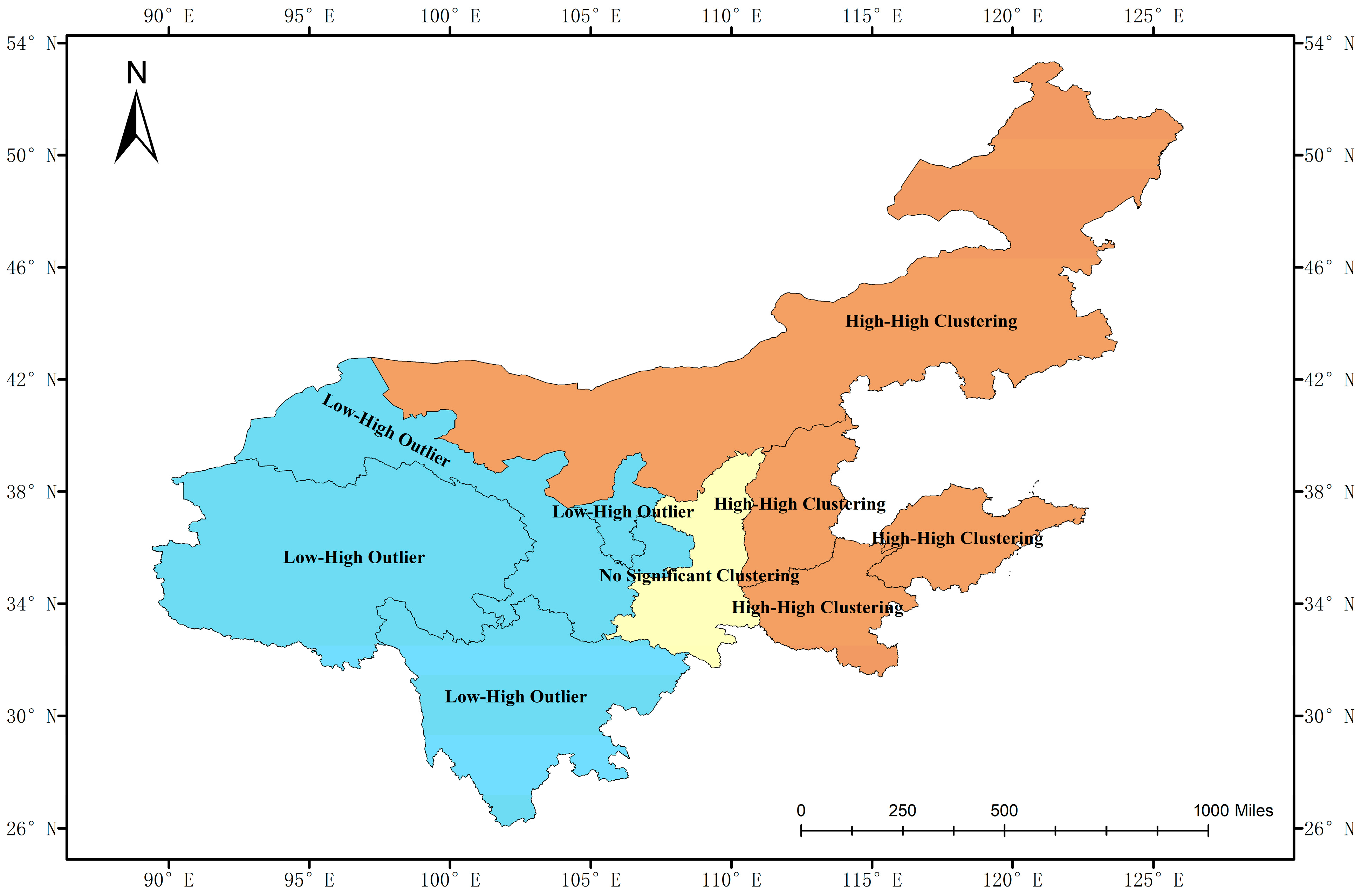
The results of the Local Moran’s I test are shown in Figure 4. The test indicates the clustering type for each province, revealing a spatial clustering pattern in carbon emissions among the provinces.

4.1.2. Results of the Spatial Durbin Model

The Moran’s I test indicates the presence of spatial correlation among energy, economy, and carbon emissions. Therefore, based on the results of the LM, LR, and Hausman tests (

Table 4. Spatial Panel Model Tests.

Test Name	Statistic	p-Value	Result
LM Error Test	257.8392	0.0000	Significant
LM Lag Test	8.6259	0.0033	Significant
Hausman Test	1145.7186	0.0000	Significant
Likelihood Ratio Test	9.0602	0.0026	Significant
Wald Test	8.5131	0.0035	Significant

), this study selects the Spatial Durbin Model. After testing for time-fixed effects, individual fixed effects, and two-way fixed effects, the time-fixed effect Spatial Durbin Model is ultimately chosen for this analysis.

SDM includes spatial lag terms, the estimated coefficients cannot directly and precisely reflect the impact of independent variables on the dependent variable. Therefore, drawing on relevant literature [45,46], this study decomposes the total effect into direct and indirect effects. The results are shown in

Table 5. Decomposition of Spatial Effects from the SDM.

Original Indicator	Direct Effect	Indirect Effect	Total Effect
Lagged Term of Carbon Emissions	0.3642 *** (0.0966)	0.0063 (0.0159)	0.3701 *** (0.0983)
Regional Gross Domestic Product	0.0142 (0.0762)	−0.0213 (0.0158)	−0.0071 (0.0715)
Proportion of Added Value in the Secondary Industry	0.1105 (0.1400)	0.0707 ** (0.0338)	0.1812 (0.1644)
Total Energy Consumption	0.5050 *** (0.0922)	0.0036 (0.0194)	0.5086 *** (0.0895)
Proportion of Fossil Fuel Production	−0.0346 (0.1364)	−0.0576 (0.0404)	−0.0922 (0.1286)
Proportion of Coal Consumption	0.3072 *** (0.0925)	0.0062 (0.0265)	0.3146 *** (0.1058)

Note: ** and *** denote statistical significance at the 5% and 1% levels, respectively.

(standard errors are in parentheses).

According to the SDM results, carbon emissions exhibit significant path dependence. The direct effect coefficient of the one-period lagged carbon emissions is 0.3642 and is statistically significant at the 1% level, indicating a significant positive direct impact of past emissions on current emissions. This suggests a strong carbon lock-in effect within the carbon emission systems of the provinces, where historical emission patterns persistently influence current emission behaviors. Energy consumption is the most critical driver of carbon emissions. The direct effect of total energy consumption on local carbon emissions is 0.5050, significant at the 1% level, indicating that the scale of energy demand is a major force driving carbon emission growth. The proportion of coal consumption also shows a significant positive direct effect, further confirming that the high-carbon nature of the energy structure is a key factor exacerbating emissions. However, the indirect effects of these two variables are not significant, suggesting their influence is primarily confined within provincial boundaries and does not generate significant cross-provincial spatial spillovers. The impact of the proportion of fossil energy production on carbon emissions is not significant. This may be related to regional differences in energy transfers and consumption structures within the Yellow River Basin, where structural indicators from the production side do not directly translate into emission pressure on the consumption side.

The influence of economic factors on carbon emissions presents a certain degree of spatial complexity. Although the proportion of value-added from the secondary industry shows no significant direct effect, its indirect effect is 0.0707 and significant at the 5% level. This indicates that increased industrial development in neighboring provinces exerts a positive spatial spillover effect on a province’s own carbon emissions. In contrast, Gross Regional Product shows no statistical significance in direct, indirect, or total effects, suggesting that economic growth itself has a weak marginal impact on carbon emissions.

4.2. Analysis of System GMM

4.2.1. System GMM Results

While the SDM effectively captures the spatial correlation characteristics and spillover effects of carbon emissions among the nine provinces in the Yellow River Basin, it has limitations in addressing potential bidirectional causality (endogeneity) and dynamic path dependence within the EEC system. These limitations make it difficult to precisely isolate the true causal relationships among variables. To overcome the shortcomings of the SDM and enhance the robustness and reliability of the conclusions, this study introduces the system GMM model for in-depth analysis of the dynamic panel data. By selecting appropriate instrumental variables to mitigate endogeneity concerns and incorporating a lagged term for carbon emissions to reflect its path-dependent nature, the model more accurately identifies the true impact coefficients of energy consumption and economic development on carbon emissions. This provides stronger empirical support for analyzing the dynamic linkage mechanisms among these three dimensions.

Since autocorrelation and Hausman tests were already conducted for the Spatial Durbin Model, this section directly presents the test results for the System GMM. The specific results are shown in

Table 6. Test Results of the Impact of Energy and Economy on Carbon Emissions.

Original Indicator	OLS	2SLS	System GMM
Constant Term	0.0547 *** (0.0085)	0.0542 *** (0.0085)	0.0548 *** (0.008)
Lagged Term of Carbon Emissions	0.9207 *** (0.0366)	0.8924 *** (0.0399)	0.8990 *** (0.0361)
Regional Gross Domestic Product	−0.0772 *** (0.0220)	−0.0856 *** (0.0225)	−0.0842 *** (0.0218)
Proportion of Added Value in the Secondary Industry	−0.0167 (0.0125)	−0.0204 (0.0127)	−0.0204 (0.0126)
Total Energy Consumption	0.1450 *** (0.0228)	0.1777 *** (0.0503)	0.1707 *** (0.0434)
Proportion of Fossil Fuel Production	0.0264 (0.0228)	0.0296 (0.0229)	0.0300 ** (0.0150)
Proportion of Coal Consumption	0.0086 (0.0219)	0.0109 (0.0220)	0.0098 * (0.0149)

Note: *, **, and *** denote statistical significance at the 10%, 5%, and 1% levels, respectively.

.

The results show that carbon emissions exhibit a strong path-dependent characteristic, with the coefficient for their one-period lag in the system GMM reaching as high as 0.8990, which is highly significant at the 1% level. This indicates a pronounced carbon lock-in effect within the carbon emission system of the Yellow River Basin, implying that emission reduction policies must focus on breaking this structural inertia to drive long-term and fundamental transformation. Energy variables are the most robust drivers of carbon emissions. The coefficient for total energy consumption in the system GMM is 0.1707, significant at the 1% level. Its estimated value is higher than that from the OLS results, suggesting that after controlling for endogeneity, the promoting effect of energy consumption may have been underestimated by traditional methods. Additionally, the proportion of fossil energy production and the proportion of coal consumption achieve significance at the 5% and 10% levels, respectively, in the System GMM, whereas they were not significant in the OLS. This demonstrates that, after accounting for endogenous interactions, both the supply and demand sides of energy exert independent and significant positive impacts on carbon emissions. The coefficient for gross regional product in the system GMM is −0.0842, which is significantly negative at the 1% level. Complementing the findings from the SDM, the system GMM provides new insights regarding economic variables. The results reveal that, after controlling for factors such as energy consumption, gross regional product shows a significant negative correlation with carbon emissions. This finding suggests that for the Yellow River Basin, economic growth itself may have begun to exhibit preliminary signs of decoupling from carbon emission intensity. However, the impact of the proportion of value-added from the secondary industry, while negative, is not statistically significant. This indicates that its high-carbon attribute may more indirectly influence emissions by driving energy consumption as a mediating channel, with its direct marginal contribution being less pronounced at the current stage.

By comparing the results of the SDM and the system GMM model, it can be observed that the two types of models exhibit both commonalities and differences in revealing the impact mechanisms of carbon emissions in the nine provinces of the Yellow River Basin. The commonality lies in the fact that both models confirm that total energy consumption and the proportion of coal consumption have a significant positive promoting effect on carbon emissions. This indicates that, whether from the perspective of spatial correlation or dynamic endogeneity, energy scale and energy structure are key and robust factors influencing regional carbon emissions.

The differences are primarily manifested in the following aspects: Firstly, regarding carbon emission dynamics, the system GMM model reveals an extremely strong path dependence, with a coefficient for the one-period lag of carbon emissions as high as 0.8990, significant at the 1% level. In contrast, in the SDM, the direct effect of the lagged carbon emission term is 0.3642. Although also significant, its magnitude is considerably lower than the system GMM estimates. Furthermore, the system GMM finds that, after controlling for endogeneity, system GMM reveals that the proportion of fossil energy production and coal consumption become statistically significant. This suggests that the influence of structural factors on the energy supply side becomes more prominent when bidirectional causality is considered. Secondly, in the spatial dimension, the unique strength of the SDM lies in its ability to decompose the direct and indirect effects of variables. The results show that the proportion of value-added from the secondary industry exhibits a significant positive spatial spillover effect, revealing the synergistic pressure on carbon emissions arising from industrial linkages across regions. Conversely, the system GMM model, as it does not incorporate a spatial weight matrix, cannot capture such cross-regional spatial interactive influences. Therefore, its analysis focuses more on the dynamic causal mechanisms within individual units. Thirdly, concerning the impact of economic growth, the two models provide complementary perspectives. In the SDM, the direct, indirect, and total effects of gross regional product are all insignificant. However, the system GMM model, after controlling for endogeneity, identifies a significant negative correlation between gross regional product and carbon emissions (coefficient of −0.0842). This indicates that, after isolating mediating factors like energy consumption and mitigating reverse causality, economic growth itself may exhibit a preliminary trend of from carbon emission intensity.

In summary, the SDM and the system GMM model provide complementary evidence from the dimensions of spatial correlation and dynamic endogeneity, respectively. The SDM emphasizes the importance of cross-regional spillovers of variables, while the system GMM model more precisely characterizes the dynamic adjustment process of carbon emissions itself and the causal relationships among variables. Integrating the two models offers more comprehensive and robust empirical support for understanding the complex mechanisms of the EEC system.

4.2.2. Robustness Test

To further validate the effectiveness of the system GMM results, this study conducted a robustness test for the system GMM (the results are shown in

Table 7. Results of System GMM Robustness Tests.

Original Indicator	Substitution of the Core Variable	Adjustment of the Sample Interval
Constant Term	0.0548 *** (0.0080)	0.0548 *** (0.0080)
Lagged Term of Carbon Emissions	——	0.8800 *** (0.0370)
Regional Gross Domestic Product	−0.1200 *** (0.0250)	−0.0900 *** (0.0230)
Proportion of Added Value in the Secondary Industry	−0.0150 (0.0130)	−0.0180 (0.0128)
Total Energy Consumption	0.1800 *** (0.0450)	0.1650 *** (0.0440)
Proportion of Fossil Fuel Production	0.0250 (0.0160)	0.0280 (0.0155)
Proportion of Coal Consumption	0.0080 (0.0150)	0.0105 (0.0152)
AR(1) test p-value	0.0042	0.0050
AR(2) test p-value	0.3500	0.2800
Sargan	0.8500	0.7500

Note: *** denote statistical significance at the 1% levels.

). The reliability of the model was verified in two ways: first, by replacing the core variable (substituting the dependent variable from total carbon emissions to carbon emission intensity, C1/J1); second, by adjusting the sample period (shortening the study timeframe to 2008–2022). The results show that the key conclusions of the model remain stable under both tests, indicating that the baseline regression results possess good robustness.

In the robustness check involving the substitution of the core variable, where the dependent variable is replaced by carbon emission intensity, the lagged term of carbon emissions is excluded from the model, while the coefficient signs of other variables remain consistent with those in the baseline model: the coefficient of regional GDP is −0.1200, still showing a significantly negative effect, and the coefficient of total energy consumption is 0.1800, maintaining a significantly positive influence. This indicates that even when using carbon emission intensity as a relative indicator, energy consumption remains a core driver of carbon emissions, while economic growth exhibits a certain decoupling trend.

In the test with an adjusted sample period, after shortening the study timeframe, the coefficient of the lagged carbon emission term is 0.8800, still indicating strong path dependence; the coefficient of regional GDP is −0.0900, and that of total energy consumption is 0.1650, with no fundamental changes in their signs or significance. This suggests that the research conclusions are adaptable to different time windows and are not substantially biased due to the selection of the sample period.

Diagnostic statistics from both tests meet the validity requirements of the system GMM estimation: the p-value of the AR(1) test is below 0.05, indicating first-order autocorrelation in the residuals; the p-value of the AR(2) test exceeds 0.05, suggesting the absence of second-order autocorrelation; and the p-value of the Sargan test is greater than 0.05, confirming instrument validity and no over-identification issues. These results collectively support the rationality of the model specification and the reliability of the estimation outcomes.

The robustness tests in Table 7 provide additional evidence for the main findings of this study: carbon emissions in the Yellow River Basin exhibit significant path dependence, with energy consumption being a key driving factor, while economic growth and carbon emissions show initial signs of decoupling.

4.3. Temporal Fusion Transformers Results Analysis

4.3.1. Dataset Experiments

In the empirical analysis using the SDM and system GMM in the previous section, energy consumption and structural indicators were confirmed as core factors driving carbon emissions in the nine provinces of the Yellow River Basin, with both their direct impacts and spatial spillover effects being significant. In contrast, while economic indicators did not show an overall significant influence in the SDM, the proportion of value-added from the secondary industry exhibited significance in the indirect effects, and regional GDP demonstrated excellent significance in the system GMM model. This indicates a potential association between economic activity and carbon emissions. To more comprehensively capture potential nonlinearities, interactions, and dynamic temporal characteristics within this system, this study further introduces the TFT model. The TFT possesses powerful capabilities for multivariate time series modeling and feature selection mechanisms. While retaining economic variables, it can automatically identify their conditional contributions and intertemporal impacts on carbon emissions. Consequently, within a machine learning framework, it provides more nuanced and interpretable temporal insights into the co-evolution of the EEC system.

To evaluate the predictive performance of the TFT model employed in this study, representative baseline models are selected for comparison. LSTM, a classic variant of recurrent neural networks, is widely used to capture temporal dependencies; Transformer, as the foundational architecture of TFT, is employed to validate the effectiveness of incorporating gating mechanisms and variable selection modules; and the traditional time series model ARIMA is used to assess the relative advantages of deep learning approaches. The appropriateness of the TFT model is evaluated by comparing the Mean Absolute Error (MAE), Root Mean Square Error (RMSE), and the Coefficient of Determination (R²). The comparative results of model performance are presented in

Table 8. Comparison of Results from Different Models.

Model Type	MAE	RMSE	R2
TFT	0.2146	0.2906	0.8793
LSTM	0.2653	0.3351	0.8201
ARIMA	0.3217	0.3999	0.7648
Transformer	0.3157	0.4107	0.7833

.

The experimental results in Table 8 indicate that the TFT model performs best on both the RMSE and R² metrics. Its RMSE is 0.2906, lower than all other models, and its R² reaches 0.8793, demonstrating that the TFT model possesses the strongest fitting capability and predictive stability. Although ARIMA slightly outperforms Transformer in terms of RMSE, its overall predictive performance is significantly inferior to TFT, reflecting the limitations of traditional time series models in characterizing multi-factor, nonlinear interactive systems such as the Energy-Economy-Carbon Emissions nexus. While LSTM and Transformer are deep learning models, their ability to capture long-term dependencies and multivariate co-evolution remains weaker than TFT’s without incorporating feature selection and structured attention mechanisms.

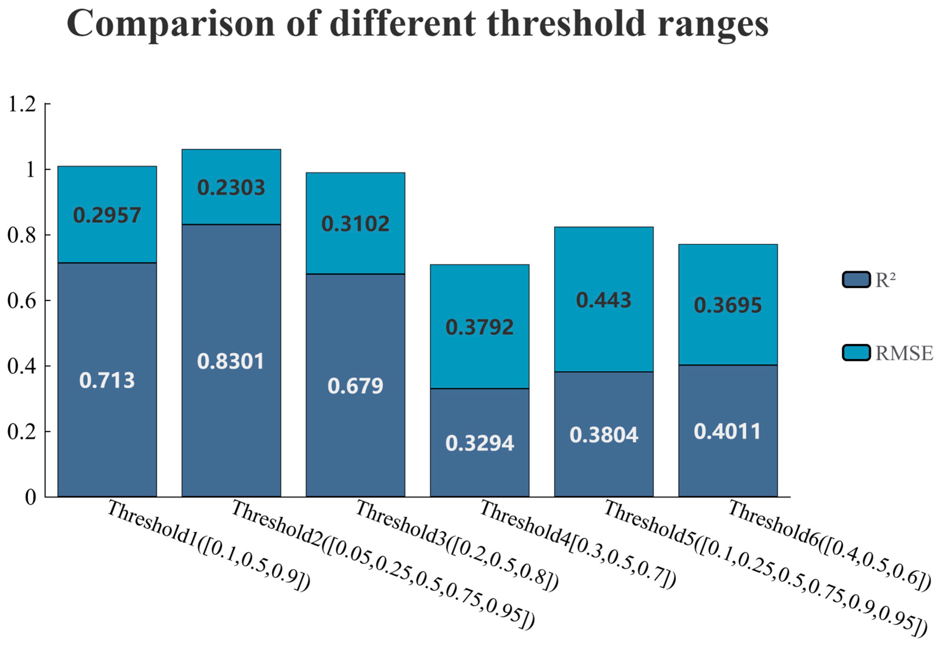
To further validate the stability and generalization capability of the TFT model under different data partitioning strategies, this study designs six distinct quantile combination strategies (as shown in Figure 5). These quantile combinations, ranging from sparse to dense and from wide to narrow intervals, systematically evaluate the model’s predictive performance across various confidence levels. The results indicate that Threshold Set 2 delivers superior performance, achieving an R² of 0.8301, which is higher than all other sets, and the lowest RMSE of 0.2303. This demonstrates that the finer quantile grid employed in this study can more comprehensively capture both the tail characteristics and the central tendency of the data distribution, thereby enhancing the model’s capability to fit complex dynamic systems. In contrast, the traditional tercile-based Threshold Set 1, while robust, lacks the granularity required for finely characterizing tail events. Conversely, narrow interval settings that are excessively concentrated on the central region, such as Threshold Sets 4 and 6, lead to a significant decline in predictive performance due to a severe underestimation of actual volatility. The findings further reveal that merely increasing the number of quantiles does not consistently improve performance. For instance, Threshold Set 5 achieves an R² of 0.3804, which is lower than that of Set 2, indicating a potential risk of over-parameterization.

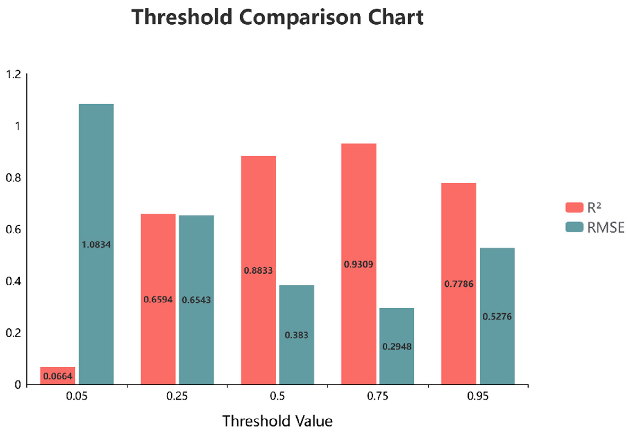
To provide a more detailed examination of the TFT model’s predictive capability across different thresholds, this study further subdivides Threshold Set 2 to evaluate the performance at each individual quantile threshold (as shown in Figure 6). The predictive performance of the TFT model exhibits systematic variation across quantiles, characterized by an olive-shaped pattern where prediction accuracy initially rises rapidly and then declines slowly as the quantile increases.

The results show that under the deep decarbonization scenario corresponding to the extremely low quantile (0.05 quantile), the model’s predictive performance is significantly weaker. This reveals the fundamental uncertainty inherent in trajectories that deviate radically from the current high-carbon pathway. Such paths are primarily constrained by the pace of future breakthrough clean technologies and by nonlinear, forceful climate policy interventions like Carbon Border Adjustment Mechanisms, factors which lie beyond the capture of models relying on extrapolation from historical trends. The region with the strongest and most consistently improving predictive performance as the quantile increases is concentrated in the medium-to-high interval (0.25–0.75 quantiles). The model demonstrates excellent predictive performance at medium-to-high emission levels, with the 0.75 quantile achieving the optimal results—an R² of 0.9309 and an RMSE of 0.2948. This strongly corroborates the findings from the spatial econometric model in this paper: the evolution of carbon emissions, driven primarily by energy consumption, exhibits significant path dependence and systemic inertia. This confirms the existence of a powerful carbon lock-in effect within the current carbon emission system. This lock-in is fundamentally shaped by a series of long-term, consistent industrial and energy policies. Consequently, under business-as-usual or steadily strengthening policy baseline scenarios, carbon emission trajectories possess high predictability, allowing the model to accurately capture their main trends. Under the extremely high quantile scenario (0.95 quantile), while the model’s performance remains relatively strong, it shows a decline compared to the 0.75 quantile. This indicates that if future economic growth were again to become highly reliant on the expansion of traditional energy-intensive industries, the carbon emission path would largely replicate historical inertia and remain partially predictable. However, the higher uncertainty associated with this scenario suggests it might be more susceptible to exogenous shocks or policy reversals, such as severe volatility in global energy markets or the relaxation of environmental regulations to safeguard economic growth.

4.3.2. Ablation Experiments

Ablation experiments were designed to systematically evaluate the specific contribution of each core component within the TFT model to the performance of carbon emission prediction. The experiments were conducted by sequentially removing three key components: the feature selection network, the attention mechanism, and the static context encoder, and then comparing their predictive performance on the test set against that of the full model. The results are presented in

Table 9. Results of Ablation Experiments.

Model	MAE	RMSE	MAPE/%
Complete Model	0.1389	0.1740	27.30
Ablated Feature Selection Network	0.3836	0.4886	60.92
Ablated Attention Mechanism	0.3203	0.4056	55.55
Ablated Static Context	0.6931	0.8644	113.92

. From the perspective of overall performance change, the full model significantly outperformed all ablation variants across the three evaluation metrics—MAE, RMSE, and MAPE. This indicates that the integrated architecture of the TFT model exhibits high synergy and indivisibility when capturing the dynamics of the complex EEC system.

The removal of the feature selection network resulted in the most significant performance decline, with MAE and RMSE increasing to 0.3836 and 0.4886, respectively, and MAPE reaching as high as 60.92%. This demonstrates the indispensable role of the variable selection mechanism in filtering out redundant features and focusing on key driving factors.

The performance loss caused by the absence of the attention mechanism (MAE 0.3203, MAPE 55.55%) underscores the critical importance of evaluating the effectiveness of temporal policy interventions. The attention mechanism enables the model to dynamically focus on key turning periods within historical emission trajectories, such as the implementation phases of stringent environmental regulations like the Air Pollution Prevention and Control Action Plan. The observed performance degradation indicates that without understanding the time-lag effects and cumulative impacts of policy shocks, accurately predicting future emission pathways remains challenging.

The ablation of the static context encoder led to substantial performance deterioration (MAE 0.6931, RMSE 0.8644), profoundly reflecting the spatial heterogeneity challenges that must be addressed in China’s regional collaborative emission reduction efforts. This component encodes the inherent structural characteristics of each province, such as Shandong’s identity as a heavy chemical industry base or Qinghai’s context of abundant clean energy resources. Its significance illustrates that coarse-grained emission reduction policies are largely ineffective in practice, and it is essential to formulate tailored energy-saving and emission-reduction policies adapted to local conditions.

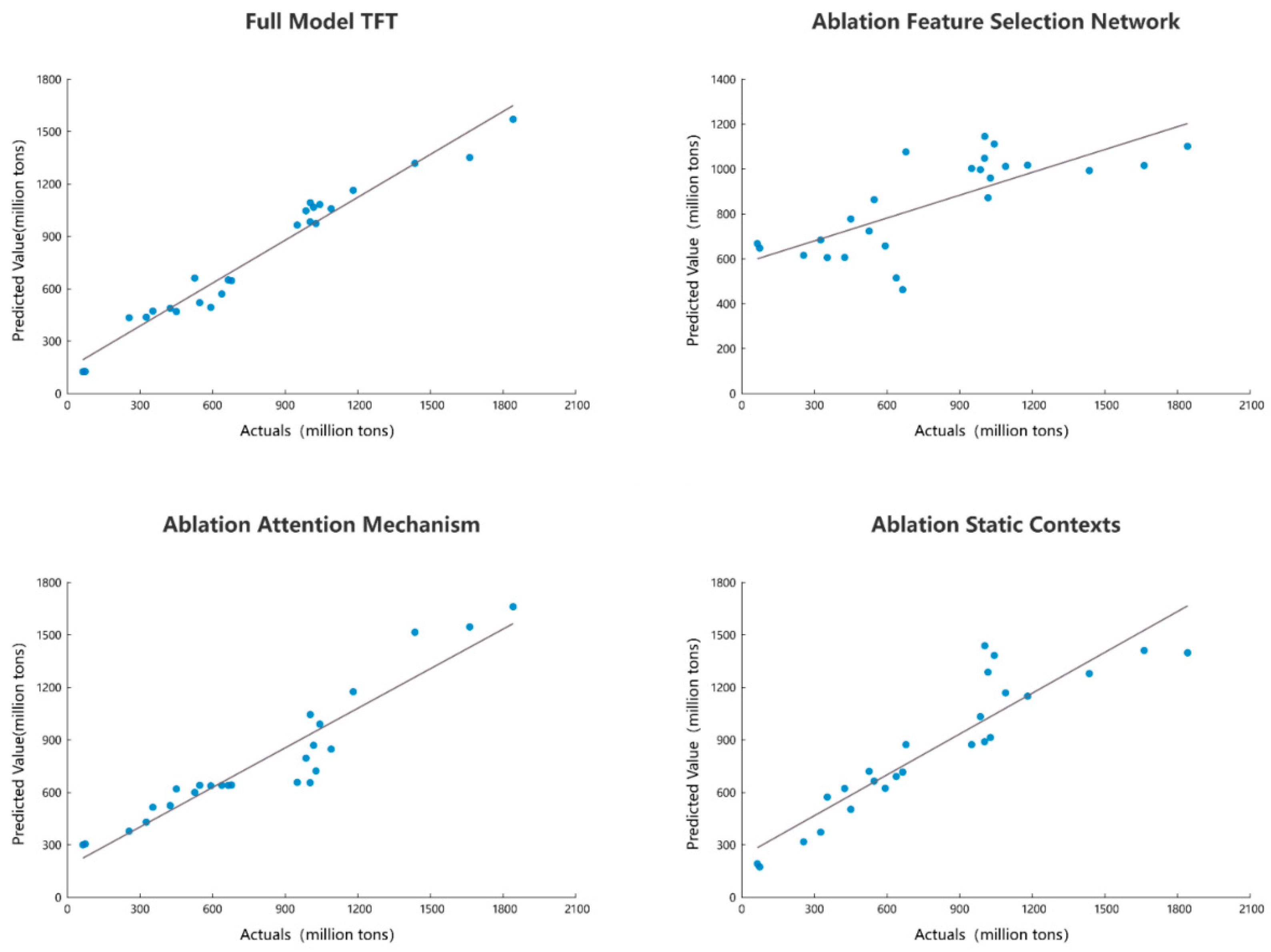
A comparative analysis of the prediction accuracy across different ablation models provides more intuitive and profound insights into the indispensable role of each component within the multivariate time-series forecasting system for the EEC system (see Figure 7). Regarding the overall characteristics of the prediction distribution, the scatter points of the full TFT model exhibit a tight clustering trend closely aligned with the diagonal line. This aligns with the quantitative results in Table 9, indicating that the full model can accurately capture the core patterns of the carbon emission time-series data, achieving a high degree of fit between predicted and actual values.

In contrast, the variant model with the feature selection network ablated shows a significantly more dispersed scatter distribution, with numerous predicted values deviating from the diagonal. A particularly severe underestimation occurs in the high carbon emission range (actual values between 1500–2000 million tons). This suggests that unfiltered multivariate inputs can overwhelm the model with irrelevant information, preventing it from distinguishing the primary and secondary influences of variables like energy consumption and economic growth on emissions, thereby weakening its ability to capture the core driving mechanisms. The variant model lacking the attention mechanism demonstrates a noticeable dispersion trend, with a higher number of outliers particularly in the low-to-medium emission range (actual values between 300–600 million tons). This confirms the critical value of the attention mechanism in time-series forecasting: without it, the model loses the capacity to discern varying influences across different historical time steps.

The variant with the static context encoder ablated exhibits a marked performance degradation. Its scatter points are extremely dispersed, even showing instances where predicted values are completely contrary to actual values. This conclusively proves the indispensability of static context. The static context encoder incorporates features such as inter-provincial geographical adjacency and energy resource endowments, which are key to explaining the spatial spillover effects of carbon emissions. Stripping away these static features leaves the model unable to establish a fundamental logical framework for carbon emissions, resulting in unfounded numerical fitting that ultimately leads to complete predictive failure.

Therefore, the complete TFT model is an excellent framework for studying the EEC system. The feature selection network, the attention mechanism, and the static context encoder are the three core components of the model. Their synergistic interaction serves as the core guarantee for the TFT model’s high-precision performance in carbon emission prediction.

4.3.3. Interpretability Analysis

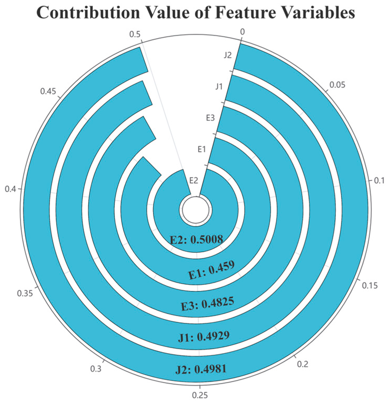
To further investigate the importance of each feature variable, this study visualizes their respective contributions to the model in Figure 8. In terms of feature importance weights, Total Energy Consumption (E2) ranks highest at 0.5008. This finding is highly consistent with the conclusions drawn from both the SDM (direct effect: 0.5050) and the system GMM model (coefficient: 0.1707), which also identified a significantly positive impact of total energy consumption on carbon emissions. Together, these results empirically confirm its absolute central role in driving carbon emissions within the Yellow River Basin. Furthermore, this outcome aligns with China’s current realities and policy context, particularly for provinces like Shanxi and Inner Mongolia in the Yellow River Basin—traditional energy and heavy industry bases whose economic growth models remain deeply intertwined with energy consumption.

The Proportion of Value-Added from the Secondary Industry (J2) and Regional GDP (J1), ranking second and third with weights of 0.4981 and 0.4929 respectively, jointly reveal the structural conflict between development and emissions. This reflects the persistent inertia of carbon emissions generated by the substantial share of the secondary industry amidst China’s pursuit of high-quality development.

The importance weights of Coal Consumption Share (E3) and Fossil Energy Production Share (E1) directly point to the carbon lock-in effect within the energy system. This is particularly relevant for the Yellow River Basin, a core national base for fossil energy production and a major high-carbon emission region, whose development has long been built upon a coal-centric energy system, resulting in a systemic carbon lock-in effect. This lock-in is manifested not only in the high dependence on coal mining and thermal power for energy supply but is also deeply embedded in the supporting heavy industrial structure, local fiscal systems, and even social stability frameworks. Together, these factors constitute a high-carbon development path dependency that is difficult to shift in the short term.

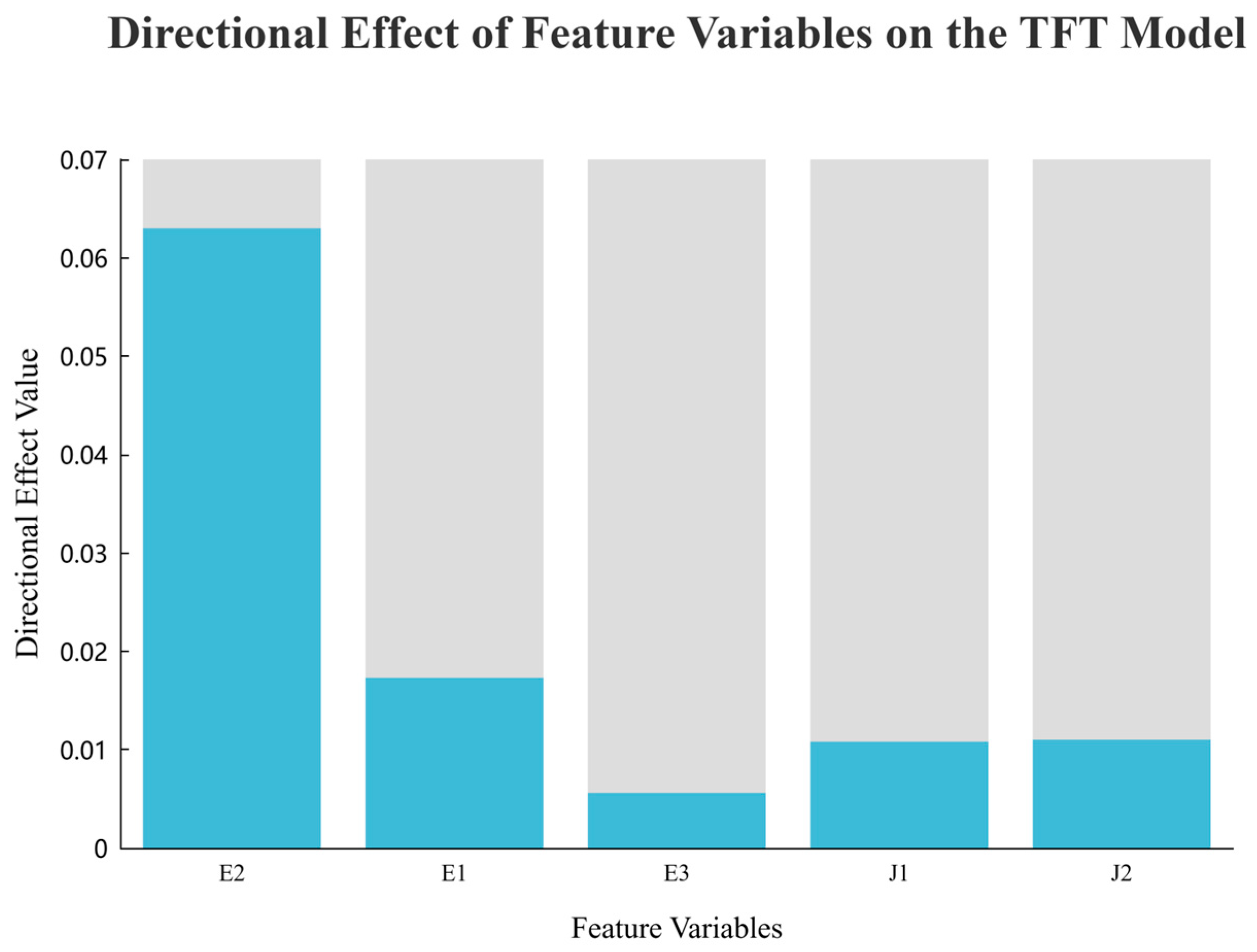
A directional effect plot of the feature variables provides an intuitive visualization of the positive or negative influence each variable exerts on the model (Figure 9). The results show that all key features exhibit a positive effect, meaning that each variable contributes to driving carbon emissions upwards. In this plot, the blue segments represent the specific values of the positive directional effect of each feature variable on the TFT model, quantifying the strength of each variable’s positive impact on carbon emissions, while the gray parts are merely background fill color with no practical data meaning. The positive effect of Total Energy Consumption (E2) is the most direct and robust. This indicates that any expansion of economic activity, unless accompanied by a significant improvement in energy efficiency, will lead to an increase in carbon emissions. The positive effect of the Proportion of Value-Added from the Secondary Industry (J2) highlights the carbon emission pressure stemming from a heavily industrialized economic structure. The positive effect of Regional GDP (J1) suggests that under the traditional growth paradigm, economic development and carbon emissions are not yet fully decoupled. The positive effect of Coal Consumption Share (E3) represents the most acute manifestation of the energy structure problem. It directly points to the core challenge of energy system transformation: how to safely and systematically reduce the proportion of coal in the primary energy mix. The positive effect of Fossil Energy Production Share (E1) reveals the importance of controlling carbon emissions from the supply side at its source.

In summary, the consistently positive effects of all feature variables collectively reveal that the Yellow River Basin remains deeply entrenched in the traditional development path dependence characterized by high energy consumption—high emissions. This fundamentally underscores both the urgency and the systemic challenge of promoting industrial restructuring and transitioning towards a cleaner energy system.

4.3.4. Model Prediction

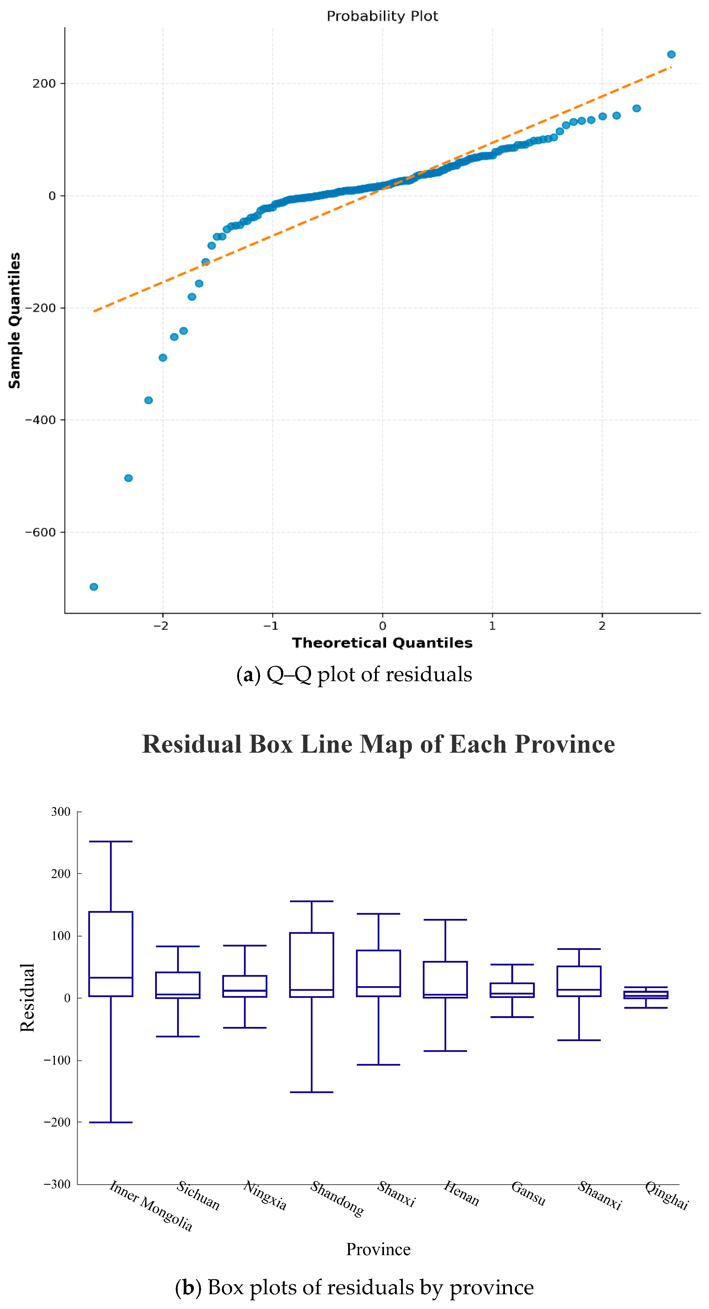
To further analyze the predictive accuracy of the model, this study examines the distribution of its residuals (Figure 10). The results show that the majority of the scatter points closely align with the orange reference line (the theoretical quantile line of a normal distribution, serving as the benchmark for normality) within the central region of the theoretical quantile range (−1 to 1). This indicates that the model’s predictions are well-concentrated for most samples. However, the points distributed at both ends, particularly those in the left tail, exhibit significant deviation from the reference line. This suggests that the residuals possess left-skewed and heavy-tailed characteristics, revealing a risk of model failure under specific scenarios. This finding is mutually consistent with the earlier conclusion that the model’s predictive performance deteriorates significantly at extremely low quantiles.

The box plots of provincial residuals visually present the distribution and dispersion of prediction errors across different provinces. Overall, the median residuals for most provinces are concentrated near zero, indicating no significant systematic bias in the model at the global level. However, there is marked heterogeneity in model performance across provinces. Provinces like Inner Mongolia and Shanxi, which are major energy producers and hubs for heavy industry, exhibit higher mean residuals and extremely large standard deviations. This implies that the model’s predictive stability is insufficient for these structurally complex provinces, which are highly susceptible to policy and economic shocks. In contrast, provinces such as Qinghai and Gansu show smaller residual fluctuations, indicating relatively more robust predictions.

In summary, the residual analysis confirms that the TFT model possesses good overall fitting capability. Simultaneously, it reveals the model’s vulnerability when dealing with extreme carbon emission pathways and regions characterized by high heterogeneity.

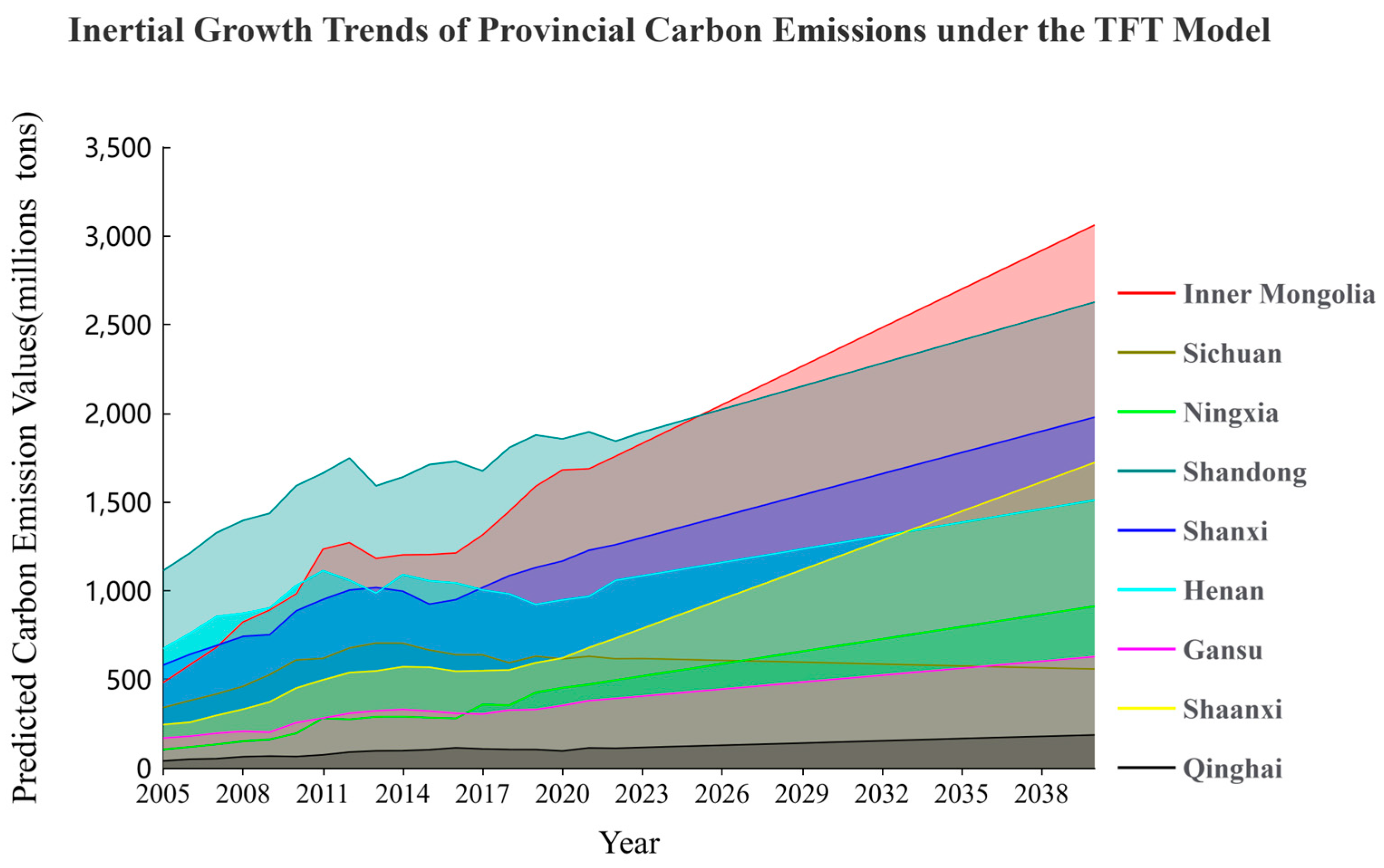
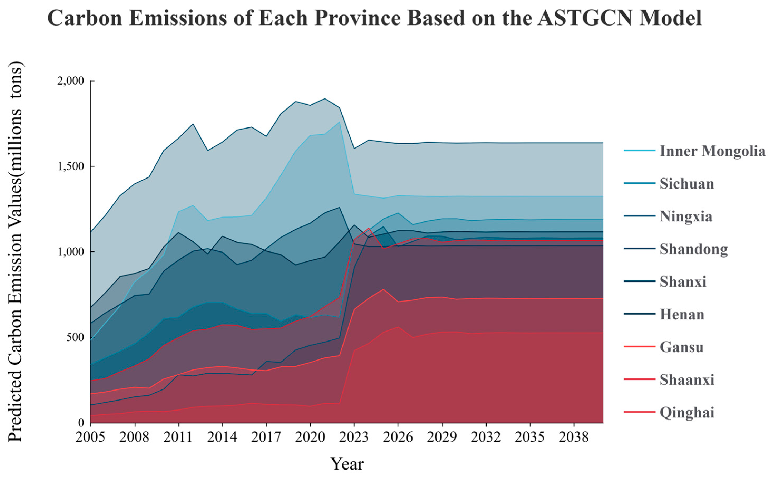
The TFT model forecasts future carbon emission trends from 2005 to 2040, with the period from 2005 to 2022 based on actual data (Figure 11). The results indicate that the total carbon emissions of the nine provinces in the Yellow River Basin are projected to continue growing, reaching levels significantly higher than those in 2022. This suggests the presence of a potent carbon lock-in effect and path dependence within the emission system primarily driven by energy consumption. This projection stands in tension with China’s national goal of achieving carbon peaking by 2030, manifesting in both temporal and magnitude dimensions. In terms of timing, carbon emissions in most provinces are projected to peak after 2030, failing to enter a declining trajectory before the target year. In terms of magnitude, the projected peak emission levels in high-emitting provinces such as Inner Mongolia, Shandong, and Shanxi are significantly higher, far exceeding the regional emission quotas aligned with the temperature control targets of the Paris Agreement. This finding points to a critical issue: under the current development pathway, the carbon peaking goal will not be achieved automatically; instead, it necessitates proactive and transformative policy and technological innovations to reverse this trend.

The predicted carbon emission pathways vary substantially across provinces. Inner Mongolia, as a national strategic energy base, exhibits the fastest projected growth rate and the largest emission volume, reflecting dual carbon lock-in pressures from both fossil energy production and consumption, necessitating systematic control measures at both ends of fossil energy supply and demand. Heavy industrial provinces such as Shandong and Shanxi show a pattern of sustained high-level growth, with significant spatial spillover effects from their industrial structures profoundly impacting regional emissions, requiring accelerated industrial structure upgrading and substantial reductions in total coal consumption. Sichuan is the only province among the nine predicted to show a declining trend within the forecast period. This can be attributed to its abundant hydropower resources, which have substantially reduced coal dependency, serving as evidence that energy structure transformation can drive decarbonization, with its clean energy advantage offering valuable insights for regional collaborative emission reduction. Conversely, the rapid growth projected for Ningxia serves as a warning that the relocation of industries and the development of emerging sectors must vigilantly guard against the formation of new high-carbon lock-in phenomena. The significant disparities among provinces underscore that carbon governance policies must be precisely implemented and tailored to local conditions.

Both the spatial econometric models and the TFT model consistently identify Total Energy Consumption and the Share of Coal Consumption as the most critical driving factors. This unequivocally determines that the primary direction for emission reduction in the Yellow River Basin must be the transformation of its energy system. The essential pathway involves controlling the total consumption of fossil fuels while ensuring energy security, and simultaneously accelerating the systematic replacement of coal with renewable energy sources such as wind and solar power.

4.4. ASTGCN Results Analysis

4.4.1. Impact of Network Depth on the Model

Although the TFT model excels in capturing the temporal dependencies, feature selection, and uncertainty quantification of the EEC system, and its prediction results clearly reveal the path dependence and regional heterogeneity of carbon emissions in the nine provinces of the Yellow River Basin, it remains fundamentally a time-series forecasting framework. As such, it struggles to directly capture the geographical spatial correlations and interactive influences of carbon emissions. Carbon emissions not only evolve over time but also exhibit significant spatial spillover and agglomeration characteristics. This is especially true for the spatial network formed among provinces in the Yellow River Basin due to factors like geographical adjacency and energy transfers, which further influence regional emission trends and mitigation effectiveness. Therefore, to more comprehensively and multidimensionally analyze the spatiotemporal synergistic mechanisms of carbon emissions and enhance the scientific basis for regional collaborative emission reduction strategies, it is necessary to introduce the ASTGCN model. ASTGCN can simultaneously model temporal dependencies and spatial correlations, capturing the dynamic influence relationships among provinces through graph structures. This addresses the spatial limitations of the TFT model, enabling truly integrated spatiotemporal predictive analysis.

To thoroughly investigate the architectural sensitivity of the ASTGCN model in capturing the spatiotemporal characteristics of carbon emissions in the Yellow River Basin and to optimize its predictive performance, this paper further analyzes the impact of network depth on model performance. As shown in

Table 10. Impact of the Number of Spatiotemporal Graph Convolutions on ASTGCN Performance.

Number of Temporal Convolution Layers	RMSE	R2
1	34.8666	0.7070
2	23.6266	0.8655
3	23.1832	0.8705
4	28.9356	0.7982
5	21.8181	0.8853

, as the network depth gradually increases from 1 to 5 layers, the model’s predictive performance exhibits pronounced fluctuations and stage-wise optimization characteristics. With a network depth of 1 layer, the model performance is relatively weak, with an RMSE of 34.8666 and an R² of 0.7070, indicating that shallow architectures struggle to adequately capture the complex spatiotemporal dependencies within the carbon emission system. When the depth increases to 2 layers, performance improves significantly, with the RMSE substantially decreasing to 23.6266 and R² rising to 0.8655, suggesting that an appropriate depth effectively enhances the model’s ability to extract spatiotemporal features. Further increasing the depth to 3 layers leads to a slight reduction in RMSE to 23.1832 and a marginal increase in R² to 0.8705, indicating that the model performance stabilizes with room for minor improvement. However, when the network depth reaches 4 layers, model performance notably declines, with RMSE rising to 28.9356 and R² dropping to 0.7982. This phenomenon may be attributed to training instability, gradient-related issues, or overfitting risks due to structural redundancy at this depth, demonstrating that more layers do not always lead to better performance and that increasing depth must be balanced with training stability. When the depth is further increased to 5 layers, model performance improves significantly again, achieving the lowest RMSE of 21.8181 and the highest R² of 0.8853, indicating that after overcoming the adjustment challenges at intermediate depths, a deeper network structure can leverage its stronger representational capacity to ultimately achieve a more precise characterization of the spatiotemporal evolution mechanisms of carbon emissions.

4.4.2. Role of the Adaptive Adjacency Matrix

Within the ASTGCN model, the adaptive adjacency matrix is a key component that dynamically captures the spatial correlations of carbon emissions among the nine provinces in the Yellow River Basin. Figure 12 presents the heatmap of the adaptive adjacency matrix for the ASTGCN model. Overall, its most prominent characteristics are a high degree of asymmetry and significant attention concentration. The asymmetry of the matrix indicates that the inter-provincial influences are directional. For instance, the influence weight from Gansu to Qinghai is significantly greater than the reverse, revealing potential dominant pathways for the spatial spillover of carbon emissions. Concurrently, the self-attention values on the matrix diagonal are generally prominent for provinces such as Shandong, Qinghai, and Shanxi. This empirically verifies that provincial carbon emissions exhibit strong path dependence and a carbon lock-in effect, meaning their future emission trends are largely dominated by their own historical states.

Further analysis of the significant association patterns in the results reveals several key spatial influence pathways. The strong linkage from Henan to Shandong stems not only from geographical proximity but also reflects a triple coupling of industry-energy-policy: As a supplier of raw materials and energy, Henan embeds embodied carbon into Shandong’s manufacturing output through industrial chains; the interconnected power grids of the two provinces mean Henan’s electricity generation mix directly affects Shandong’s consumption-side emissions; and differences in environmental regulations may potentially induce carbon leakage. Similarly, the linkages from Gansu to Qinghai, and from Shaanxi to Henan and Shanxi, collectively outline a regional carbon network structured around energy-rich areas and heavy industrial corridors. This network exhibits clear hierarchy and directionality, with some provinces acting as radiation sources dominating carbon flows, while others serve as receivers. Such structural characteristics indicate that regional carbon emissions are a complex spatial process resulting from the combined effects of economic-geographical division of labor, infrastructure connectivity, and policy gradients. Identifying its key hubs and transmission pathways is crucial for designing precise and coordinated emission reduction strategies. In contrast, provinces like Sichuan and Ningxia exhibit extremely low outward influence weights, suggesting they occupy relatively independent or peripheral positions within the spatial interaction network identified by the model.

The results of the adaptive adjacency matrix confirm that regional carbon emissions do not diffuse uniformly in space but rather follow several key directional pathways through influential hubs. The self-attention results for each province indicate that breaking the local carbon lock-in is fundamental to achieving emission reductions. Furthermore, the asymmetric association network revealed by the adaptive matrix provides a scientific basis for implementing differentiated and coordinated regional emission reduction strategies.

4.4.3. Model Prediction Results

The ASTGCN model projects carbon emissions from 2005 to 2040, with actual observed values used for the period 2005–2022. The prediction results of the ASTGCN model (Figure 13) reveal a carbon emission trajectory in the Yellow River Basin markedly different from simple temporal extrapolation. The core strength of the model lies in its spatiotemporal collaborative modeling capability. It not only accounts for the historical emission pathways of individual provinces but, more importantly, dynamically captures complex spatial spillover effects among provinces through graph convolutional networks and an adaptive adjacency matrix. These effects arise from geographical adjacency, energy flow, and economic linkages. From the specific data, ASTGCN projections indicate that carbon emissions in most provinces within the Yellow River Basin will peak between 2023 and 2026, followed by a slow decline or stabilization during a plateau phase. This pattern of slow reduction post-peak, which is also observed in traditional industrial provinces such as Shanxi and Henan, suggests that the model identifies a compelling and pulling mechanism driven by regional overall transition under spatial correlations, which pressures high-carbon provinces toward transformation. The asymmetric adaptive adjacency matrix reveals key influence pathways, such as Henan to Shandong and Gansu to Qinghai, implying that the clean transition of one province can generate positive emission-reduction spillover effects on linked provinces through channels like industrial supply chains and energy transmission networks.

Furthermore, the results indicate that achieving the Dual Carbon goals relies on an efficient regional collaborative system. The ASTGCN projected pathway suggests that if the Yellow River Basin can establish robust cross-provincial collaborative emission-reduction mechanisms, even energy-intensive provinces could achieve early peaking and rapid transformation while maintaining economic growth. The model’s projection of Sichuan’s consistently low emissions and its role as a clean energy hub further underscores the importance of closely integrating western clean energy bases with eastern load centers through infrastructure such as ultra-high-voltage power grids, thereby optimizing carbon flows at the regional scale.

The TFT model and the ASTGCN model have produced different results, with the core source of this divergence lying in the explicit modeling of spatial correlations in ASTGCN. TFT treats each province as an independent time series for prediction; while it excels in handling multivariate temporal dependencies, it fails to capture spatial interactions. In contrast, ASTGCN connects provinces through a graph structure, and its predictions inherently incorporate assumptions of spatial propagation effects. Overall, the difference between the predictions of TFT and ASTGCN essentially reflects the contrast between the inertia of isolated development and the potential of collaborative governance.

5. Conclusions

This study systematically deconstructs the driving mechanisms and future pathways of carbon emissions in the Yellow River Basin by integrating spatial econometric methods and machine learning models, arriving at the following core conclusions:

(1)

The energy system is the dominant driver of carbon emissions in the Yellow River Basin, exhibiting significant structural lock-in. Both total energy consumption and the proportion of coal consumption consistently show significant positive effects across all models, confirming the practical difficulty of fundamentally altering the coal-dominated energy structure in the short term. Accordingly, it is recommended that coal-consuming provinces such as Shandong and Henan establish binding coal consumption caps, accelerate coal-to-clean energy transitions, and implement regionally differentiated assessment mechanisms for energy structure transformation to break the system’s lock-in effect.

(2)

A preliminary decoupling trend is emerging between economic growth and carbon emissions, yet the industrial structure still exerts spatial spillover effects. The system GMM model reveals that, after controlling for endogeneity, the impact of regional GDP on carbon emissions turns negative, indicating initial success in achieving high-quality economic development. However, the significant spatial spillover effect of the secondary industry’s share suggests that inter-regional industrial linkages may still create synergistic emission pressures, necessitating overall emission reduction through industrial collaboration and the development of green supply chains.

(3)

Carbon emissions exhibit strong spatiotemporal dependence and regional heterogeneity. The SDM identifies high-high agglomeration characteristics in provinces like Shandong and Henan, while the ASTGCN model further delineates an asymmetric spatial influence network. This implies that emission reduction policies cannot be uniform but should be differentiated and coordinated based on the spatial correlation structure. It is therefore recommended that uniform policy approaches be replaced by regionally differentiated strategies based on spatial correlation structures. Agglomeration areas should adopt enhanced joint prevention and control measures, while transmission pathways should be clearly identified in radiating regions, combining differentiated targets with coordinated implementation.

(4)

Machine learning models provide higher-precision tools for carbon emission prediction and policy simulation. The TFT model excels at capturing multivariate nonlinear relationships. Its projections indicate that, under a business-as-usual scenario, carbon emissions in most provinces will continue to rise, presenting severe challenges for reaching peak emissions. In contrast, the ASTGCN model, by incorporating a spatial graph structure, predicts that with regional synergy, some provinces could achieve an earlier peak followed by a gradual decline, highlighting the crucial role of spatial coordination in emission reduction. A dynamic monitoring platform for spatially coordinated carbon peaking should be developed based on the ASTGCN model. Pilot programs for regional synergistic emission reduction should be launched in key provinces, integrating spatial correlation structures into the core framework of carbon peaking pathway planning.

6. Discussion

Building upon recent systemic assessments of the Yellow River Basin as an integrated socioeconomic-environmental system [47], this study systematically analyzes the driving mechanisms and evolutionary pathways of carbon emissions by integrating spatial econometric and machine learning methods. While yielding policy-relevant conclusions, several issues warrant further discussion, providing directions for future research.

(1)

Implications of Model Prediction Discrepancies: The TFT model, based on independent time-series predictions for each province, indicates sustained growth in carbon emissions for most provinces, reflecting the carbon lock-in effect of the current development pattern. In contrast, the ASTGCN model, by incorporating spatial correlations, predicts that regional synergy could facilitate an earlier peak and a steady decline for some provinces. This comparison highlights both the urgency and the potential of breaking administrative barriers and strengthening regional collaboration for achieving the Dual Carbon goals.

(2)

Specific Mechanisms of Spatial Synergy: The asymmetric spatial correlation network revealed by the ASTGCN model provides a structural foundation for spatial synergy. Its mechanisms are primarily manifested in energy complementarity, industrial linkages, and policy diffusion. For instance, hydropower transmission and industrial cooperation can effectively drive regional emission reduction. Future policies should leverage this network to implement differentiated and coordinated governance strategies, thereby transforming nodal advantages into synergistic network effects.

(3)

Transformational References: The Yellow River Basin and Comparable Global Regions: The transformation challenges of the Yellow River Basin share structural similarities with traditional industrial regions like Germany’s Ruhr area and the US Rust Belt. However, the Yellow River Basin uniquely plays a dual role as both an energy base and an ecological barrier. Its collaborative governance, therefore, requires greater emphasis on inter-provincial ecological compensation and benefit-sharing to balance the triple objectives of energy security, economic growth, and environmental protection. International experience suggests that successful basin-wide transformation relies on a multi-level governance system and continuous institutional innovation.

(4)

Extension of Existing Literature: This study aligns with most existing research regarding energy consumption as the core driver and the positive spatial correlation of carbon emissions. However, differing from some studies that posit a consistently positive relationship between economic growth and emissions, our system GMM analysis reveals a preliminary decoupling trend. This finding is consistent with recent trends of industrial structure optimization and energy efficiency improvement in the Yellow River Basin. Furthermore, compared to studies using only time-series models or traditional spatial econometric models, this research integrates the ASTGCN model to introduce a dynamic spatial graph structure into carbon emission prediction for the first time, uncovering an asymmetric spatial spillover network. This provides a more refined decision-making basis for regional collaborative emission reduction.

(5)

Policy Gap between Inertial and Target Trajectories: The TFT model projections show that under the current development pathway, carbon emissions in most provinces across the Yellow River Basin continue to rise, fundamentally deviating from China’s 2030 carbon peaking target and the temperature control goals of the Paris Agreement. This gap reflects a regional manifestation of the structural contradiction between the high-carbon development model and global climate governance requirements. Significant discrepancies exist between the model-projected inertial trajectory and the normative pathway demanded by global targets across three dimensions: peaking timing, peak levels, and post-peak decline rates. To achieve convergence from the inertial to the target trajectory, systematic and differentiated policy interventions are required across three fronts: energy structure optimization, industrial upgrading, and cross-regional collaborative governance, thereby translating the identified policy gaps into actionable emission reduction pathways.

(6)

Research Limitations and Future Directions: This study also has several limitations. First, the predictive performance of the TFT model decreases under extreme low-carbon scenarios, suggesting a need for future work to integrate scenario analysis or reinforcement learning to enhance its ability to capture structural shifts. Second, the variable system could be expanded to include negative inhibitory indicators such as renewable energy consumption and carbon sink capacity, providing a more comprehensive reflection of system dynamics. Third, data timeliness and spatial resolution require improvement; future research could incorporate higher-frequency, finer-grained data to support dynamic policy simulation. Finally, as carbon emission pathways are subject to multiple uncertainties, subsequent studies could integrate stochastic optimization and risk assessment to enhance the robustness and adaptability of policy recommendations.

References

1. Millinger, M.; Hedenus, F.; Zeyen, E.; Neumann, F.; Reichenberg, L.; Berndes, G. Diversity of biomass usage pathways to achieve emissions targets in the European energy system. Nat. Energy 2025, 10, 226–242. [Google Scholar] [CrossRef] [Scilit]
2. Yakymchuk, A.; Rataj, M.A. Economic Analysis of Fossil CO2 Emissions: A European Perspective on Sustainable Development. Energies 2025, 18, 2106. [Google Scholar] [CrossRef] [Scilit]
3. Secretariat, U. Compilation and Synthesis of Fifth Biennial Reports of Parties Included in Annex I to the Convention; United Nations: New York, NY, USA, 2023. [Google Scholar]
4. den Elzen, M.G.J.; Dafnomilis, I.; Nascimento, L.; Beusen, A.; Forsell, N.; Gubbels, J.; Harmsen, M.; Hooijschuur, E.; Araujo Gutiérrez, Z.; Kuramochi, T. Uncertainties around net-zero climate targets have major impact on greenhouse gas emissions projections. Ann. N. Y. Acad. Sci. 2025, 1544, 209–222. [Google Scholar] [CrossRef] [Scilit]
5. Friedlingstein, P.; Le Quéré, C.; O’Sullivan, M.; Hauck, J.; Landschützer, P.; Luijkx, I.T.; Li, H.; van der Woude, A.; Schwingshackl, C.; Pongratz, J.; et al. Emerging climate impact on carbon sinks in a consolidated carbon budget. Nature 2025, 649, 98–103. [Google Scholar] [CrossRef] [Scilit]
6. Costantini, L.; Laio, F.; Mariani, M.S.; Ridolfi, L.; Sciarra, C. Forecasting national CO2 emissions worldwide. Sci. Rep. 2024, 14, 22438. [Google Scholar] [CrossRef] [Scilit]
7. Friedlingstein, P.; Artaxo, P.; Gallego-Sala, A.V.; Jia, G.; Jones, C.D.; Kawamiya, M.; Loisel, J.; Loutre, M.-F.; Rehfeld, K.; Rovere, A.; et al. Earth system responses to different levels of greenhouse gas emissions mitigation. Front. Clim. 2024, 6, 1480208. [Google Scholar] [CrossRef] [Scilit]
8. Cantone, B.; Evans, D.; Reeson, A. The effect of carbon price on low carbon innovation. Sci. Rep. 2023, 13, 9525. [Google Scholar] [CrossRef] [Scilit]
9. Tong, D.; Zhang, Q.; Zheng, Y.; Caldeira, K.; Shearer, C.; Hong, C.; Qin, Y.; Davis, S.J. Committed emissions from existing energy infrastructure jeopardize 1.5 °C climate target. Nature 2019, 572, 373–377. [Google Scholar] [CrossRef] [Scilit] [PubMed]
10. Azevedo, I.; Bataille, C.; Bistline, J.; Clarke, L.; Davis, S. Net-zero emissions energy systems: What we know and do not know. Energy Clim. Change 2021, 2, 100049. [Google Scholar] [CrossRef] [Scilit]
11. Kiarsi, M.; Masoudi, N. Optimal environmental policy and distortionary fiscal policy interactions: A DSGE perspective. Econ. Model. 2025, 147, 107037. [Google Scholar] [CrossRef] [Scilit]
12. Chen, D.; Li, S. Exploring the pathway to carbon neutrality in China based on a dynamic spatial Durbin quantile regression model. Sci. Rep. 2025, 15, 17442. [Google Scholar] [CrossRef] [Scilit]
13. Li, K.; Wang, H.; Xie, X. Mechanism and spatial spillover effect of the digital economy on urban carbon Productivity: Evidence from 271 prefecture-level cities in China. J. Environ. Manag. 2025, 382, 125435. [Google Scholar] [CrossRef] [Scilit] [PubMed]
14. Su, X.; Qiao, R.; Xu, S. Impact of green finance on carbon emissions and spatial spillover effects: Empirical evidence from China. J. Clean. Prod. 2024, 45, 142362. [Google Scholar] [CrossRef] [Scilit]
15. You, W.; Lv, Z. Spillover effects of economic globalization on CO2 emissions: A spatial panel approach. Energy Econ. 2018, 73, 248–257. [Google Scholar] [CrossRef] [Scilit]
16. Ndayambaje, J.d.D.; Yang, L.; Samuel, A.O.; Gakuru, E. The role of climate policies in alleviating global energy poverty. Evidence from system GMM analysis. Energy 2025, 330, 6990. [Google Scholar] [CrossRef] [Scilit]
17. Koç, Ş.; Uctu, R.; Essop, H.; Mercan, B. The impact of innovation on economic growth: A dynamic panel data analysis using system GMM approach. Int. J. Innov. Stud. 2026, 10, 20–30. [Google Scholar] [CrossRef] [Scilit]
18. Lai, L.; Zhang, S.; Li, L.; Zhu, D. Effects of human inequality and urbanization on ecological well-being performance: A System-GMM analysis. Heliyon 2024, 10, e34040. [Google Scholar] [CrossRef] [Scilit]
19. Zhang, Z.; Hua, Z.; He, Z.; Wei, X.; Sun, H. The impact of local government attention on green total factor productivity: An empirical study based on System GMM dynamic panel model. J. Clean. Prod. 2024, 458, 142275. [Google Scholar] [CrossRef] [Scilit]
20. Lim, B.; Arık, S.Ö.; Loeff, N.; Pfister, T. Temporal Fusion Transformers for interpretable multi-horizon time series forecasting. Int. J. Forecast. 2021, 37, 1748–1764. [Google Scholar] [CrossRef] [Scilit]
21. Chan, J.W.; Yeo, C.K. A Transformer based approach to electricity load forecasting. Electr. J. 2024, 37, 107370. [Google Scholar] [CrossRef] [Scilit]
22. Dai, T.-Y.; Niyogi, D.; Nagy, Z. CityTFT: A temporal fusion transformer-based surrogate model for urban building energy modeling. Appl. Energy 2025, 389, 125712. [Google Scholar] [CrossRef] [Scilit]
23. Suresh, C.V.; Bhukya, M.N.; Arya, Y. Environmental air pollution forecasting using sensor networks, edge computing, and temporal fusion transformers. Eng. Appl. Artif. Intell. 2026, 167, 113961. [Google Scholar] [CrossRef] [Scilit]
24. Xiao, L.; Wang, Y.; Meng, A.; Tan, Z.; Chen, S.; Song, S.; Yin, H.; Luo, J. Power prediction methods for offshore wind farm clusters: Interpretable ASTGCN based on wind speed delay perception and spatial feature fusion. Energy 2025, 341, 139345. [Google Scholar] [CrossRef] [Scilit]
25. Liu, X.; Lu, J.; Chen, X.; Fong, Y.H.C.; Ma, X.; Zhang, F. Attention based spatio-temporal graph convolutional network with focal loss for crash risk evaluation on urban road traffic network based on multi-source risks. Accid. Anal. Prev. 2023, 192, 107262. [Google Scholar] [CrossRef] [Scilit]
26. Wen, S.; Zhang, W.; Zhou, N.; Yuan, L. Adaptive spatio-temporal graph convolutional network for rapid indoor temperature field prediction with limited sensors. Build. Environ. 2025, 283, 113346. [Google Scholar] [CrossRef] [Scilit]
27. Wang, W.; Luo, Y.; Jiang, Z.; Zhou, J.; Jia, P. A deep learning framework for global transportation energy carbon emission forecasting: Integrating generative pre-trained transformer with multi-scale feature analysis. Energy 2025, 338, 138586. [Google Scholar] [CrossRef] [Scilit]
28. Zhao, W.; Jiang, Y. The Spatiotemporal Prediction Model of Urban Carbon Emissions Based on Graph Neural Networks. Int. J. Inf. Technol. Syst. Approach 2025, 18, 1–17. [Google Scholar] [CrossRef] [Scilit]
29. Liu, B.; Chang, H.; Li, Y.; Zhao, Y. Carbon emissions predicting and decoupling analysis based on the PSO-ELM combined prediction model: Evidence from Chongqing Municipality, China. Environ. Sci. Pollut. Res. 2023, 30, 78849–78864. [Google Scholar] [CrossRef] [Scilit] [PubMed]
30. Begum, A.M.; Mobin, M.A. A machine learning approach to carbon emissions prediction of the top eleven emitters by 2030 and their prospects for meeting Paris agreement targets. Sci. Rep. 2025, 15, 19469. [Google Scholar] [CrossRef] [Scilit]
31. Khajavi, H.; Rastgoo, A. Predicting the carbon dioxide emission caused by road transport using a Random Forest (RF) model combined by Meta-Heuristic Algorithms. Sustain. Cities Soc. 2023, 93, 104503. [Google Scholar] [CrossRef] [Scilit]
32. Zhang, P. Enhanced short-term carbon emission forecasting via hybrid decomposition-denoising modeling. Sci. Rep. 2025, 15, 36211. [Google Scholar] [CrossRef] [Scilit] [PubMed]
33. Šimić, G.; Radovanović, M.; Filipović, S. Assessment of the decarbonization efficiency in the European Union: Machine learning approach. Energy Sustain. Soc. 2025, 15, 52. [Google Scholar] [CrossRef] [Scilit]
34. Li, Q.; Chen, J. Temporal–spatial characteristics of carbon emissions and low-carbon efficiency of regional energy consumption: A case study of Beijing-Tianjin-Hebei, Yangtze River Delta and Sichuan-Chongqing regions. Ecol. Indic. 2025, 179, 114285. [Google Scholar] [CrossRef] [Scilit]
35. Xie, P.; Shu, Y.; Sun, F.; Li, P. Decoupling economic development from carbon emissions: Insights from Chinese provinces. Energy 2024, 308, 133008. [Google Scholar] [CrossRef] [Scilit]
36. Pierre Friedlingstein, M.O.S.; Jones, M.W.; Andrew, R.M.; Hauck, J.; Landschützer, P.; Le Quéré, C.; Li, H.; Luijkx, I.T.; Olsen, A.; Peters, G.P.; et al. Global Carbon Budget 2024. ESSD 2025, 17, 965–1039. [Google Scholar]
37. Elhorst, J.P. Spatial Econometrics; Springer: New York, NY, USA, 2014. [Google Scholar]
38. Li, Y.; Yang, X.; Ma, S. The Efficiency Measurement and Spatial Spillover Effect of Green Technology Innovation in Chinese Industrial Enterprises. Sustainability 2025, 17, 3162. [Google Scholar] [CrossRef] [Scilit]
39. Liu, Y.; Xiao, H.; Zikhali, P.; Lv, Y. Carbon Emissions in China: A Spatial Econometric Analysis at the Regional Level. Sustainability 2014, 6, 6005–6023. [Google Scholar] [CrossRef] [Scilit]
40. Guan, Y.; Shan, Y.; Huang, Q.; Chen, H.; Wang, D.; Hubacek, K. Assessment to China’s Recent Emission Pattern Shifts. Earth’s Future 2021, 9, e2021EF002241. [Google Scholar] [CrossRef] [Scilit]
41. Shan, Y.; Guan, D.; Zheng, H.; Ou, J.; Li, Y.; Meng, J.; Mi, Z.; Liu, Z.; Zhang, Q. China CO2 emission accounts 1997–2015. Sci. Data 2018, 5, 170201. [Google Scholar] [CrossRef] [Scilit] [PubMed]
42. Shan, Y.; Huang, Q.; Guan, D.; Hubacek, K. China CO2 emission accounts 2016–2017. Sci. Data 2020, 7, 54. [Google Scholar] [CrossRef] [Scilit]
43. Shan, Y.; Liu, J.; Liu, Z.; Xu, X.; Shao, S.; Wang, P.; Guan, D. New provincial CO2 emission inventories in China based on apparent energy consumption data and updated emission factors. Appl. Energy 2016, 184, 742–750. [Google Scholar] [CrossRef] [Scilit]
44. Xu, J.; Guan, Y.; Oldfield, J.; Guan, D.; Shan, Y. China carbon emission accounts 2020-2021. Appl. Energy 2024, 360, 122837. [Google Scholar] [CrossRef] [Scilit]
45. Huang, Y.; Hong, T.; Ma, T. Urban network externalities, agglomeration economies and urban economic growth. Cities 2020, 107, 102882. [Google Scholar] [CrossRef] [Scilit]
46. James LeSage, R.K.P. Introduction to Spatial Econometrics; Chapman and Hall/CRC: New York, NY, USA, 2009. [Google Scholar]
47. Zhang, C.; Wei, Y.; Zhao, X.; Hu, J. Assessment and enhancement pathways of the water-energy-food-economy-ecosystem nexus in China’s yellow river basin. Energy 2025, 316, 134492. [Google Scholar] [CrossRef] [Scilit]
Figure 1. Map of the Yellow River Basin.
Energies 19 01950 g001
Figure 2. TFT Model Structural Framework.
Energies 19 01950 g002
Figure 3. ASTGCN Model Structure Diagram.
Energies 19 01950 g003
Figure 4. Results of the Local Moran’s I Test.
Energies 19 01950 g004
Figure 5. Comparison of Different Quantile Settings for the TFT Model.
Energies 19 01950 g005
Figure 6. Threshold Comparison.
Energies 19 01950 g006
Figure 7. Comparison of Prediction Accuracy in Ablation Experiments.
Energies 19 01950 g007
Figure 8. Feature Contribution Values.
Energies 19 01950 g008
Figure 9. Directional Effects of Feature Variables.
Energies 19 01950 g009
Figure 10. Q–Q Plot of Residuals and Box Plots of Residuals by Province.
Energies 19 01950 g010
Figure 11. Provincial Carbon Emission Predictions Based on the TFT Model.
Energies 19 01950 g011
Figure 12. Heatmap of the Adaptive Adjacency Matrix in the ASTGCN Model.
Energies 19 01950 g012
Figure 13. Carbon Emission Prediction Results Based on the ASTGCN Model.
Energies 19 01950 g013