An Energy Flow Control Strategy for Residential Buildings with Electric Vehicles as Storage and PV Systems

Abstract

Modern power systems increasingly integrate renewable energy sources (RESs), electric mobility, and dynamic market participation. Dynamic electricity pricing, reflecting real-time market conditions, is increasingly important for prosumers worldwide, enabling flexible and efficient energy management. The growing adoption of electric vehicles (EVs) and bidirectional charging technologies (V2G, V2H) allows EVs to act as mobile battery energy storage systems (mBESSs). This study presents a Python 3.11-based application for simulating and analyzing energy flows in residential systems with photovoltaic (PV) installations, EVs acting as mBESS, and optional stationary battery energy storage systems (BESSs), using real 2024 data on consumption, PV production, and market prices. The energy management system (EMS) employs a rule-based algorithm to optimize energy use and economic benefits, adjusting dispatch between PV systems, the grid, mBESSs, and BESSs based on price coefficients $\alpha$ and $\beta$. Simulation scenarios were developed based on two EV availability patterns: Profile 1, representing users unavailable during standard working hours, and Profile 2, representing users with intermittent availability for brief excursions. The results demonstrate substantial electricity cost reductions: For a Nissan Leaf e+ with Profile 1, annual costs decrease by approximately 20% compared to a system without EVs. With PV generation and Profile 2, costs drop by 57% relative to the baseline, while adding a stationary BESS further reduces costs by nearly 95%. It should be noted that the results were obtained assuming zero energy costs for propulsion. Therefore, the economic benefits reported here represent an upper-bound estimate and would be lower under real-world driving conditions. These findings highlight that coordinated EMS operation with EVs as mBESSs, supported by optional BESSs, can maximize economic performance and provide prosumers with a practical framework for flexible and efficient energy management.

1. Introduction

Modern power systems are undergoing a dynamic transformation driven by the increasing share of renewable energy sources (RESs), the rapid development of electromobility, and the emergence of new models of end-user participation in the energy market. A central component of the ongoing energy transition is the implementation of dynamic electricity pricing, which accurately mirrors the temporal variations in supply and demand. Dynamic electricity prices are particularly important in the context of prosumers—consumers who simultaneously act as producers of energy, most commonly equipped with photovoltaic (PV) installations, battery energy storage systems (BESSs) or electric vehicles (EVs) with Vehicle-to-Home (V2H) or Vehicle-to-Grid (V2G) capabilities. Pricing mechanisms based on wholesale market values enable effective energy management by supporting demand-side flexibility (DSF). DSF refers to the ability of consumers and prosumers to respond to price signals by adjusting their energy consumption or generation patterns.

In many European countries, dynamic electricity billing models are becoming increasingly common among households [1]. In the Scandinavian region, such models operate under Nord Pool, the main electricity exchange, which facilitates trading on both the Day-Ahead Market (DAM) and the Intraday Market (IM). This region does not have its own national exchanges. Instead, all trading is centralized via Nord Pool. The prices in each individual zone are set according to the available transmission capacity in the network and the balance between supply and demand. The German electricity market operates as a single price zone and is managed by EPEX SPOT, where electricity prices are established for both the DAM and IM. Under the Renewable Energy Sources Act, since 2023, suppliers serving more than 100,000 customers have been required to offer hourly dynamic tariffs. In the United Kingdom, energy trading is conducted primarily through the UK Power Exchange and through bilateral contracts between market participants. Here, dynamic hourly tariffs are also available to end users, such as Time-of-Use tariffs, which reflect variable electricity prices depending on the time of day. In Poland, electricity distribution companies serving at least 200,000 customers are required to offer dynamic tariff groups. Electricity prices are determined on the Polish Power Exchange (TGE) within the DAM. The Polish electricity market operates under Multi-NEMO Arrangements, which means that market participants can submit orders through exchanges such as EPEX SPOT and Nord Pool, while auction results are integrated within the Single Day-Ahead Coupling mechanism. Within the DAM, hourly and block contracts are available—including base, peak, and off-peak products. The primary reference point for prices in the DAM is Fixing I, the main trading session during which purchase and sale orders are matched to determine the market equilibrium price. Price variations are reflected by six price indices, each corresponding to a specific day and delivery period. Dynamic electricity pricing and the development of cross-border energy markets promote increasingly flexible energy use by end consumers and prosumers. The growing availability of hourly tariffs and the possibility of integration with energy storage systems and EVs create new opportunities to optimize energy consumption and manage costs. An expanding segment of the automotive market consists of EVs, whose share in Europe continues to grow each year. In 2023, hybrid electric vehicles without external charging capability (HEVs) accounted for 25.8%, while battery electric vehicles (BEVs) and plug-in hybrid electric vehicles (PHEVs) represented 22.3%. In 2024, the sales share of BEVs and PHEVs decreased to 20.7%, while HEVs increased to 30.9%. This indicates that more than half of all vehicles sold in 2024 were electrically powered. By May 2025, the total share of electric-powered passenger cars reached 58.7%, confirming the year-over-year growth of EVs sales on the European market [2].

EVs are becoming not only a means of transportation but also an active component of the power system. An increasing number of models support bidirectional charging, allowing energy to flow not only from the grid to the EV but also from the EV back to the home energy system (V2H) or the power grid (V2G). The key enabling element of this functionality is the bidirectional charger, which, in addition to standard charging, can operate in inverter mode. Consequently, EVs can act as a mobile energy storage system (mBESS), which can be used in multiple ways, e.g., to supply energy to a building during high-price periods or to inject energy into the grid during times of deficit. The advancement of bidirectional charging technologies supports the integration of EVs into the energy market, enhancing their role as active participants in the power system, particularly in the context of the increasing share and variability of RESs [3].

In facilities equipped with PV installations and BESSs or mBESSs, the Energy Management System (EMS) plays a central role in realizing the full economic and technical potential of the system. Based on data from energy meters, PV production, consumption forecasts, and market information (e.g., electricity prices), the EMS can make informed decisions regarding charging and discharging cycles and manage the operation of the bidirectional EV charger. Acting as the “brain” of the integrated energy system, the EMS aims, depending on the algorithm implemented, to maximize overall economic efficiency [4]. For monetary calculations, all costs in EUR are converted from PLN using the exchange rate of 1 EUR = 4.273 PLN (rate as of 31.12.2024).

This work makes three main contributions. First, it proposes a transparent, rule-based EMS for residential systems with PV systems, EVs acting as mBESSs, and an optional stationary BESS, in which charging and discharging decisions are governed by two constant price coefficients $\alpha$ and $\beta$ applied to a dynamic moving average of hourly DAM prices. This simple, parameterized structure avoids forecasting modules and computationally intensive optimization while still exploiting short-term price fluctuations through market-linked thresholds. Second, the EMS is validated over a full year using real 2024 data from a Polish single-family house-measured consumption, PV generation and TGE DAM prices under actual G11 and G11f tariffs—providing an empirically grounded assessment of economic performance in a specific market environment. Third, a Python/Streamlit application is delivered that lets users upload their own profiles, configure system parameters, and explore the impact of different EV, PV and BESS configurations and price coefficients on energy flows and costs, offering a practical decision-support tool for prosumers.

The structure of this article is as follows. Section 2 presents the motivation and research objectives related to the development and validation of an energy flow control algorithm for a system integrating an EV as an energy storage component with a PV installation. Section 3 provides a comprehensive literature review discussing recent advances in bidirectional EV charging technologies. Section 4 presents the proposed methodology, including the rule-based energy management algorithm, its mathematical formulation, and the structure of the developed simulation application. Section 5 discusses the simulation results, including the impact of different system configurations, EV availability profiles, and price coefficients on economic performance, along with a detailed economic analysis. Finally, Section 6 summarizes the main findings, highlights the key contributions of the study, and outlines directions for future research.

2. Motivation

In recent years, the European Union (EU), along with numerous other regions around the world, has seen a marked increase in the proportion of RESs in electricity generation. In 2024, RESs accounted for roughly 47% of total net electricity production in the EU [5]. A large fraction of this share originated from variable weather-dependent technologies: wind power provided 17.8% and solar energy 9.25%, jointly exceeding 27% of total output from variable RESs. Because these technologies are characterized by fluctuating and difficult-to-forecast generation patterns, their increasing penetration creates significant challenges for power system balancing and energy storage. Under these circumstances, the demand for distributed energy storage systems that can locally match energy generation and consumption is continuously increasing. In this context, EVs can play a particularly significant role as they are able to charge during times of excess generation and feed energy back into the grid during peak demand periods by means of bidirectional charging technologies.

Employing EVs as mBESSs requires the design of an EMS that can effectively manage charging and discharging operations based on the availability of renewable energy and the prevailing electricity prices. The functional specifications for such a system include the following:

• A dynamic control algorithm based on electricity prices;
• An algorithm incorporating multiple energy assets, such as an EV, BESS, PV installation, building load profile, and variable electricity prices;
• The ability to perform simulations using diverse input datasets;
• The development of a computational application that implements the proposed algorithm, acting as a decision-support environment (reality simulator) for end users.

The development of the computational application is based on the following assumptions:

• A simplified battery charging model based on an hourly energy balance, without detailed electrochemical characteristics;
• The use of real energy consumption and PV generation profiles obtained from experimental facilities;
• The use of historical electricity prices from the SPOT market of TGE augmented with a comprehensive financial structure—including variable distribution fees, transmission costs, and taxes—to reflect the actual economic conditions of a household bill;
• The execution of multi-dimensional scenario analysis, enabling the user to isolate and evaluate the economic impact of individual system components (PV, stationary BESSs, and mBESSs) across various configurations (e.g., with/without PV, with/without V2H). The simulator accounts for real-world operational constraints, such as EV availability windows, and diverse electricity tariff structures.

This methodology enables the evaluation of both the economic gains and the practical feasibility of using EVs as mBESSs within a local energy system.

3. State of the Art

Research on the deployment of bidirectional charging technologies, which includes applications such as V2G and V2H, has attracted growing interest from the scientific community, policy makers, and the automotive and energy sectors. The increasing penetration of RESs in electricity generation and the increasing demand for flexibility in power systems provide favorable conditions for the use of these technologies as instruments to couple renewable energy with the transport and end-use sectors [6].

Research on bidirectional charging is being carried out from diverse perspectives and across a wide range of use cases, such as public parking facilities with integrated charging infrastructure, the coupling of RESs at charging stations and community-oriented energy concepts (Community-V2G-Power), in which EVs play an active role in stabilizing local energy systems [7]. A growing number of end users feed electricity back into the grid and thus evolve into prosumers. For these prosumers, connecting EVs to the power grid enables active participation in electricity markets, greater energy autonomy, and potential economic gains, mainly through price arbitrage, the provision of auxiliary services (e.g., frequency regulation), and the use of dynamic electricity tariffs [8].

The analyses show that the economic value realized from V2G is strongly influenced by the specific design of the market, the prevailing electricity prices, the costs of battery degradation and the intensity of the charge–discharge cycle [9]. For EV users, battery degradation remains the dominant concern as it decreases usable capacity and shortens overall service life [10,11]. Research employing multi-objective optimization frameworks for V2G scheduling that explicitly account for cell aging indicates that carefully designed operational strategies can curb negative degradation effects while preserving economic feasibility [12,13]. However, despite these possible financial advantages and the prospect of reduced degradation, the overall willingness of EV users to adopt V2G remains relatively low [14].

Fostering user trust requires transparent billing schemes, targeted educational measures, and the incorporation of user-specific preferences—such as preferred departure times or minimum state-of-charge thresholds—into optimization frameworks [15,16]. Emerging economic evaluation approaches, such as the BSTP Framework [7], explicitly position prosumers as central stakeholders within the V2G ecosystem and offer a structured way to reassess the economic viability of V2G across different market designs and business models. However, such comprehensive, optimization-oriented frameworks typically require detailed input data, advanced modeling capabilities, and substantial computational resources, which limits their direct applicability in lightweight, real-time EMS implementations at the household scale. The authors stress that a large part of existing research relies on large-scale theoretical formulations that are seldom empirically validated, constraining the assessment of tangible benefits from the end-user point of view. From the user perspective, aspects of system control and interface design are also crucial [17,18]. As a result, recent solutions increasingly employ intelligent scheduling and menu-based pricing mechanisms to streamline decision-making and strengthen user participation.

Conceptual studies and pilot implementations of V2G and V2H technologies are becoming increasingly important as they allow for a practical assessment of their advantages and drawbacks, as well as their interaction with energy markets and existing grid infrastructure. The role of EVs as distributed energy resources (DERs) that can enhance grid stability can only be fully exploited if the social dimensions and user behavior are taken into account properly [19]. Current pilot initiatives encompass both single EVs and aggregated EV fleets operating in V2G mode, requiring suitable strategies to manage charging and discharging processes [20].

Pilot projects are underway in several countries, including Japan [21], the Netherlands [15], the United Kingdom [22], the United States [23], South Korea [24], and Australia [25]. These initiatives primarily aim to evaluate bidirectional charging technologies, their integration with local energy systems, and their effects on battery degradation and user-level economics. From the grid’s perspective, it is crucial to develop V2G implementation frameworks tailored to specific market environments, such as the Polish context [26]. In addition, simulation models have been proposed to support the integration of EVs into energy markets, accounting for both operational behavior and economic performance [27].

The broad deployment of bidirectional charging technologies depends on adherence to established technical standards and to national as well as international regulatory frameworks. In this context, communication protocols such as ISO 15118 [28], CHAdeMO 2.0, and CCS with V2G extensions serve as a fundamental basis for ensuring interoperability between the charging infrastructure and EVs. Their implementation necessitates a harmonized framework for certification and communication among the EV, the charging station, and the system operator, alongside regulatory provisions for both infrastructure and bidirectional EVs [29]. At the same time, successful integration of EVs with V2G and V2H functions remains a multidimensional challenge that not only spans these technical, standardization, and compliance aspects but also involves social and behavioral determinants of user adoption; consequently, EMSs must incorporate individual user preferences, such as desired charging times and comfort requirements, in order to fully exploit the capability of EVs as flexible energy resources.

Commercially available AC and DC bidirectional chargers that enable energy exchange are already on the market, and wireless bidirectional charging technologies are under active development [30]. Automakers are releasing EV models that support the V2G and V2H functionalities, while ongoing research investigates converter topologies and control strategies that improve energy management in bidirectional architectures [31]. Despite extensive studies on how different charging strategies affect battery lifetime, the technical coupling of EVs with the power grid must be supported by advanced diagnostic methods, rigorous quality control, and adaptive charging management systems tailored to real-world usage patterns and the specific energy profiles of households and EV fleets.

Table 1. Comparison of the proposed rule-based EMS with optimization and prediction-based EMS approaches.

Feature/Aspect	Optimization-Based EMS	Prediction-Based EMS	Proposed Rule-Based EMS
Decision strategy	Multi-objective mathematical optimization with explicit technical and economic constraints [32,33]	Heuristic or optimization schemes driven by load/PV forecasts [34,35]	Rule-based dispatch driven by hourly DAM prices, PV, load and SoC, using price coefficients $\alpha$ and $\beta$ relative to a 24 h moving average [36,37]
Use of forecasts	Typically requires short-term forecasts of building load and/or PV generation [37,38]	Core element: forecasting models for demand and renewable energy generation [34,39]	No forecasts; decisions based on current prices and a moving average window
Battery degradation modeling	Often includes explicit degradation or aging terms in the objective function [40]	Sometimes approximated indirectly via cycle-count proxies [34]	Not modeled explicitly; indirectly constrained by depth-of-discharge limits and assumed efficiencies [37]
Computational complexity	High; requires specialized solvers and significant computational resources [10,41]	Moderate to high; combines forecasting models with EMS optimization [34,35]	Low; simple hourly rules implemented in a Python-based application [42]
User perspective	Frequently analyzed at system level; limited empirical validation for single prosumers [35,38]	Similar system-level focus with limited end-user granularity [33,34]	Explicit prosumer focus with real 2024 data on consumption, PV production and TGE DAM prices in a Polish tariff context
Required inputs	Detailed technical models, forecasts, and market parameters (often including ancillary services) [33,38],	Historical data plus external forecasts (e.g., weather, demand) [34,43]	Hourly prices, PV generation, building load, SoC and availability of BESS/mBESS; no external forecasts required [44]

compares characteristics of optimization-based, prediction-based and the proposed price-driven rule-based EMS. The proposed EMS avoids detailed forecasts and complex solvers, relying instead on hourly DAM prices and simple $\alpha$, $\beta$ thresholds around a moving average and is validated using real 2024 data for a Polish residential prosumer.

Despite the extensive research on bidirectional charging, several critical gaps remain at the intersection of technical modeling and user-centric economics. While financial incentives are recognized as the primary driver for nearly 49% of potential users, significant barriers persist, including the perceived loss of operational flexibility, concerns over accelerated battery degradation, and data security risks [45]. Evidence from broader electric vehicle adoption studies confirms that such technological uncertainty and economic risks remain primary hurdles to market traction [46]. Furthermore, a notable discrepancy exists between stated psychological acceptance and actual participation behaviors, often driven by the lack of transparent tools to quantify operational risks [47]. A persistent disconnect is observed between these behavioral insights and technical energy management research. Technical studies often prioritize high-complexity optimization and theoretical formulations that assume idealized user behavior, frequently neglecting real-world constraints such as stochastic EV availability or the need for empirical validation at the household scale. Moreover, most existing models rely on simplified wholesale electricity prices, failing to account for the comprehensive structure of residential bills, including variable distribution fees and taxes. To address these gaps, this study introduces a modular, price-driven energy management framework designed for multi-asset residential systems. Unlike rigid optimization models, this approach enables the seamless integration and comparative analysis of diverse configurations, including BESSs, mBESSs and PV systems. By functioning as a “reality simulator” that accounts for stochastic EV availability and full-scale financial structures, the proposed system provides a transparent environment for prosumers to evaluate the synergy between different energy assets under real-world household constraints. This approach effectively bridges the gap between large-scale theoretical potential and the practical, economic reality of the individual end user.

4. Materials and Methods: Energy Management Algorithm for EV-Integrated Systems

As the share of RESs in the energy mix grows and electricity prices fluctuate more strongly, efficiently coordinating energy flows within local systems is becoming increasingly crucial. In configurations integrating PV panels, energy storage systems, and EVs, the EMS plays a central role by supervising, regulating, and optimizing the exchange of energy among all system components to minimize electricity costs, maximize self-consumption, and comply with operational constraints.

Within the EMS, a dedicated decision-making algorithm selects the charging, discharging, and energy balancing actions. It processes input data such as hourly electricity prices, PV generation, building load, SoC and availability of both BESSs and mBESSs, with the objective of optimally managing energy flows over a specified time horizon while accounting for technical and economic constraints.

The algorithm operates according to a set of decision rules that govern the distribution of energy between different sources and loads, including the grid, the PV system, BESS, and mBESS. Its output provides detailed information on the quantities of energy drawn from or delivered to each source, the SoC of the storage units, and the overall energy–economic balance resulting. The block diagram illustrating the structure of the algorithm is shown in Figure 1.

In the simulation, the allocation of energy is governed by the price coefficients $\alpha$ and $\beta$, which indicate whether the price of electricity in a given hour significantly deviates from the moving average calculated over ±12 time steps (with hourly resolution). These coefficients identify the favorable time periods for purchasing energy ($\alpha$) or selling energy ($\beta$). When $\alpha =\beta =1$, actions are triggered by any deviation from the moving average, i.e., without any additional safety margin. Economically, $\alpha$ defines how low the instantaneous price must fall, relative to the local average, before the EMS starts charging the storage units, while $\beta$ specifies the minimum relative price premium above the average required to trigger discharging and energy export. In this way, $\alpha$ and $\beta$ act as user-defined risk–return parameters that balance arbitrage gains against the number and depth of charge–discharge cycles.

In the initial stage, the algorithm evaluates whether the electricity price for a given hour falls below the moving average multiplied by $\alpha$, as expressed by the following inequality (1).

$$P_{\mathrm{el}}\left(\tau \right)\le \alpha ·\sum _{{\tau }^{\prime } = \tau - 12}^{\tau + 11}{\displaystyle \frac{P_{\mathrm{el}}\left({\tau }^{\prime }\right)}{24}}$$

(1)

The remaining price criteria follow the same logic: the average electricity price multiplied by a user-defined coefficient must fall below, above, or within the range defined by the lower and upper price thresholds. These criteria are illustrated in Figure 1.

Subsequently, once the price-related criteria have been satisfied, the algorithm evaluates the difference between PV generation and building energy demand, hereafter referred to as the energy balance, as defined in Equation (2):

$$\begin{array}{c}\hfill E_{BIL}\left(\tau \right)=E_{PV}\left(\tau \right)-E_B\left(\tau \right)\end{array}$$

(2)

Following this evaluation, the algorithm proceeds to verify the availability of the BESS and the mBESS.

After a series of conditional checks, the algorithm determines the resulting outputs, which are illustrated in Figure 1 as rectangles labeled with operation indices. The corresponding mathematical procedures are denoted M1–M13, as summarized in

Table 2. Energy equations for mBESS and BESS operation modes.

Mode	Equation
M1	$\begin{array}{cc}\hfill E_{m\mathrm{BESS}}\left(\tau \right)& =0\hfill \\ \hfill E_{\mathrm{BESS}}\left(\tau \right)& =0\hfill \end{array}$
M2	$E_{m\mathrm{BESS}}\left(\tau \right)=min\left(I{E}_{m\mathrm{BESS}}\left(1-So{C}_{m\mathrm{BESS}}\left(\tau \right)\right),I{P}_{m\mathrm{BESS}}\Delta t\right)$
M3	$E_{\mathrm{BESS}}\left(\tau \right)=min\left(I{E}_{\mathrm{BESS}}\left(1-So{C}_{\mathrm{BESS}}\left(\tau \right)\right),I{P}_{\mathrm{BESS}}\Delta t\right)$
M4	$\begin{array}{cc}\hfill E_{m\mathrm{BESS}}\left(\tau \right)& =min\left(I{E}_{m\mathrm{BESS}}\left(1-So{C}_{m\mathrm{BESS}}\left(\tau \right)\right),I{P}_{m\mathrm{BESS}}\Delta t\right)\hfill \\ \hfill E_{\mathrm{BESS}}\left(\tau \right)& =min\left(I{E}_{\mathrm{BESS}}\left(1-So{C}_{\mathrm{BESS}}\left(\tau \right)\right),I{P}_{\mathrm{BESS}}\Delta t\right)\hfill \end{array}$
M5	$E_{m\mathrm{BESS}}\left(\tau \right)=min\left(I{E}_{m\mathrm{BESS}}\left(1-So{C}_{m\mathrm{BESS}}\left(\tau \right)\right),E_{\mathrm{BIL}}\left(\tau \right),I{P}_{m\mathrm{BESS}}\Delta t\right)$
M6	$E_{\mathrm{BESS}}\left(\tau \right)=min\left(I{E}_{\mathrm{BESS}}\left(1-So{C}_{\mathrm{BESS}}\left(\tau \right)\right),E_{\mathrm{BIL}}\left(\tau \right),I{P}_{\mathrm{BESS}}\Delta t\right)$
M7	$\begin{array}{cc}\hfill E_{m\mathrm{BESS}}\left(\tau \right)& =min\left(I{E}_{m\mathrm{BESS}}\left(1-So{C}_{m\mathrm{BESS}}\left(\tau \right)\right),E_{\mathrm{BIL}}\left(\tau \right),I{P}_{m\mathrm{BESS}}\Delta t\right)\hfill \\ \hfill E_{\mathrm{BESS}}\left(\tau \right)& =min\left(I{E}_{\mathrm{BESS}}\left(1-So{C}_{\mathrm{BESS}}\left(\tau \right)\right),max\left(0,E_{\mathrm{BIL}}\left(\tau \right)-E_{m\mathrm{BESS}}\left(\tau \right)\right),I{P}_{\mathrm{BESS}}\Delta t\right)\hfill \end{array}$
M8	$E_{m\mathrm{BESS}}\left(\tau \right)=-min\left(max\left(I{E}_{m\mathrm{BESS}}\left(So{C}_{m\mathrm{BESS}}\left(\tau \right)-(1-{\mathrm{DoD}}_{\mathrm{EV}})\right),0\right),\left|E_{\mathrm{BIL}}\left(\tau \right)\right|,I{P}_{m\mathrm{BESS}}\Delta t\right)$
M9	$E_{\mathrm{BESS}}\left(\tau \right)=-min\left(max\left(I{E}_{\mathrm{BESS}}\left(So{C}_{\mathrm{BESS}}\left(\tau \right)-(1-{\mathrm{DoD}}_{\mathrm{BESS}})\right),0\right),\left|E_{\mathrm{BIL}}\left(\tau \right)\right|,I{P}_{\mathrm{BESS}}\Delta t\right)$
M10	$\begin{array}{cc}\hfill E_{\mathrm{BESS}}\left(\tau \right)=-min(& max\left(I{E}_{\mathrm{BESS}}\left(So{C}_{\mathrm{BESS}}\left(\tau \right)-(1-{\mathrm{maxDoD}}_{\mathrm{BESS}})\right),0\right),\hfill \\ & |E_{\mathrm{BIL}}\left(\tau \right)|,I{P}_{\mathrm{BESS}}\Delta t)\hfill \\ \hfill E_{m\mathrm{BESS}}\left(\tau \right)=-min(& max\left(I{E}_{m\mathrm{BESS}}\left(So{C}_{m\mathrm{BESS}}\left(\tau \right)-(1-{\mathrm{maxDoD}}_{m\mathrm{BESS}})\right),0\right),\hfill \\ & |E_{\mathrm{BIL}}\left(\tau \right)-E_{\mathrm{BESS}}\left(\tau \right)|,I{P}_{m\mathrm{BESS}}\Delta t)\hfill \end{array}$
M11	$E_{m\mathrm{BESS}}\left(\tau \right)=-min\left(max\left(I{E}_{m\mathrm{BESS}}\left(So{C}_{m\mathrm{BESS}}\left(\tau \right)-(1-{\mathrm{maxDoD}}_{m\mathrm{BESS}})\right),0\right),I{P}_{m\mathrm{BESS}}\Delta t\right)$
M12	$E_{\mathrm{BESS}}\left(\tau \right)=-min\left(max\left(I{E}_{\mathrm{BESS}}\left(So{C}_{\mathrm{BESS}}\left(\tau \right)-(1-{\mathrm{maxDoD}}_{\mathrm{BESS}})\right),0\right),I{P}_{\mathrm{BESS}}\Delta t\right)$
M13	$\begin{array}{cc}\hfill E_{m\mathrm{BESS}}\left(\tau \right)& =-min\left(max\left(I{E}_{m\mathrm{BESS}}\left(So{C}_{m\mathrm{BESS}}\left(\tau \right)-(1-{\mathrm{maxDoD}}_{m\mathrm{BESS}})\right),0\right),I{P}_{m\mathrm{BESS}}\Delta t\right)\hfill \\ \hfill E_{\mathrm{BESS}}\left(\tau \right)& =-min\left(max\left(I{E}_{\mathrm{BESS}}\left(So{C}_{\mathrm{BESS}}\left(\tau \right)-(1-{\mathrm{maxDoD}}_{\mathrm{BESS}})\right),0\right),I{P}_{\mathrm{BESS}}\Delta t\right)\hfill \end{array}$

.

The energy exchanged with the grid in operating modes is determined by Equation (3), which represents the net energy flow between the system and the grid after accounting for the contributions of the BESS and the mBESS.

$$\begin{array}{c}\hfill E_G\left(\tau \right)=E_{BIL}\left(\tau \right)-E_{BESS}\left(\tau \right)-E_{mBESS}\left(\tau \right)\end{array}$$

(3)

A positive value of $E_G\left(\tau \right)$ indicates energy export to the grid, while a negative value corresponds to energy import. The discretizations time step $\Delta t$ represents the length of one computational interval and is set to 1 h in the simulation.

The hourly SoC of the mBESS is calculated using Equation (4):

$$\begin{array}{cc}\hfill So{C}_{mBESS}(\tau +1)& =So{C}_{mBESS}\left(\tau \right)+{\displaystyle \frac{E_{mBESS}\left(\tau \right)·{\eta }_{mBESS}}{I{E}_{mBESS}}}\hfill \end{array}$$

(4)

The equivalent expression for calculating the SoC of the BESS is given in Equation (5):

$$\begin{array}{cc}\hfill So{C}_{BESS}(\tau +1)& =So{C}_{BESS}\left(\tau \right)+{\displaystyle \frac{E_{BESS}\left(\tau \right)·{\eta }_{BESS}}{I{E}_{BESS}}}\hfill \end{array}$$

(5)

Once the key parameters have been determined for each hour, the cost of electricity purchases or revenue from energy sales to the grid is calculated using the DAM data provided by TGE, as expressed in Equation (6):

$$\begin{array}{c}\hfill C\left(\tau \right)=-max(E_G\left(\tau \right),0)·max(P_{el}\left(\tau \right),0)+\left|min(E_G\left(\tau \right),0)\right|·P_{el}\left(\tau \right)\end{array}$$

(6)

Application

Implementing the algorithm involved setting up a suitable computational environment and creating an application capable of executing calculations and simulations for a specified set of input parameters. The application was written in Python using the Streamlit library. It enables the evaluation of the economic viability of employing an EV as an mBESS and supports the analysis of different energy system configurations, including PV systems and BESSs. Furthermore, the application allows users to specify parameters for each individual component, including battery capacity, maximum depth of discharge (maxDoD), charging power, efficiency, mBESS availability time windows, and energy price coefficients.

The application processes user-specific input data on energy consumption, renewable energy generation, and electricity purchase and sale tariffs. Using these inputs, it computes detailed economic indicators such as total energy expenditures, revenues, overall energy balance, self-consumption rate, and system self-sufficiency. The simulation outputs are conveyed via interactive visualizations that display, for example, the SoC of storage units, internal energy flow balances, and changes in economic metrics. In addition, the application enables users to choose energy management strategies and export the results obtained.

A sidebar located along the left edge of the application functions as the primary navigation hub, allowing the user to configure the system elements and specify parameters, including energy storage capacities, EV availability profiles and energy price coefficients (Figure 2). After defining all parameters and the simulation time horizon, the user initiates the simulation by pressing the button situated at the bottom of the sidebar. This layout provides a user interface that is both intuitive and transparent.

The first tab, OVERVIEW, supports the examination of uploaded empirical data. It comprises fundamental calculations and an evaluation of the correlations between electricity prices and PV generation. Moreover, it displays computed values of PV output, building energy demand, and degree of self-consumption over the specified time interval (Figure 3). In addition, it offers interactive graphs that show PV energy production, building energy use, and variations in electricity prices (Figure 4).

The SIMULATION tab comprises four expandable panels and a button that becomes available for downloading a report once the computations have finished. The results are shown only after the simulation parameters are specified in the sidebar and the simulation has been started. In the METRICS section, the aggregate energy costs or revenues for the considered time horizon are reported, together with their corresponding daily averages (Figure 5). The subsequent section presents a set of plots that span the entire simulation period. The upper graph illustrates hourly energy purchase costs or sales revenues, while the lower graph offers a detailed representation of the energy flows of the system, decomposed into five time series:

• Building energy demand;
• EV charging/discharging energy;
• PV generation;
• BESS charging/discharging energy.

Figure 5. Simulation tab—aggregate metrics and full-period energy charts.

Figure 5. Simulation tab—aggregate metrics and full-period energy charts.

For a more detailed view, the upper graph in Figure 6 presents the same time series as the annual energy balance but is limited to a shorter observation period. The lower plot illustrates the SoC of both the BESS and mBESS. This tab additionally includes a tabulated summary of monthly results (Figure 7).

The UPLOAD DATA tab enables users to import their own input datasets, such as PV generation profiles, building energy demand, and electricity price time series. This feature supports simulations that are customized to the particular operating conditions and energy characteristics of the facility under study (Figure 8).

The developed application serves as a unified platform for the analysis and visualization of energy flows in systems that integrate mBESSs, BESSs, and PV installations. It supports flexible parameter configuration, the import of custom user datasets, and the execution of simulations over a broad spectrum of operating conditions. Interactive visualizations and reporting features help to assess the economic performance of the examined system configurations.

5. Results and Discussion

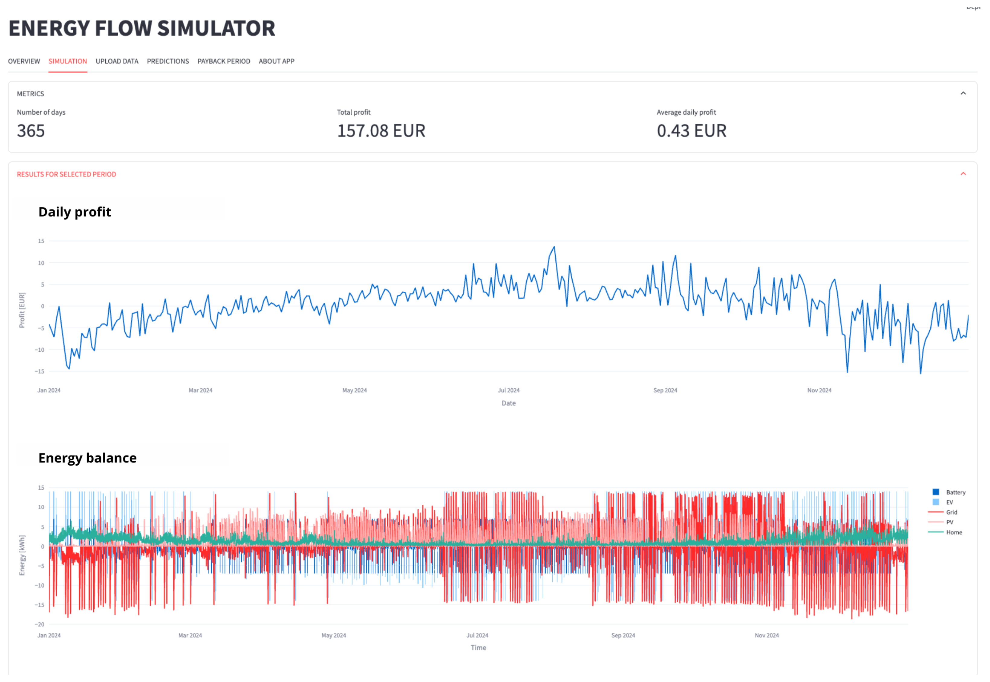
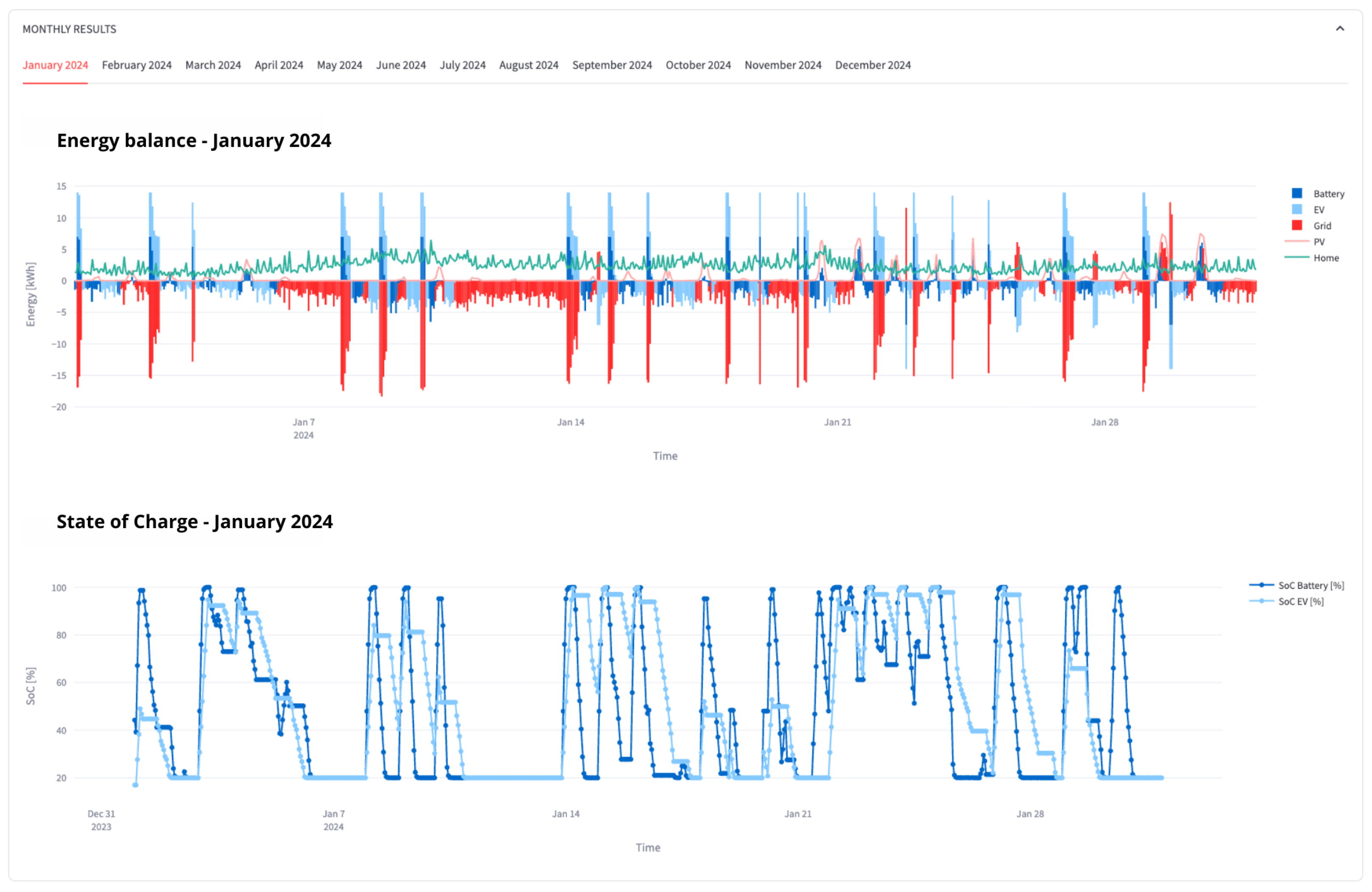
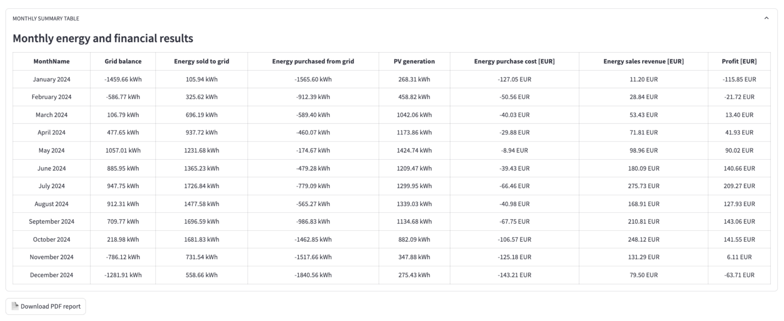
This chapter presents the results of the simulations carried out and examines their significance. The examination includes both the reference case, in which electricity is supplied solely from the grid (no EV), and a range of EV scenarios featuring different technical characteristics. Furthermore, configurations that include PV installations together with additional BESS are investigated.

The calculations aim to assess the influence of EV and storage system parameters, as well as their availability profiles, on annual electricity purchase costs, battery cycle counts, and energy utilization efficiency indicators. The results provide insights into the most cost-effective and efficient solutions for incorporating electromobility into prosumer energy systems.

5.1. Simulation Parameters

To obtain robust simulation results, it is essential to specify a set of parameters that affect the analytical results. These parameters cover the facility’s characteristic profiles of energy demand and production, as well as the technical characteristics of the EV and the auxiliary BESS. The use of real-world data provides a realistic representation of actual operating conditions and facilitates analysis of the extent to which specific system components affect electricity costs, battery cycle counts, and overall efficiency of energy utilization.

The key parameters to be specified are:

• Electricity costs, including variable electricity tariffs, grid distribution fees, fixed charges, and supplementary fees (e.g., VAT);
• The energy consumption profile of the building;
• The PV production profile;
• The EV availability profile and mBESS characteristics, including capacity, charging power, efficiency, and maximum DoD;
• BESS characteristics, including capacity, charging power, efficiency, and maximum DoD.

Simulation data were sourced from operating facilities to ensure realistic modeling conditions. To ensure reliability and diversity, the study utilizes an empirical dataset from a real single-family household in Poland, covering the entire year of 2024. The dataset provides a comprehensive and high-resolution view of all energy flows, including PV generation measured every 5 min, hourly measurements of energy imported from and exported to the grid, total household electricity demand, and hourly DAM prices from the TGE platform. This dataset captures seasonal variability and allows the EMS to be tested under different electricity tariffs and multiple EV models, ensuring that the simulations reflect real-world operational conditions and varying market scenarios. The statistical characteristics of the dataset, including energy consumption, PV generation and market prices [48] are summarized in

Table 3. Statistical characteristics of the dataset (hourly values).

Statistic	Consumption [kWh]	PV Generation [kWh]	DAM Price [EUR/kWh]
Mean	1.10	1.24	0.0975
Median	0.83	0.00	0.0931
Std. Dev.	0.94	2.14	0.0513
Min	0.00	0.00	−0.0842
Max	7.74	9.89	0.6436
5th Percentile	0.15	0.00	0.0163
25th Percentile	0.38	0.00	0.0756
75th Percentile	1.52	1.45	0.1140
95th Percentile	3.08	6.39	0.1768

.

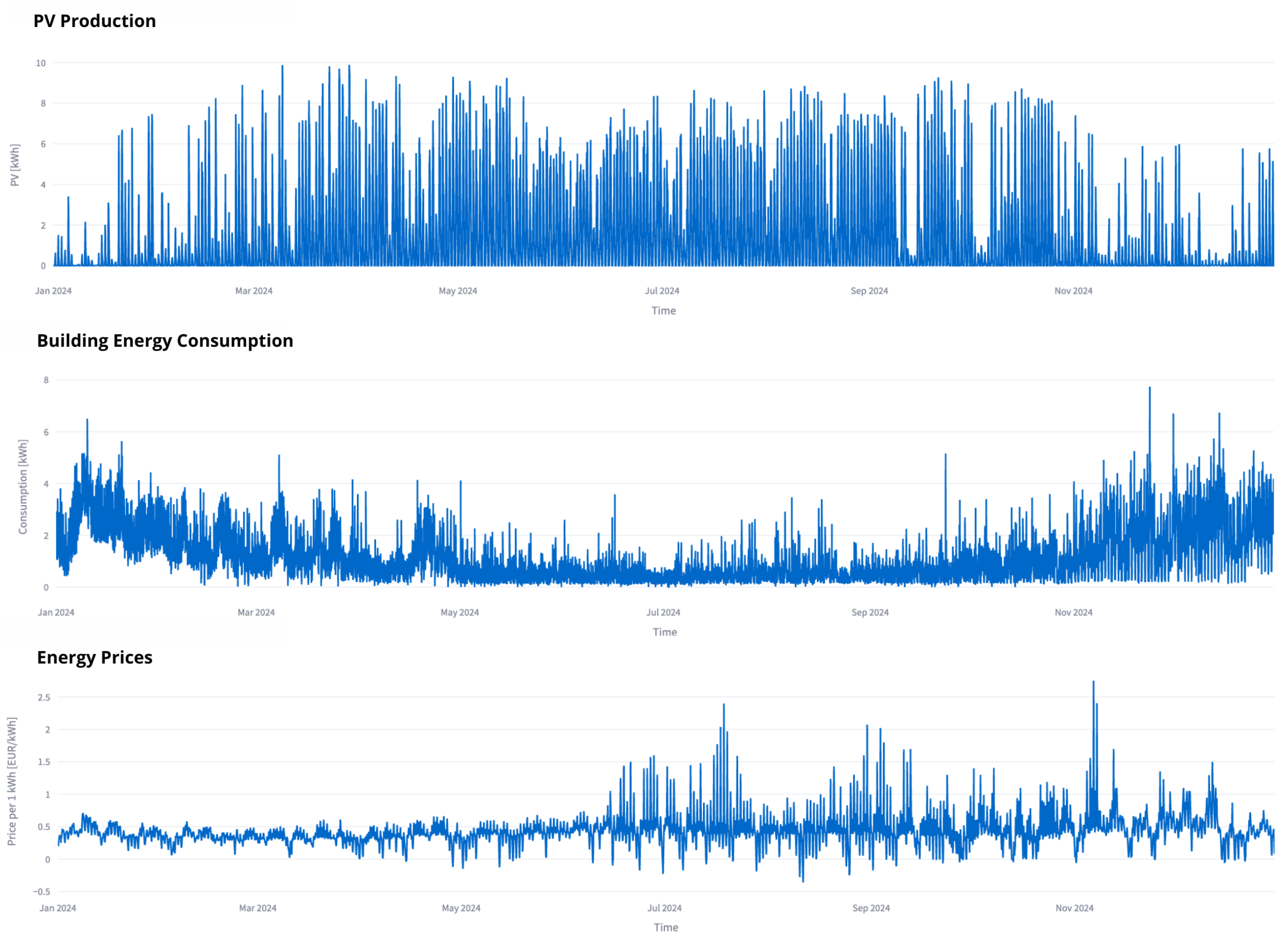
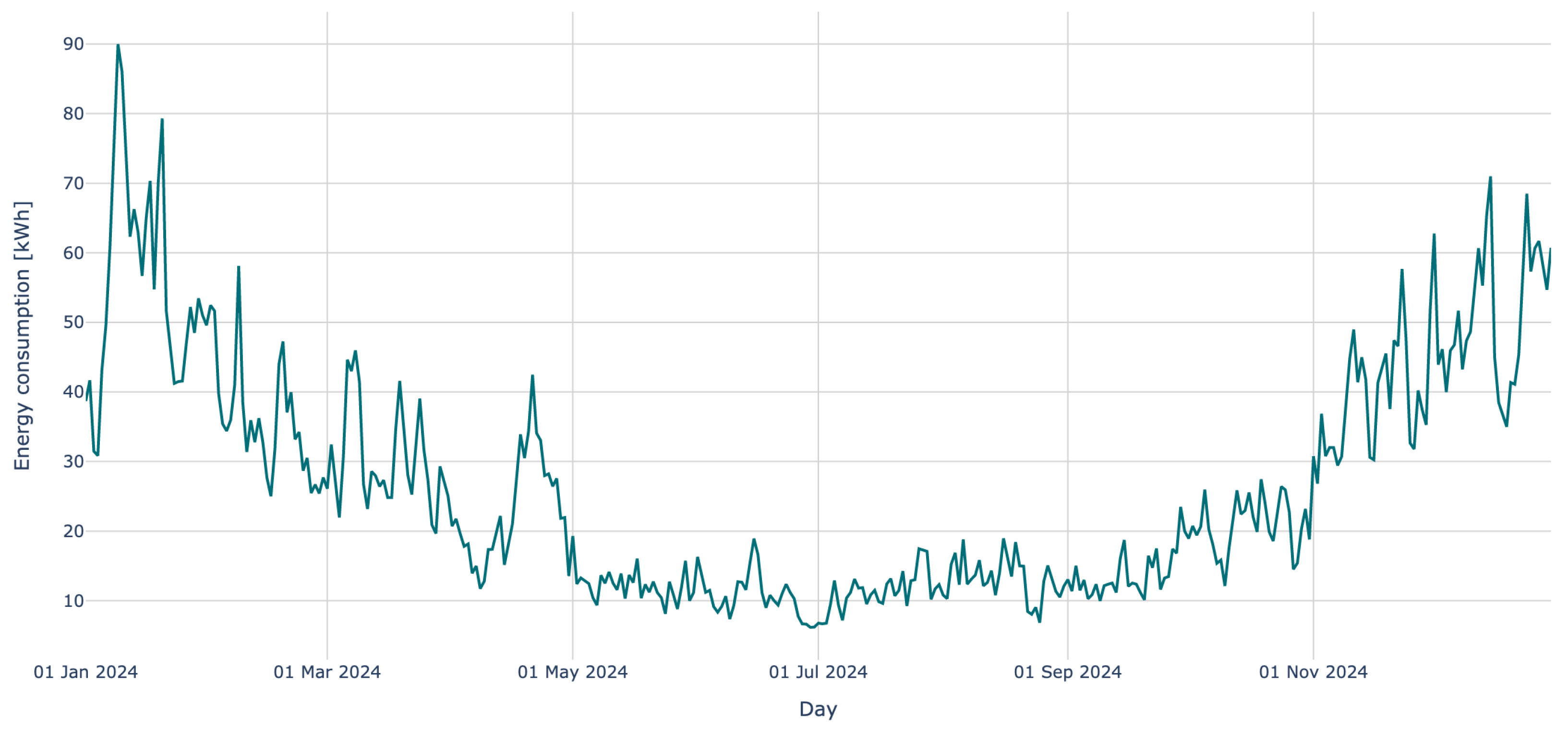
The energy consumption dataset pertains to a detached single-family dwelling with a usable floor area of 160 m², occupied by two adults and one child. Space heating and domestic hot water demand is met by a 16 kW heat pump. The corresponding daily energy consumption profile is presented in Figure 9.

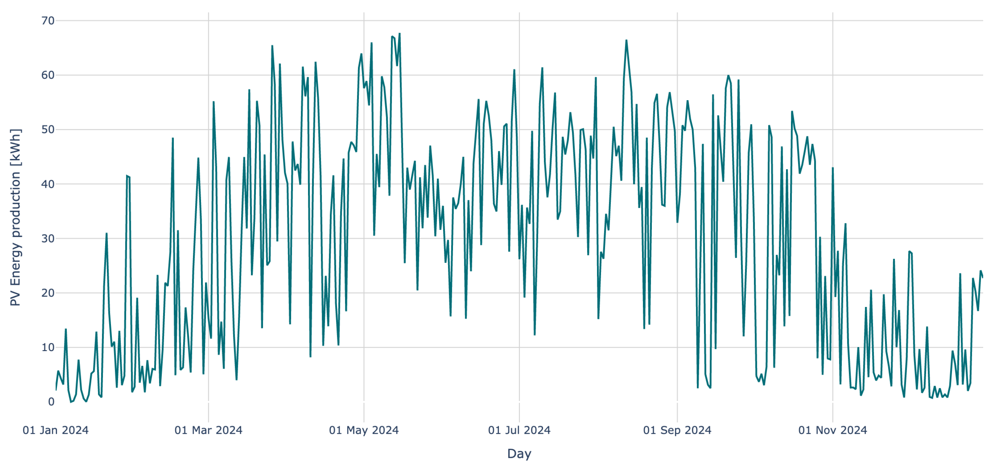
The simulation additionally incorporated the increasing penetration of micro-installations within the Polish power system. For this purpose, data from a 9.92 kWp ground-mounted PV system, facing south with a tilt angle of 35°, were employed. The daily electricity production of the system in 2024 is shown in Figure 10.

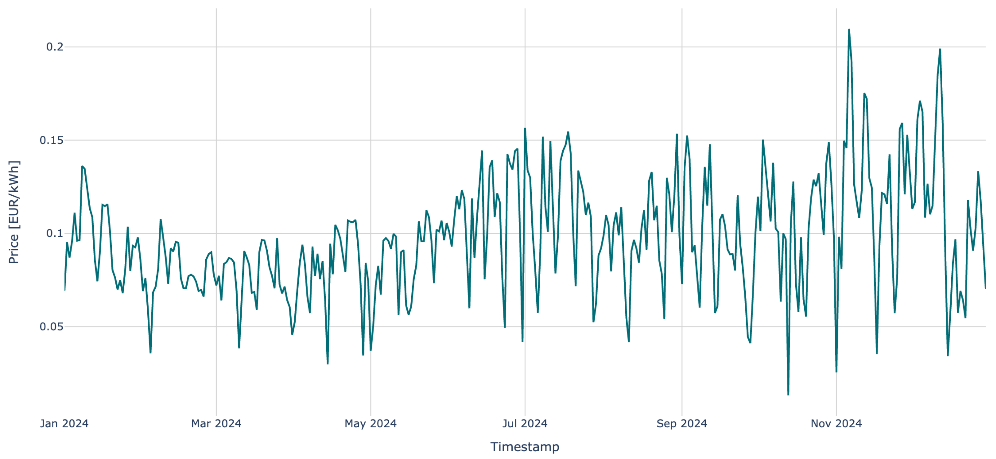
To accurately reflect the real market conditions, electricity prices from the TGE DAM were used. The average daily prices in 2024, based on Fixing I quotations, are shown in Figure 11.

The Polish power system is served by four principal distribution system operators (DSOs): PGE Distribution, Tauron Distribution, Enea Operator, and Energa-Operator. Their key tasks include ensuring a secure and continuous electricity supply to consumers, upgrading and maintaining the distribution grid, and implementing solutions that support the functioning and evolution of the energy markets.

Among these entities, Energa-Operator was one of the first companies in Poland to offer end users access to time-varying electricity prices. This was achieved through the introduction of the G11f tariff for household customers. The tariff allows consumers to react to price signals and shift their electricity use depending on the time of day, which can lower their energy expenditures and improve overall energy efficiency.

For reference, in 2024 the G11 tariff remained the most widely used in Poland. Under this tariff, the electricity rate is fixed and does not vary by time of day, day of the week, or month. Although this solution is straightforward and offers consumers a high degree of predictability, it provides no incentive to adjust or optimize the electricity consumption patterns.

In the same year, the Polish government implemented protective measures for household customers and introduced a maximum electricity price of 0.117 EUR/kWh. In the absence of these interventions, the market price would have surpassed 0.14 EUR/kWh [49].

In Poland, electricity purchase costs consist of both fixed and variable components. Variable costs are directly proportional to the volume of electricity consumed, while fixed costs are determined by the contracted capacity, the level of annual consumption, and the length of the billing period.

Table 4. Variable electricity costs for tariffs G11 and G11f [50].

Cost Component	G11 [EUR/kWh]	G11f [EUR/kWh]
Net energy price	0.117	DAM energy price
Variable distribution charge	0.080	0.012
RES fee	0.00082	0.00082
Cogeneration fee	0.00070	0.00070
Quality charge	0.00751	0.00751
Excise duty	0.00117	0.00117
Net total	0.207	0.0223 + DAM price
VAT rate	23%	23%

provides an overview of the variable electricity costs for the G11 and G11f tariff groups. The key distinction between these two tariff groups with respect to variable costs is a reduction in the distribution charge by more than 0.068 EUR/kWh for G11f, along with the incorporation of DAM prices.

Determining fixed charges first requires specification of the connection parameters and estimation of the annual electricity demand. The building under examination relies on a heat pump as its primary energy source; therefore, higher annual electricity consumption and peak demand are required. As a result, a three-phase connection is necessary, generating monthly fixed costs of 2.70 EUR under the G11 tariff and 12.76 EUR under the G11f tariff. If a single-phase connection were sufficient, these amounts would decrease to 1.80 EUR and 9.05 EUR, respectively [50]. Due to the substantial power demand, both the capacity and the transitional charges were set to their maximum values. A comprehensive overview of the fixed charges, assuming the examined building and a monthly settlement period, is provided in

Table 5. Fixed monthly electricity costs for tariffs G11 and G11f [50].

Cost Component	G11 [EUR]	G11f [EUR]
Fixed distribution charge (three-phase)	2.70	12.73
Capacity fee	3.75	3.75
Subscription fee	0.17	0.17
Transition fee	0.077	0.077
Fixed monthly total (three-phase)	6.70	16.75
VAT rate	23%	23%

.

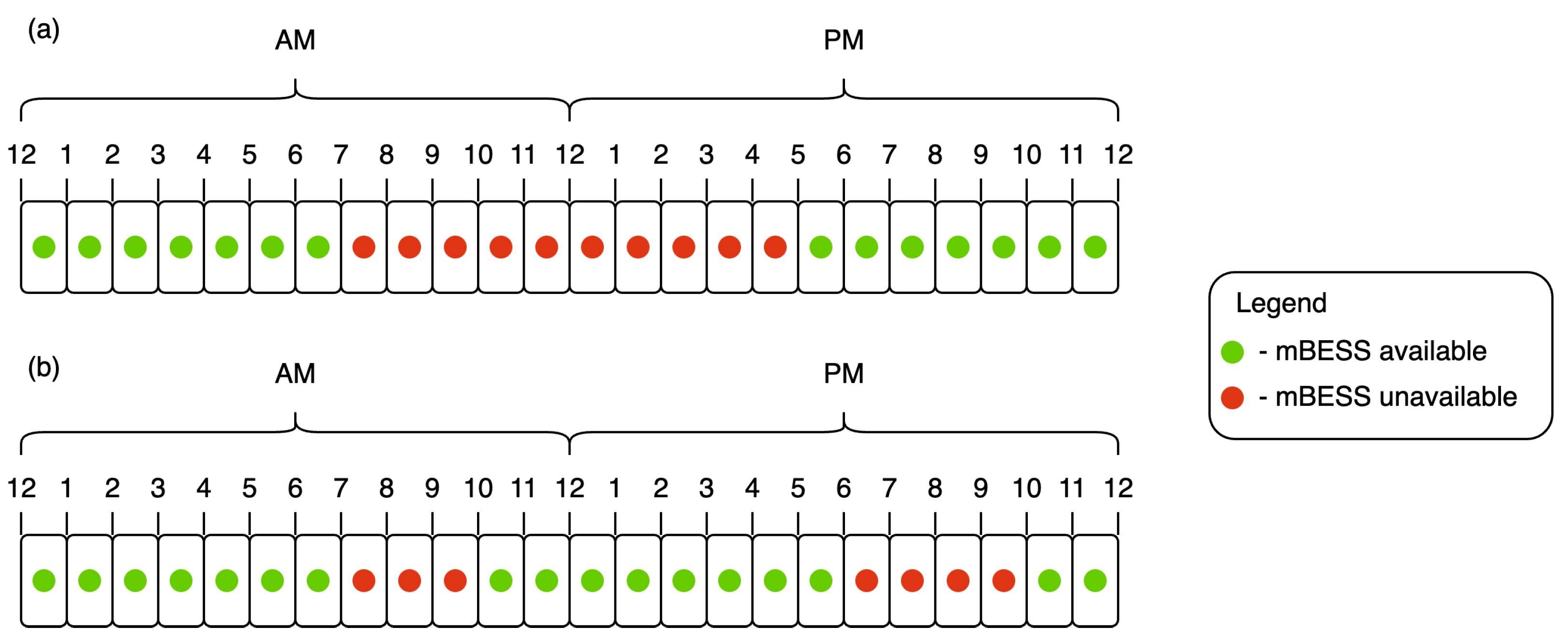
The operation of an EV as an mBESS is feasible only during the periods when it is connected to the power grid. To assess the impact of EV availability on energy yield, two distinct EV usage profiles were defined, as illustrated in Figure 12. The first profile corresponds to users with a standard work schedule from 8 a.m. to 4 p.m., during which the EV is away from home and thus unavailable from 7 a.m. to 5 p.m., totaling 10 h per day. The second profile represents a remote worker whose EV is unavailable in the morning, for example, due to school drop-offs, and again in the afternoon for activities such as shopping or gym visits. These profiles capture different patterns of EV availability and highlight that the primary function of the EV is transportation, while it simultaneously operates as an mBESS.

5.2. Simulation Results

In the initial stage of the simulations, the differences between fixed and variable costs were determined for the analyzed facility. The facility’s annual electricity consumption amounts to 9629.09 kWh. Energy procurement costs under the G11f tariff were evaluated using DAM prices from the TGE. The first simulation scenario did not include a BESS, an mBESS, or a PV system. In the second scenario, electricity generation from the PV installation was incorporated, along with the resulting revenues from energy sales and savings from self-consumption. Revenues from electricity exported to the grid were calculated using the hourly net-billing mechanism based on DAM prices. For PV installations, the user is not billed for the energy returned to the grid during hours with negative prices. The energy purchase costs are summarized in

Table 6. Annual electricity costs: G11 vs. G11f, with and without PV (EUR).

Type of Cost	G11 [EUR]	G11f [EUR]	G11 + PV [EUR]	G11f + PV [EUR]
Fixed costs	98.8	246.7	98.8	246.7
Variable costs	2456.3	1429.3	1273.9	525.8
Total costs	2555.1	1676.0	1372.7	772.5

.

In the G11f tariff group, fixed charges are higher than in the G11 tariff by approximately 150%, primarily due to the increased monthly fees associated with a three-phase connection.

In contrast, the variable component of the G11f tariff is roughly 42% lower than that of G11, resulting in significant reductions in annual electricity expenditure. For the G11 tariff, the total energy cost amounts to 2555.10 EUR, while for the G11f tariff it is 1676.00 EUR. Consequently, despite higher fixed charges, the reduced variable costs lead to a total annual savings of 879.10 EUR.

Integration of PV systems further enhances economic performance. Under both tariffs, the use of self-generated PV electricity leads to a substantial decrease in variable costs: a portion of the energy is consumed directly on-site, while any excess is exported to the grid. The most advantageous outcome is observed for the G11f tariff, where combining PV with hourly DAM pricing enables optimal exploitation of the lowest hourly rates. Consequently, the total annual costs in the G11f scenario with a PV system are more than three times lower than in the G11 tariff without a PV system.

In the following stages of the analysis, the influence of coefficients $\alpha$ and $\beta$ on costs was assessed as a function of the EV usage profile and EV type.

The simulation was carried out under the following assumptions:

• Battery efficiency was fixed at 80%.
• The maximum DoD was limited to 70%.
• Energy consumption associated with EV driving was excluded from the simulation to isolate the marginal economic performance of the EMS strategy and avoid results being skewed by highly variable individual mobility patterns.
• The initial state of charge of the mBESS was set to 10 kWh.
• The maximum charging and discharging power of the mBESS depends on the specific EV or charger.
• The mBESS capacity is determined by the particular EV model under analysis.

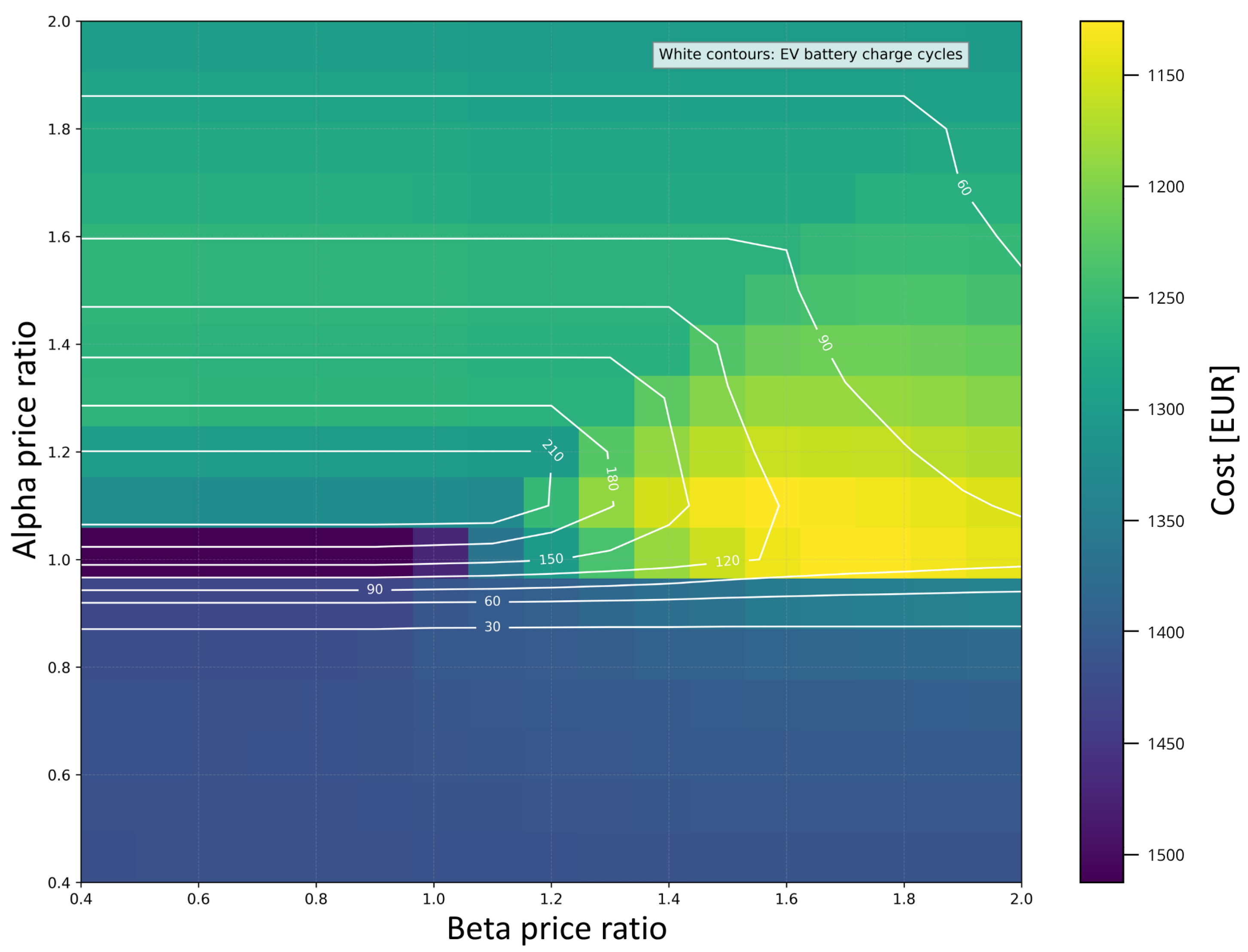
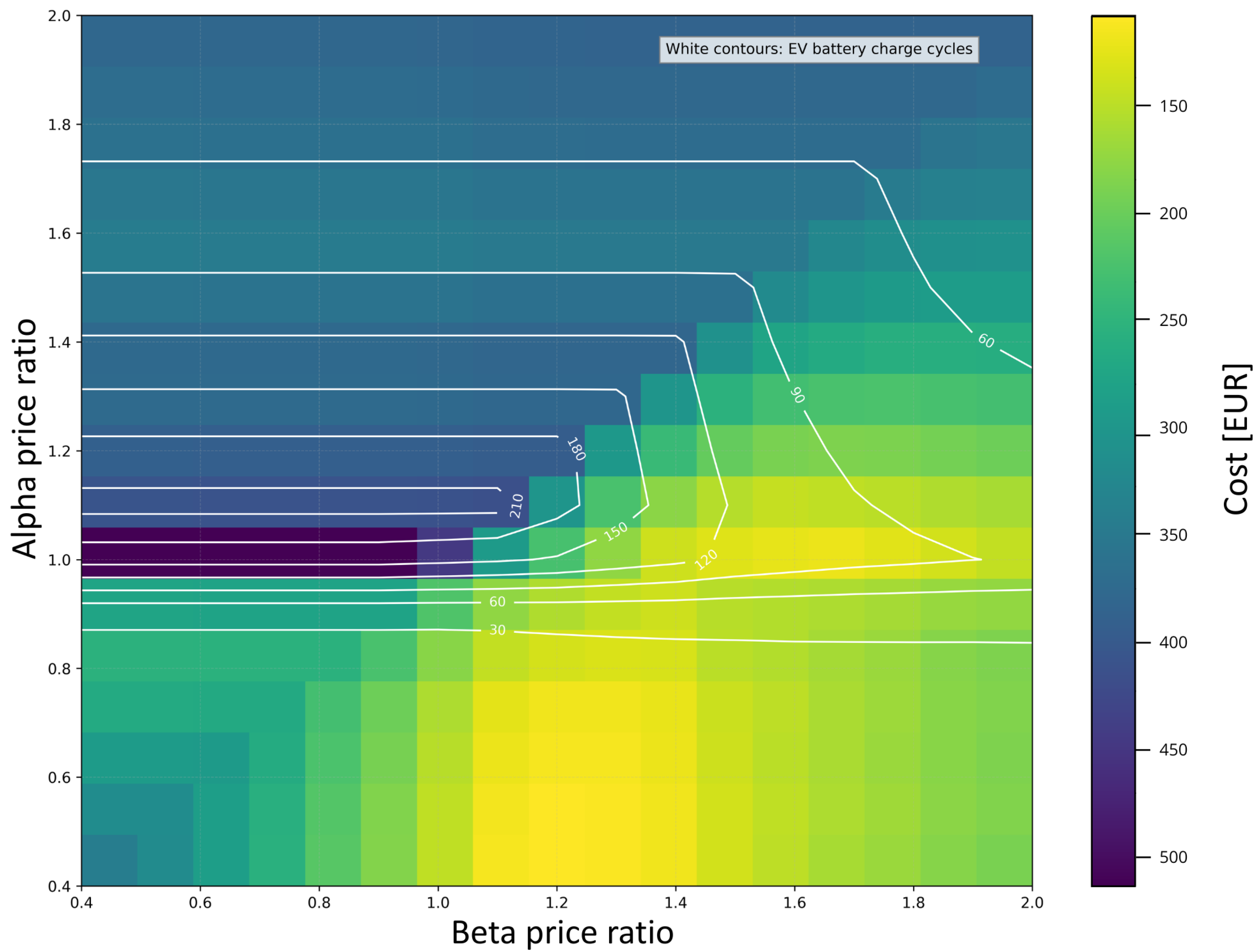
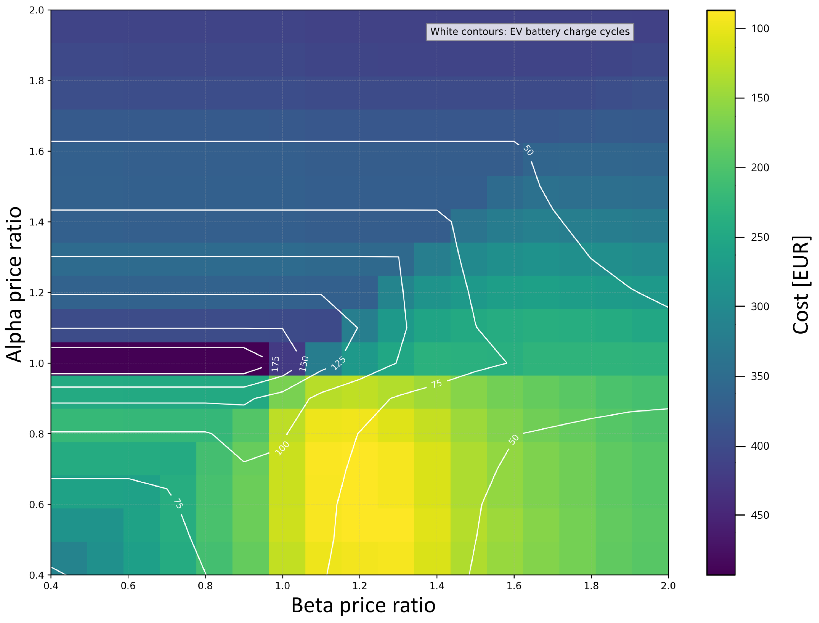
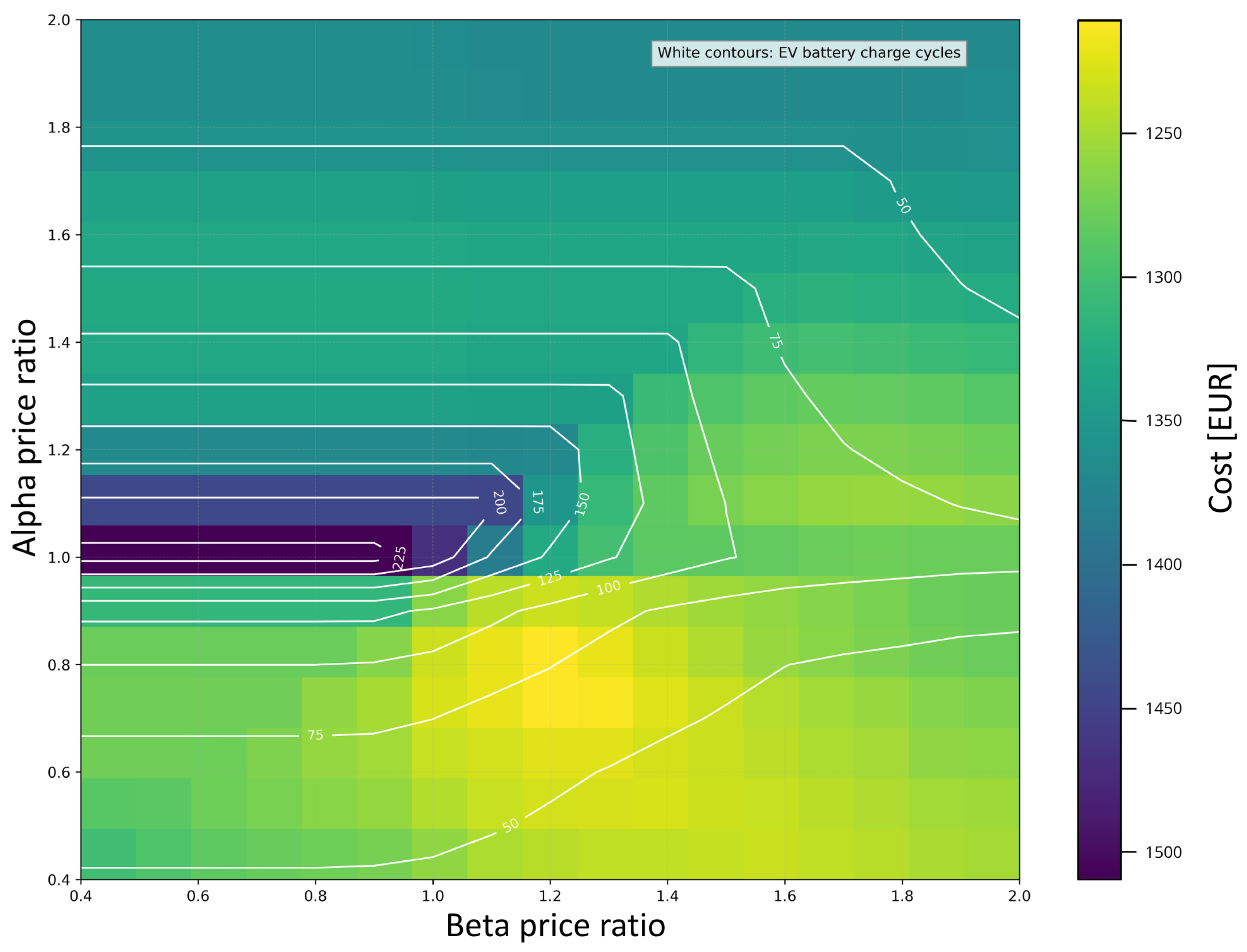
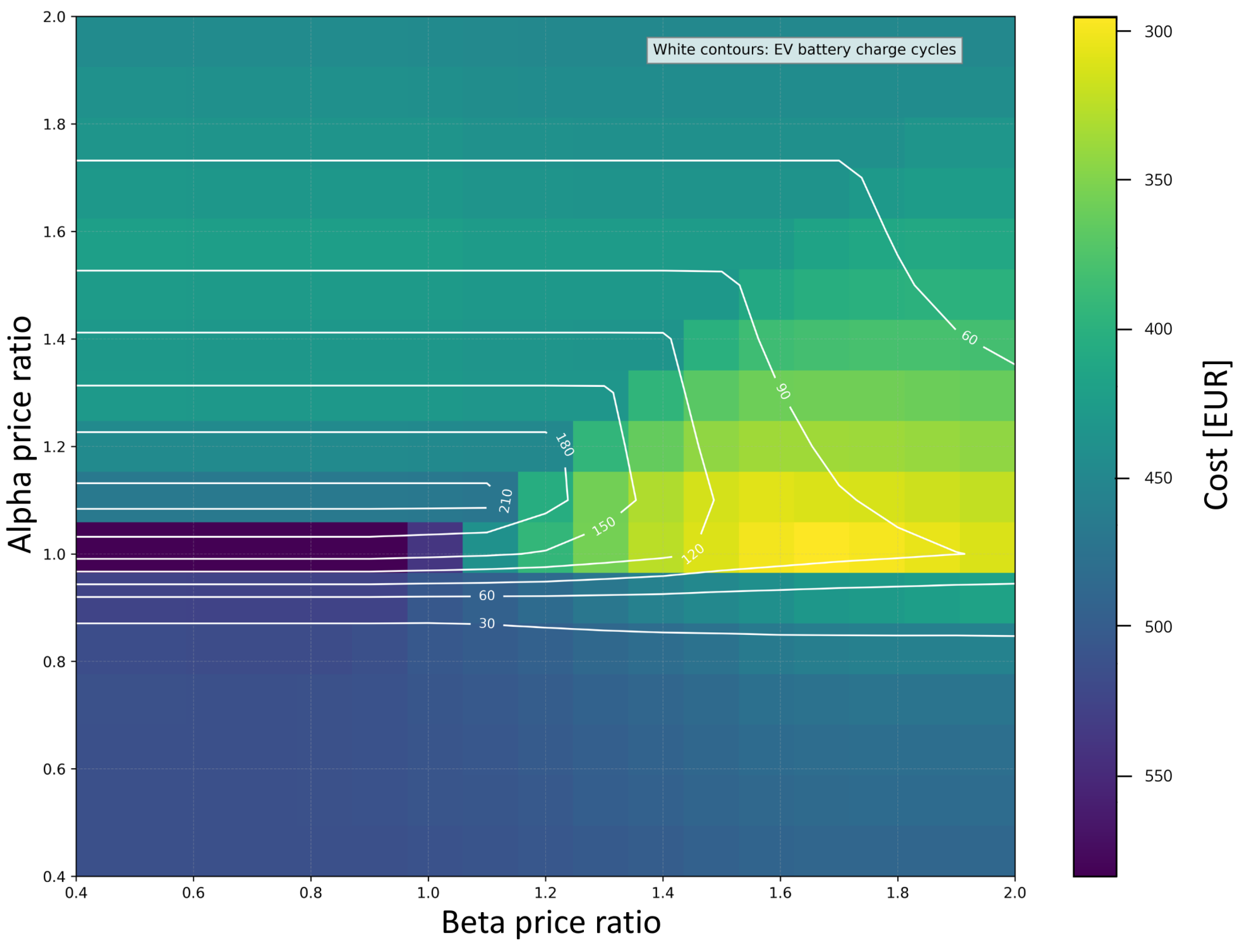
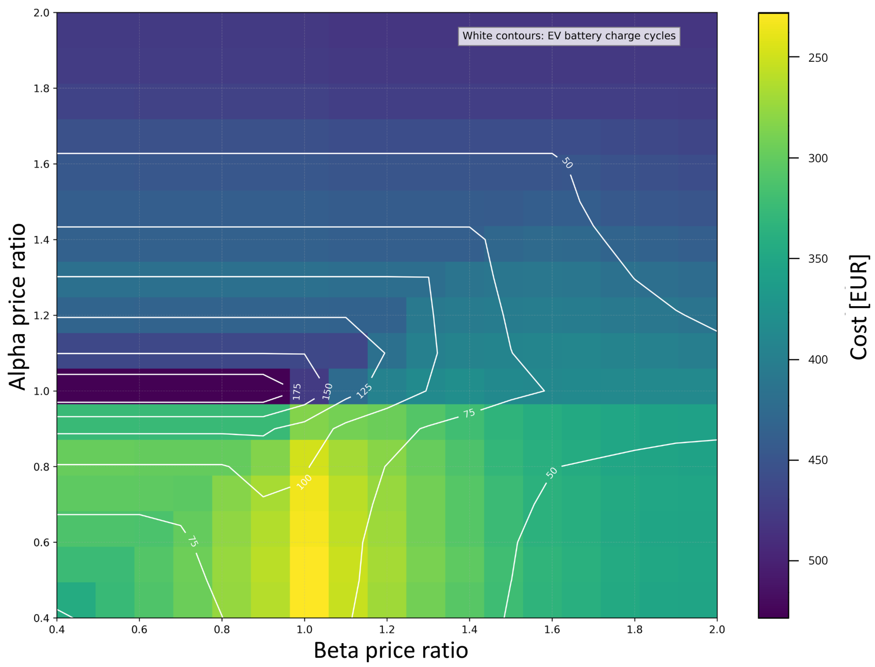
The initial set of simulations evaluated annual electricity purchase costs in two configurations: one including only an EV operating as an mBESS and another combining the mBESS with a PV installation. These simulations were performed for three EV models with different battery capacities and charging powers. For the Nissan Leaf e+, Figure 13, Figure 14, Figure 15 and Figure 16 present the annual variable energy purchase costs and the corresponding number of mBESS charging cycles for two EV availability profiles, both without and with a PV system. The results are shown as functions of the price coefficients $\alpha$ and $\beta$, which vary from 0.4 to 2.0 in steps of 0.1. The selected range was determined based on preliminary simulation analysis, which indicated that for values exceeding 2.0 the occurrence of energy selling events becomes negligible, whereas for values below 0.4 energy purchasing is infrequent, leading to limited utilization of the storage system. Therefore, the adopted range represents a practically relevant operating domain. In additional tests with increased resolution (step of 0.02), the location and extent of the most profitable $\alpha$–$\beta$ regions remained practically unchanged, confirming that the chosen step of 0.1 provides sufficient detail for capturing performance trends while maintaining computational efficiency. The figures also report the number of mBESS charging cycles.

For Profile 1 (without PV), shown in Figure 13, the most favorable outcomes are achieved for $\alpha$ values between 0.95 and 1.15 and $\beta$ values in the range of 1.5 to 1.9. In this region, the number of mBESS charging cycles ranges from 90 to 120, resulting in a minimum variable cost of 1140 EUR.

For Profile 2 (without PV), illustrated in Figure 14, the optimal parameter zone shifts toward lower $\alpha$ values (0.7–0.8) and $\beta$ values (1.1–1.3). Within this range, the number of charging cycles is reduced to 60–80, while the minimum variable cost amounts to 1210 EUR.

The subsequent simulations incorporated the PV system. For Profile 1 with a PV system (Figure 15), the heat map pattern remains largely unchanged compared to the non-PV scenario, with optimal results observed for $\alpha$ between 1.0 and 1.1 and $\beta$ between 1.5 and 1.9. The battery undergoes 90 to 120 cycles, and the minimum variable cost is reduced to 296 EUR.

A significant alteration in the heat map pattern occurs for Profile 2 with a PV system, as shown in Figure 16. In this configuration, the most advantageous results are achieved for $\alpha$ values between 0.4 and 0.8 and $\beta$ set to 1.0. Within this interval, the mBESS performs between 80 and 100 cycles, and the annual energy purchase cost reaches its lowest point at 224 EUR.

To evaluate the system’s robustness, the analysis examines the percentage deviations from the optimal annual cost caused by variations in the $\alpha$ and $\beta$ coefficients.

Table 7. Sensitivity analysis of annual cost increase due to individual and combined parameter selection errors ($\alpha$, $\beta$).

		Error ± 0.2				Error ± 0.4
EV Model	Availability Profile	$\mathit{\alpha }$	$\mathit{\beta }$	Combined		$\mathit{\alpha }$	$\mathit{\beta }$	Combined
Nissan Leaf e+	Profile 1	21.92%	2.66%	22.34%		23.46%	9.38%	23.81%
	Profile 2	1.94%	1.52%	4.48%		11.88%	4.12%	25.03%
	Profile 1 + PV	56.28%	5.12%	61.26%		62.95%	20.40%	68.42%
	Profile 2 + PV	1.34%	20.98%	22.32%		8.93%	37.05%	38.39%

summarizes these deviations for each scenario, considering both individual and combined parameter changes. This approach provides a quantitative measure of the objective function’s sensitivity to potential parameter selection errors. By highlighting the worst-case deviations within the specified ranges ($\pm 0.2$ and $\pm 0.4$), the analysis defines a clear economic safety margin for EMS operation.

The percentage deviations highlight that the algorithm’s robustness is strongly influenced by both the specific availability profile and the inclusion of renewable energy sources. Scenarios based on Availability Profile 1 exhibit a steeper cost increase, where even minor changes in the $\alpha$ coefficient result in noticeable departures from the optimum. For Profile 1 with a PV system, the combined deviation reaches 61.26% for a $\pm 0.2$ shift. This high percentage is mainly due to the low baseline cost (224 EUR), where small absolute differences translate into large relative changes. In contrast, configurations using Availability Profile 2 show greater stability, particularly regarding the price-sensitivity parameter. The data also indicate a non-linear accumulation of errors when both coefficients deviate by $\pm 0.4$, especially in PV systems. This pattern confirms that while the EMS can tolerate minor configuration errors, achieving maximum economic benefit in PV systems necessitates a more precise calibration of the $\alpha$ values.

The spatial distribution of the yields on the heat map as a function of the coefficients $\alpha$ and $\beta$ remains largely consistent across the different EV models, despite increases in charging power with battery capacity. In contrast, both energy procurement costs and the number of charging cycles exhibit notable variations.

Table 8. Comparison of annual EV performance including baseline (no EV).

EV Model	Capacity [kWh]	Power [kW]	Availability Profile	Cost [EUR]	Number of Cycles	$\mathit{\alpha }$	$\mathit{\beta }$	Savings [%]
No EV	–	–	Profile 1/2	1429	–	–	–	0.0
			Profile 1/2 + PV	525	–	–	–	0.0
Nissan Leaf e+	59	7	Profile 1	1140	110.4	1.0	1.7	20.2
			Profile 2	1210	62.9	0.7	1.2	15.3
			Profile 1 + PV	296	98.7	1.0	1.7	43.6
			Profile 2 + PV	224	90.6	0.5	1.0	57.3
Volkswagen ID.7	82	10	Profile 1	1058	100.8	1.0	1.7	26.0
			Profile 2	1137	62.5	0.7	1.2	20.4
			Profile 1 + PV	238	89.3	1.0	1.7	54.7
			Profile 2 + PV	157	78.8	0.4	1.0	70.1
Polestar	111	11	Profile 1	1020	83.0	1.0	1.7	28.6
			Profile 2	1084	53.3	0.7	1.2	24.1
			Profile 1 + PV	215	80.7	1.0	1.6	59.0
			Profile 2 + PV	109	64.4	0.4	1.0	79.2

summarizes the simulation results for the Nissan Leaf e+, VW ID.7, and Polestar for various mBESS operating profiles and PV system configurations. The table reports the optimal values of $\alpha$ and $\beta$ that minimize energy procurement costs, along with the corresponding number of charging cycles and the percentage savings relative to the baseline scenario.

Comparative analysis with the reference case demonstrates a substantial savings potential. Depending on the chosen coefficients and EV model, an mBESS can reduce annual electricity costs by several hundred to over a thousand EUR. The most significant reductions occur for EVs with larger battery capacities and higher charging power as they offer enhanced flexibility in energy shifting and can more effectively capture volatile price signals. Furthermore, the results are sensitive to the EV availability profile: Profile 1 is more cost-effective in scenarios without PV due to afternoon price peaks, whereas Profile 2 excels when integrated with a PV system as it allows for better buffering of peak solar generation.

In the next set of simulations, an additional BESS was incorporated with the following parameters:

• Capacity: 20 kWh;
• Charging power: 5 kW;
• Maximum DoD: 80%;
• Efficiency: 80%.

The analyses were carried out for a Nissan Leaf e+, considering two charging profiles with and without a PV installation.

The impact of this additional storage on energy costs and the yield pattern is illustrated in Figure 17 for Profile 1 with a PV system. The integration of a BESS substantially alters the heat-map characteristics, expanding the range of $\alpha$ and $\beta$ coefficients that yield significant savings. Specifically, two clearly differentiated high-potential regions emerge:

• Region 1: $\alpha \approx 1.0$ with $\beta$ between 1.5 and 1.8;
• Region 2: $\alpha$ between 0.4 and 0.7 combined with $\beta$ between 1.1 and 1.4.

In these zones, the joint operation of mBESSs and BESSs achieves the maximum reduction in procurement costs. At the optimal operating point, the annual energy cost drops to approximately 112 EUR. This represents an additional saving of roughly 184 EUR compared to the scenario with only the EV and PV (where costs totaled 296 EUR), demonstrating the BESS’s role in stabilizing the system and further maximizing the utilization of available energy.

For Profile 2 with a PV system (Figure 18), the integration of a BESS further enhances system efficiency. The optimal results are concentrated at $\alpha$ between 0.4 and 0.8 and $\beta$ between 1.1 and 1.3, where the annual energy cost drops to approximately 27 EUR. This represents an additional saving of 197 EUR compared to the mBESS+PV scenario (224 EUR), with the battery performing 60 to 85 charging cycles.

A summary of the annual energy purchase costs, accounting for the addition of the BESS, is provided in

Table 9. Comparison of annual performance of Nissan Leaf e+ with additional BESS.

EV Model	Capacity [kWh]	Power [kW]	Availability Profile	Cost	mBESS Cycles	BESS Cycles	$\mathit{\alpha }$	$\mathit{\beta }$	Savings [%]
Nissan Leaf e+	59	7	Profile 1	946.00	106.0	212.4	1.1	1.7	33.8
			Profile 2	1005.00	66.3	146.7	0.8	1.3	29.7
			Profile 1 + PV	112.00	9.0	211.2	0.4	1.2	78.7
			Profile 2 + PV	27.00	69.0	126.6	0.5	1.2	94.9

. The findings confirm that integrating stationary storage leads to a radical reduction in expenditures across all scenarios, with total annual savings exceeding 468 EUR relative to the baseline (no EV, no BESS). The most significant economic benefit is observed in Profile 2 with a PV system, where costs are reduced to a near-negligible level of 27 EUR. This underscores the critical role of the BESS as a stabilizing and complementary component; it effectively “fills the gaps” in the mBESS’s availability. By buffering surplus solar energy during periods when the EV is away from the facility, the BESS maximizes self-consumption and prevents the export of energy at less favorable prices. Furthermore, the presence of stationary storage broadens the range of optimal price coefficients $\alpha$ and $\beta$, making the control strategy more robust and less sensitive to precise parameter tuning. This synergy between mobile and stationary storage proves to be the most effective approach for achieving near-complete energy independence in residential buildings.

Ultimately, the integration of a stationary BESS not only drastically reduces annual energy expenditures but also expands the range of optimal price-factor combinations, confirming its essential role as a stabilizing and high-performance complement to mBESSs.

5.3. Economic Analysis

The economic feasibility of integrating EV into home energy ecosystems is based on the strategic assumption that the EV is a pre-existing primary asset. Since the vehicle’s primary purpose is transportation, its battery capacity-acting as an mBESS—is treated as an underutilized resource. This analysis evaluates the incremental costs required to transform a standard EV into an active grid participant. The necessary infrastructure includes a bidirectional DC charger providing a minimum power of 11 kW and a dedicated EMS. For this study, a cost-effective implementation is assumed, utilizing, e.g., Raspberry Pi as the central controller to execute optimization algorithms. To evaluate the economic viability of these configurations, two key financial indicators are employed: the Simple Payback Period (PBP), representing the time in years required for annual savings to recover the initial capital expenditure (CAPEX), and the Return on Investment (ROI), which quantifies annual profitability as a percentage of the total investment.

The investment scenarios are defined as:

• mBESS Integration: Includes a bidirectional charger (2500 EUR) and an RPI-based EMS (100 EUR), totaling a CAPEX of 2600 EUR. The comparative analysis for various EV models is presented in

  Table 10. ROI analysis for EV models (mBESSs).

  EV Model	Availability Profile	Cost [EUR]	Profit [EUR]	PBP [Years]	ROI [%]
  Nissan Leaf e+	Profile 1	1140	289	9.0	11.1
  	Profile 2	1210	219	11.9	8.4
  	Profile 1 + PV	296	229	11.4	8.8
  	Profile 2 + PV	224	301	8.6	11.6
  VW ID.7	Profile 1	1058	371	7.0	14.3
  	Profile 2	1137	292	8.9	11.2
  	Profile 1 + PV	238	287	9.1	11.0
  	Profile 2 + PV	157	368	7.1	14.2
  Polestar	Profile 1	1020	409	6.4	15.7
  	Profile 2	1084	345	7.5	13.3
  	Profile 1 + PV	215	310	8.4	11.9
  	Profile 2 + PV	109	416	6.3	16.0

  .
• mBESS + BESS Integration: Includes the mBESS infrastructure and a stationary BESS (8000 EUR), totaling a CAPEX of 10,600 EUR. The results for this configuration are shown in

  Table 11. ROI analysis for Nissan Leaf e+ with additional BESS.

  Configuration	Availability Profile	Cost [EUR]	Profit [EUR]	PBP [Years]	ROI [%]
  Nissan Leaf e+ + BESS	Profile 1	946	483	21.9	4.6
  	Profile 2	1005	424	25.0	4.0
  	Profile 1 + PV	112	413	25.7	3.9
  	Profile 2 + PV	27	498	21.3	4.7

  .

To assess the financial impact, profitability is benchmarked against two baseline scenarios: a standard grid-tied household with an annual energy cost of 1429 EUR (without PV) and a prosumer household with a baseline cost of 525 EUR (with a PV system).

The mBESS Integration scenario, which focuses on the purchase of a bidirectional charger and an EMS (totaling 2600 EUR), shows a relatively fast payback period. For modern EVs like the Polestar or VW ID.7, the investment can break even in just 6 to 7 years, providing an attractive ROI of 14–16%. In contrast, the mBESS + BESS configuration reveals a much harsher financial reality. The high cost of BESSs—estimated at 8000 EUR for a 20 kWh unit—triples the initial investment to 10,600 EUR. While this setup maximizes energy autonomy and achieves record-high annual savings, the disproportionately high CAPEX pushes the payback period to over 21 years. Realistically, such an investment exceeds the typical warranty period of most residential battery systems, making it a strategic choice for energy independence rather than a rapid financial gain.

Modern EVs predominantly utilize lithium-ion battery technology. The round-trip efficiency (RTE) of lithium-ion cells typically ranges from 78% to 98%, depending on the specific chemistry and design [51,52,53]. However, when considering the entire energy management chain, including power converters, the battery management system, and thermal regulation, the overall system-level RTE is approximately 80% [54], representing a conservative median value for residential energy storage applications [55]. This efficiency is not constant and depends on operational factors such as C-rate, ambient temperature, and the applied SoC range. Techno-economic analyses of BESSs indicate that a variation in cycle efficiency of ±5 percentage points typically results in changes in annual cost indicators in the range of 0.5–4.5% [56]. Since only a fraction of the total energy exchanged within the system passes through the storage unit, these efficiency variations translate into an overall impact of approximately ±2–5% on the annual energy cost balance. Consequently, although such deviations introduce a degree of uncertainty, they do not affect the qualitative conclusions regarding the economic viability of the analyzed configurations.

Importantly, the profitability of these systems is not significantly affected by battery degradation costs. Recent studies indicate that the additional annual degradation associated with V2G operation is relatively low, typically ranging from 0.35% to 1.4% [57]. This resilience is primarily due to the use of low C-rates—by limiting charging power to 7–11 kW, the system operates at a small fraction of the battery capacity, reducing thermal and mechanical stress compared to high-power DC fast charging. Moreover, an EMS can mitigate calendar aging—the natural degradation occurring during idle periods—by optimizing the SoC and avoiding prolonged exposure to high voltage levels [12].

To quantify this impact over the long term, the standard cycle life of modern EV batteries must be considered, which typically ranges between 1500 and 3000 cycles before reaching the 80% State of Health (SoH) threshold. In the highest-profit scenario for the Polestar (Profile 2 + PV), which yields 416 EUR in annual savings, the system executes approximately 65 full equivalent cycles per year. Based on a conservative average life of 2000 cycles, this operational intensity would result in a 20% SoH loss over approximately 30.7 years, far exceeding the typical operational lifespan of the vehicle. Even in the most demanding case, the Nissan Leaf e+, with roughly 110 annual cycles, the 20% degradation threshold would not be reached for approximately 18.2 years. These figures demonstrate that the additional wear caused by V2G is well within the design limits of modern battery technology, ensuring that the economic gains are not offset by premature asset depreciation.

6. Conclusions

The simulation results indicate that the deployment of EVs as mBESSs is an effective approach to reducing electricity procurement costs. The achievement of near-optimal results critically depends on the selection of price coefficients $\alpha$ and $\beta$, which influence both economic savings and the frequency and depth of ESS charge–discharge cycles.

The economic and operational performance of the system is determined by several technical and operational parameters:

• Power output and generation profile of the PV installation;
• Capacity and charging power of mobile and stationary ESSs;
• EV availability profiles;
• Permissible depth-of-discharge limits and energy conversion efficiency;
• Tariff structure and distribution-related fees.

Distribution costs have a pronounced impact on the economic performance of the system. Low distribution charges allow increased numbers of charging and discharging cycles to enhance profitability, while high distribution costs favor energy procurement during low-price periods and electricity sales during peak-price periods, thereby reducing the significance of cycle frequency.

Integration of EMSs with both mBESSs and BESSs enables substantial reductions in electricity procurement costs. When combined with a PV installation, total annual energy expenditures can be reduced to a marginal level. Moreover, systems characterized by high storage capacity and charging power can effectively exploit market price volatility by purchasing electricity during periods of low or negative prices and subsequently reselling it to the grid.

Furthermore, the inclusion of BESSs enhances overall system flexibility and broadens the range of price parameters, for which near-optimal performance can be achieved, ensuring stable economic benefits under varying operating conditions. The selection of system parameters must be tailored to the specific layout of the installation and the characteristics of the facility, which can be achieved using dedicated simulation software capable of evaluating different configurations involving PV, ESSs, and EVs. Such tools allow users to define parameters including PV capacity, storage size, and power rating in order to maximize cost savings or revenue.

In general, the proposed methodology supports both economic and technical planning and optimization of energy systems according to predefined criteria, such as electricity expenditure and the number of storage charging cycles.

Despite the promising results, several practical limitations must be considered. The widespread implementation of V2G and V2H technologies is still constrained by the limited availability of bidirectional chargers, regulatory barriers, and the lack of standardized market mechanisms enabling full participation of residential users. Moreover, current grid infrastructure and operational standards may restrict the extent to which distributed energy resources, such as EVs and BESSs, can actively participate in energy markets. Issues such as grid stability, connection capacity, and communication protocols remain critical challenges. Therefore, while the proposed EMS demonstrates significant economic potential under dynamic pricing conditions, its real-world deployment depends on further technological development, regulatory support, and market integration. Importantly, the proposed approach demonstrates that meaningful economic benefits can be achieved using a transparent and computationally efficient control strategy, without relying on complex optimization or forecasting models, which makes it particularly suitable for real-world residential applications under current technological and regulatory constraints.

It should also be noted that the performance of the EMS strongly depends on the selection of the control coefficients $\alpha$ and $\beta$, which define the thresholds for energy purchasing and selling relative to the moving average price. In particular, when $\alpha$ is very low and $\beta$ is high, the system purchases energy frequently but sells it only rarely, which can limit the effective utilization of the storage system. Conversely, when both $\alpha$ and $\beta$ are high, the system tends to purchase energy more readily but may sell it only during pronounced price peaks, resulting in frequent charging but less frequent discharging events. These observations highlight that different parameter combinations correspond to distinct market strategies, ranging from conservative to more aggressive participation. Importantly, no single set of parameters can be considered universally optimal. For example, in strategies focused on exploiting large price spreads, lower $\alpha$ and higher $\beta$ values may be more beneficial, while more balanced strategies may rely on higher $\alpha$ values to ensure more regular charging. Therefore, the selection of $\alpha$ and $\beta$ should be aligned with the intended market strategy and the desired trade-off between risk, system utilization, and economic performance.

Finally, it is important to emphasize that the presented results were obtained under the assumption that traction energy consumption is excluded in order to isolate the effects of the EMS. Therefore, the reported cost reductions should be interpreted as indicative of the relative performance of the models rather than directly achievable savings in real-world EV operation.

Future Works

Further research will also investigate to what extent the current rule-based strategy can be complemented or replaced by optimization-based control schemes that explicitly use these forecasts, and how different EMS approaches perform under varying market conditions and tariff structures. An inherent limitation of the current study is that the performance of the price-driven, rule-based EMS is not explicitly benchmarked against a “perfect foresight” strategy that minimizes annual electricity costs with full knowledge of future prices and operating conditions. In principle, such a benchmark could be implemented, for example, by always charging the storage during the cheapest hours and discharging during the most expensive hours, subject to the same technical constraints on power, capacity, SoC and EV availability. While the present work systematically explores the performance of the $\alpha$ and $\beta$ coefficients and identifies wide regions in which near-minimal annual costs are achieved, it does not quantify the exact percentage of the theoretical maximum savings that these coefficients deliver. Providing a formal comparison with a perfect-foresight or optimization-based benchmark is therefore left for future research, where the proposed rule-based strategy can be evaluated in terms of its relative economic efficiency. Although we do not explicitly implement a perfect-foresight benchmark in this study, previous comparisons between rule-based EMSs and optimization-based or MPC controllers for residential PV-battery systems indicate that well-designed rule-based strategies typically capture on the order of 80–95% of the theoretically achievable cost savings, with remaining gaps in the range of approximately 5–15% depending on system sizing and tariff structures.

An additional research direction concerns the integration of additional components of the energy system. Hybrid configurations, including thermal storage units and heat pumps operating in coordination with the EMS, can be considered to improve overall system efficiency and enable more advanced energy management across multiple energy carriers. Moreover research should focus on compliance with emerging standards such as ISO 15118, to ensure practical applicability and scalability of the proposed approach.

Another important aspect is the evaluation of different EV charging technologies and power levels, together with the assessment of long-term battery degradation effects. Future research will also aim to incorporate variable charge/discharge efficiency models that depend on current, SoC, and temperature, to more accurately capture the impact of operational conditions on energy losses and battery performance. This will complement aging models and enable a more comprehensive analysis of the trade-off between operational cost reduction and storage lifetime.

Finally, the software framework may be extended to support larger-scale installations or multi-building systems, enabling the analysis of shared energy resources and coordinated control strategies. This would increase the applicability of the proposed approach and strengthen its value as a practical tool for the design and optimization of advanced EMSs.