Optimal Design Arrangement for Suppressing Supercritical CO₂ Heat Transfer Deterioration by Deep Learning and Genetic Algorithm

Abstract

Supercritical carbon dioxide (CO₂) is a promising working fluid for advanced power cycles. However, under high heat flux and low mass flux, its heat transfer performance can deteriorate severely, posing significant risks to system safety and efficiency. Inserting obstacles into flow channels is an effective way to suppress such heat transfer deterioration (HTD). In this study, the body-centered cubic (BCC) lattice structure is taken as an example to investigate the effects of the number and arrangement of BCC units on the flow and heat transfer of supercritical CO₂ using numerical simulation, deep learning, and genetic algorithms. The results show that placing a BCC lattice structure upstream of the HTD temperature peak effectively improves local heat transfer, and the deterioration zone is shifted downstream. For a fixed number of BCC units, different spatial arrangements have little impact on pressure drop and only a limited effect on heat transfer enhancement. However, their influence on the suppression of HTD is very significant. Based on the analysis of the optimal arrangement, an approximate optimal method is obtained, in which BCC structures are inserted sequentially at locations 0.5 to 2 tube diameters (D) upstream of each wall temperature peak. A simplified yet effective design strategy is also proposed: the first BCC structure is placed 0.5 to 2 D upstream of the smooth tube’s temperature peak, and the remaining BCC units are then distributed uniformly along the subsequent flow length. In this way, effective suppression of heat transfer deterioration is achieved.

1. Introduction

Supercritical carbon dioxide (CO₂), characterized by its high density, low viscosity, and excellent heat transfer capabilities, has emerged as an ideal working fluid for thermodynamic power cycles [1,2]. The compact architecture of supercritical CO₂ Brayton cycles further enhances their application potential in fields with space constraints and high power demands [3,4], such as aviation and marine propulsion, as well as in engine regenerative cooling, thermal protection, and thermal management systems [5,6]. However, compared to subcritical fluids, the flow and heat transfer characteristics of supercritical CO₂ are considerably more complex, particularly near the pseudo-critical point where drastic variations in thermophysical properties lead to unexpected heat transfer performance. Under conditions of low mass flux and high wall heat flux, the induced phenomenon of heat transfer deterioration (HTD) [7,8] results in a precipitous drop in the local heat transfer coefficient and a rapid rise in the inner wall temperature, ultimately compromising both the performance and operational safety of heat exchange equipment.

A consensus holds that buoyancy [9] critically affects heat transfer deterioration in supercritical CO₂ channel flows. Jackson’s work [10] on upward vertical flow explains that changes in fluid properties and gravity generate buoyancy forces which modify the radial distribution of shear stress, thereby weakening turbulent heat diffusion and thus causing HTD, which is especially pronounced under low mass flux and high heat flux conditions. Furthermore, many studies [11,12,13] indicate that drastic variations in thermophysical properties are an important cause of abnormal heat transfer phenomena, such as heat transfer enhancement and heat transfer deterioration, with the most severe property changes occurring particularly in the vicinity of the pseudocritical region. To suppress HTD in tubular flows [14], researchers have proposed various strategies, including modifying tube geometry, incorporating internal obstacle structures, and implementing more refined flow control through induced vortex systems. Ackerman [15] experimentally studied the heat transfer and friction characteristics of supercritical water flowing through uniformly heated, internally ribbed tubes with diameters of 10 mm and 25 mm. The conclusion was that internally ribbed tubes promote the energy and mass exchange within the tube for supercritical fluids, thus effectively suppressing HTD, albeit with a flow friction approximately 25% higher than that of smooth tubes. Furthermore, variable-diameter channels and corrugated tubes were selected for suppressing supercritical fluid HTD: Lau [16] suggested the use of converging–diverging (variable-diameter) tubes and corrugated tubes to suppress HTD in supercritical water. Building upon this, Yang [17] considered the coupling of nanofluids with variable-diameter channels to further enhance the heat transfer capacity of supercritical fluids, numerically investigating the combined effect of corrugated tubes and nano-Fe₃O₄ on HTD suppression in supercritical water.

Additionally, some scholars have investigated obstacle structures in channels for HTD suppression [18]. Bae [19] experimentally investigated the influence of inserted helical wire structures on the flow and heat transfer characteristics of supercritical CO₂ in a vertical circular tube. The results showed that the helical wire structure increased the convective heat transfer coefficient by nearly a factor of two, indicating its effectiveness in enhancing heat transfer performance and suppressing HTD. Wang et al. [20] employed a complex wire matrix structure inserted into supercritical nitrogen for heat transfer enhancement. The intricate structure effectively promoted cross-sectional temperature mixing, thereby suppressing HTD. Eter et al. [21,22] experimentally studied the effects of single, side-attached obstacles of different shapes (such as circular bluff bodies) on the flow and heat transfer characteristics of supercritical CO₂ in smooth tubes. The experimental results indicated that a single, side-attached obstacle object could effectively suppress HTD at its location. However, as the fluid moved away from the obstacle structure, a temperature peak re-emerged downstream. When multiple obstacle structures were arranged within the channel, periodic temperature fluctuations were observed along the flow direction. Eze [23] numerically explored the use of internal annular-rib-type vortex generators for enhancing and suppressing HTD in supercritical water, noting that the rib size influenced HTD suppression and that an optimal size existed. Hu [24] investigated HTD suppression in supercritical water by adding star-shaped spacers within the channel. The research results showed significant heat transfer enhancement near the spacers, followed by distinct HTD further downstream. Cao [25] attempted to suppress HTD in supercritical CO₂ by installing a Helmholtz self-excited oscillation cavity upstream of the channel inlet. The cavity generated pulsating impinging flow, which enhanced fluid disturbance and turbulent intensity within the tube, thereby partially suppressing the buoyancy-induced HTD. Inspired by the compact structure and low flow resistance of lattice structures [26], Yang and Shi [27,28] conducted some studies on the influence of lattice structures on suppressing HTD. Considering the trade-off between the heat transfer enhancement and additional pressure drop, among various lattice structures, the Body-Centered Cubic (BCC) lattice, due to its simple and symmetric geometry, effectively suppressed HTD while incurring the smallest flow friction, yielding the highest thermal efficiency index.

However, a single obstacle structure is often insufficient to completely suppress HTD distributed along the flow direction [21,22], necessitating analysis of the arrangement of such flow obstacles. Therefore, this paper takes the BCC lattice structure as a case study and first discusses how factors such as the quantity and arrangement of lattice structures within a channel influence the heat transfer characteristics, friction characteristics, and HTD suppression performance for supercritical CO₂. Subsequently, a deep learning method combined with a genetic algorithm is employed for the optimal design of the spatial arrangement of lattice structures within the channel. Based on input sensitivity analysis, a fast and simplified optimization design method for arranging flow obstacles is proposed for engineering applications.

2. Methodology

2.1. Physical Model

To investigate the impact of the BCC (Body-Centered Cubic) lattice arrangement on heat transfer deterioration (HTD) in supercritical CO₂ flows, a baseline case exhibiting pronounced HTD within a smooth circular tube was first established. The operating parameters were defined as follows: inlet temperature T_in = 295 K, operating pressure P = 7.8 MPa, inlet mass flux G = 320 kg/(m²·s), constant wall heat flux q = 60 kW/m², tube inner diameter D = 6 mm, BCC ligament diameter d = 0.1 D = 0.6 mm, and total heated length L = 40 D = 240 mm. A RANS simulation based on the numerical methodology detailed in Section 2.2 was conducted for this configuration. The resulting wall temperature distribution presented in Figure 1 confirms a distinct HTD characterized by a sharp wall temperature peak at an axial location of z = 6.33 D (38 mm). This case serves as the baseline for all subsequent comparative analyses.

To enable a quantitative study and optimization of spatial arrangements, a formalized representation method for BCC lattice arrangements is proposed: under the constraints of preventing incomplete lattice units and physical interference between adjacent structures, the maximum allowable number of BCC units within the channel length L is denoted as n. The minimum center-to-center distance between two BCC units, occurring when their ligaments are in contact, is defined as l_min. For any specific design incorporating m BCC units (where 0 ≤ m ≤ n), the spatial array is uniquely described by a tensor [x₁, x₂, …, x_n]. Here, x₁ represents the distance from the channel inlet to the center of the first BCC unit, subject to the constraint x₁ ≥ 0.5 l_min. For i > 1, x_i denotes the distance between the centers of the (i − 1)-th and i-th BCC units, requiring x_i ≥ l_min for 1 < i ≤ m. For non-existent BCC units (i > m), the value is set to zero (x_i = 0). Furthermore, to ensure the final BCC unit is entirely contained within the channel, the summation must satisfy ∑x_i ≤ L − 0.5 l_min. A schematic exemplifying this quantification method is provided in Figure 2 as [x₁ = 23, x₂ = 93, x₃ = 28, 0, …, 0].

2.2. Numerical Method

The numerical simulations for the current study were performed with the commercial software ANSYS CFX 18.1. The steady-state Navier–Stokes equations were discretized and solved using the finite volume method. For turbulence closure, the shear stress transport (SST) k-ω model [29] was employed, as it is well-suited for flows with substantial flow separation. Gravity is retained in the present model, as it plays a critical role in the heat transfer deterioration of supercritical CO₂ flows. In contrast, viscous dissipation is neglected, which is justified by the low Mach number (well below 0.3) characterizing the flow. The governing equations are presented as follows:

Continuity equation:

$${\displaystyle \frac{\partial \left(\rho u_i\right)}{\partial x_i}}=0,$$

(1)

Momentum equation:

$${\displaystyle \frac{\partial \left(\rho u_i{u}_j\right)}{\partial x_j}}=-{\displaystyle \frac{p}{x_i}}+{\displaystyle \frac{\partial }{\partial x_j}}\left[\mu {\displaystyle \frac{\partial \left(u_i\right)}{\partial x_j}}-\rho \overline{u_i^{\prime }{u}_j^{\prime }}\right]+\rho g,$$

(2)

Energy equation:

$${\displaystyle \frac{\partial }{\partial x_i}}\left(\rho T\right)+{\displaystyle \frac{\partial }{\partial x_i}}\left(\rho u_{i}T\right)={\displaystyle \frac{\partial }{\partial x_i}}\left[{\displaystyle \frac{\lambda }{c_p}}{\displaystyle \frac{\partial T}{\partial x_i}}\right],$$

(3)

Equation of the turbulent kinetic energy (TKE):

$${\displaystyle \frac{\partial (\rho k{u}_i)}{\partial x_i}}={\displaystyle \frac{\partial }{\partial x_j}}\left[\left(\mu +{\displaystyle \frac{{\mu }_t}{{\sigma }_k}}\right){\displaystyle \frac{\partial k}{\partial x_j}}\right]+G_k-Y_k,$$

(4)

Turbulent dissipation rate equation:

$${\displaystyle \frac{\partial (\rho \omega u_i)}{\partial x_i}}={\displaystyle \frac{\partial }{\partial x_j}}\left[\left(\mu +{\displaystyle \frac{{\mu }_t}{{\sigma }_{\omega }}}\right){\displaystyle \frac{\partial \omega }{\partial x_j}}\right]+G_{\omega }-Y_{\omega }+D_{\omega },$$

(5)

The formula for k and ω includes multiple components, such as the production term indicated by G, the dissipation of turbulence denoted as Y, and the cross-diffusion term labeled D_ω. Turbulence closure was achieved via the shear stress transport (SST) k-ω model, a choice particularly effective in capturing extensive flow separation. Among various RANS models, this approach has been demonstrated to yield reliable predictions [17], and its model constants can be configured as suggested in [29]. In view of the sharp variations in the thermophysical properties of supercritical CO₂ near the pseudo-critical point, the TASC flow RGP format file generated from NIST REFPROP 9.11 was employed to specify these properties as functions of temperature and pressure. As for the meshing scheme, tetrahedral elements were used to discretize the computational domain. Moreover, 20 prism layers with a height ratio of 1.05 were constructed to maintain the dimensionless wall distance y⁺ below 1.0. A more comprehensive description for the numerical method can be found in refs. [27,28].

2.3. Validation of the Numerical Study

To further validate the applicability of the numerical method adopted in this study, numerical simulations were performed based on the experimental data of supercritical CO₂ heat transfer characteristics in vertical tubes reported by Eter [21] and Zhu [30], as shown in Figure 3 and Figure 4, respectively. Eter’s experiment represented a typical vertical upward flow condition with slight heat transfer deterioration (HTD). The test was conducted in a smooth circular tube with a wall heat flux of 15.9 kW/m², an inlet mass flux of 308 kg/(m²·s), and an outlet pressure of 7.75 MPa. In Zhu’s experiment, significant HTD was observed under a high-pressure condition far from the critical point, with a wall heat flux of 351.22 kW/m², an inlet mass flux of 1001.5 kg/(m²·s), and an outlet pressure of 15.565 MPa. The validation results indicate that the present numerical predictions agree well with the experimental data in regions without HTD under vertical upward flow conditions. Although certain discrepancies exist in predicting the magnitude of the temperature peak, the overall relative error remains within 4.5%. Due to inherent limitations of the current RANS method in handling heat transfer problems involving supercritical fluids, some inaccuracies are to be expected. Nevertheless, considering the computational cost and given that qualitative reliability has been verified, the method is still considered acceptable for analytical purposes in many studies. Therefore, the computational approach employed in this study could be considered reliable for capturing the flow and heat transfer characteristics of supercritical CO₂.

2.4. Deep Learning Method

A deep neural network was employed to develop a fast-prediction surrogate model for the heat transfer behavior of varying BCC array configurations. The model’s development involved defining the BCC arrangement and streamwise position as inputs; processing these through multiple hidden layers; and predicting the local temperature as the output. The specific network configuration is 8 (input)-60-60-60-60-1 (output), which is depicted in Figure 5, while the associated hyperparameters are defined in

Table 1. The model parameter settings for deep learning neural network.

No.	Corresponding Parameter	Option or Value
1	Activation function for hidden layer	LeakyReLU
2	Activation function for output layer	ReLU
3	Negative slope of LeakyReLU (α1)	0.01
4	Learning rate (α) in Adam	1 × 10−5
5	Hyperparameter β1 in Adam	0.9
6	Hyperparameter β2 in Adam	0.999
7	Small value (ε) in Adam	1 × 10−8

. The hyperparameters were determined through established practices and preliminary testing: LeakyReLU is used in hidden layers to mitigate the vanishing gradient issue, while ReLU in the output layer ensures non-negative predictions of ΔT*. The references on the Adam algorithm [31] provide rigorous discussion and justification for hyperparameter selection.

$$\mathrm{LeakyReLU}(z)=\max (0,z)+{\alpha }_1\min (0,z)=\left\{\begin{array}{c}z,\mathrm{when} z\ge 0\\ {\alpha }_{1}z,\mathrm{when} z<0\end{array}\right.,$$

(6)

$$\mathrm{ReLU}(z)=\max (0,z)=\left\{\begin{array}{c}z,\mathrm{when} z\ge 0\\ 0,\mathrm{when} z<0\end{array}\right.,$$

(7)

3. Results and Discussion

3.1. The Influence of BCC Lattice Spatial Arrangement on the Heat Transfer Performance of Supercritical CO₂

3.1.1. BCC Lattice Arrangement

Prior literature [21,22] suggest that a single obstacle structure is often insufficient to fully suppress HTD. To elucidate the localized effect, several random placements of a single BCC unit within the baseline channel were simulated. The results, categorized based on the BCC position relative to the inherent HTD peak location (z = 38 mm), are summarized in Figure 6. When the single BCC was positioned upstream of the temperature peak (Figure 6a), it effectively enhanced local heat transfer, reducing the wall temperature at its location. However, this intervention primarily resulted in a downstream shift of the HTD peak. Conversely, placing the BCC downstream of the peak (Figure 6b) had negligible mitigative effect on the upstream HTD phenomenon. While it induced local heat transfer enhancement in its immediate vicinity, a subsequent temperature rise and recurrent HTD were observed further downstream. This demonstrates that to influence the HTD process effectively, the first BCC structure must be situated upstream of the temperature peak. Moreover, the pressure drop distribution for different spatial arrangements of a single BCC lattice structure within a circular channel is listed in

Table 2. Pressure drop distribution of a single BCC lattice under various spatial arrangements.

Location of the BCC Lattice (mm)	Pressure Drop (Pa)
7	1851.57
20	1853.89
27	1851.11
38	1850.18
68	1847.41
86	1850.96
114	1849.98
122	1848.48
147	1849.07
168	1851.63
200	1850.27
220	1853.15

. Overall, it can be observed that the variation in pressure drop across different arrangement cases is minimal. By calculating the average pressure drop and evaluating the deviation for each case, the overall maximum variation is found to be approximately 0.35%. This result indicates that, for a single BCC lattice, its spatial position has a negligible impact on the overall pressure drop. Consequently, in subsequent analyses, it can be reasonably approximated that the spatial arrangement of a single BCC lattice does not affect the pressure drop. Therefore, when specifically evaluating the influence of the BCC lattice’s position, only the variation in heat transfer characteristics needs to be considered.

However, it should be acknowledged that the conclusion regarding the independence of pressure drop on spatial arrangement is drawn from the specific geometry and flow conditions examined in this study. The observed minimal variation in pressure drop (approximately 0.35%) may not universally hold for all geometries, Reynolds numbers, or obstacle configurations. For instance, in channels with significantly different aspect ratios, at substantially higher Reynolds numbers, or with obstacle shapes that induce stronger flow separation, the spatial arrangement may exert a more pronounced influence on pressure drop. Therefore, this finding should be interpreted as valid within the investigated parameter range, and caution is advised when extrapolating to markedly different conditions.

3.1.2. Thermal Performance of Uniform Multi-BCC Arrays Arrangement

This section further investigates the impact of uniformly arranged multiple BCC lattice structures on flow and heat transfer. Four configurations with 3, 5, 7, and 9 uniformly distributed BCC lattice structures inside the channel were investigated. These uniform arrangements can be quantitatively represented as: [60, 60, 60, 0, …, 0], [40, 40, 40, 40, 40, 0, …, 0], [30, 30, 30, 30, 30, 30, 30, 0, …, 0], and [24, 24, 24, 24, 24, 24, 24, 24, 24, 0, …, 0], respectively. Figure 7 presents the wall temperature distributions under different numbers of uniformly arranged BCC lattice structures, with the black curve indicating the wall temperature distribution in a smooth circular tube. Overall, the heat transfer characteristics within the channels exhibit periodic variations with changes in the number of BCC lattice structures. The case with 3 BCC lattice structures does not significantly suppress heat transfer deterioration (HTD), as the number of structures is small and they are all positioned downstream of the peak HTD temperature location. In contrast, in the case with 9 BCC lattice structures, the first structure is located upstream of the peak HTD temperature, and the subsequent structures are densely arranged. This configuration confines the overall temperature within a narrow fluctuation range. It can thus be concluded that if a sufficient number of BCC lattice structures are allowed, a uniformly arranged design can effectively suppress HTD.

The overall thermo-hydraulic performance is further assessed through the overall averaged Nusselt number (Nu_ave), friction factor (f), and thermal efficiency index (η = (Nu_ave/Nu₀)/(f/f₀)^1/3), as shown in Figure 8. As expected, both Nu_ave and f increase monotonically with the number of BCC lattices. Crucially, the efficiency factor η remains greater than 1.0 for all configurations, confirming that the benefit of heat transfer enhancement outweighs the penalty associated with increased flow friction, justifying the use of BCC arrays for performance promotion.

3.1.3. Thermal Performance of Non-Uniform Multi-BCC Arrays Arrangement

Based on the previous analysis, BCC lattice structures can be arranged as densely as possible within the overall system’s pressure drop allowance to achieve comprehensive suppression of heat transfer deterioration. Given that practical designs often operate under pressure drop limitations, optimizing the arrangement of a limited number of BCC units becomes essential. Since the configuration with 9 BCC lattice structures exhibits no local high-temperature zones and only minor temperature fluctuations, this section will focus on investigating the effects of non-uniform arrangements with 3, 5, and 7 BCC lattice structures within the channel on flow and heat transfer characteristics, aiming to explore optimization strategies for their layout. Through random sampling, 20 distinct arrangement cases were determined for each number (3, 5, and 7), and corresponding numerical simulations were conducted to obtain their flow and heat transfer performance. To quantitatively assess HTD suppression, the dimensionless temperature difference criterion proposed by Xie et al. [32] was employed:

$$\Delta T^{\ast }=\Delta T/\Delta T_{\mathrm{ref}}>1.0,$$

(8)

$$\Delta T_{\mathrm{ref}}=1.15\times \Delta T_{\mathrm{ave}},$$

(9)

$$\Delta T_{\mathrm{ave}}={\displaystyle \frac{{\displaystyle \int \Delta T\mathrm{d}x}}{x}}\approx {\displaystyle \frac{{\displaystyle {\sum }_n\Delta T}}{n}},$$

(10)

where ΔT represents the difference between the local wall temperature and the bulk temperature; ΔT_ref denotes the reference temperature difference, defined as 1.15 times the average temperature difference of the entire channel; ΔT_ave is the average temperature difference of the entire channel; and ΔT* is the local dimensionless temperature difference. A location is considered to be in a state of heat transfer deterioration when ΔT* exceeds 1.0. Therefore, evaluating whether ΔT*_max > 1.0 determines whether heat transfer deterioration occurs under the current conditions.

Table 3. Flow and heat transfer characteristics for different spatial arrangements of 3 BCC lattice structures within the channel.

No.	x1	x2	x3	Nuave	ΔT*max	ΔP
0	60	60	60	87.29	1.27	1919.18
1	133	44	41	85.24	1.45	1921.71
2	64	25	17	80.37	1.30	1914.49
3	106	90	12	84.73	1.44	1916.65
4	118	24	9	82.33	1.46	1913.97
5	35	39	35	98.63	0.84	1922.45
6	91	38	19	82.31	1.43	1917.04
7	23	43	52	92.65	0.98	1924.91
8	77	47	55	88.46	1.38	1922.09
9	13	107	48	88.63	1.35	1920.43
10	23	93	28	83.32	1.29	1919.64
11	50	59	48	84.70	1.18	1920.46
12	30	152	32	83.23	1.46	1918.49
13	83	55	18	89.16	1.40	1918.1
14	95	22	63	87.81	1.44	1919.17
15	29	107	92	81.45	1.35	1923.13
16	15	110	51	89.13	1.37	1922.29
17	27	17	20	86.43	1.43	1919.84
18	34	36	31	88.19	1.31	1924.12
19	10	119	38	88.22	1.40	1919.07
20	44	117	16	80.84	1.41	1914.73

,

Table 4. Flow and heat transfer characteristics for different spatial arrangements of 5 BCC lattice structures within the channel.

No.	x1	x2	x3	x4	x5	Nuave	ΔT*max	ΔP
0	40	40	40	40	40	116.94	0.83	1996.71
1	28	42	41	13	19	116.50	1.14	1990.89
2	49	47	70	36	17	109.34	1.08	1989.66
3	61	34	18	15	12	104.42	1.33	1980.87
4	27	45	23	52	69	115.01	0.70	1992.82
5	42	23	41	13	64	114.90	0.88	1988.02
6	98	70	26	18	14	104.65	1.44	1992.77
7	32	100	19	20	17	109.69	1.34	1989
8	40	29	39	63	16	115.16	0.82	1992.24
9	8	85	60	47	18	109.85	1.16	1989.24
10	70	53	19	12	17	111.07	1.35	1983.5
11	58	14	61	70	12	103.91	1.23	1983.72
12	34	14	48	19	26	114.99	1.20	1989.26
13	19	32	68	34	19	118.94	0.79	1989.78
14	55	61	15	27	25	113.74	1.20	1988.19
15	14	25	38	37	32	118.03	1.17	1995.05
16	11	67	30	33	39	118.43	0.79	1993.57
17	26	91	14	11	44	112.22	1.23	1986.21
18	52	76	56	27	10	102.92	1.15	1986.9
19	88	17	21	14	13	104.45	1.42	1985.08
20	104	27	13	13	21	110.30	1.45	1981.52

and

Table 5. Flow and heat transfer characteristics for different spatial arrangements of 7 BCC lattice structures within the channel.

No.	x1	x2	x3	x4	x5	x6	x7	Nuave	ΔT*max	ΔP
0	30	30	30	30	30	30	30	146.92	0.59	2065.45
1	8	46	51	37	11	60	18	140.67	0.58	2071.85
2	36	42	19	19	25	51	14	143.97	0.69	2057.34
3	42	38	11	65	17	43	9	133.96	0.89	2056.22
4	37	21	11	16	20	43	39	141.08	0.72	2055.14
5	33	36	56	27	11	31	39	138.35	0.64	2068.88
6	66	20	34	11	27	44	14	134.56	1.32	2055.69
7	34	26	52	49	47	15	11	135.64	0.65	2072.52
8	24	27	26	33	15	31	11	144.67	0.81	2053.99
9	22	49	50	31	16	38	23	140.59	0.58	2071.8
10	31	32	18	67	30	41	9	134.07	0.68	2064.04
11	35	24	38	17	28	44	28	143.55	0.65	2067.42
12	66	33	15	49	18	17	11	134.75	1.32	2056.02
13	41	45	51	53	15	11	9	133.52	0.86	2051.97
14	45	42	19	25	23	18	57	136.84	0.98	2062.06
15	7	64	59	21	12	12	38	138.76	0.72	2054.36
16	53	41	61	14	21	20	19	130.92	1.16	2060.16
17	48	14	50	60	20	14	13	132.06	1.03	2054.58
18	12	47	64	70	12	17	12	130.17	0.76	2070.08
19	43	16	60	44	45	13	11	129.80	0.90	2064.99
20	60	16	32	36	13	48	17	134.49	1.26	2060.73

present the computational results for the randomly sampled arrangements of 3, 5, and 7 BCC lattice structures, respectively. The quantitative representation follows the method described in Section 2.1. Entries where x_i = 0 are omitted in the tables, showing only values where x_i > 0. Each table lists the average Nusselt number (Nu_ave), pressure drop (ΔP), and maximum dimensionless temperature difference (ΔT*_max) for all cases. The first row in each table corresponds to the uniformly arranged configuration, followed by the 20 randomly generated arrangements.

The variation in pressure drop across each table leads to a conclusion similar to that for a single BCC lattice: the spatial arrangement has a minor impact on the overall pressure drop. For configurations with 3, 5, and 7 BCC units, the maximum relative variations in ΔP are only 0.57%, 0.72%, and 1.00%, respectively. Therefore, for a fixed number of BCC lattices, the influence of pressure drop can be neglected during optimization design, allowing the focus to remain solely on optimizing the heat transfer performance. Since the analysis of ΔP is equivalent to that of the friction factor (f), further consideration of f is unnecessary. Consequently, analyzing the comprehensive thermal efficiency index (η = (Nu_ave/Nu₀)/(f/f₀)^1/3) is essentially equivalent to analyzing Nu_ave. The role of pressure drop is to determine the maximum allowable number of BCC lattice structures within the channel; more structures can be added to enhance heat transfer provided the pressure drop constraint is satisfied.

Regarding the overall average Nusselt number (Nu_ave), it is found that the spatial arrangement has a limited influence on it. The maximum variations in Nu_ave for configurations with 3, 5, and 7 structures are 21.15%, 14.34%, and 12.49%, respectively. In contrast, the spatial arrangement exerts the most significant impact on the supercritical CO₂ heat transfer characteristics concerning the suppression of heat transfer deterioration (ΔT*_max). Results for the case with 3 BCC lattices in Table 3 show that most arrangement designs failed to suppress HTD. However, a few designs (e.g., No. 5 and No. 7) still achieved effective HTD suppression. Notably, a comparison between designs No. 2 and No. 3 in Table 3 indicates that an arrangement with a higher Nu_ave does not necessarily ensure better HTD suppression, although arrangements that effectively suppress HTD generally possess a relatively high Nu_ave. This observation, on the one hand, demonstrates that the spatial arrangement has a pronounced effect on HTD suppression for supercritical CO₂, enabling optimization designs that allow a limited number of BCC lattices to inhibit HTD as effectively as possible. On the other hand, a comprehensive evaluation of the influence of spatial arrangement on various parameters reveals that its impact on ΔT*_max is the most significant and direct. The variations in ΔT*_max reach 74%, 107%, and 128% for configurations with 3, 5, and 7 BCC units, respectively. Subsequent optimization work can therefore focus on finding arrangement designs that minimize ΔT*_max.

As the number of BCC lattice structures increases further, the number of arrangement designs capable of effectively suppressing HTD also increases. Results for configurations with 7 BCC lattices in Table 5 indicate that when a sufficient number of BCC lattices are present, random arrangements are highly likely to achieve HTD suppression. Consequently, optimization design is primarily necessary when the number of BCC lattices is limited under a given pressure drop constraint, making effective HTD suppression challenging to achieve.

3.2. Optimization of Spatial Array via a Hybrid Deep Learning-Genetic Algorithm Approach

The discussion in the previous section showed that under a limited number of BCC structures, spatial arrangement plays a decisive role in suppressing HTD for supercritical CO₂. In this section, a genetic algorithm capable of global optimization is employed to investigate whether an optimal spatial arrangement exists, aiming to achieve the best possible HTD suppression effect and thereby guide the design for suppressing HTD in supercritical CO₂ systems. The Genetic Algorithm (GA) [33] is a heuristic algorithm inspired by biological evolution in nature. It is one of the common methods for finding optimal solutions to optimization problems with relatively low computational cost. Its main principle involves maintaining a fixed population size, generating new offspring through genetic crossover and mutation, and selecting the fittest individuals via survival of the fittest. The objective of this study is to use the GA to find the spatial arrangement that yields the minimum ΔT*_max for a fixed number of BCC lattice structures. This necessitates constructing a function approximation model to calculate the fitness which in this problem is ΔT*_max for various arrangements. Considering the complex heat transfer characteristics of supercritical CO₂ flowing through channels with BCC lattice structures, a deep learning approach is adopted to establish a neural network model for fitting the data of each case. 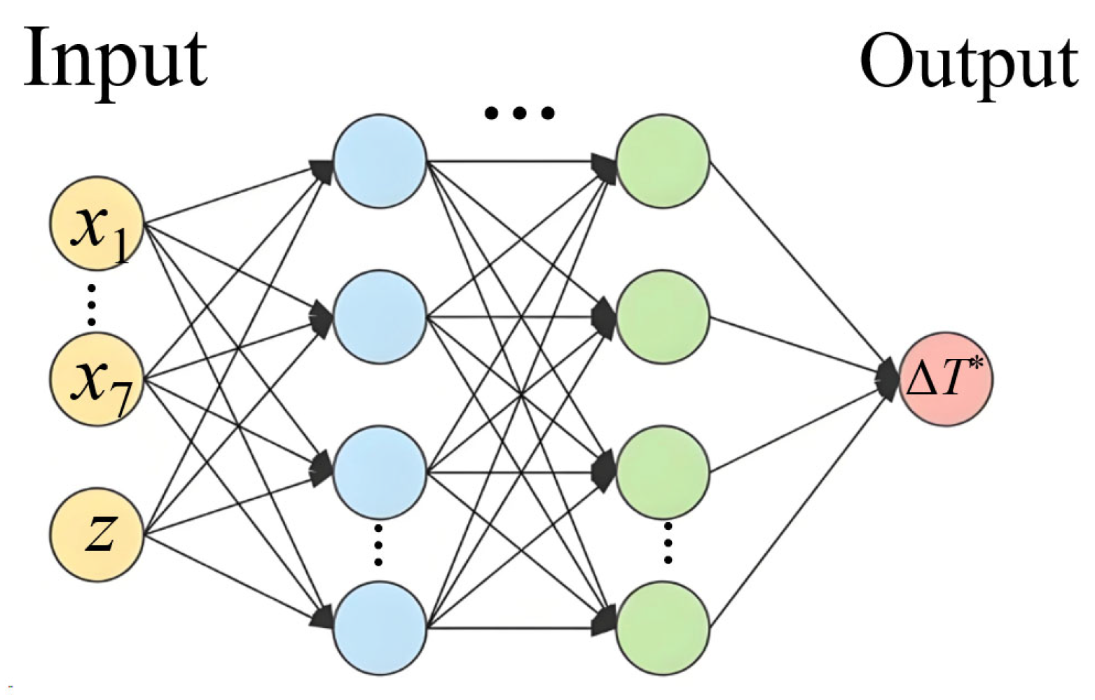The dataset utilizes the results from Section 3.1. Data points are sampled at 1 mm intervals along the flow direction for each simulation case, yielding approximately 20,000 data points. 90% of these are used as the training set and 10% as the test set to train a neural network with 8 inputs (7 quantitative arrangement parameters and 1 streamwise position parameter) and 1 output (local ΔT*). This model is used to compute the streamwise distribution of ΔT* for each case. The fitness (ΔT*_max) for a given arrangement is then determined by comparing all local ΔT* values along the flow direction for that arrangement. Upon completion of training, the R² values for both the validation and test sets exceed 0.999, prompting early stopping and confirming model convergence. 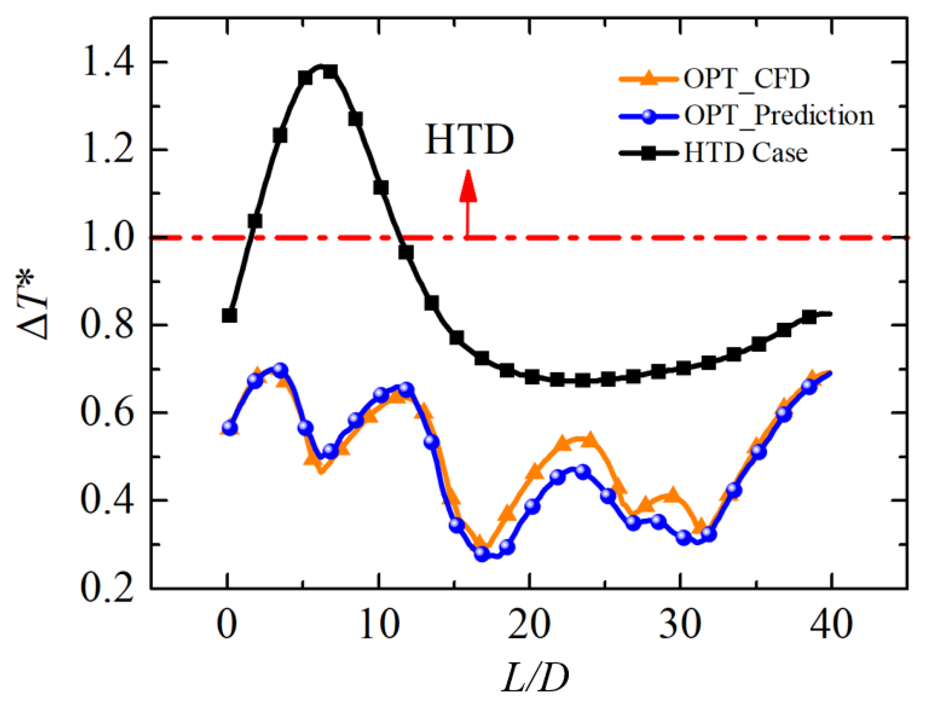Model validation is shown in Figure 9, where an unseen configuration (i.e., not encountered during training) is used, indicating reasonable generalization ability.

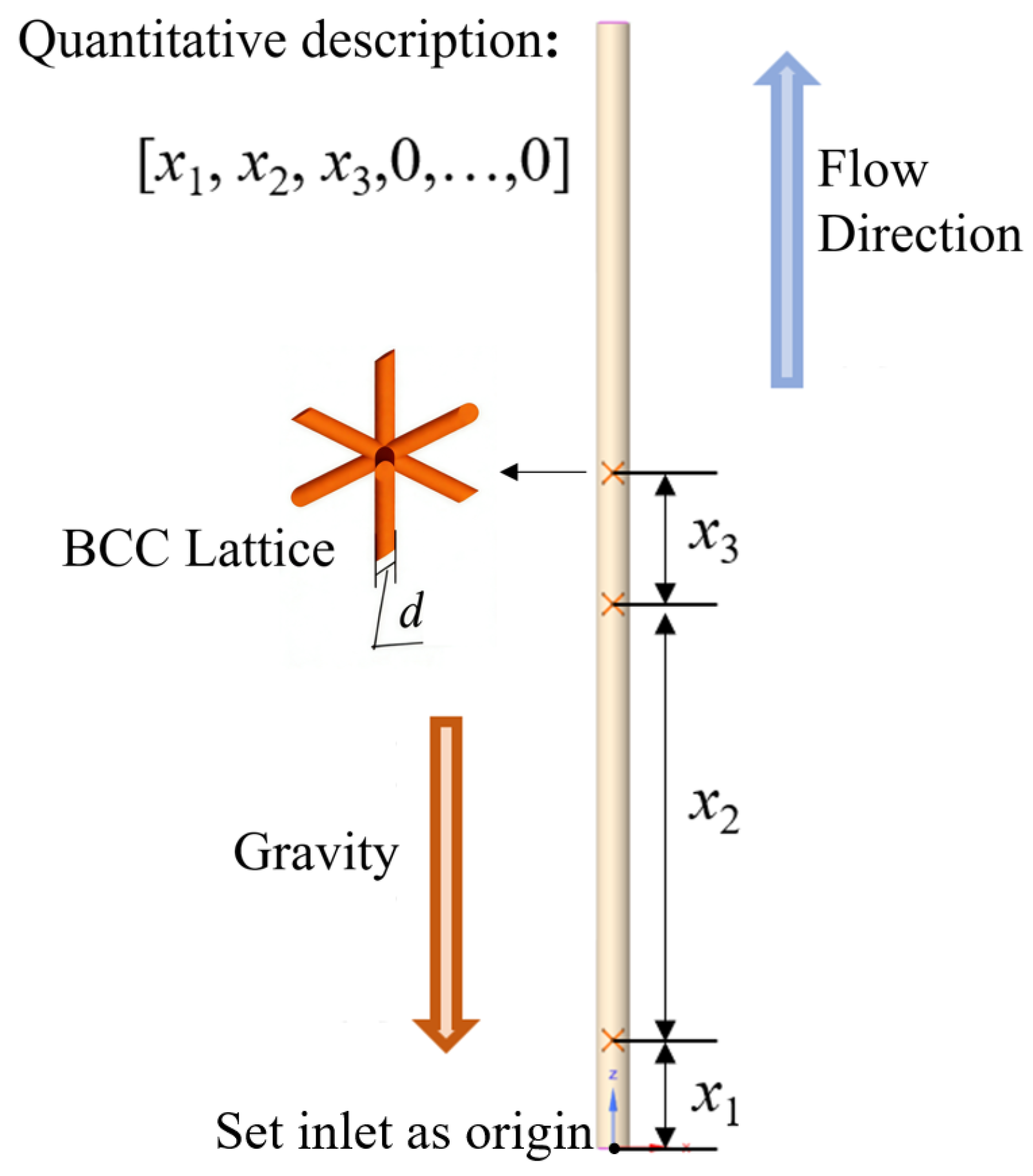
Taking the case with 5 BCC lattice structures as an example, the GA is employed to search for the arrangement that minimizes ΔT*_max. Real-number encoding, random-position crossover, and Gaussian mutation are employed in the genetic algorithm. For the optimization of five BCC structures, in addition to the geometric constraints described in Section 2.1, the conditions x₆ = x₇ = 0 must be satisfied. These two variables are therefore fixed at zero and excluded from the evolution process, effectively reducing the dimensionality of the optimization problem. The genetic algorithm was configured with a constant population size of 500 over 50 generations. For crossover, a random-position single-point scheme is used: for each pair of parent individuals, a crossover point is uniformly selected along the gene length, and the offspring inherit genes from the two parents on either side of this point. The crossover probability is set to 1.0, meaning all offspring pairs undergo crossover. Mutation is performed using a Gaussian operator: for every offspring individual, a randomly selected gene is perturbed by adding a normally distributed random value with zero mean and a standard deviation of 5% of the variable range, followed by clipping to the feasible bounds from 10 to 50 for the active variables. The mutation rate is 1.0 per individual. Selection is based on fitness ranking, favoring individuals with lower objective values. A population size of 500 was chosen following preliminary trials to balance computational efficiency and solution quality while avoiding premature convergence. Convergence was monitored via the best fitness value, which stabilized well before the final generation. The optimization terminates when the optimal solution exhibits minimal change over successive generations. To avoid local optima, the entire process was repeated three times, producing consistent results. Therefore, it is concluded that an optimal spatial arrangement exists for 5 BCC lattice structures under the given conditions, and the optimal arrangement is: [34.9, 54.1, 11.6, 56.6, 29.9, 0, 0]. To verify the accuracy of the prediction, CFD simulations were conducted for this optimal arrangement to obtain its heat transfer characteristics. As shown in Figure 9, the black curve represents the HTD condition in a smooth tube, where regions with ΔT* > 1.0 are considered to be in a state of HTD. In contrast, the optimized result completely suppresses HTD, with a maximum ΔT*_max of 0.69. Furthermore, the model’s prediction shows good agreement with the CFD results, with a maximum error of approximately 8.8%. Since the optimal arrangement did not appear in either the training or test sets, this also demonstrates the reliability of the predictive deep learning model. Compared to the average ΔT*_max of random arrangements, the optimization result shows an improvement of 38.86% and completely eliminates the HTD phenomenon.

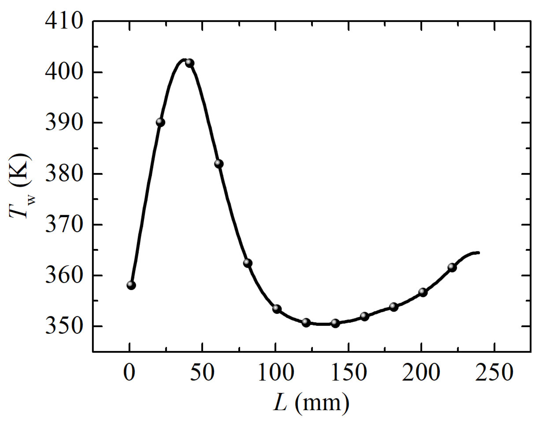
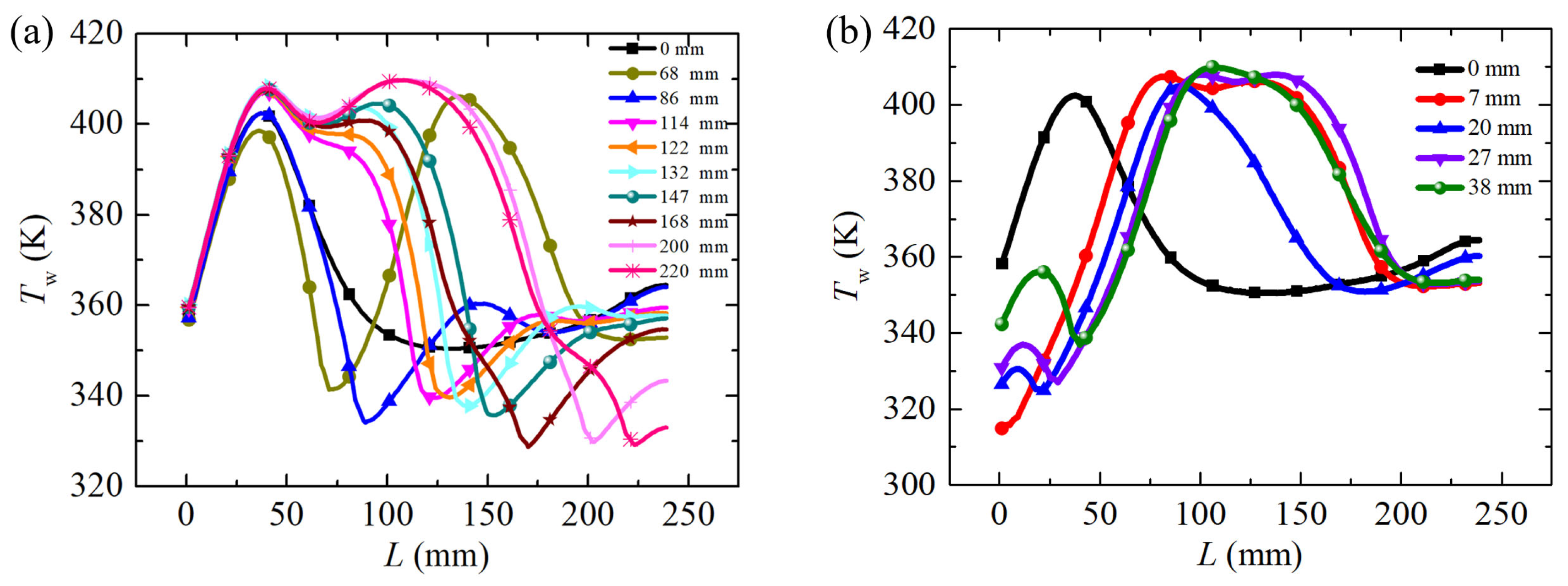
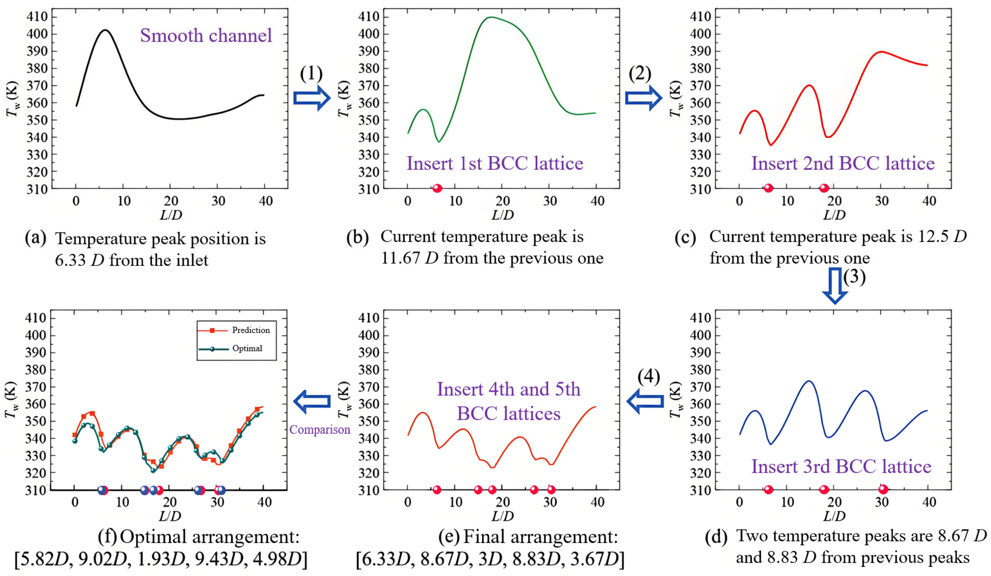
The positional relationship between the optimal arrangement and the HTD temperature peak was further analyzed. It can be inferred that placing BCC structures sequentially upstream of each temperature peak could yield a favorable arrangement. To quantitatively analyze the relationship between the optimal arrangement and the positions of individual temperature peaks, a step-by-step CFD analysis was performed by adding BCC structures one by one, as illustrated in Figure 10. After obtaining the wall temperature distribution for the smooth tube (a), the first BCC structure was placed at the location of the temperature peak (marked in red on the axis). A second CFD simulation was then conducted for the channel with one BCC structure to obtain the new wall temperature distribution (b) and identify the new temperature peak position, where the second BCC was inserted. This process was repeated through multiple CFD simulations, inserting BCC structures at each identified temperature peak, resulting in a predicted arrangement: [6.33 D, 8.67 D, 3 D, 8.83 D, 3.67 D]. Comparing this to the optimal arrangement [5.82 D, 9.02 D, 1.93 D, 9.43 D, 4.98 D] (marked in blue in subplot (f)), the discrepancy is relatively small. However, considering the significant computational cost and complexity of obtaining the optimal arrangement, an approximate optimal arrangement rule can be derived by correcting the predicted arrangement.

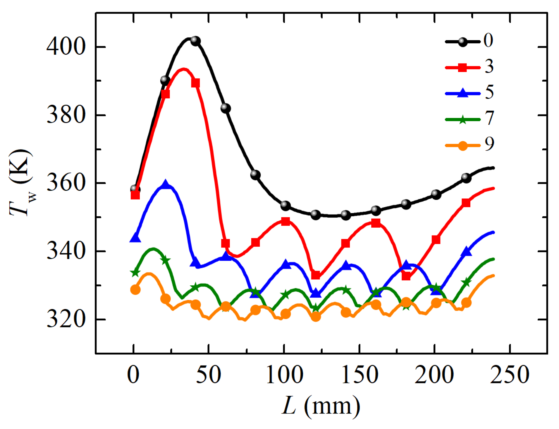
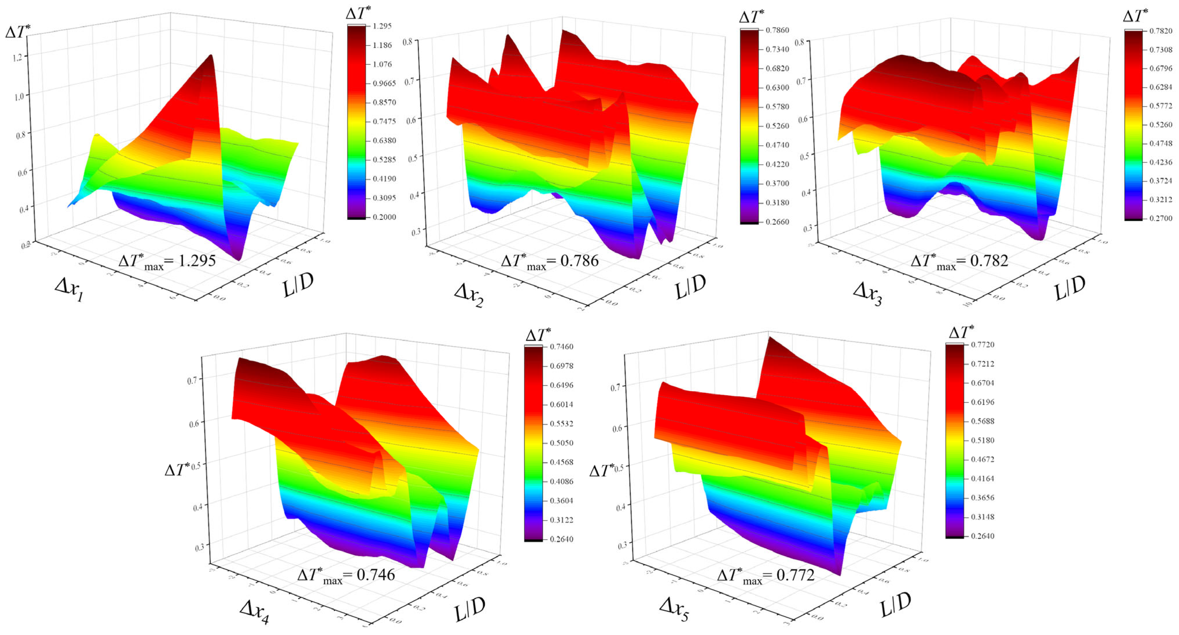
Comparing the two results suggests a corrected rule: insert BCC lattice structures at 0.5–2 D upstream of each identified temperature peak. Even so, obtaining an approximate optimal arrangement requires conducting CFD simulations a number of times equal to the number of BCC structures. To explore whether a simpler design method exists, an input sensitivity analysis was performed based on the optimal arrangement results. As shown in Figure 11, while keeping the other four inputs of the optimal arrangement fixed, the positions of the first, second, third, fourth, and fifth BCC structures (Δx₁~Δx₅) were varied individually to observe the corresponding changes in relative temperature difference along the flow direction. The results indicate that only the change in the position of the first BCC structure leads to a significant variation in ΔT*, even exceeding 1.0 and causing HTD. Although changes in the positions of subsequent BCC structures result in different ΔT* distributions, their impact on the maximum ΔT* is relatively minor. Therefore, to design a simplified arrangement with performance close to the approximate optimal one at a lower computational cost, one can consider placing the first BCC structure at 0.5~2 D upstream of the HTD temperature peak in the smooth channel (as per the approximate optimal design rule above), while distributing the remaining BCC structures uniformly within the channel section between the first BCC structure and the outlet. The underlying flow physics can be summarized as follows: at the leading edge of a BCC structure, an impinging flow generates reverse horseshoe-shaped vortices that enhance local mixing. At the trailing edge, flow separation produces a streamwise vortex that extends far downstream, persistently increasing turbulence intensity. Moreover, at ligament intersections, longitudinal vortex pairs induce secondary flows that enhance radial mixing between the bulk fluid and the boundary layer, thereby weakening the buoyancy effect—the primary driver of heat transfer deterioration (HTD). These mechanisms explain why placing the first BCC structure within 0.5–2 D upstream of the expected temperature peak is critical: it disrupts the developing deterioration before the peak forms, and the induced vortices sustain improved mixing downstream. For more details, see ref. [28].

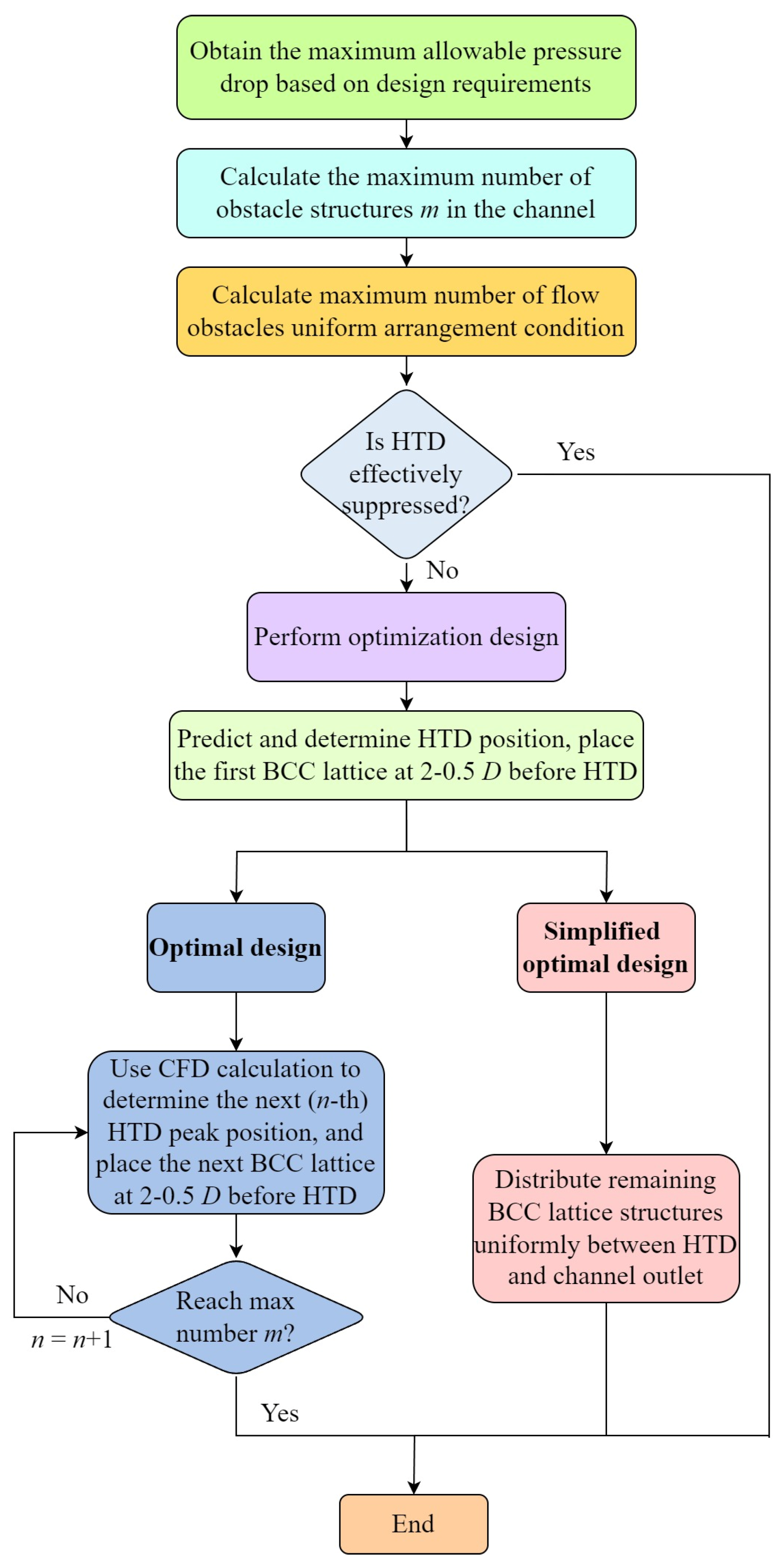
Figure 12 summarizes the arrangement design methodology proposed in this chapter. First, determine the maximum allowable number of BCC structures within the channel based on design requirements, and test whether a uniform arrangement can effectively suppress HTD (i.e., achieve ΔT*_max < 1.0). If a uniform arrangement fails to suppress HTD, optimization design should be considered. If the goal is to obtain an HTD-suppressing arrangement with relatively low computational cost, a simplified design can be adopted, focusing primarily on the placement of the first BCC structure while arranging the remaining structures uniformly. If an approximate optimal arrangement is desired, the position of each BCC structure needs to be considered.

It is important to note that the proposed design methodology, including the 0.5–2 D placement rule and the simplified design flowchart, is derived based on the specific baseline configuration and operating conditions investigated in this study. While the validation case under different operating conditions in Section 3.3 demonstrates the potential applicability of this approach, the current evidence is limited to a relatively narrow parameter range. Therefore, the proposed design strategy should be regarded as a case-supported engineering heuristic for rapid preliminary design rather than a universally validated methodology. When applied to significantly different geometries or operating conditions, further verification through numerical simulation or experimental testing is recommended to ensure the effectiveness of the design.

3.3. Validation of the Proposed Design Methodology

To validate the reliability of the optimization design methodology, a different operating condition case was randomly selected to verify its effectiveness in suppressing HTD. As shown in

Table 6. Comparison between the prior working conditions and the validation working conditions.

	Baseline Working Condition	Validation Working Condition
Tin	295 K	301.15 K
P	7.8 MPa	8.0 MPa
G	320 kg/(m2·s)	385 kg/(m2·s)
q	60 kW/m2	31.7 kW/m2
D	6 mm	6 mm
d	0.1 D	0.1 D
L	40 D	110 D

, the selected validation conditions differ from the previously used design conditions, allowing for an assessment of the generalizability of the proposed method.

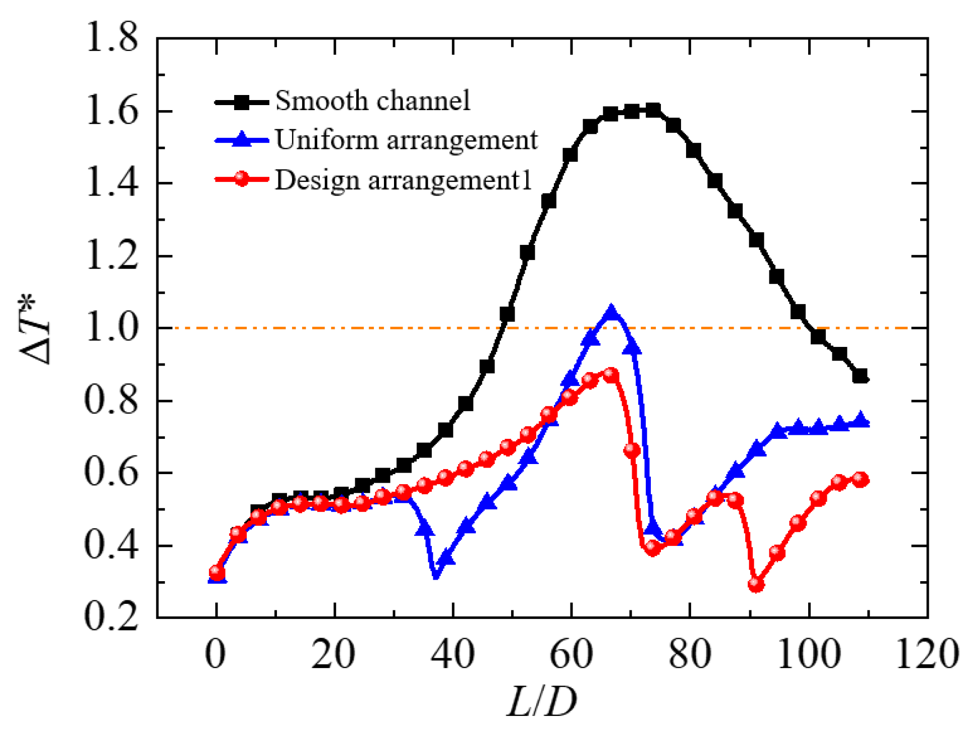
First, the simplified design method is verified. As shown in Figure 13, assuming the pressure drop constraint only allows for two BCC lattice structures, CFD simulation confirms significant HTD occurs in the smooth channel. A uniform arrangement of the two structures fails to effectively suppress HTD, indicating the need for an optimized design to achieve HTD suppression with a limited number of BCC lattices. The simplified design process requires obtaining the heat transfer characteristics and the temperature peak location of the smooth channel only. The first lattice structure is placed 1 D upstream of the temperature peak position, and the second BCC structure is placed at the midpoint between the first BCC structure and the channel outlet. CFD results, represented by the red curve in the figure, demonstrate that the layout obtained by the simplified design method effectively suppresses HTD.

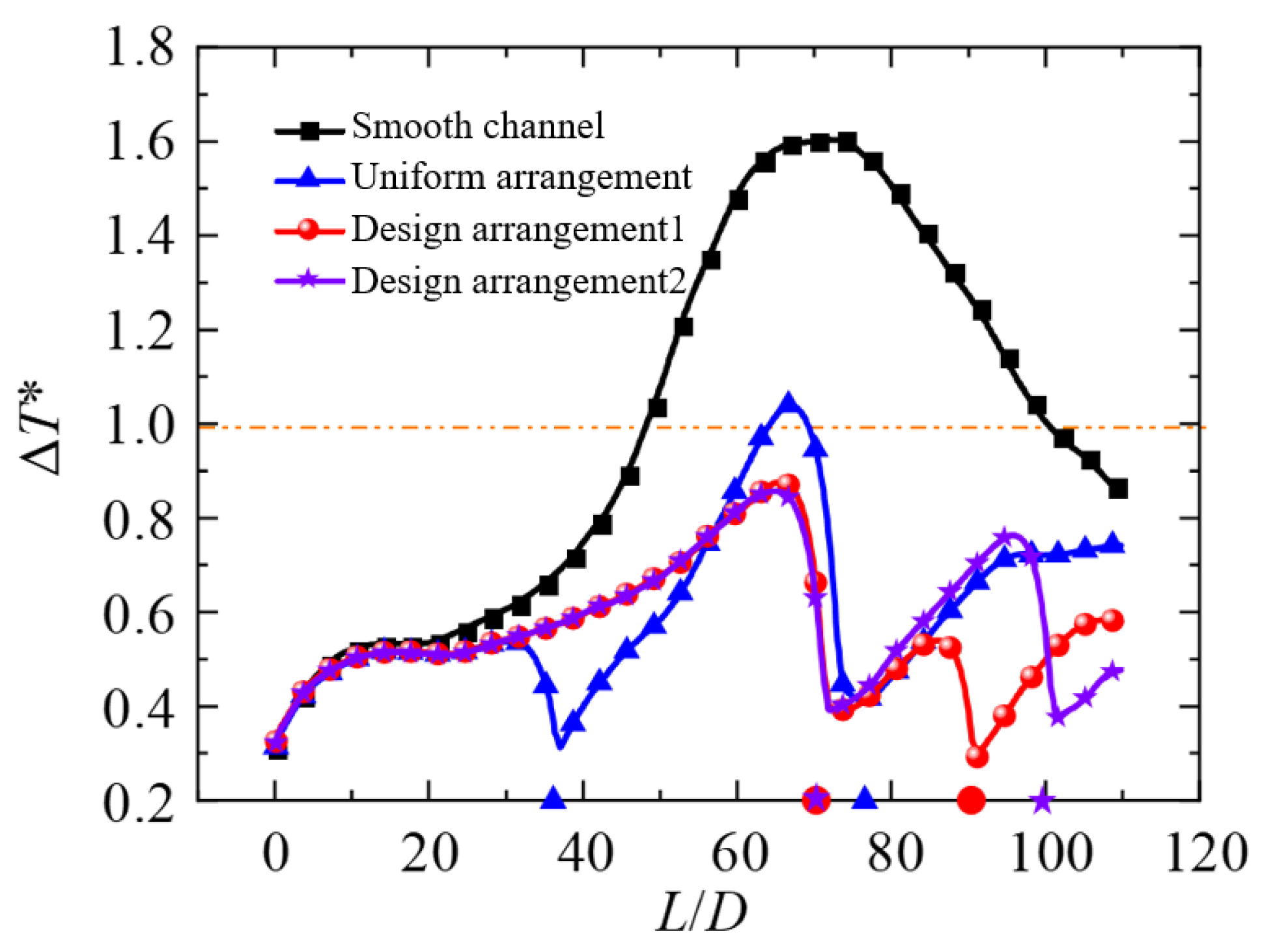
Subsequently, validation of the approximate optimal design methodology was carried out. As illustrated in Figure 14, a comparison is presented between the approximate optimal arrangement (Design Arrangement 2) and the simplified design arrangement (Design Arrangement 1). The approximate optimal arrangement was derived through the iterative process outlined in Figure 10, which involved sequentially inserting BCC lattice structures and performing CFD simulations. Following the placement of the first BCC structure at a location 1 D upstream of the initial temperature peak in the smooth channel, an initial CFD simulation was conducted. The resulting temperature field identified the position of the second temperature peak, guiding the placement of the second BCC structure at 2 D upstream of this secondary peak. A final CFD simulation was then performed, yielding the temperature distribution marked by the purple curve in Figure 14. The corresponding streamwise placement (L/D) for each design is indicated by markers on the horizontal axis. The comparison reveals that the approximate optimal arrangement achieves a marginally lower ΔT*_max than the simplified design. Importantly, both designs successfully suppress heat transfer deterioration entirely and maintain the temperature distribution within a significantly lower range. Consequently, either the approximate optimal arrangement or the simplified design can be selected based on specific application requirements.

Although the validation case presented in this section confirms the effectiveness of both the simplified and approximate optimal design methods under an alternative operating condition, it should be emphasized that this represents only a single additional data point. The generalizability of the proposed design guidelines to a broader range of operating parameters, including extreme conditions far from the critical point, significantly different mass fluxes, or varying heat flux distributions, remains to be further investigated. Future studies involving a more comprehensive parametric matrix would be valuable to strengthen the statistical confidence in the proposed design heuristics.

4. Conclusions

This study presented an investigation into the design and optimization of spatial arrays for BCC lattice structures to suppress heat transfer deterioration (HTD) in supercritical CO₂ flows within a circular channel and to find effective optimization designs. Through numerical analysis and the hybrid deep learning-genetic algorithm framework, the following key conclusions are drawn:

(1)

The axial placement of a BCC lattice relative to the inherent HTD temperature peak is critical. Positioning a lattice upstream of the peak provides effective local heat transfer enhancement but primarily results in a downstream shift of the deterioration zone. Placing a unit significantly downstream of an established peak fails to suppress the upstream HTD and may only induce a localized, heat transfer improvement followed by recurrent deterioration. Therefore, proactive intervention upstream of the deterioration region is essential.

(2)

For a fixed number of BCC lattices, the specific non-uniform spatial array has a profound and decisive influence on the efficacy of HTD suppression, quantified by the maximum dimensionless temperature difference (ΔT*_max). In contrast, the influence of the array on the overall pressure drop (and thus friction factor f) for a given unit count is negligible. Its effect on the area-averaged Nusselt number (Nu_ave) is moderate but secondary. Consequently, under a fixed BCC count constraint, the optimization objective should focus directly on minimizing ΔT*_max.

(3)

A design methodology for HTD suppression has been established and preliminarily validated under the investigated conditions. The core principle involves the placement of BCC units upstream of developing wall temperature peaks. Two practical implementation strategies are provided: the simplified design method offers a computationally efficient approach suitable for rapid preliminary design, while the approximate optimal method provides improved performance at higher computational cost. Both methods demonstrated reliable HTD suppression within the tested parameter range. However, it should be noted that the proposed 0.5–2 D placement rule and the design flowchart are engineering heuristics derived from limited operating conditions; their applicability to significantly different geometries or operating parameters requires further verification.