Distributed Co-Simulation of Reinforcement Learning Optimized Fuzzy PID Control of a 10-MW Wind Turbine Yaw System

Abstract

To address the limited adaptability and tuning efficiency of conventional yaw controllers under turbulent wind conditions, this paper investigates a reinforcement learning (RL)–optimized fuzzy PID control scheme for offshore wind turbine yaw systems. A distributed real-time co-simulation framework is established, in which a high-fidelity OpenFAST wind turbine model is coupled with a Simulink-based controller via networked data exchange to reflect realistic sampling and communication constraints. The proposed controller is examined under IEC 61400-1–compliant normal and extreme turbulence wind scenarios and is compared with conventional PID, fuzzy PID, particle swarm optimization (PSO)–based fuzzy PID, gray wolf optimizer (GWO)–based fuzzy PID, and model predictive control (MPC) schemes. Simulation results indicate that the proposed method reduces yaw rate root mean square (RMS) by up to 40% and total yaw energy consumption by up to 41%, while maintaining yaw alignment accuracy under both operating conditions.

1. Introduction

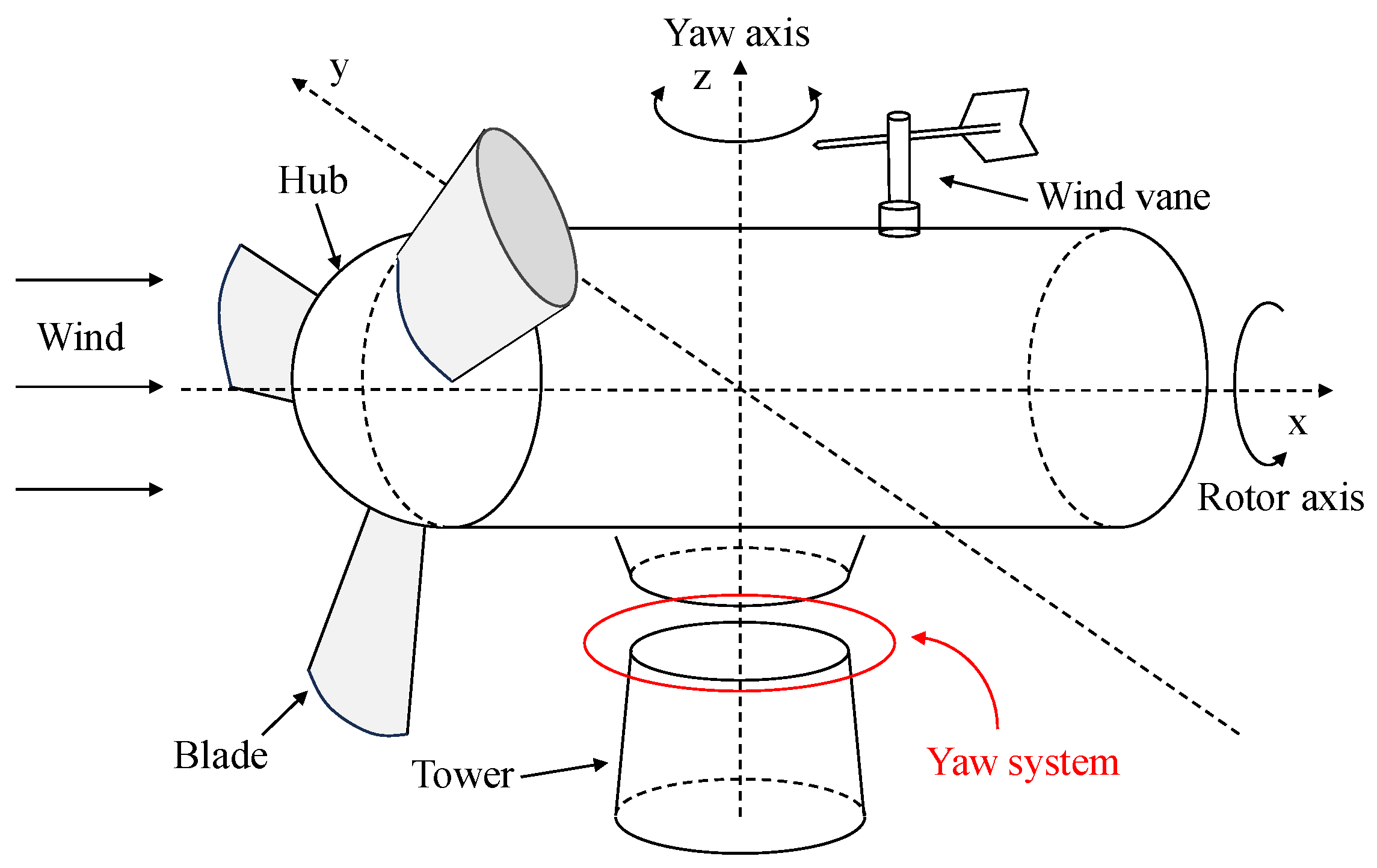
Efficient yaw control is essential for modern offshore wind turbines because it directly affects aerodynamic power capture, asymmetric load distribution, and long-term actuator usage. As wind turbines develop toward the multi-megawatt scale, with larger rotor diameters, higher yaw moments, and stronger aeroelastic coupling, yaw control must balance energy capture, load mitigation, control smoothness, and actuator lifetime under nonlinear and highly disturbed operating conditions. A recent state-of-the-art review on horizontal axis wind turbine(HAWT) control [1] pointed out that, with increasing turbine size and flexibility, wind turbine control should address power regulation, fatigue attenuation, reliability, and availability in an integrated manner, rather than focusing only on power maximization. To clarify the physical structure discussed in this study, the schematic diagram of the wind-turbine yaw system is shown in Figure 1.

Compared with pitch and torque control, yaw control is mainly driven by wind-direction variation and therefore remains relevant throughout the turbine operating envelope. Its purpose is to maintain rotor–nacelle alignment with the incoming wind, thereby reducing yaw-misalignment and associated power loss while avoiding excessive nacelle motion, oscillatory response, and unnecessary wear of motors, gears, and bearings. In this context, active yaw control has long been recognized as a critical subsystem in MW-class wind turbines. Choi et al. [2] investigated active yaw control for an MW-class wind turbine, Elkodama et al. [3] analyzed the yaw-control characteristics of a twin-rotor 10 MW wind turbine, Hu et al. [4] proposed a power-loss-based yaw strategy to improve power capture while reducing yaw-action frequency. These studies indicate that yaw control should be viewed not only as an alignment problem, but also as a trade-off among energy performance, load-related behavior, and actuator burden.

Existing yaw-control studies have gradually evolved from rule-based engineering strategies toward more adaptive and intelligent approaches. In conventional practice, yaw-system design often relies on yaw-error thresholds, delay logic, operating modes, or adaptive yaw-speed scheduling. Representative studies have examined yaw-error optimization [5], yaw strategies based on turbulence intensity and operating modes [6], and adaptive yaw-speed schemes using lookup structures [7]. The main advantage of such methods lies in their simplicity, low computational cost, and ease of practical implementation. However, their performance remains strongly dependent on fixed rules or manually selected thresholds, which limit adaptability under rapidly varying wind direction and stochastic turbulence.

To improve robustness under nonlinear and uncertain conditions, fuzzy and fuzzy-PID-based yaw-control approaches have also been explored. Theodoropoulos et al. [8] developed a fuzzy regulator for wind-turbine yaw control, and Torabi et al. [9] further studied fuzzy control for a noisy wind-turbine yaw system. These studies showed that fuzzy control can better accommodate disturbance and nonlinear behavior than purely fixed-gain logic. Nevertheless, the performance of such methods still depends heavily on the design of membership functions, rule bases, quantization factors, and scaling parameters, which are often selected empirically. Therefore, although fuzzy yaw control offers greater flexibility than conventional rule-based strategies, its applicability across different wind regimes and operating conditions remains limited by parameter-design subjectivity.

To reduce this empirical tuning burden, optimization-based yaw-parameter design has also been investigated. Song et al. [10] optimized yaw-control parameters to improve the power-extraction efficiency of HAWT. Such studies confirm that intelligent or heuristic optimization can improve yaw-control parameter selection. However, such approaches are generally carried out offline, and the resulting parameter sets remain fixed after tuning. Their performance may therefore deteriorate when the operating environment changes significantly. Moreover, direct studies combining wind-turbine yaw control with optimization-assisted fuzzy-PID parameter design remain limited, especially for large offshore wind turbines evaluated under high-fidelity aeroelastic simulation conditions.

In parallel, advanced yaw-control studies have introduced prediction-based and data-driven mechanisms. Hure et al. [11] reported an optimal yaw-control strategy supported by very short-term wind predictions, Chen et al. [12] proposed an LSTM-NN-based yaw-control method using upstream wind information. For yaw-misalignment correction, Bao and Yang [13] developed a data-mining compensation approach, while Bao et al. [14] further proposed a data-driven method for identifying and compensating inherent yaw-misalignment. These studies show that yaw-control research has gradually moved from static rule logic toward prediction-assisted and data-driven decision making. However, most of these methods focus on misalignment estimation, compensation, or predictive yaw-command generation, rather than on learning-assisted tuning of a lightweight engineering controller.

Among recent intelligent methods, RL provides a promising route for yaw-control improvement under stochastic wind conditions. Saenz-Aguirre et al. [15] proposed an artificial-neural-network-based RL method for wind-turbine yaw control, in which a Q-learning-derived control policy was combined with ANN representation to alleviate large Q-matrix management issues. More recently, Puech and Read [16] developed an improved RL-based yaw-control algorithm that explicitly balances yaw-misalignment reduction and yaw usage. These studies demonstrate the potential of RL for yaw control and show that learning-based methods can improve the trade-off between alignment performance and actuation economy. However, most existing RL-related studies focus on direct yaw-decision learning rather than using RL as an engineering-oriented offline tuner for a lightweight fuzzy-PID controller. In addition, many of these studies rely on simplified simulation environments and do not explicitly consider networked signal exchange, timing constraints, or IEC-compliant turbulent wind excitation.

At the validation-platform level, recent studies have increasingly emphasized real-time, hybrid, and co-simulation environments for wind-energy systems. Sadraddin and Shao [17] proposed a distributed real-time hybrid simulation method for dynamic-response evaluation of floating wind turbines, while Qu et al. [18] developed a real-time aero-elastic-electrical co-simulation platform with hardware-in-the-loop implementation for a PMSG wind turbine. These studies highlight the importance of evaluating advanced control strategies in environments that reflect coupled dynamics, practical timing behavior, and implementation-oriented constraints, rather than relying only on simplified stand-alone simulation models. Nevertheless, such platform-oriented studies are rarely combined with RL-assisted tuning of fuzzy-PID yaw controllers for large offshore wind turbines.

Taken together, the existing literature shows that yaw control has evolved from rule-based active alignment to fuzzy regulation, optimization-assisted parameter design, prediction-assisted decision making, and RL based strategies. However, an important gap still remains for large offshore wind turbines. Existing studies mainly focus on direct yaw-decision logic, yaw-misalignment diagnosis, or prediction-based compensation, whereas high-fidelity real-time or co-simulation studies are seldom integrated with the learning-assisted tuning of fuzzy-PID yaw controllers under IEC-compliant turbulent inflow conditions. Therefore, rather than pursuing end-to-end deep RL control, the present work develops a tabular Q-learning-assisted offline tuning framework for a fuzzy-PID yaw controller, so that the online control layer remains lightweight and interpretable while the parameter design benefits from simulation-guided learning in a high-fidelity distributed OpenFAST–Simulink co-simulation environment.

Based on this motivation, the main contributions of this paper are as follows:

(1)

A distributed OpenFAST-Simulink co-simulation framework is established for yaw-control evaluation, incorporating networked bidirectional data exchange, asynchronous execution, and practical timing constraints.

(2)

A tabular Q-learning-assisted offline tuning strategy is developed to optimize the quantization and scaling parameters of the fuzzy-PID controller in a discretized five-dimensional parameter space.

(3)

Comprehensive operating-condition testing is conducted on the co-simulation platform using IEC-compliant high-fidelity models, including the OpenFAST turbine model and TurbSim 3-D turbulent wind fields.

The remainder of this paper is organized as follows: Section 2 presents the wind-turbine yaw-system model, the fuzzy-PID controller, the tabular Q-learning-based tuning method, and the distributed co-simulation framework. Section 3 reports the comparative simulation results. Section 4 and Section 5 present the discussion and conclusions, summarize the main findings of this study, and outline future work.

2. Materials and Methods

2.1. Modeling of the Multiphysics-Coupled Nonlinear System

2.1.1. Multiphysics-Coupled Co-Simulation Architecture

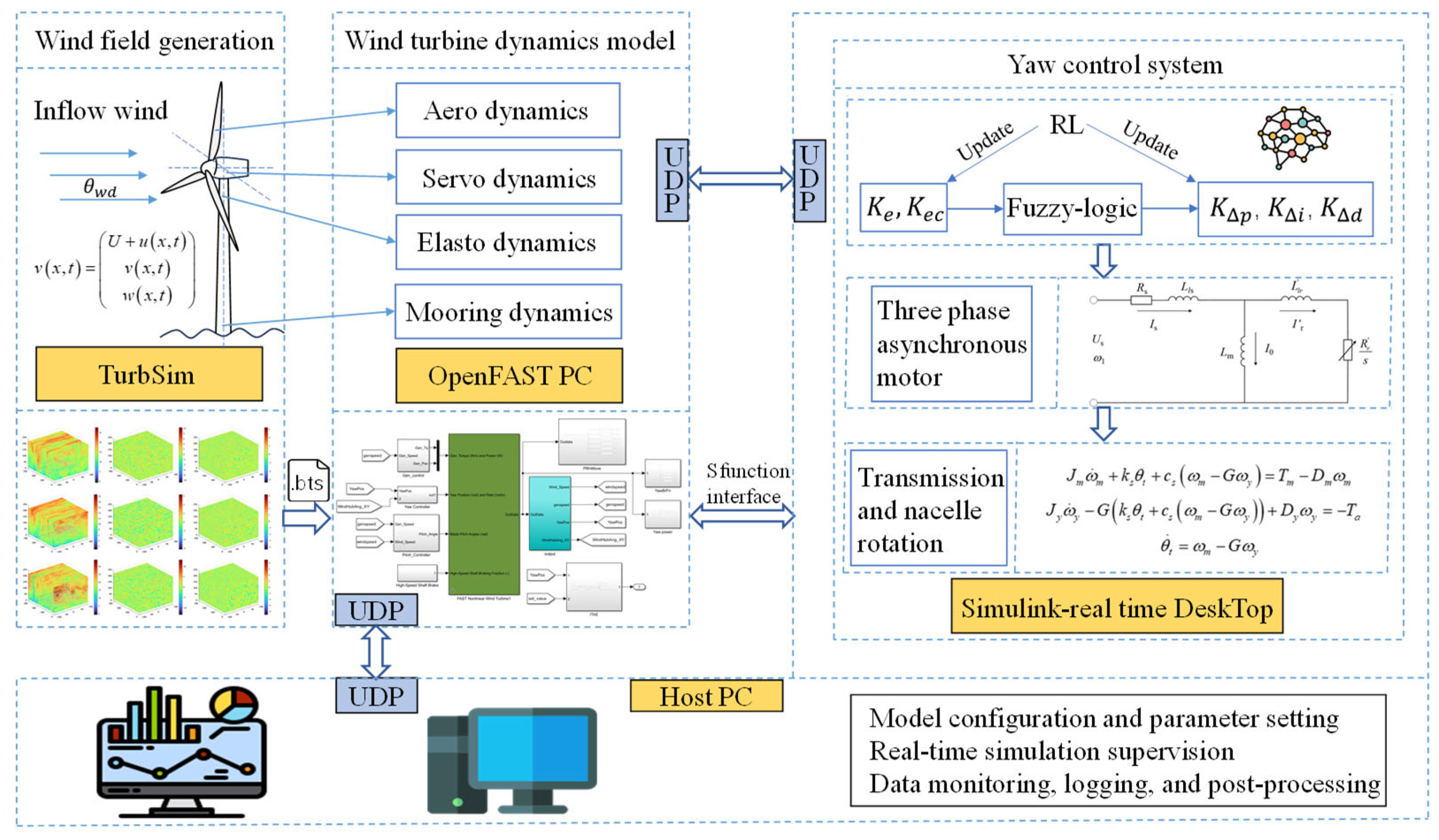
To comprehensively evaluate yaw control performance under realistic operating conditions, a high-fidelity Multiphysics co-simulation framework is established, integrating three-dimensional turbulent wind field generation, aeroelastic wind turbine modeling, and closed-loop yaw control within a unified architecture, as shown in Figure 2. The framework consists of three tightly coupled subsystems: TurbSim for stochastic turbulent wind-field generation and OpenFAST for aero-hydro-servo-elastic wind turbine simulation, both developed by the National Renewable Energy Laboratory (Golden, CO, USA) [19], and Simulink for controller implementation and closed-loop integration, developed by MathWorks (Natick, MA, USA).These subsystems jointly enable accurate representation of wind–structure–control interactions through low-latency bidirectional data exchange.

2.1.2. Construction of Three-Dimensional Turbulent Inflow Scenarios in Accordance with IEC 61400-1

To accurately represent the complex atmospheric disturbances affecting yaw control performance, a three-dimensional non-homogeneous turbulent inflow field is constructed in accordance with IEC 61400-1 [20]. The turbulence characteristics are described using the Kaimal spectral model. The wind velocity is expressed as follows:

$$v\left(x,t\right)=\left[\begin{array}{c}U+u\left(x,t\right)\\ v\left(x,t\right)\\ w\left(x,t\right)\end{array}\right]$$

(1)

where U denotes the mean wind speed, and u(x,t), v(x,t), and w(x,t) represent the longitudinal, lateral and vertical turbulent components, respectively.

(1)

Kaimal Turbulence Power Spectral Density (PSD)

For each turbulent component, the one-sided power spectral density at a given height can be expressed as:

$$S_u\left(f\right)={\displaystyle \frac{4{\sigma }_u^2{L}_u/U}{{\left(1+6f{L}_u/U\right)}^{5/3}}}$$

(2)

$$S_v\left(f\right)={\displaystyle \frac{4{\sigma }_v^2{L}_v/U}{{\left(1+6f{L}_v/U\right)}^{5/3}}}$$

(3)

$$S_w\left(f\right)={\displaystyle \frac{4{\sigma }_w^2{L}_w/U}{{\left(1+6f{L}_w/U\right)}^{5/3}}}$$

(4)

where f denotes the frequency, ${\sigma }_i$ is the standard deviation of the i-th component, and L_i is the corresponding integral turbulence length scale.

The turbulence intensity I is defined as $I={\sigma }_u/U$.

(2)

Spatial Coherence and Cross-Spectral Matrix

To account for spatial correlation within the wind field, the coherence function ${\gamma }_{ij}\left(f\right)$ is introduced. A commonly used expression is given by:

$${\gamma }_{ij}\left(f\right)=\exp \left(-C{\displaystyle \frac{f{d}_{ij}}{U}}\right)$$

(5)

where d_ij denotes the distance between two grid points and C is an empirical decay coefficient. Accordingly, the cross-spectral density matrix can be written as:

$$S\left(f\right)=\left[\begin{array}{ccc}{S}_u\left(f\right)& {\gamma }_{uv}\sqrt{S_u\left(f\right)S_v\left(f\right)}& \dots \\ \dots & S_v\left(f\right)& \dots \\ \dots & \dots & S_w\left(f\right)\end{array}\right]$$

(6)

By applying Cholesky decomposition, the following factorization is obtained:

$$S\left(f\right)=H\left(f\right)H^T\left(f\right)$$

(7)

(3)

Generation of Time-Domain Wind Field via Spectral Representation

First, a vector of independent complex Gaussian random variables R(f) is generated. The correlated spectral amplitudes are then computed as follows:

$$G\left(f\right)=H\left(f\right)R\left(f\right)$$

(8)

Finally, the turbulent wind field in time domain is reconstructed by applying the inverse fast Fourier transform (iFFT):

$$v\left(x,t\right)=iFFT\left\{G\left(f\right)\right\}$$

(9)

The resulting wind field is organized into a matrix form:

$$V\left(x,t\right)=\left[\begin{array}{ccc}u\left(x_1,t\right)& \dots & u\left(x_n,t\right)\\ v\left(x_1,t\right)& \dots & v\left(x_n,t\right)\\ w\left(x_1,t\right)& \dots & w\left(x_n,t\right)\end{array}\right]$$

(10)

which describes the three velocity components at n spatial grid points over time.

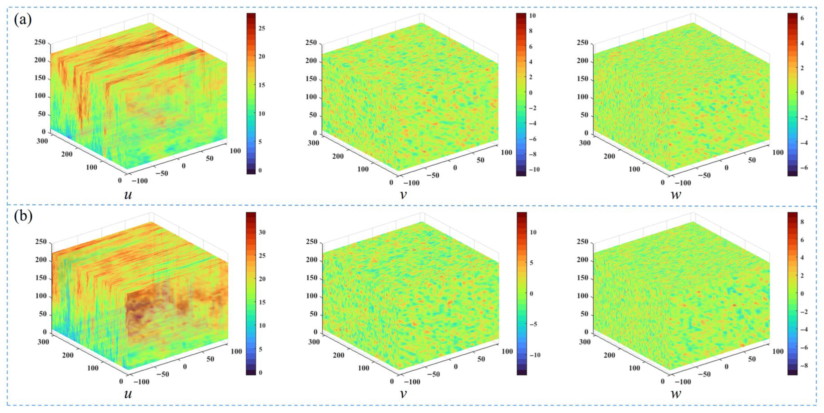
Based on the above procedure, TurbSim is employed to generate IEC 61400-1–compliant turbulent inflow files, which are subsequently incorporated into the OpenFAST–Simulink co-simulation platform. Two representative wind scenarios corresponding to normal and extreme operating conditions are considered in this study, as shown in Figure 3.

2.1.3. Six-Degree-of-Freedom Modeling of the Offshore Wind Turbine

The offshore wind turbine is modeled as a fully coupled nonlinear aero–servo–hydro–mooring system with six degrees of freedom (6-DOFs) [21], namely surge, sway, heave, roll, pitch, and yaw [22].

Based on Blade Element Momentum (BEM) theory, the aerodynamic force acting on each blade element is computed as follows:

$$dT={\displaystyle \frac{1}{2}}\rho V_{rel}^{2}c\left(r\right)\left(C_L\cos \Phi +C_D\sin \Phi \right)dr$$

(11)

where the induced velocity and dynamic inflow are solved iteratively according to momentum conservation.

The tower is modeled as a distributed cantilever beam using modal truncation. The first fore–aft mode dominates the turbine–wind coupling behavior:

$$M_t{\ddot{q}}_t+C_t{\dot{q}}_t+K_t{q}_t=F_{aero}$$

(12)

The low- and high-speed shafts are represented using a two-mass torsional model:

$$J_r{\dot{\omega }}_r=T_a-k_s{\theta }_d-c_s{\dot{\theta }}_d$$

(13)

$$J_g{\dot{\omega }}_g=k_s{\theta }_d+c_s{\dot{\theta }}_d-T_g$$

(14)

To simplify the hydrodynamic environment, calm-water conditions are assumed, while the station-keeping stiffness provided by the mooring lines is retained:

$$F_{moor}=-K_{moor}x$$

(15)

This treatment preserves the accuracy of load transmission among yaw motion, tower response, and structural dynamics.

The yaw actuation subsystem establishes the dynamic relationship between motor torque and nacelle rotation. A reduced-order electromechanical model incorporating the yaw motor, gearbox, shaft stiffness, and nacelle inertia is formulated.

The motor torque dynamics are given by:

$${\dot{T}}_m=-{\displaystyle \frac{1}{{\tau }_m}}{T}_m+{\displaystyle \frac{K_{MA}}{{\tau }_m}}u$$

(16)

The transmission dynamics and nacelle rotation are described by:

$$J_m{\dot{\omega }}_m+k_s{\theta }_t+c_s\left({\omega }_m-G{\omega }_y\right)=T_m-D_m{\omega }_m$$

(17)

$$J_y{\dot{\omega }}_y-G\left(k_s{\theta }_t+c_s\left({\omega }_m-G{\omega }_y\right)\right)+D_y{\omega }_y=-T_a$$

(18)

$${\dot{\theta }}_t={\omega }_m-G{\omega }_y$$

(19)

The yaw kinematic relationship is given by ${\dot{\theta }}_y={\omega }_y$.

By defining the physically interpretable state vector as follows:

$$x={\left[{\theta }_y,{\omega }_y,T_m\right]}^T$$

(20)

The aerodynamic yaw torque is a nonlinear function of yaw-misalignment and is linearized about the operating point using a first-order Taylor expansion. The resulting linearized continuous-time state-space representation of the yaw system is given by:

$$\dot{x}=Ax+Bu,y=Cx+Du$$

(21)

with

$$A=\left[\begin{array}{ccc}0& 1& 0\\ -{\displaystyle \frac{1}{J_y}}{\displaystyle \frac{\partial T_a}{\partial {\theta }_y}}{|}_{{\theta }_y^{*}}& -{\displaystyle \frac{D_y}{J_y}}& {\displaystyle \frac{1}{J_y}}\\ 0& 0& -{\displaystyle \frac{1}{{\tau }_m}}\end{array}\right],B=\left[\begin{array}{c}0\\ 0\\ {\displaystyle \frac{K_m}{{\tau }_m}}\end{array}\right],C=\left[\begin{array}{ccc}1& 0& 0\end{array}\right],D=0$$

(22)

Each state retains a clear physical interpretation, thereby facilitating accurate propagation of structural loads from the drivetrain to nacelle yaw motion.

For real-time yaw control implementation, zero-order-hold (ZOH) discretization is applied with a sampling period of T_s:

$$x\left[k+1\right]=A_{d}x\left[k\right]+B_{d}u\left[k\right]$$

(23)

where $A_d=e^{A{T}_s}$, and $B_d$ is obtained from the standard matrix exponential integral.

To improve computational efficiency in co-simulation, a validated third-order reduced model based on equivalent first-order motor inertia is also adopted during the parametric analysis and controller tuning stages.

2.2. RL-Optimized Fuzzy PID Yaw Control

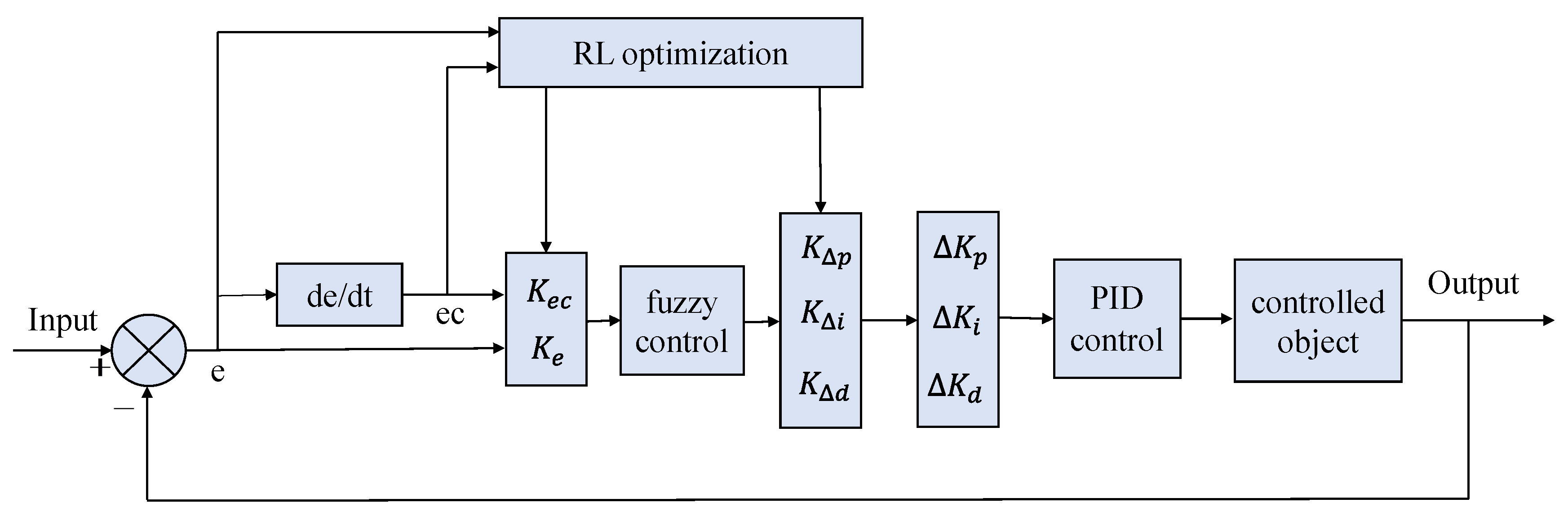
The yaw control scheme for all operating conditions is shown in Figure 4.

2.2.1. Development of the Fuzzy PID Yaw Controller

The fuzzy PID yaw controller uses the yaw tracking error e and its rate of change $\dot{e }$ as the two input variables. These signals are processed through fuzzification, fuzzy inference, and defuzzification to generate three output increments, namely $\mathsf{\Delta }{K}_p$, $\mathsf{\Delta }{K}_i$, and $\mathsf{\Delta }{K}_d$, which are used to adapt the PID gains online [23]. The updated PID parameters are expressed as:

$$K_p=K_{p0}+\Delta K_P$$

(24)

$$K_i=K_{i0}+\Delta K_i$$

(25)

$$K_d=K_{d0}+\Delta K_d$$

(26)

where K_p, K_i, and K_d denote the updated proportional, integral, and derivative gains, respectively, while K_p0, K_i0, and K_d0 denote their initial preset values.

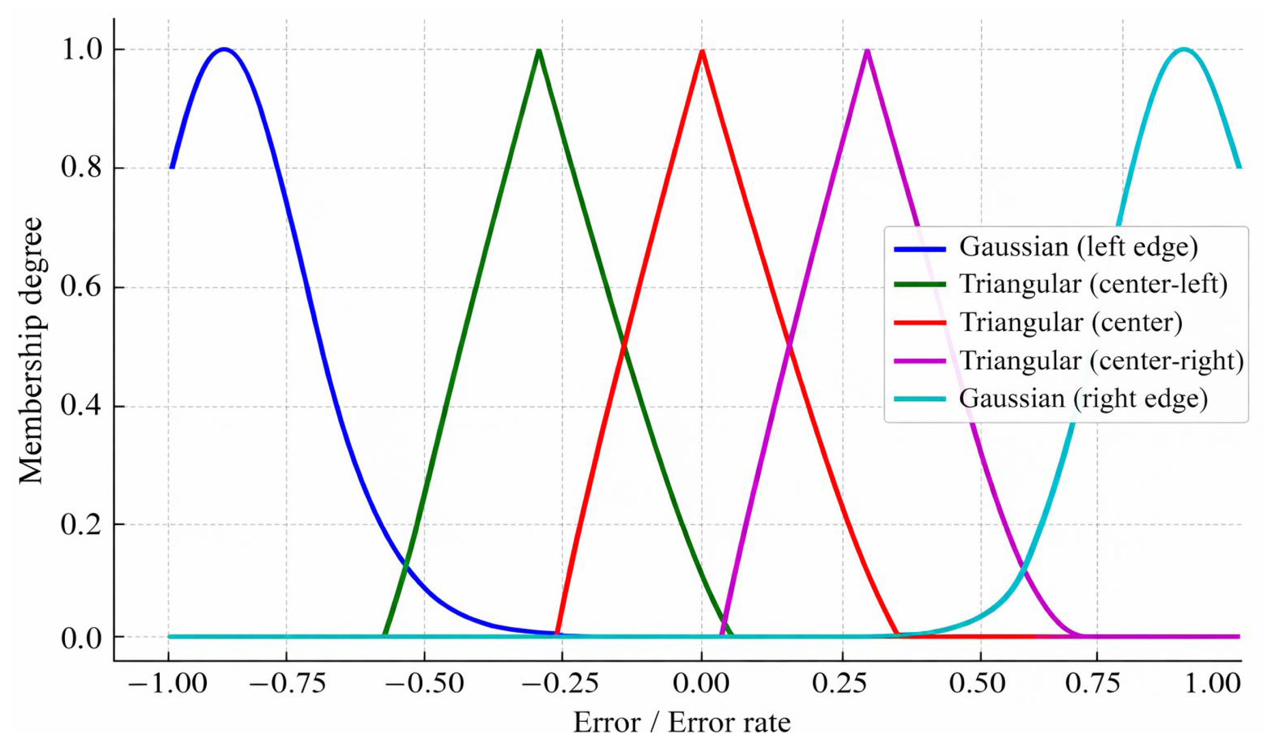
The proposed fuzzy controller employs triangular membership functions in the central region to ensure clear partitioning and computational efficiency, while Gaussian membership functions are adopted near the boundaries to provide smooth transitions under extreme inputs and to avoid abrupt control actions in nonlinear and uncertain operating conditions (Figure 5).

The controller design follows three basic principles:

(1)

For large errors, a relatively high K_p and relatively low K_i and K_d are adopted to accelerate the transient response.

(2)

For moderate errors, the three gains are balanced to maintain stable dynamic behavior.

(3)

For small errors, K_p is reduced, whereas K_i and K_d are increased to improve steady-state accuracy.

To describe the linguistic states of both the inputs and outputs, seven fuzzy subsets are defined: Positive Big (PB), Positive Medium (PM), Positive Small (PS), Zero (ZO), Negative Small (NS), Negative Medium (NM), and Negative Big (NB) [24]. The full rule set is shown in

Table 1. Fuzzy rule table.

	ec	NB	NM	NS	ZO	PS	PM	PB
e
NB		PB NB PB	PB NB PM	PM NB PS	PS NM ZO	ZO NS NS	NS ZO NM	NM PS NB
NM		PB NM PB	PM NM PM	PS NM PS	ZO NS ZO	NS ZO NS	NM PS NM	NB PM NB
NS		PM NS PB	PS NS PM	ZO NS PS	NS ZO ZO	NM PS NS	NB PM NM	NB PB NB
ZO		PS ZO PM	ZO ZO PS	NS ZO ZO	ZO ZO ZO	PS ZO ZO	PM ZO NS	PB ZO NM
PS		NS PS PS	NM PS ZO	NB PS NS	PS PS ZO	PM PS PS	PB PS PM	PB PM PB
PM		NM PM ZO	NB PM NS	NB PB NM	PM PM ZO	PB PM PS	PB PB PM	PB PB PB
PB		NB PB NS	NB PB NM	NM PB NB	PS PB ZO	PM PB PS	PB PB PM	PB PB PB

.

2.2.2. RL-Based Optimization of Fuzzy PID Parameters

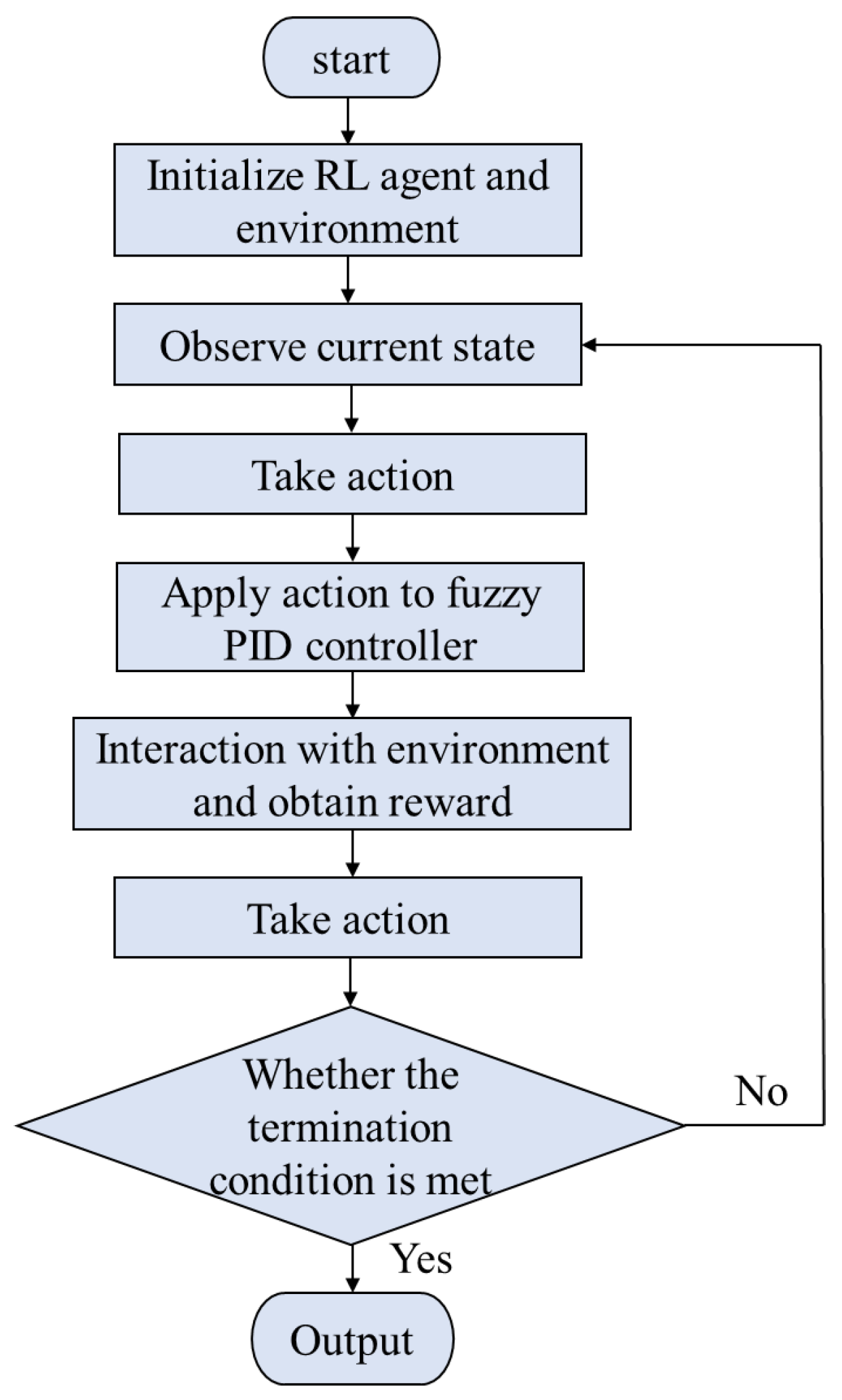
The logic diagram of the proposed RL scheme is illustrated in Figure 6. In this study, RL is not implemented as an end-to-end yaw controller that directly generates continuous control commands. Instead, a tabular Q-learning strategy is employed as an offline parameter-tuning tool to optimize the five key quantization and scaling parameters of the fuzzy PID controller under stochastic wind conditions [15]. This design is motivated by the fact that the optimization target is a bounded low-dimensional parameter vector rather than a high-dimensional continuous control policy. The parameter vector to be optimized is defined as:

$$\theta =\left[K_e,K_{ec},K_{up},K_{ui},K_{ud}\right]$$

(27)

where $K_e$ and $K_{ec}$ denote the input quantization factors associated with the yaw error and its rate of change, respectively, and $K_{up}$, $K_{ui}$, and $K_{ud}$ are the output scaling factors for the proportional, integral, and derivative tuning channels of the fuzzy PID controller. The admissible search ranges of these parameters are given by:

$$L_b=\left[0,0,-0.2,-1,-0.1\right],U_b=\left[15,5,0.1,0.1,1\right]$$

(28)

To enable Q-learning, the continuous five-dimensional parameter space is discretized into a finite state space. In the present implementation, each parameter is uniformly divided into $N_b=10$ levels within its prescribed lower and upper bounds [25]. For the i-th parameter ${\theta }_i\in [L_i,U_i]$, the discretized index is defined as:

$$b_i=clip(round({\displaystyle \frac{{\theta }_i-L_i}{U_i-L_i}}(N_b-1)+1),1,N_b)$$

(29)

where $\mathrm{c}\mathrm{l}\mathrm{i}\mathrm{p}\left(\cdot \right)$ enforces the valid index range. Accordingly, the RL state at time step t is represented as:

$$s_t=\left[b_1,b_2,b_3,b_4,b_5\right],b_i\in \left\{1,2,\dots ,N_b\right\}$$

(30)

And the total number of discrete states is:

$$N_s=N_b^5={10}^5=100,000$$

(31)

In this formulation, the RL state is defined by the discretized parameter vector, whereas the objective function value is used only for reward evaluation. Thus, the learning task is not to discretize the performance index itself, but to search for a better parameter combination within the bounded five-dimensional tuning space.

At each learning step, the agent selects one parameter dimension and one discrete increment from a finite action set. The action is therefore expressed as:

$$a_t=\left(d,\Delta \right),d\in \left\{1,2,3,4,5\right\},\Delta \in \left\{-0.005,-0.002,0,0.002,0.005\right\}$$

(32)

where d denotes the selected parameter dimension and $\mathsf{\Delta }$ is the corresponding parameter increment. As five parameter dimensions and five candidate increments are considered, the action-space size is $N_a=5\times 5=25$. Only one parameter is updated at each step, while the remaining parameters remain unchanged. The corresponding state transition in the parameter space is given by:

$${\theta }_d^{(t+1)}=clip\left({\theta }_d^{(t)}+\Delta ,L_d,U_d\right)$$

(33)

with all non-selected parameters unchanged. Accordingly, the Q-table contains $N_s\times N_a=\mathrm{100,000}\times 25=2.5\times {10}^6$ state–action entries, which remain computationally manageable for offline learning on a PC-based simulation platform.

The discretization granularity was selected as a compromise between search resolution and computational complexity. If too few levels are used, the parameter quantization becomes excessively coarse and weakens the sensitivity of the search process. Conversely, an overly fine discretization would exponentially enlarge the tabular state space and substantially increase the learning burden. For the bounded five-parameter tuning problem considered here, ten levels per dimension provide a practical balance between tuning resolution and computational tractability. Compared with deep RL methods for continuous state and action spaces, the adopted tabular formulation is more appropriate for the present problem because the search space is compact, the parameter bounds are explicit, and end-to-end online policy learning is not required. Under these conditions, tabular Q-learning provides a transparent and sufficiently effective tuning framework without the additional training complexity associated with deep neural approximators.

For each candidate parameter vector $\theta$, the controller performance is evaluated using a simulation-based objective function $J\left(\theta \right)$ computed by the closed-loop co-simulation model [26]. The immediate reward is defined based on the normalized fitness improvement between two consecutive parameter sets:

$$r_t={\displaystyle \frac{J\left({\theta }_t\right)-J\left({\theta }_{t+1}\right)}{\left|J\left({\theta }_t\right)\right|+{\epsilon }_r}}$$

(34)

where ${\epsilon }_r$ is a small positive constant introduced to avoid numerical singularity. A positive reward is obtained when the updated parameter vector reduces the objective function value, whereas a negative reward indicates performance deterioration.

The Q-table is then updated using the standard Bellman recursion:

$$Q\left(s_t,a_t\right)\leftarrow Q\left(s_t,a_t\right)+\alpha \left[r_t+\gamma \underset{a}{\max }Q\left(s_{t+1},a\right)-Q\left(s_t,a_t\right)\right]$$

(35)

where $\alpha$ is the learning rate and $\gamma$ is the discount factor.

In this study, $\alpha =0.1$ and $\gamma =0.9$, and the action-selection policy follow an $\epsilon$-greedy strategy. With probability $\epsilon$, the agent explores by randomly selecting a parameter-dimension/action pair; otherwise, it exploits the current Q-table by choosing the action with the highest Q-value at the current state. To improve the balance between exploration and exploitation [27], the exploration rate is gradually reduced during training as follows:

$${\epsilon }_k=\max \left({\epsilon }_{\min },{\epsilon }_0{\beta }^{k-1}\right)$$

(36)

where $k$ is the episode index, ${\epsilon }_0=0.30$ is the initial exploration rate, ${\epsilon }_{\mathrm{m}\mathrm{i}\mathrm{n}}=0.05$ is the minimum exploration rate, and $\beta =0.92$ is the decay factor. This strategy encourages broader exploration in the early stage of training and more exploitative behavior as learning proceeds.

The training procedure is organized in an episodic manner. In this study, the maximum number of episodes is set to 30, and each episode contains up to 20 parameter-update steps. During training, the best parameter vector encountered so far is retained as the best global solution. In addition, an early-stopping mechanism is introduced so that the training process is terminated when no further improvement in the best fitness value is observed over several consecutive episodes. After training, the optimal parameter vector ${\theta }^{*}$ obtained by Q-learning is fixed and used to construct the final fuzzy PID controller for the subsequent yaw-control co-simulation tests. Therefore, the online control layer remains a conventional fuzzy PID controller, whereas RL is confined to the offline tuning stage.

For benchmark comparison, the initial gains of the conventional PID controller are manually selected as $K_p=0.035$, $K_i=2.5\times {10}^{-3}$, and $K_d=0.1\times {10}^{-7}$. The optimized parameter settings and the main hyperparameters of all compared controllers are summarized in

Table 2. Parameters of each controller.

RL		PSO		GWO		MPC
Parameter	Value	Parameter	Value	Parameter	Value	Parameter	Value
α	0.1	Np	10	N	10	Np	120
γ	0.9	Tmax	30	Tmax	30	Nc	3
β	0.92	w	0.9-0.6	a	2-0	Wy	5
Ns	10	c1, c2	1.2			Wu	0.1
Episodes	30	Vmax	0.5			WΔu	50.5

[28]. In addition, the MPC benchmark is constructed based on the state-space formulation derived in Section 2 [29]. For the representative local MPC controller adopted in this study, the internal prediction model is expressed as

$$G_p(z)=z^{-50}{\displaystyle \frac{1}{37.65z+1}}$$

(37)

The benchmark MPC controller is implemented using MATLAB/Simulink R2024b with the Model Predictive Control Toolbox with a QP-based active-set solver. The online optimization problem is formulated as a constrained finite-horizon quadratic program based on the internal discrete-time yaw prediction model. The stage cost penalizes the output tracking error, the manipulated-variable magnitude, and the manipulated-variable increment:

$$J_{MPC}={\displaystyle \sum _{k=1}^{N_p}{W}_y{e}^2(k)+{\displaystyle \sum _{k=0}^{N_c-1}{W}_u{u}^2(k)}}+{\displaystyle \sum _{k=0}^{N_c-1}{W}_{\Delta u}\Delta u^2(k)}$$

(38)

where $e\left(k\right)$ denotes the yaw tracking error, $u\left(k\right)$ denotes the manipulated variable, and $\mathsf{\Delta }u\left(k\right)$ denotes the control increment. The final MPC settings are selected through preliminary tuning to balance tracking accuracy, control smoothness, and online computational feasibility. More aggressive settings tend to produce excessive yaw actuation, whereas overly conservative settings introduce noticeable response lag due to the delayed predictor structure. Therefore, the adopted parameter set should be understood as a practical engineering compromise for benchmark comparison rather than a configuration optimized for a single performance index only.

2.3. Distributed Co-Simulation Platform Architecture

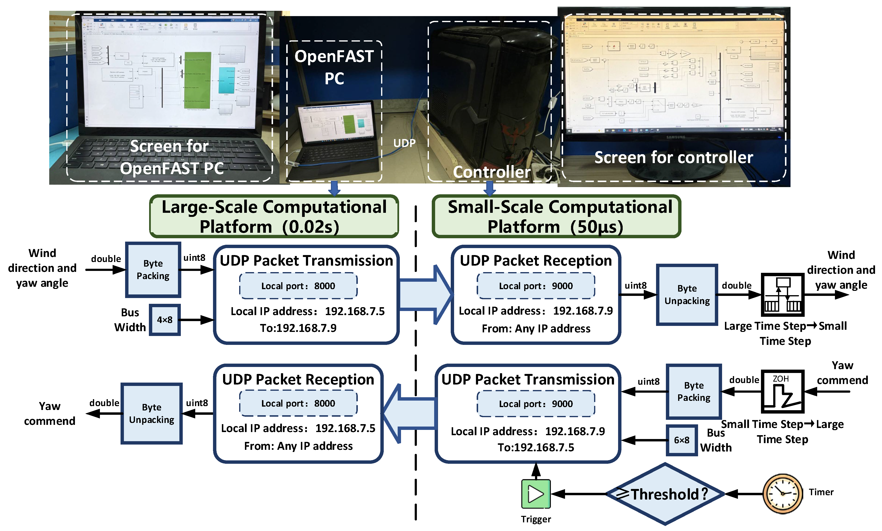
To evaluate the practical feasibility of the proposed yaw control scheme under realistic communication and timing constraints, a distributed PC-based co-simulation platform is established. One computer executes the high-fidelity OpenFAST model as the controlled plant with an integration step of 0.02 s to capture the dominant aeroelastic and mechanical dynamics, whereas the other runs the yaw controller in the Simulink Desktop Real-Time environment with a sampling period of 50 μs to represent high-frequency electrical and control dynamics [30]. The two computers are interconnected through a direct Ethernet link and communicate via a low-latency real-time protocol, as shown in Figure 7, thereby enabling closed-loop validation under conditions that closely resemble practical networked control implementations.

2.3.1. Startup Synchronization Strategy

To ensure reliable UDP-based data exchange during co-simulation, a deterministic startup synchronization strategy is adopted. First, the compilation and initialization interval of the OpenFAST model is explicitly identified. Based on this timing information, a corresponding startup delay is introduced on the controller side. The large-step plant simulator (OpenFAST) and the high-rate controller platform are then launched in a coordinated manner so that all plant-side communication sockets and buffers are fully established before control commands are transmitted [31]. This strategy effectively prevents UDP socket conflicts and unintended connection interruptions during the startup phase, thereby ensuring stable and reliable data exchange throughout the simulation.

2.3.2. Asynchronous Multi-Rate Data Exchange Between OpenFAST and Controller

To reconcile the inherent time-scale mismatch between the plant and controller subsystems, an asynchronous multi-rate data exchange scheme is adopted [32]. Plant-side signals generated by the large-step OpenFAST simulator are transferred to the high-rate controller through rate-transition blocks with buffering and temporal alignment, thereby ensuring signal consistency and avoiding race conditions. Conversely, controller outputs are held constant over each OpenFAST integration step using a zero-order hold, thereby enabling stable and physically consistent closed-loop interaction across different sampling rates.

2.3.3. Cybersecurity Considerations for Networked Controller Implementation

Although the present study primarily focuses on control performance, cybersecurity considerations are also relevant to the practical deployment of networked yaw-control systems. In the proposed framework, the controller and plant are interconnected through a dedicated local communication link rather than an open public network, which helps reduce external exposure. In addition, the distributed co-simulation process is initialized through deterministic startup synchronization, and the asynchronous multi-rate exchange is handled through buffering and temporal alignment. These mechanisms help mitigate abnormal signal propagation and unintended control actions during communication initialization and closed-loop operation.

For engineering implementation, the framework can be supplemented with standard communication-layer protection measures, including packet integrity checking, timestamp and sequence-number validation, and abnormal-message rejection, so that corrupted, replayed, delayed, or out-of-order packets can be detected before entering the control loop. Furthermore, fail-safe supervisory logic can be incorporated such that, when communication timeout, invalid data, or excessive packet loss is detected, the yaw system either holds the last valid command or switches to a safe baseline mode to avoid unsafe actuator excitation.

It should also be noted that the RL module in this study is used only for offline parameter tuning, whereas the online controller retains a fixed fuzzy PID structure. Therefore, the proposed method does not rely on online policy updating or cloud-based adaptive learning during operation, which reduces the attack surface relative to fully online learning-based control architectures.

3. Results

3.1. Scenario Configuration

The wind turbine plant model was executed on a laptop computer running Microsoft Windows 11 (64-bit), equipped with an Intel Core i7-8650U processor (1.90 GHz, 8 logical cores), 8 GB RAM, and Intel UHD Graphics 620.

The yaw control algorithms were executed on a desktop PC running 64-bit Windows 10, equipped with an Intel Core i7-4790K processor (4 cores, 8 threads, base frequency 4.0 GHz) and 8 GB RAM.

3.2. Multi-Scenario Testing Under Tubulent Inflow Conditions

Before presenting the turbulent-inflow comparison results, it should be clarified that the RL-Fuzzy-PID parameters used in each scenario were obtained through an independent offline tuning process under the corresponding inflow condition. Specifically, the NTM results were obtained using the parameter set tuned under NTM, whereas the ETM results were obtained using the parameter set tuned under ETM. Accordingly, the following comparisons are intended to evaluate the effectiveness of the proposed RL-assisted offline tuning framework under different representative IEC-compliant turbulent wind conditions, rather than to demonstrate strict cross-condition generalization of a single parameter set.

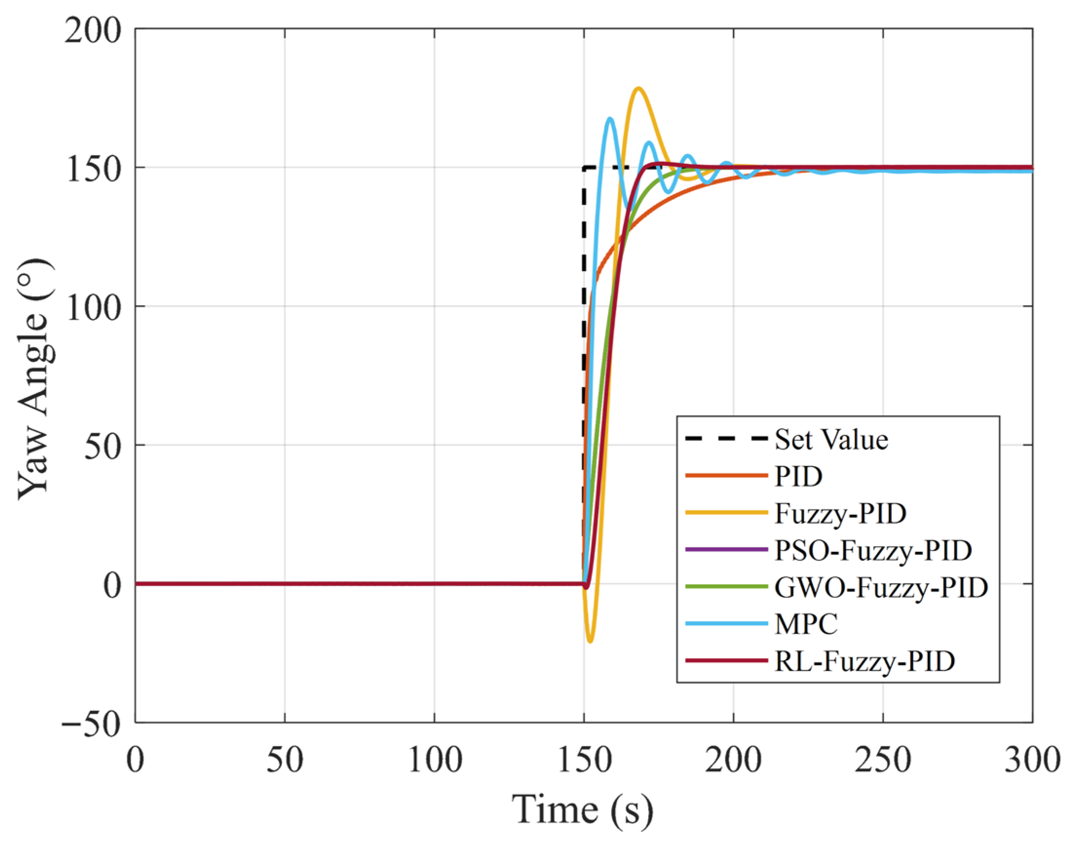
The step-response characteristics of the different yaw control schemes are illustrated in Figure 8. As can be observed, the proposed RL-based fuzzy PID controller exhibits faster convergence, reduced overshoot, and smoother yaw adjustment than the other controllers. These results indicate superior transient performance and actuation efficiency under deterministic conditions, thereby justifying the selection of the RL-Fuzzy-PID scheme as the reference controller for the subsequent turbulent-inflow evaluations.

Under IEC-compliant turbulent wind conditions, two representative inflow scenarios were considered in this study. Scenario 1 corresponds to an NTM case with a mean wind speed of 15 m/s and turbulence intensity class IEC-B. Scenario 2 corresponds to an ETM case with a mean wind speed of 18 m/s and turbulence intensity class IEC-A. For both scenarios, the turbulent wind fields were generated at a sampling frequency of 50 Hz with a horizontal grid size of 228 m × 228 m at each time step.

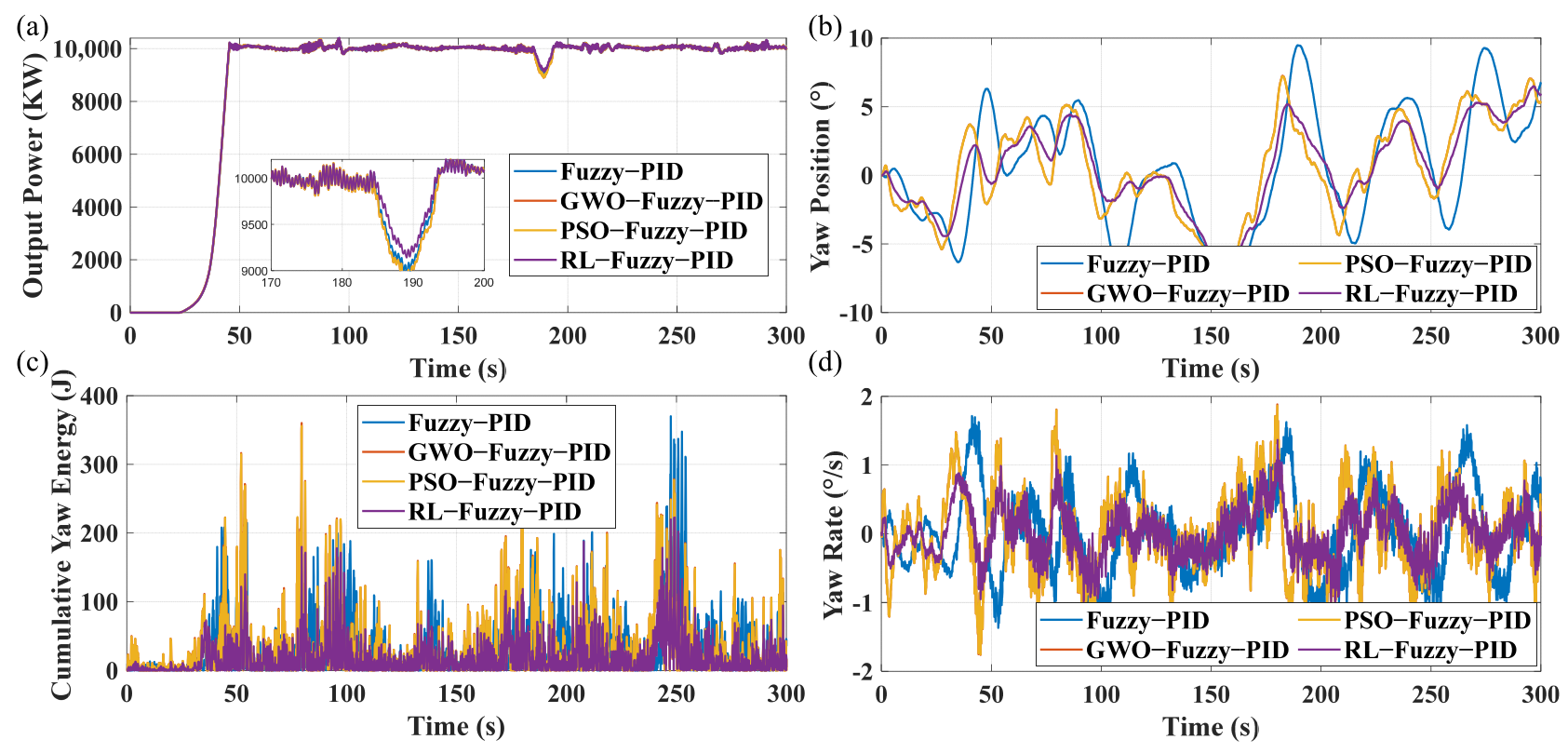
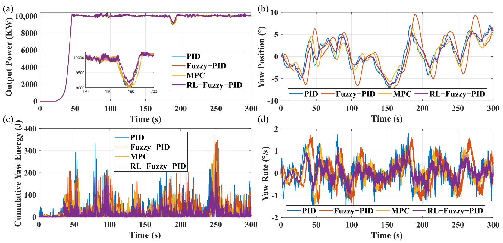
Figure 9 and Figure 10 present the responses of the different controllers in terms of output power, yaw position, cumulative yaw energy, and yaw rate under NTM conditions.

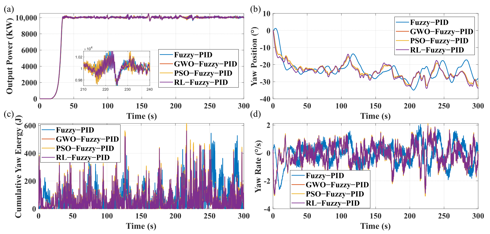
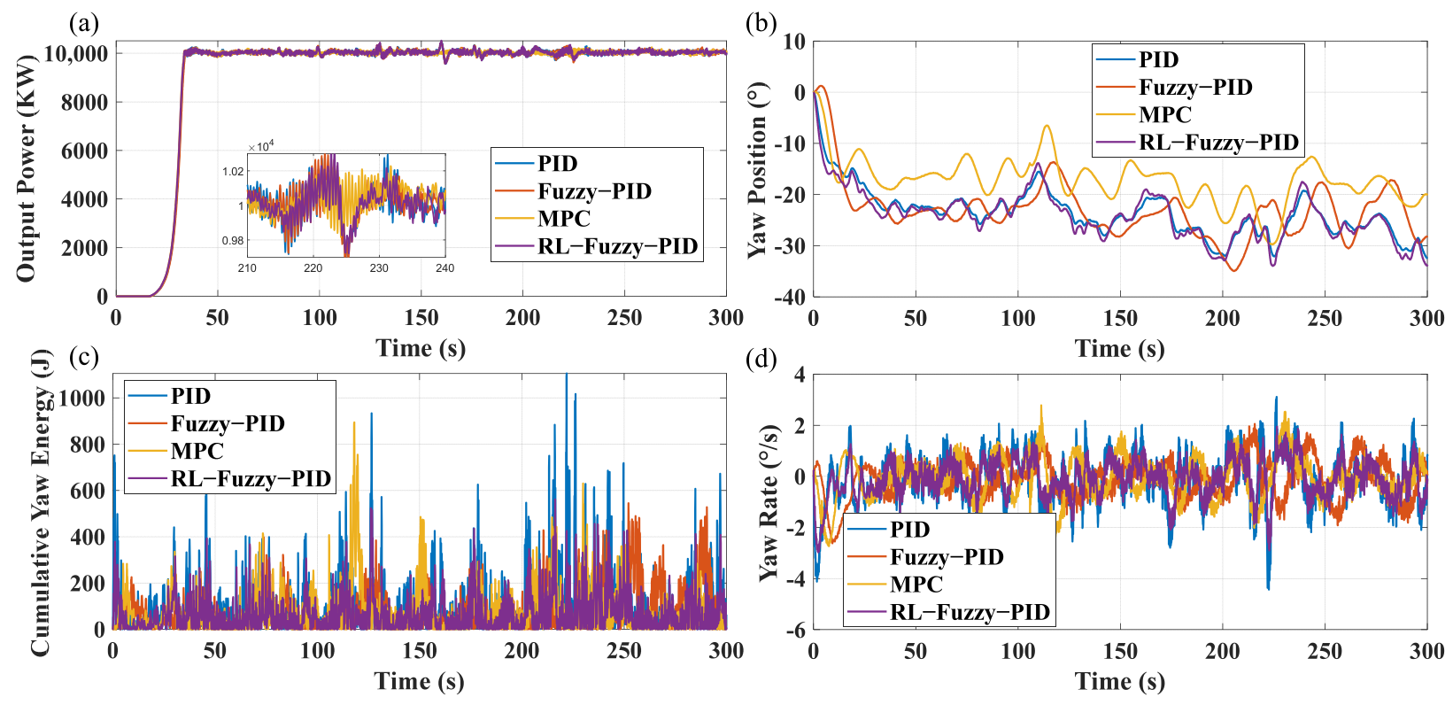
Figure 11 and Figure 12 present the corresponding comparative results under ETM conditions.

It should be noted that the PSO-Fuzzy-PID and GWO-Fuzzy-PID curves partially overlap in Figure 9 and Figure 11. This overlap is not caused by plotting error, but reflects the highly similar dynamic responses of the two optimization-based controllers under the tested turbulent wind conditions; this observation is further supported by the quantitative comparisons summarized in

Table 3. Performance comparison of different controllers under NTM.

Controller	Yaw Rate (RMS)	Cumulative Yaw Energy (KJ)	Output Power (STD)	Yaw Position (MAE)	Yaw Force (RMS)	Rotate (STD)	Transfer (STD)
PID	0.5429	8.8781	162.34	4.8592	6900.1	3.2815	6.1139
Fuzzy-PID	0.6010	9.3501	153.44	6.2690	6900.3	3.1851	6.1140
PSO	0.5648	9.3727	163.76	4.8203	6900.2	3.2825	6.1140
GWO	0.5673	9.4322	163.87	4.8187	6900.2	3.2823	6.1139
MPC	0.4578	6.8294	161.65	5.3577	6877.5	2.8631	5.6780
RL	0.3616	5.5110	133.05	5.2422	6900.1	3.2611	6.1137

and

Table 4. Performance comparison of different controllers under ETM.

Controller	Yaw Rate (RMS)	Cumulative Yaw Energy (KJ)	Output Power (STD)	Yaw Position (MAE)	Yaw Force (RMS)	Rotate (STD)	Transfer (STD)
PID	0.9818	28.944	91.937	6.8237	6820.0	2.9624	4.6695
Fuzzy-PID	0.7602	20.895	91.959	8.0316	6818.8	2.9016	4.7043
PSO	0.7643	20.619	91.783	6.7855	6819.9	2.9642	4.6690
GWO	0.7534	20.266	91.541	6.7980	6819.9	2.9635	4.6691
MPC	0.8164	20.732	66.396	9.2471	6793.8	2.5635	4.5364
RL	0.7303	19.515	91.144	6.5678	6819.9	2.9951	4.6637

.

The control performance is quantitatively evaluated using the root mean square (RMS), standard deviation (STD), and mean absolute error (MAE) indices.

$$RMS=\sqrt{{\displaystyle \frac{1}{N}}{\displaystyle \sum _{k=1}^N{x}^2(k)}}$$

(39)

$$STD=\sqrt{{\displaystyle \frac{1}{N}}{\displaystyle \sum _{k=1}^N{(x(k)-\overline{x})}^2}}$$

(40)

$$MAE={\displaystyle \frac{1}{N}}{\displaystyle \sum _{k=1}^N\left.\left|x(k)-x_{ref}(k)\right.\right|}$$

(41)

In addition to RMS, STD, and MAE, yaw-actuation energy consumption is quantified by integrating the absolute instantaneous yaw power over the simulation horizon:

$$E_{yaw}={\displaystyle {\int }_0^T\left|P_{yaw}\left(t\right)\right|}dt$$

(42)

where $P_{yaw}\left(t\right)$ denotes the instantaneous yaw power and $T$ is the evaluation duration. In the numerical implementation, this quantity is approximated in discrete form as ${\sum }_k\mid P_{yaw}\left(t_k\right)\mid \mathsf{\Delta }t$.

For force-, rotation-, and transmission-related variables, the three-dimensional discrete components are first combined into an equivalent resultant magnitude using the Euclidean norm. The corresponding RMS or STD values are then evaluated from the resultant signals over the entire simulation horizon.

$$x(k)=\sqrt{x_x^2(k)+x_y^2(k)+x_z^2(k)}$$

(43)

Table 3 and Table 4 summarize the quantitative performance of different yaw controllers under both NTM and ETM conditions, respectively.

Under NTM conditions, compared with the conventional PID, Fuzzy-PID, PSO-optimized Fuzzy-PID, GWO-optimized Fuzzy-PID, and MPC controllers, the proposed RL-based Fuzzy-PID reduces yaw-rate RMS by 33.4%, 39.8%, 36.0%, 36.2%, and 21.0%, respectively, while decreasing total yaw-energy consumption by 38.0%, 41.1%, 41.2%, 41.6%, and 19.3%. In addition, the yaw-position MAE is reduced by 8.0% relative to PID, indicating improved yaw alignment together with reduced actuation activity.

Under ETM conditions, compared with PID, Fuzzy-PID, PSO-optimized Fuzzy-PID, GWO-optimized Fuzzy-PID, and MPC, the proposed method reduces yaw-rate RMS by 25.6%, 3.9%, 4.4%, 3.1%, and 10.5%, respectively, while lowering total yaw-energy consumption by 32.6%, 6.6%, 5.4%, 3.7%, and 5.9%. In addition, a 28.9% reduction in yaw-position MAE is achieved relative to MPC, demonstrating improved yaw alignment accuracy and the effective suppression of unnecessary actuation under severe wind-direction fluctuations.

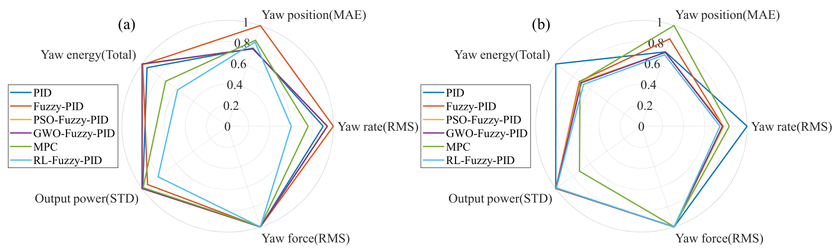
All performance indicators follow a “smaller-is-better” criterion. After normalization, a radar chart is used to provide an overall comparison of the different yaw control strategies, as shown in Figure 13. The results indicate that the RL-based controller attains relatively smaller normalized values for most indices, suggesting a more favorable trade-off among yaw accuracy, actuation effort, and power-related performance.

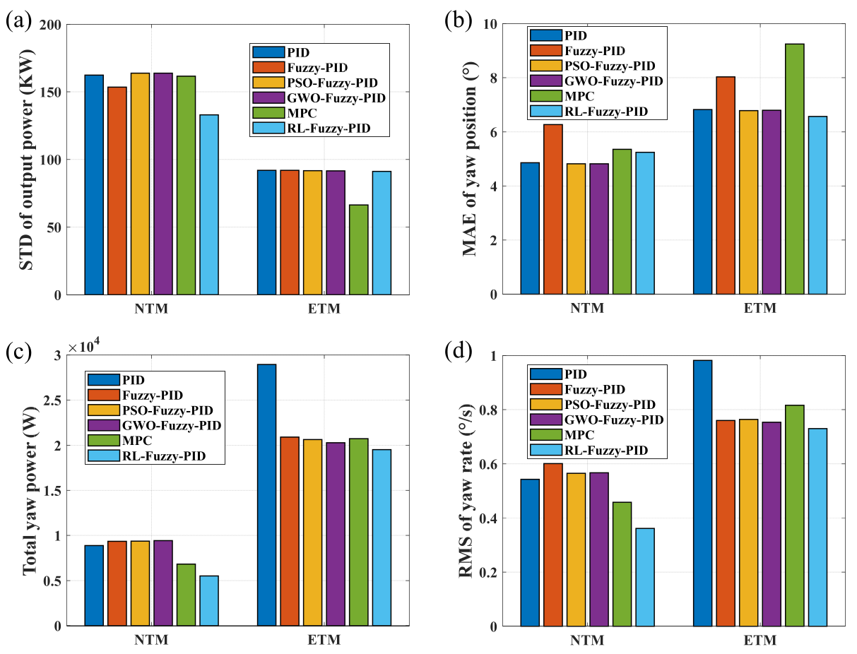
Figure 14 further illustrates the quantitative comparison of the different yaw control strategies under NTM and ETM conditions.

To more directly quantify the ability of the proposed RL-Fuzzy-PID controller to suppress unnecessary yaw activity, additional event-level yaw-motion statistics were introduced. To exclude the startup transient, all statistics were evaluated over the interval from 50 s to the end of each simulation. First, the yaw-rate signal $\dot{\psi }(t)$ was smoothed using a moving-average window of 0.5 s. Based on the smoothed signal, a yaw-motion state variable $d\left(t\right)$ was defined as follows:

$$d(t)=\left\{\begin{array}{c}+1,\\ -1,\\ 0,\end{array}\right.\begin{array}{c}{\dot{\psi }}_s(t)\ge {\omega }_{th}\\ {\dot{\psi }}_s(t)\le {\omega }_{th}\\ \left|{\dot{\psi }}_s(t)\right|<{\omega }_{th}\end{array}$$

(44)

where ${\dot{\psi }}_s(t)$ is the smoothed yaw rate and ${\omega }_{\mathrm{t}\mathrm{h}}$ is the yaw-rate threshold. A yaw-motion event was then defined as a sign-consistent nonzero segment of $d\left(t\right)$, after merging short zero gaps and removing segments with insufficient duration or amplitude.

Based on the detected yaw-motion events, the following indicators were calculated:

The yaw action count $N_{\mathrm{a}\mathrm{c}\mathrm{t}}$ is defined as the total number of detected yaw-motion events:

The direction-reversal count is defined as the number of sign changes between two consecutive yaw-motion events:

$$N_{rev}={\displaystyle \sum _{k=1}^{N_{act}-1}I\left(s_{k+1}\ne s_k\right)}$$

(45)

where $s_k\in \{+1,-1\}$ denotes the direction sign of the $k$-th yaw-motion event.

The cumulative yaw travel is defined as the total absolute yaw displacement over all detected yaw-motion events:

$$D_{yaw}={\displaystyle \sum _{k=1}^{N_{act}}{\displaystyle {\int }_{t_{s,k}}^{e,k}\left|\dot{\psi }(t)\right|}}dt$$

(46)

where $t_{s,k}$ and $t_{e,k}$ are the start and end times of the $k$-th yaw-motion event.

For the $k$-th yaw-motion event, the event amplitude is defined as:

$$A_k=\left|\psi (t_{e,k})-\psi (t_{s,k})\right|$$

(47)

where $\psi \left(t\right)$ is the yaw position.

The mean action amplitude is then calculated as follows:

$${\overline{A}}_{yaw}={\displaystyle \frac{1}{N_{act}}}{\displaystyle \sum _{k=1}^{N_{act}}{A}_k}$$

(48)

The resulting statistics under NTM and ETM conditions are summarized in

Table 5. Event-level yaw-motion statistics under NTM condition.

Controller	Yaw Action Count	Direction Reversal Count	Cumulative Yaw Travel (°)	Mean Action Amplitude (°)
PID	35	23	100.20	2.8162
Fuzzy-PID	17	13	120.72	7.0496
PSO	40	25	104.86	2.5814
GWO	40	25	105.34	2.5931
MPC	23	20	86.285	3.6977
RL	23	15	67.039	2.8490

and

Table 6. Event-level yaw-motion statistics under ETM condition.

Controller	Yaw Action Count	Direction Reversal Count	Cumulative Yaw Travel (°)	Mean Action Amplitude (°)
PID	46	30	127.23	2.6471
Fuzzy-PID	46	36	176.92	3.6109
PSO	44	34	137.78	3.0582
GWO	43	34	135.55	3.0782
MPC	24	20	148.19	6.0875
RL	26	18	135.29	5.1267

.

The event-level yaw-motion statistics in Table 5 and Table 6 provide direct quantitative evidence of the yaw-actuation behavior of the compared controllers. Under NTM conditions, RL-Fuzzy-PID exhibits the most balanced yaw-motion pattern, characterized by the lowest direction-reversal count and the lowest cumulative yaw travel among all controllers. Compared with PID, Fuzzy-PID, PSO-Fuzzy-PID, GWO-Fuzzy-PID, and MPC, its cumulative yaw travel is reduced by 33.1%, 44.5%, 36.1%, 36.4%, and 22.3%, respectively. Although Fuzzy-PID yields fewer yaw actions, its much larger cumulative yaw travel and mean action amplitude indicate a heavier actuation burden. Under ETM conditions, RL-Fuzzy-PID still maintains a relatively low yaw-action count, the lowest direction-reversal count, and a comparatively low cumulative yaw travel, with reductions of 23.5%, 1.8%, 0.2%, and 8.7% relative to Fuzzy-PID, PSO-Fuzzy-PID, GWO-Fuzzy-PID, and MPC, respectively. These results indicate that RL-Fuzzy-PID suppresses unnecessary reversal-dominated yaw activity under NTM and preserves a more organized correction pattern under ETM.

3.3. Robustness and Sensitivity Evaluation

3.3.1. Sensitivity to Communication Delay and Packet Loss

To further evaluate the applicability of the proposed distributed soft-real-time co-simulation framework under impaired communication conditions, a sensitivity analysis was conducted under the ETM condition by introducing fixed delay and packet loss into the wind-direction measurement channel. To exclude startup transients, all indices were evaluated over a common post-startup window from 50 s to the end of the simulation.

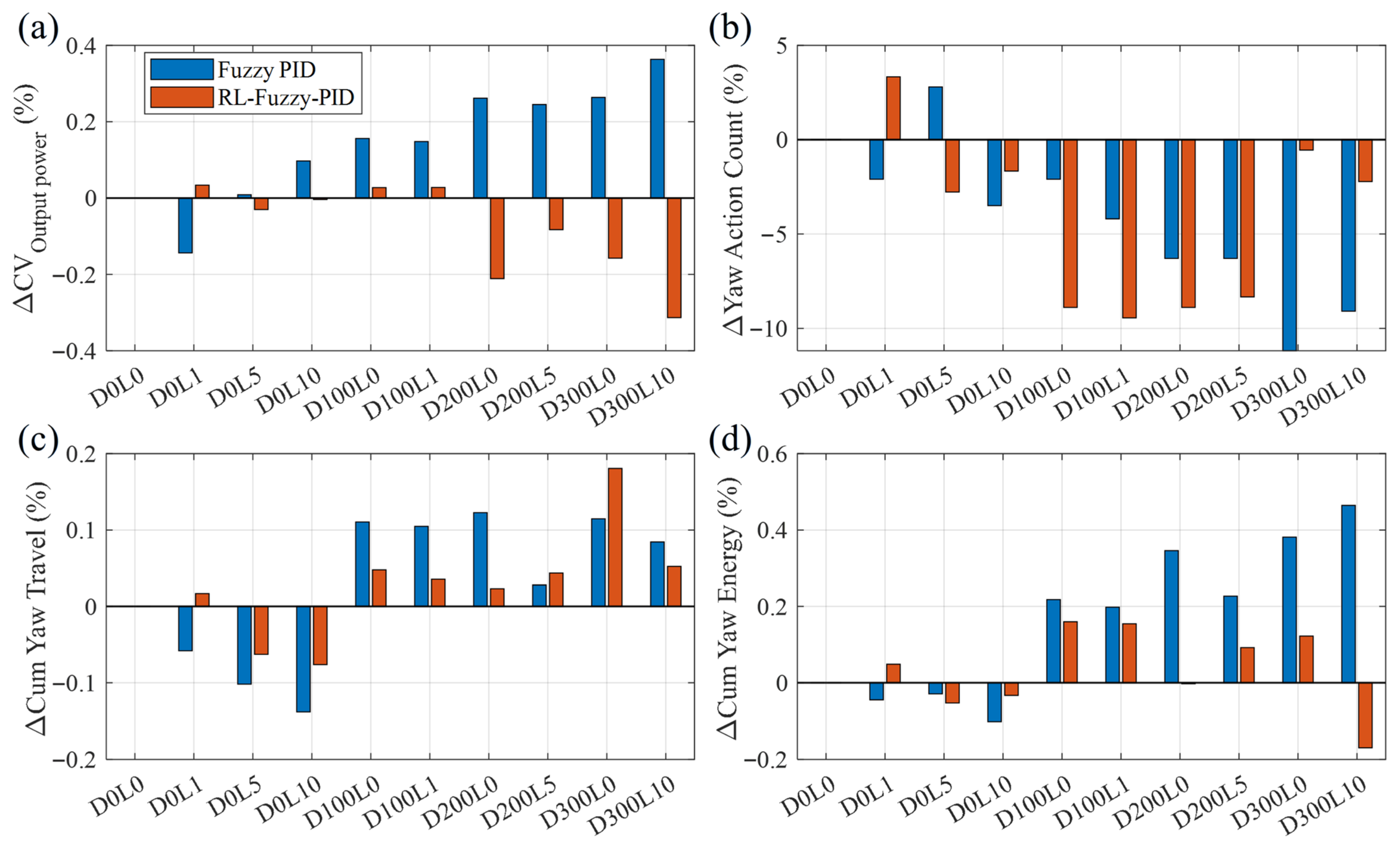
The communication conditions are denoted in the form $D\cdot L$, where $D$ represents the fixed delay in milliseconds and $L$ represents the packet-loss rate in percent. Accordingly, D0L0 denotes the no-impairment baseline, D0L10 denotes the case with 10% packet loss only, D100L0 denotes the case with 100 ms delay only, and D300L10 denotes the combined severe case with 300 ms delay and 10% packet loss. These cases were selected to represent the baseline condition, single-factor degradation, and a representative severe communication-impairment scenario.

Representative results are summarized in

Table 7. Representative post-startup performance metrics under communication delay and packet-loss conditions.

Case	Controller	Cumulative Yaw Energy (KJ)	Cumulative Yaw Travel (°)	Output Power (CV)	Yaw Action Count
D0L0	Fuzzy-PID	20.895	176.92	0.8435	46
	RL-Fuzzy-PID	19.515	135.29	0.8173	26
D0L10	Fuzzy-PID	20.780	175.84	0.8435	44
	RL-Fuzzy-PID	19.320	135.17	0.8181	25
D100L0	Fuzzy-PID	21.021	177.27	0.8437	45
	RL-Fuzzy-PID	19.686	135.37	0.8186	21
D300L10	Fuzzy-PID	21.552	177.23	0.8409	42
	RL-Fuzzy-PID	19.236	135.38	0.8203	24

. The output-power coefficient of variation, denoted as Output Power (CV), is calculated as follows:

$$OutputPowerCV={\displaystyle \frac{\sigma (P_{out})}{{\overline{P}}_{out}}}\times 100\%$$

(49)

where $\sigma \left(P_{\mathrm{o}\mathrm{u}\mathrm{t}}\right)$ and ${\overline{P}}_{\mathrm{o}\mathrm{u}\mathrm{t}}$ denote the standard deviation and mean value of output power, respectively, within the common evaluation window.

To further quantify the sensitivity of each controller to communication degradation, the relative changes in the key indices with respect to each controller’s own baseline case (D0L0) are shown in Figure 15. In this figure, the horizontal axis represents the communication-impairment cases, whereas the vertical axis represents the relative percentage change in each metric with respect to the corresponding no-impairment baseline. Accordingly, a positive value indicates an increase relative to the baseline, whereas a negative value indicates a decrease. This figure reflects the sensitivity of each controller to communication degradation rather than a direct comparison of their absolute performance levels.

As shown in Figure 15, the relative variations in the CV of output power, Cumulative yaw travel, and Cumulative yaw energy remained small across all tested cases, indicating that the overall closed-loop performance was only mildly affected by the introduced delay and packet loss. By contrast, Yaw action count exhibited the largest variation, suggesting that communication degradation affected yaw-actuation behavior more noticeably than power-related performance. Moreover, the RL-Fuzzy-PID controller generally showed smaller relative deviations from its own baseline in several representative cases, indicating better robustness to communication impairment in relative-performance terms.

Overall, these results show that the proposed framework can serve as a soft-real-time, network-aware co-simulation platform for controller evaluation under communication delay and packet loss. Within the tested impairment range, the closed-loop system remained stable, the average generated power was nearly unaffected, and the main impact of communication degradation was observed in yaw-actuation behavior rather than mean power-capture capability.

3.3.2. Sensitivity Analysis Under Corrupted Input Data

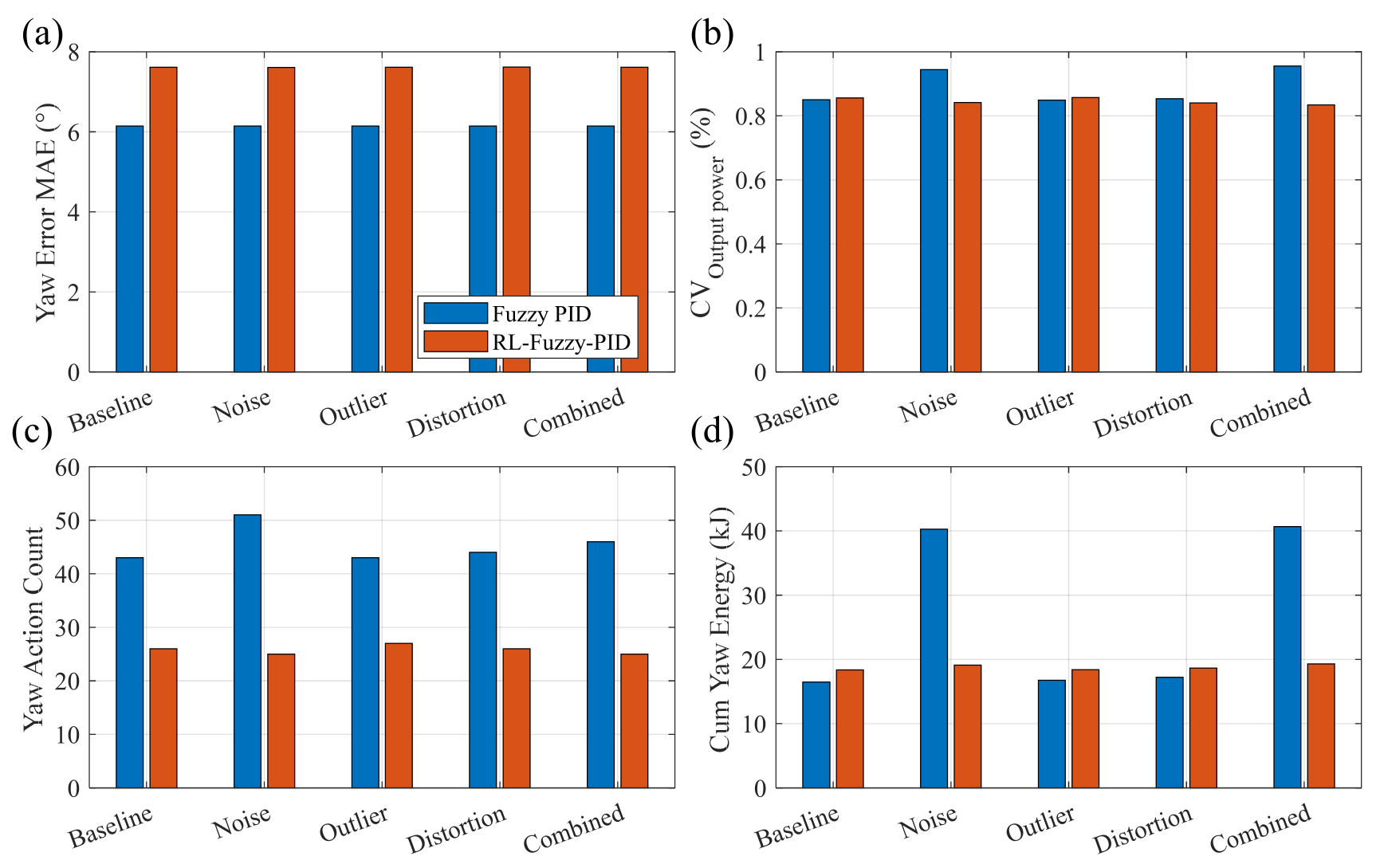
Additional robustness tests were conducted under the ETM condition by injecting corrupted signals into the controller-side wind-direction input. In addition to the baseline case (0), additive noise (N), impulsive outliers (O), signal distortion (D), and the combined case (C) were considered. To eliminate startup effects, all metrics were evaluated over the interval from 50 s to the end of the simulation. To provide a more intuitive comparison of the robustness trends under different input perturbations, the key performance metrics of the two controllers are further summarized in Figure 16. The corresponding numerical results are listed in

Table 8. Performance metrics of Fuzzy PID and RL-Fuzzy-PID under corrupted input data.

Case	Controller	Cumulative Yaw Energy (KJ)	Output Power (CV)	Yaw Error (MAE)	Cumulative Yaw Travel (°)	Yaw Action Count
Baseline	Fuzzy-PID	16.489	0.8500	6.1445	176.92	43
	RL-Fuzzy-PID	18.384	0.8561	7.6142	135.29	26
Noise	Fuzzy-PID	40.277	0.9443	6.1459	233.02	51
	RL-Fuzzy-PID	19.105	0.8415	6.6060	144.64	25
Outlier	Fuzzy-PID	16.754	0.8490	6.1456	138.18	43
	RL-Fuzzy-PID	18.404	0.8573	7.6130	140.43	27
Distortion	Fuzzy-PID	17.218	0.8535	6.1427	140.93	44
	RL-Fuzzy-PID	18.641	0.8404	7.6186	141.83	26
Combined	Fuzzy-PID	40.683	0.9552	6.1438	234.96	46
	RL-Fuzzy-PID	19.300	0.8342	7.6219	145.84	25

for detailed quantitative comparison.

Table 8 summarizes the corresponding results. Both controllers remained stable under all tested perturbation conditions, and the yaw-tracking error varied only slightly. However, their degradation patterns differed markedly in actuation-related metrics. For the conventional Fuzzy-PID controller, the noise case increased the power-fluctuation coefficient, yaw-action count, cumulative yaw displacement, and cumulative yaw energy by 11.1%, 79.3%, 70.3%, and 144.3%, respectively, relative to its own baseline. Under the combined case, the corresponding increases reached 12.4%, 85.4%, 71.7%, and 146.7%

In contrast, the proposed RL-Fuzzy-PID controller showed much smaller degradation under the same perturbation conditions. Relative to its own baseline, the noise case changed these four metrics by −1.7%, +30.1%, +3.0%, and +3.9%, respectively, whereas the combined case yielded −2.6%, +19.2%, +3.9%, and +5.0%. Under the outlier and distortion cases, both controllers showed only limited degradation. Overall, the robustness benefit of the proposed RL-based tuning is mainly reflected in mitigating excessive yaw activity and energy deterioration under persistent input corruption.

3.3.3. Sensitivity Analysis of Learning Rate, Reward Architecture, and Initialization

To assess the algorithm-level robustness of the proposed RL-assisted offline tuner, additional sensitivity analyses were performed in the reduced-order training environment derived from the yaw-system state-space model. In this fast-screening setting, a pulse-type yaw-reference input was adopted to isolate the influence of key tuning-related factors, whereas the higher-fidelity turbulent-inflow validation of the final controller was retained in the main simulation section. In this setting, the reduced-order screening objective was constructed from normalized tracking-related and actuation-related terms, so that the optimization process could be compared under different hyperparameter choices in a unified manner.

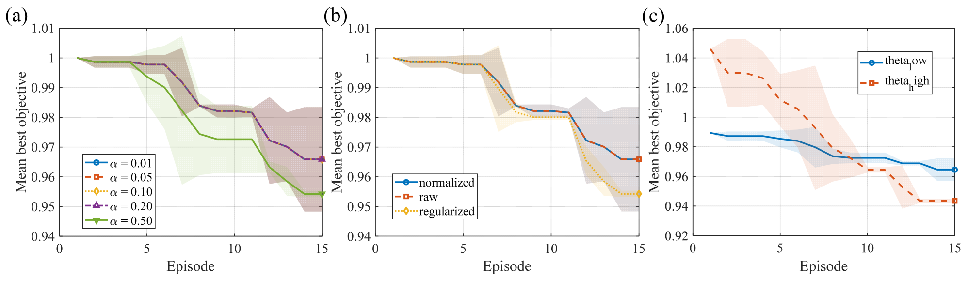
First, learning-rate sensitivity was examined using $\alpha =0.01$, 0.05, 0.10, 0.20, and 0.50, each tested under two random seeds. As shown in Figure 17a, the optimization trajectories remain highly similar across most of the tested practical learning-rate range, and the final best-objective values also remain close to one another. Only the largest tested value, $\alpha =0.50$, shows a slightly more noticeable deviation for one seed. These results indicate that the proposed offline RL tuner exhibits limited sensitivity to the learning-rate choice in terms of the final tuning outcome, whereas the learning rate mainly affects the convergence path and the degree of path-dependent variation.

Second, reward-architecture sensitivity was evaluated using three reward formulations: a normalized fitness-improvement reward, a raw fitness-improvement reward, and a regularized reward with an additional parameter-update penalty. Figure 17b shows that the normalized and raw rewards produce nearly overlapping optimization trajectories in the present screening environment, suggesting that the search behavior is mainly governed by the direction of fitness improvement rather than the exact reward scaling. By contrast, the regularized reward leads to a slightly different convergence path and a different final parameter combination, indicating that the reward architecture mainly affects the detailed trade-off among performance terms rather than the overall tuning conclusion.

Third, initialization sensitivity was examined using two distinct starting points, namely a lower-biased initial vector ${\theta }_{\mathrm{low}}$ and a higher-biased initial vector ${\theta }_{\mathrm{high}}$, under a fixed learning-rate setting. As shown in Figure 17c, initialization exerts a more visible influence on the optimization trajectory than the learning-rate and reward variations. The lower-biased initialization tends to converge toward a solution with lower tracking-related indices, whereas the higher-biased initialization tends to yield lower actuation-related terms at the cost of slightly worse tracking performance. Thus, initialization mainly influences which local performance trade-off is selected, while both tested initializations still converge to stable tuned solutions.

Overall, these results show that the proposed RL-assisted tuning framework is reasonably stable in the reduced-order offline tuning environment. The main conclusion does not depend on a single isolated choice of learning rate, reward formulation, or initialization, although moderate differences may still appear in convergence behavior and detailed parameter evolution.

3.4. Online Execution-Time Profiling on the Controller-Side Processor

To evaluate online computational efficiency on the target controller-side processor, an additional controller-only replay benchmark was conducted. Two prerecorded input signals, namely nacelle yaw position and hub-height wind direction, were extracted from a representative co-simulation run and replayed to each controller under the same software and hardware environment. In this benchmark, only controller-side computation was timed, whereas OpenFAST (version 4.0.0) plant integration and inter-process communication overhead were excluded. For the proposed RL-assisted method, the reported execution time refers only to the online execution of the final tuned Fuzzy-PID controller, while the offline Q-learning stage is excluded from the per-step timing comparison. Each benchmark was repeated five times, and the average, maximum, and 95th-percentile per-step execution times were recorded.

Table 9. Online execution time per control step measured on the controller-side processor.

Controller	Average Run Time (s)	Average Step Time (ms)	Max Step Time (ms)	95th Percentile (ms)
PID	1.071	0.071	0.089	0.089
Fuzzy-PID	60.994	4.066	4.410	4.410
RL-Fuzzy-PID	56.734	3.782	3.946	3.946

summarizes the controller-side execution times obtained from the replay benchmark. As expected, the classical PID controller exhibits the lowest computational burden, with an average execution time of 0.071 ms per step. The conventional Fuzzy-PID controller requires a higher computational cost, reaching an average of 4.066 ms per step. The proposed RL-Fuzzy-PID controller shows a similar online computational level, with an average execution time of 3.782 ms per step and a maximum value of 3.946 ms.

These results show that the proposed method is not faster than classical PID in raw online computational speed. However, its online execution cost remains close to that of conventional Fuzzy-PID, since RL is used only for offline parameter tuning and does not participate in per-step online learning. Under the present replay benchmark, the effective input update interval was 0.02 s, and the measured execution times of both Fuzzy-PID and RL-Fuzzy-PID remained below this interval, indicating that the proposed controller satisfies the timing requirement of the current co-simulation configuration.

In addition, the online computational burden of the benchmark MPC was profiled under the final controller settings. With a controller update period of 20 ms, the measured average, 95th-percentile, and maximum optimization times were 0.545 ms, 0.838 ms, and 3.343 ms, respectively. Since the worst-case optimization time remained well below the update period, the benchmark MPC could complete online optimization within the timing requirement of the present distributed soft-real-time co-simulation framework.

4. Discussion

The results indicate that the proposed RL-assisted Fuzzy-PID controller achieves a more favorable compromise between yaw-tracking performance and actuation economy than the benchmark controllers, although the improvement is not uniform across all indices. Under NTM conditions, the RL-based scheme attains the lowest yaw-rate RMS, the lowest total yaw-energy consumption, and the smallest output-power fluctuation among the compared methods. This indicates that the main contribution of RL is not merely faster response, but a more selective use of yaw actuation under continuously varying wind conditions. In other words, the controller tends to avoid excessive corrective motion when the instantaneous yaw error does not justify aggressive adjustment.

Under ETM conditions, the performance differences among the advanced controllers become smaller, which is reasonable because all controllers operate closer to the physical limits of the yaw system under intensified wind-direction fluctuations. Even under this more severe condition, the RL-based controller still yields the lowest yaw-rate RMS, the lowest total yaw-energy consumption, and the smallest yaw-position MAE among the compared methods. This suggests that the proposed method remains effective in preserving control stability while limiting unnecessary actuator usage under high-disturbance inflow.

Another notable observation is that the advantage of the proposed controller is more pronounced in actuation-related indices than in structural-response-related indices. The substantial reductions in yaw-rate RMS and yaw energy, together with the relatively limited differences in yaw force, rotation, and transmission indicators, suggest that the controller primarily improves yaw-control efficiency rather than fundamentally changing the aeroelastic load path of the turbine. This is physically reasonable because those structural responses are jointly determined by turbulence intensity, aeroelastic coupling, drivetrain dynamics, and structural flexibility, and therefore cannot be reshaped by yaw control alone.

The event-level yaw-motion statistics further clarify the mechanism behind the favorable actuation-related performance of RL-Fuzzy-PID. The key advantage is not simply faster correction, but a more appropriate redistribution of yaw actions between responsiveness and actuator burden. In this sense, the RL-based tuning process does not merely adjust gain values; it reshapes the overall yaw-motion pattern.

Under NTM conditions, RL-Fuzzy-PID produces fewer yaw actions than PID and the PSO-/GWO-based controllers, while simultaneously achieving the lowest direction-reversal count and the lowest cumulative yaw travel. This indicates that the controller is less likely to respond to short-lived wind-direction fluctuations with repeated corrective commands. The comparison with Fuzzy-PID is particularly informative: although Fuzzy-PID yields the smallest action count, it also exhibits the largest cumulative yaw travel and a much larger mean action amplitude. Therefore, the benefit of RL-based tuning lies not in minimizing event count alone, but in optimizing the overall structure of yaw motion.

Under ETM conditions, corrective yaw actions become harder to avoid because the disturbance intensity is stronger and more persistent. In this regime, the practical advantage of RL-Fuzzy-PID is not that it minimizes all motion-related indices simultaneously, but that it preserves a more organized yaw-motion pattern. By maintaining the lowest direction-reversal count together with comparatively low cumulative yaw travel, while allowing a somewhat larger mean action amplitude, the controller appears to favor fewer repetitive oscillatory corrections and more decisive responses to large disturbances. Thus, under severe turbulence, the main benefit of RL-Fuzzy-PID lies less in enforcing minimum motion count at all costs and more in reducing reversal-dominated actuator burden.

From an engineering perspective, these findings are important because offshore yaw systems are sensitive not only to the total amount of nacelle rotation, but also to repeated reversal behavior and fragmented control actions. Frequent reversals and redundant small corrections can accelerate wear in motors, gears, and bearings without yielding proportional aerodynamic benefit. Accordingly, the practical value of RL-Fuzzy-PID lies not only in improved control performance, but also in the mitigation of long-term actuation burden.

The comparison with PSO- and GWO-based Fuzzy-PID controllers is also informative because all three methods are used here as offline tuning strategies rather than online end-to-end controllers. However, unlike conventional population-based metaheuristic search, the RL-assisted scheme updates parameters through a tabular sequential learning process in the discretized parameter space and retains the best-performing parameter set identified during training. For the bounded five-parameter tuning problem considered in this study, tabular Q-learning provides a transparent and computationally tractable learning mechanism. The value of RL in this work therefore lies not in deep policy approximation, but in providing a structured simulation-guided mechanism for identifying a better compromise between response quality and actuator burden.

The benchmark MPC should be interpreted in the context of its reduced-order delayed internal prediction model, whereas the controlled plant in co-simulation is the full nonlinear OpenFAST-based yaw system under stochastic turbulent excitation. Consequently, model mismatch is inherently present in the MPC benchmark. The simplified predictor was adopted to maintain a practically implementable and computationally tractable receding-horizon controller within the present framework, rather than to intentionally weaken the model-based approach. As disturbance intensity and nonlinear coupling increase, the discrepancy between the predictor and the actual plant becomes more influential, which can weaken prediction accuracy and reduce the optimization effectiveness of MPC. This likely explains why MPC remains acceptable under milder conditions but becomes less competitive under severe turbulence.

The distributed co-simulation environment further strengthens the practical relevance of the present study. The controller is not evaluated in an idealized standalone simulation, but in a framework that explicitly includes asynchronous sampling, inter-process communication, and startup synchronization. Therefore, the reported results are more representative of network-aware implementation conditions than those obtained from purely offline controller-tuning studies. This is particularly relevant for yaw-control applications, in which communication delay, signal exchange, and platform coordination can noticeably influence closed-loop behavior.

Several limitations should nevertheless be acknowledged. First, the present validation is based on a PC-based soft real-time co-simulation platform rather than hardware-in-the-loop testing or field deployment, so the effects of industrial communication jitter, embedded computation delay, and sensor quantization have not yet been fully quantified. Second, the yaw actuator is represented by a simplified dynamic model, and nonlinear effects such as backlash, stiction, torque saturation, and thermal constraints are not explicitly included. Third, the RL tuning protocol is scenario-specific: The tabular Q-learning procedure was conducted separately for NTM and ETM, and each condition was evaluated using its own tuned parameter set. Accordingly, the present results demonstrate the effectiveness of scenario-specific offline tuning, but do not yet constitute a strict cross-condition generalization study in which one parameter set learned under a given wind regime is directly applied to unseen turbulence conditions. Future work should therefore consider hard real-time implementation, richer actuator and sensor uncertainty modeling, and broader transfer evaluation across unseen wind regimes and wake-coupled operating conditions.

5. Conclusions

This paper presents an RL-assisted Fuzzy-PID yaw control framework for large-scale offshore wind turbines operating under nonlinear dynamics and stochastic wind disturbances. In the proposed method, tabular Q-learning is employed as a low-dimensional offline tuning strategy to optimize the quantization and scaling parameters of the Fuzzy-PID controller in a discretized five-dimensional parameter space. The resulting controller is validated through a high-fidelity distributed co-simulation framework integrating IEC-compliant TurbSim wind fields, the OpenFAST aero-hydro-servo-elastic model, and a Simulink-based yaw control system under soft real-time communication constraints.

Simulation results under step-change, normal-turbulence, and extreme-turbulence conditions show that the proposed RL-assisted Fuzzy-PID controller provides a more favorable trade-off between yaw-tracking quality and actuator usage than the benchmark controllers. In particular, the proposed method achieves clear reductions in yaw-rate RMS and yaw-energy consumption, while also suppressing unnecessary yaw motion and improving output-power stability under stochastic wind conditions. These findings suggest that the practical value of the proposed strategy lies not in introducing a fundamentally new control theory, but in providing a simulation-guided tuning framework that improves the compromise between yaw-alignment performance and actuation economy for large offshore wind turbines.

Nevertheless, the present study is limited to a PC-based soft real-time co-simulation environment, and the yaw-actuator model remains simplified. Future work will therefore focus on hard real-time implementation, richer actuator and sensor uncertainty modeling, and the extension of the proposed framework to wind-farm-level cooperative yaw control under wake-interaction-aware operating conditions.

References

1. Elkodama, A.; Ismaiel, A.; Abdellatif, A.; Shaaban, S.; Yoshida, S.; Rushdi, M.A. Control Methods for Horizontal Axis Wind Turbines (HAWT): State-of-the-Art Review. Energies 2023, 16, 6394. [Google Scholar] [CrossRef] [Scilit]
2. Choi, H.-S.; Kim, J.-G.; Cho, J.-H.; Nam, Y.-S. Active Yaw Control of MW class Wind Turbine. In Proceedings of the International Conference on Control, Automation and Systems (ICCAS 2010), Goyang-si, Republic of Korea, 27–30 October 2010; IEEE: Piscataway, NJ, USA, 2010; pp. 1075–1078. [Google Scholar]
3. Elkodama, A.; Abdellatif, A.; Shaaban, S.; Rushdi, M.A.; Yoshida, S.; Ismaiel, A. Investigation into the Yaw Control of a Twin-Rotor 10 MW Wind Turbine. Appl. Sci. 2024, 14, 9810. [Google Scholar] [CrossRef] [Scilit]
4. Hu, Y.; Luo, P.; Yao, W.; Zhou, L.; Shi, P.; Yang, W.; Han, H. Power increase and lifespan extension control strategy of wind turbine yaw system based on power loss. Sustain. Energy Technol. Assess. 2025, 74, 104172. [Google Scholar] [CrossRef] [Scilit]
5. Liu, Y.; Liu, S.; Zhang, L.; Cao, F.; Wang, L. Optimization of the Yaw Control Error of Wind Turbine. Front. Energy Res. 2021, 9, 626681. [Google Scholar] [CrossRef] [Scilit]
6. Zhu, J.; Zhu, J.; Chen, G.; Xu, C.; Meng, X.; Hu, H. Yaw System Control Strategy for Wind Turbines Based on Turbulence Intensity and Operating Modes. In Proceedings of the 2024 6th International Conference on Electrical Engineering and Control Technologies (CEECT), Shenzhen, China, 20–22 December 2024; pp. 76–81. [Google Scholar]
7. Zhao, H.; Zhou, L.; Zhang, S.; Liang, Y. XE112-2000 Wind Turbine Yaw Strategy with Adaptive Yaw Speed Using DEL Look-Up Table. IEEE Access 2021, 9, 125724–125738. [Google Scholar] [CrossRef] [Scilit]
8. Theodoropoulos, S.; Kandris, D.; Samarakou, M.; Koulouras, G. Fuzzy regulator design for wind turbine yaw control. Sci. World J. 2014, 2014, 516394. [Google Scholar] [CrossRef] [Scilit]
9. Torabi, A.; Tarsaii, E.; Mousavi Mashhadi, S.K. Fuzzy Controller Used in Yaw System of Wind Turbine Noisy. J. Math. Comput. Sci. 2014, 8, 105–112. [Google Scholar] [CrossRef] [Scilit]
10. Song, D.; Fan, X.; Yang, J.; Liu, A.; Chen, S.; Joo, Y.H. Power extraction efficiency optimization of horizontal-axis wind turbines through optimizing control parameters of yaw control systems using an intelligent method. Appl. Energy 2018, 224, 267–279. [Google Scholar] [CrossRef] [Scilit]
11. Hure, N.; Turnar, R.; Vasak, M.; Bencic, G. Optimal Wind Turbine Yaw Control Supported with Very Short-term Wind Predictions. In Proceedings of the IEEE International Conference on Industrial Technology (ICIT), Seville, Spain, 17–19 March 2015; IEEE: Piscataway, NJ, USA, 2015; pp. 385–391. [Google Scholar]
12. Chen, W.; Liu, H.; Lin, Y.; Li, W.; Sun, Y.; Zhang, D. LSTM-NN Yaw Control of Wind Turbines Based on Upstream Wind Information. Energies 2020, 13, 1482. [Google Scholar] [CrossRef] [Scilit]
13. Bao, Y.; Yang, Q. A Data-Mining Compensation Approach for Yaw Misalignment on Wind Turbine. IEEE Trans. Ind. Inform. 2021, 17, 8154–8164. [Google Scholar] [CrossRef] [Scilit]
14. Bao, Y.; Yang, Q.; Li, S.; Miao, K.; Sun, Y. A Data-Driven Approach for Identification and Compensation of Wind Turbine Inherent Yaw Misalignment. In Proceedings of the 33rd Youth Academic Annual Conference of Chinese Association of Automation (YAC), Nanjing, China, 18–20 May 2018; IEEE: Piscataway, NJ, USA, 2018; pp. 961–966. [Google Scholar]
15. Saenz-Aguirre, A.; Zulueta, E.; Fernandez-Gamiz, U.; Lozano, J.; Lopez-Guede, J.M. Artificial Neural Network Based Reinforcement Learning for Wind Turbine Yaw Control. Energies 2019, 12, 436. [Google Scholar] [CrossRef] [Scilit]
16. Puech, A.; Read, J. An Improved Yaw Control Algorithm for Wind Turbines via Reinforcement Learning. In Proceedings of the European Conference on Machine Learning and Principles and Practice of Knowledge Discovery in Databases (ECML-PKDD), Grenoble, France, 19–23 September 2022; pp. 614–630. [Google Scholar]
17. Sadraddin, H.L.; Shao, X. Distributed real-time hybrid simulation method for dynamic response evaluation of floating wind turbines. Eng. Struct. 2024, 303, 117464. [Google Scholar] [CrossRef] [Scilit]
18. Qu, C.; Lin, Z.; Liu, J.; Yu, Y.; Tian, X.; Yuan, Z. Modeling and hardware-in-the-loop implementation of real-time aero-elastic-electrical co-simulation platform for PMSG wind turbine. Appl. Energy 2024, 359, 122777. [Google Scholar] [CrossRef] [Scilit]
19. Jonkman, J.; Buhl, M.L. FAST User’s Guide—Updated August 2005; National Renewable Energy Laboratory (NREL): Golden, CO, USA, 2005. [Google Scholar] [CrossRef] [Scilit]
20. IEC 61400-1:2019; Wind Energy Generation Systems—Part 1: Design Requirements. International Electrotechnical Commission: Geneva, Switzerland, 2019.
21. Bak, C.; Zahle, F.; Bitsche, R.; Kim, T.; Yde, A.; Henriksen, L.C.; Andersen, P.B.; Natarajan, A.; Hansen, M.H. Design and Performance of a 10 MW Wind Turbine; DTU Wind Energy Report-I-0092; Danmarks Tekniske Universitet: Kongens Lyngby, Denmark, 2013; Volume 124. [Google Scholar]
22. Lin, M.; Porté-Agel, F. Power Production and Blade Fatigue of a Wind Turbine Array Subjected to Active Yaw Control. Energies 2023, 16, 2542. [Google Scholar] [CrossRef] [Scilit]
23. Sadeghi, M.S.; Varzandian, S.; Barzegar, A. Optimization of Classical PID and Fuzzy PID Controllers of a Nonlinear Quarter Car Suspension System Using PSO Algorithm. In Proceedings of the 1st International eConference on Computer and Knowledge Engineering (ICCKE), Ferdowsi Univ Mashhad, Mashhad, Iran, 13–14 October 2011; IEEE: Piscataway, NJ, USA, 2011; pp. 172–176. [Google Scholar]
24. Li, X.; Zhang, S.; Zheng, F.; Wang, B. Fuzzy Neural Network PID Control of Quadrotor Unmanned Aerial Vehicle Based on PSO-GA Optimization. In Proceedings of the 11th International Conference on Modelling, Identification and Control (ICMIC), Tianjin, China, 13–15 July 2019; pp. 335–345. [Google Scholar]
25. Kang, H.B.; Zhang, Z.W.; Jin, L.; Zhang, C.; Li, X.H.; Zhu, J.H.; Yang, Z.Y. Design and Testing of an Electrically Driven Precision Soybean Seeder Based an OGWO-Fuzzy PID Control Strategy. Appl. Sci. 2025, 15, 9318. [Google Scholar] [CrossRef] [Scilit]
26. Rubert, T.; Perry, M.; Fusiek, G.; McAlorum, J.; Niewczas, P.; Brotherston, A.; McCallum, D. Field Demonstration of Real-Time Wind Turbine Foundation Strain Monitoring. Sensors 2018, 18, 97. [Google Scholar] [CrossRef] [Scilit]
27. Yadav, S.; Namrata, K.; Kumar, N.; Samadhiya, A. Fuzzy based load frequency control of power system incorporating nonlinearity. In 2022 4th International Conference on Energy, Power and Environment (ICEPE); IEEE: Piscataway, NJ, USA, 2022. [Google Scholar]
28. Liu, Y.Y.; As’arry, A.; Ahmed, H.; Hairuddin, A.A.; Hassan, M.K.; Zakaria, M.Z.; Yang, S. Online optimal tuning of fuzzy PID controller using grey wolf optimizer for quarter car semi-active suspension system. Adv. Mech. Eng. 2024, 16, 16878132231219620. [Google Scholar] [CrossRef] [Scilit]
29. Starke, G.M.; Meneveau, C.; King, J.R.; Gayme, D.F. A dynamic model of wind turbine yaw for active farm control. Wind Energy 2024, 27, 1302–1318. [Google Scholar] [CrossRef] [Scilit]
30. Liu, J.H.; Tsai, C.Y.; Li, J.Z.; Wang, C.C. Design and Implementation of an Augmented Reality-based Interactive and Real-time Wind Turbine Maintenance Auxiliary Platform System. Sens. Mater. 2023, 35, 3969–3984. [Google Scholar] [CrossRef] [Scilit]
31. Yue, H.; Zhang, H.F.; Zhu, Q.C.; Ai, Y.F.; Tang, H.; Zhou, L. Wake dynamics of a wind turbine under real-time varying inflow turbulence: A coherence mode perspective. Energy Convers. Manag. 2025, 332, 119729. [Google Scholar] [CrossRef] [Scilit]
32. Xie, W.B.; Lu, Y.J.; Liang, H.Q.; He, Y.H.; Zhang, Z.Q.; Jin, Z.W.; Tian, H.Y.; Guo, T. Experimental analysis of intelligent vibration control structures for offshore wind turbine towers based on real-time hybrid simulation. Structures 2025, 71, 108182. [Google Scholar] [CrossRef] [Scilit]
Figure 1. Schematic diagram of yaw system.
Energies 19 01726 g001
Figure 2. Overall architecture of the Multiphysics co-simulation framework.
Energies 19 01726 g002
Figure 3. Three-directional wind velocity components (u, v, and w) under representative inflow conditions: (a) Normal Turbulence Model (NTM–A), U = 15 m/s; (b) Extreme Turbulence Model (ETM), U = 18 m/s.
Energies 19 01726 g003
Figure 4. RL Optimization Fuzzy Control Process Diagram.
Energies 19 01726 g004
Figure 5. Schematic diagram of membership function.
Energies 19 01726 g005
Figure 6. Logic diagram of RL.
Energies 19 01726 g006
Figure 7. UDP-based communication architecture of the distributed co-simulation platform.
Energies 19 01726 g007
Figure 8. Yaw Angle Comparison of Different Controllers.
Energies 19 01726 g008
Figure 9. Response of four controllers (FuzzyPID, GWO-Fuzzy-PID, PSO-Fuzzy-PID, RL-Fuzzy-PID) under NTM: (a) Output power; (b) Yaw position; (c) Cumulative yaw energy; (d) Yaw rate.
Energies 19 01726 g009
Figure 10. Response of four controllers (PID, Fuzzy-PID, MPC, RL-Fuzzy-PID) under NTM: (a) Output power; (b) Yaw position; (c) Cumulative yaw energy; (d) Yaw rate.
Energies 19 01726 g010
Figure 11. Response of four controllers (Fuzzy-PID, GWO-Fuzzy-PID, PSO-Fuzzy-PID, RL-Fuzzy-PID) under ETM: (a) Output power; (b) Yaw position; (c) Cumulative yaw energy; (d) Yaw rate.
Energies 19 01726 g011
Figure 12. Response of four controllers (PID, Fuzzy-PID, MPC, RL-Fuzzy-PID) under ETM: (a) Output power; (b) Yaw position; (c) Cumulative yaw energy; (d) Yaw rate.
Energies 19 01726 g012
Figure 13. Normalized Performance Comparison: (a) NTM; (b) ETM.
Energies 19 01726 g013
Figure 14. Comparison of different yaw control strategies under NTM and ETM conditions: (a) STD of output power; (b) MAE of yaw position; (c) Total yaw power; (d) RMS of yaw rate.
Energies 19 01726 g014
Figure 15. Relative changes in key performance metrics under communication delay and packet loss: (a) Relative Change in Power Fluctuation; (b) Relative Change in Yaw Action Count; (c) Relative Change in Cumulative Yaw Displacement; (d) Relative Change in Cumulative Yaw Energy.
Energies 19 01726 g015
Figure 16. Key performance metrics of Fuzzy PID and RL-Fuzzy-PID under baseline, noise, outlier, distortion, and combined input perturbations: (a) Yaw error MAE; (b) Power Fluctuation; (c) Yaw action count; (d) Cumulative Yaw Energy.
Energies 19 01726 g016
Figure 17. Sensitivity analysis, solid lines denote the mean best objective over two random seeds, and the shaded bands indicate the corresponding mean ± standard deviation: (a) Learning-rate sensitivity; (b) Reward-architecture sensitivity; (c) Initial-condition sensitivity.
Energies 19 01726 g017