Comparative Analysis of Surrogate Models for Organic Rankine Cycle Turbine Optimization

Abstract

To enhance the aerodynamic performance of organic Rankine cycle (ORC) turbines under increasing energy demands, surrogate-based optimization was applied to a 100 kW ORC turbine rotor. Four representative surrogate models—a radial basis neural network (RBNN), Kriging, response surface approximation (RSA), and a PRESS-based weighted (PBW) ensemble—were comparatively evaluated under identical numerical conditions. Independent optimizations of the first- and second-stage rotors enabled an examination of how different design variable space characteristics influenced surrogate predictive behavior. A fractional factorial sampling strategy was used to construct the training dataset, and learning curve analysis was conducted to assess sample size adequacy. Sensitivity estimation revealed distinct response surface characteristics between stages, allowing the interpretation of variations in surrogate stability. In both stages, geometric modifications were primarily concentrated near the outlet blade angle, identified as a dominant variable influencing efficiency. CFD validation confirmed that surrogate-based exploration successfully identified improved rotor geometries. Flow-field analysis indicated reduced entropy generation near the trailing edge region, suggesting the mitigation of aerodynamic losses. The results demonstrate that surrogate-based optimization can reliably improve turbine performance within a bounded design space, while the relative effectiveness of surrogate models depends on the sensitivity structure of the underlying problem.

1. Introduction

The increasing demand for improved energy efficiency and carbon emission reduction has accelerated the development of waste heat recovery technologies. Among these, the organic Rankine cycle (ORC) has been widely recognized as an effective solution for converting low- to medium-temperature heat sources into useful power in marine engines and industrial systems [1,2]. In ORC systems, turbine performance directly governs cycle efficiency, particularly when organic working fluids with non-ideal thermodynamic behavior are employed. Consequently, the aerodynamic optimization of turbine components plays a critical role in improving overall system performance.

High-fidelity computational fluid dynamics (CFD) is commonly used to evaluate turbine aerodynamic characteristics. However, iterative shape optimization based solely on CFD is computationally expensive, especially when multiple geometric parameters are involved. To alleviate this limitation, surrogate-based optimization techniques have been widely adopted in turbomachinery design. By approximating the relationships between design variables and performance metrics, surrogate models enable the efficient exploration of the design space with a substantially reduced number of CFD evaluations.

Recent research in surrogate-assisted optimization has increasingly focused not only on prediction accuracy but also on robustness, generalization capabilities, and the verification of surrogate-derived optima within mathematical optimization frameworks [3]. In particular, studies on reliability-oriented and hybrid surrogate modeling have emphasized that the surrogate structure and formulation can significantly influence optimization stability and convergence behavior, especially in nonlinear and high-dimensional engineering problems [4]. Parallel developments in data-driven aerodynamic optimization further highlight the importance of sampling adequacy and information completeness when limited training data are available, as surrogate generalization may deteriorate outside well-covered regions of the design space. Recent reviews on deep learning-based aerodynamic shape surrogate models also emphasize that the model architecture, training data distribution, and extrapolation behavior critically affect optimization reliability in complex flow problems [5]. These findings indicate that surrogate model selection should be regarded as an integral component of the optimization strategy rather than a purely regression task.

Various surrogate formulations, including radial basis neural networks (RBNN), Kriging models, and response surface approximation, have been applied to turbine blade optimization problems. Although these approaches enable aerodynamic design under restricted computational budgets, differences in surrogate formulation can influence predictive smoothness, sensitivity to sampling density, and extrapolation behavior, thereby affecting optimization robustness when embedded within iterative search algorithms. Samad et al. [6] demonstrated that surrogate models constructed from identical training datasets may yield different optimal solutions and that superior cross-validation accuracy does not necessarily guarantee improved design performance. Likewise, Shyy et al. [7] emphasized that polynomial-based response surfaces and neural network-based approximations exhibit fundamentally different characteristics in handling nonlinear design landscapes and noisy data, influencing global search behavior. These findings suggest that surrogate formulation is not merely a regression choice but a factor that can shape the overall optimization trajectory and final design outcome.

Recent developments in turbomachinery optimization increasingly emphasize that aerodynamic performance improvement should be pursued within realistic geometric modification limits. Optimized blade geometries must remain compatible with existing hardware configurations and avoid excessive deformation, which could alter stage operating conditions. Studies on the topology optimization of rotor components and the manufacturing processes of integral blade structures highlight the importance of maintaining geometrically feasible design variations during performance enhancement [8,9]. Furthermore, recent experimental investigations of additively manufactured gas turbine components demonstrate that practical implementation requires geometries that remain structurally and dynamically stable under operating conditions [10]. These developments underscore the necessity of controlled geometric parameterization in surrogate-based optimization frameworks.

Motivated by these perspectives, the present study consists of a controlled comparative evaluation of four surrogate modeling strategies—an RBNN, response surface approximation (RSA), Kriging, and a PRESS-based weighted ensemble model—applied to the rotor optimization of a 100 kW ORC turbine. All surrogate models are constructed using an identical set of CFD-generated training samples and evaluated within a consistent optimization workflow to ensure direct comparability. By isolating the influence of surrogate formulation under limited CFD data conditions, this work aims to clarify how model structure affects predictive stability and optimization behavior in ORC turbine aerodynamic design.

2. Optimization of ORC Turbine

2.1. ORC Turbine Specifications

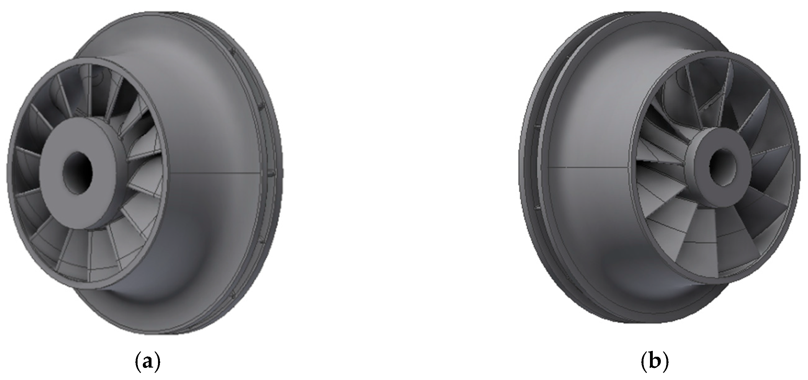
Optimization was conducted on a 100 kW organic Rankine cycle (ORC) turbine, utilizing waste heat from marine engines. As illustrated in Figure 1, the optimization was performed on the first-stage and second-stage rotors. As shown in

Table 1. Turbine parameters.

Parameter	First Stage	Second Stage
Inlet total pressure	2094.0 kPa	724.2 kPa
Inlet total temperature	155.0 °C	121.0 °C
Outlet total pressure	724.2 kPa	250.5 kPa
Outlet total temperature	121.0 °C	97.5 °C
Pressure ratio	2.9	2.9
Working fluid	R1233zd(E)	R1233zd(E)
Mass flow rate	4.2 kg/s	4.2 kg/s
Isentropic efficiency	91.1%	86.4%
Rotational speed	25,500 rpm	25,500 rpm
Power	79 kW	73 kW

, the turbine was designed to achieve the 100 kW output with R1233zd(E) as the working fluid, operating at a rotational speed of 25,500 rpm. For the first stage, the inlet temperature, inlet total pressure, and outlet total pressure were 155 °C, 2094 kPa, and 724.2 kPa (expansion ratio 2.9), respectively, while, for the second stage, they were 97.5 °C, 724.2 kPa, and 250.5 kPa.

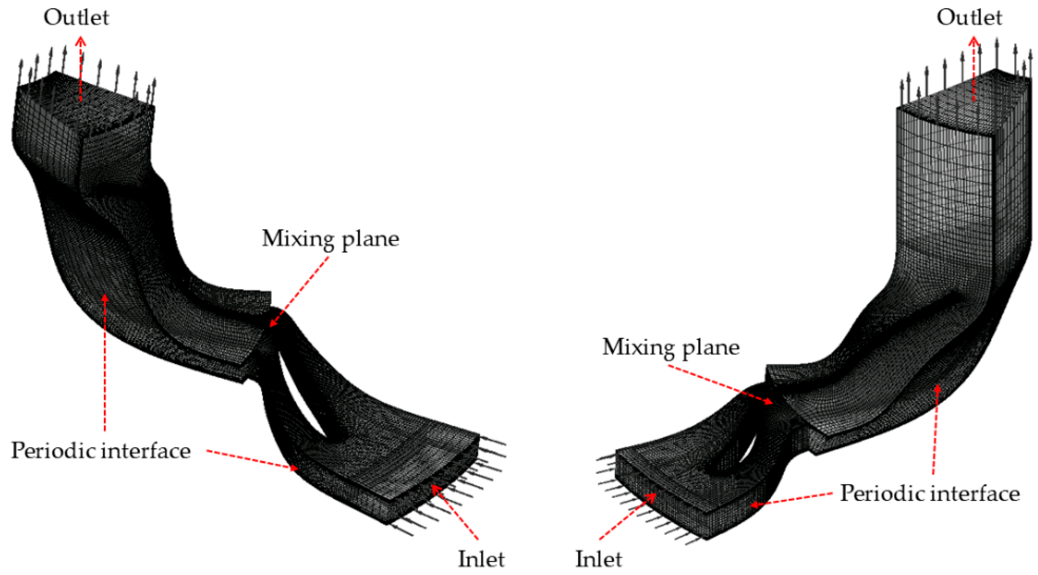
The computational domain was divided into four regions: inlet, nozzle, rotor, and outlet. The Shear Stress Transport (SST) turbulence model was employed for numerical analysis. As shown in Figure 2, a mixing-plane interface condition was applied between the nozzle and rotor regions, while periodic boundary conditions were imposed in the circumferential direction. The inlet and outlet were defined by total pressure and static pressure boundary conditions, respectively, corresponding to the specified operating conditions. The working fluid, R1233zd(E), had its thermophysical properties evaluated using the Peng–Robinson equation of state. Under these conditions, CFD was conducted and the total-to-total isentropic efficiencies were obtained as 91.1% for the first stage and 86.4% for the second stage.

2.2. Grid Dependency and Discretization

A grid dependency assessment was conducted using residual convergence and the grid convergence index (GCI) [11]. For the first stage, three grid systems consisting of approximately 0.55, 1.38, and 3.40 million nodes ($N_1$, $N_2$, and $N_3$) were examined in a previous study [12]. The GCI evaluated between the N₂ and N₃ grids yielded 0.75% for the mass flow rate, 0.01% for the total-to-total isentropic efficiency, and 0.02% for the outlet total enthalpy, confirming negligible discretization uncertainty. Based on this verification, the $N_1$ grid configuration was adopted for the first-stage simulations, consistent with the previous study.

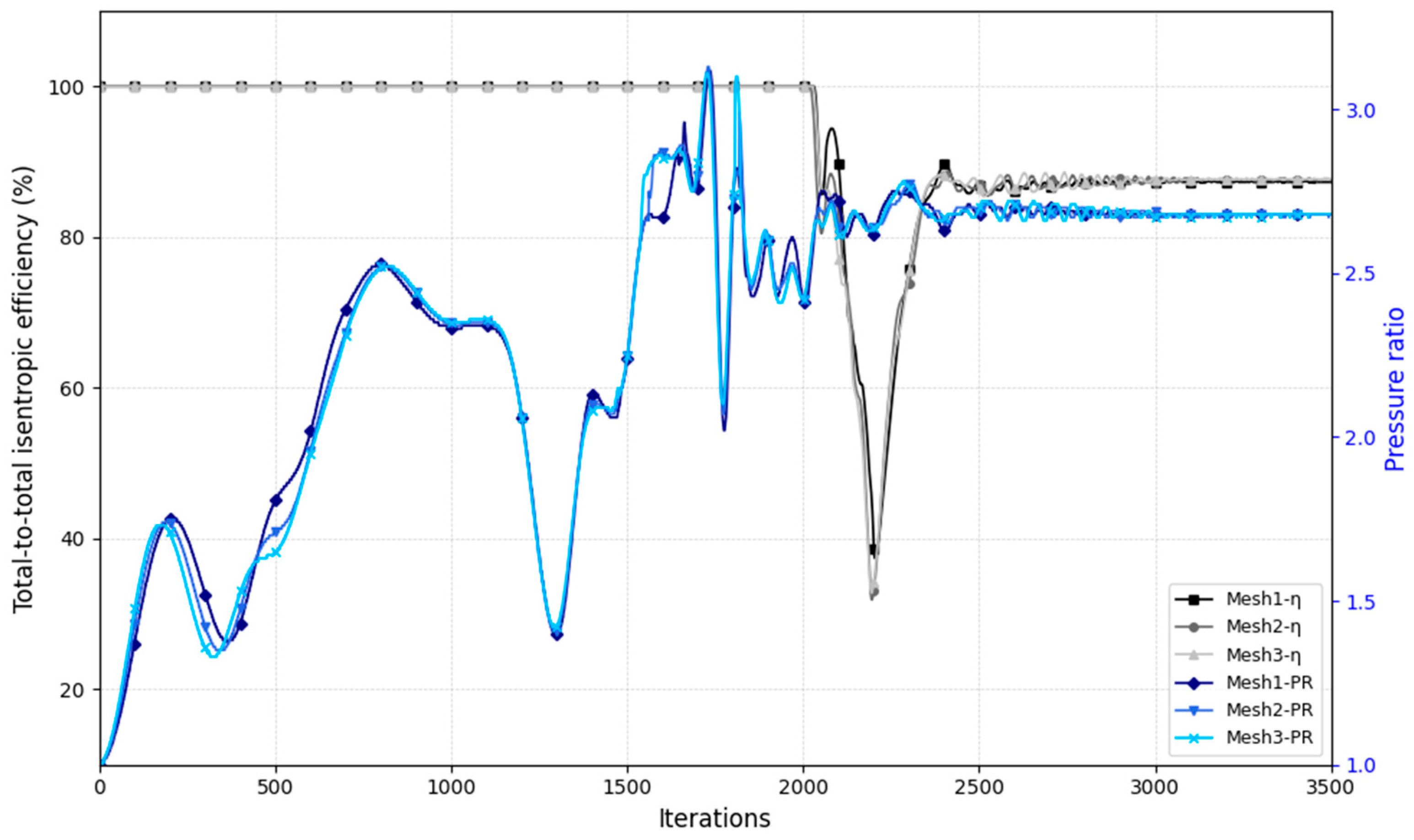
For the second stage, a grid dependency test was performed using three mesh systems (Mesh 1, Mesh 2, and Mesh 3). Figure 3 shows the convergence behavior of the total-to-total isentropic efficiency and pressure ratio. All mesh configurations reached stable convergence after approximately 3000 iterations, and no divergent trend was observed among the mesh levels.

The averaged RMS residuals at the end of the iterations are summarized in

Table 2. Averaged RMS residual distribution at the end of iterations.

	Mesh 1	Mesh 2	Mesh 3
Mass	7.82 × 10−6	1.33 × 10−5	1.92 × 10−5
U	1.97 × 10−4	2.50 × 10−4	2.06 × 10−4
V	1.40 × 10−4	1.73 × 10−4	1.55 × 10−4
W	2.36 × 10−4	3.05 × 10−4	2.39 × 10−4

. The residuals for mass conservation were on the order of 10⁻⁶–10⁻⁵, while the momentum residuals (U, V, and W) were on the order of 10⁻⁴, indicating satisfactory numerical convergence for all mesh systems.

Discretization uncertainty was quantified through GCI analysis [13]. The grid refinement ratio $r$ between successive mesh levels was set to approximately 1.35, satisfying the commonly recommended threshold of $r\ge 1.3$ for the reliable estimation of discretization errors. In

Table 3. Grid convergence index to evaluate discretization error.

	Mass Flow Rate (kg/s)	Shaft Power (W)	${\mathit{\eta }}_{\mathit{t}\mathit{t},\mathit{s}}$
$r_{21}$	1.369	1.369	1.369
$r_{32}$	1.342	1.342	1.342
${\mathrm{\Phi }}_1$	4.1447	74,281.7	0.865793
${\mathrm{\Phi }}_2$	4.1416	74,519.7	0.867650
${\mathrm{\Phi }}_3$	4.1407	74,697.9	0.868904
${\epsilon }_{21}$	−0.0031	238.0	0.001856
${\epsilon }_{32}$	−0.0009	178.2	0.001254
$s$	1	1	1
$p$	4.07	0.95	1.29
${\mathrm{\Phi }}_{\mathrm{e}\mathrm{x}\mathrm{t}}^{21}$	4.1404	75,203.4	0.871369
$e_a^{21}$	0.07%	0.32%	0.21%
$e_{ext}^{21}$	0.03%	0.91%	0.43%
$GC{I}_{fine}^{21}$	0.04%	1.15%	0.54%
${\mathrm{\Phi }}_{\mathrm{e}\mathrm{x}\mathrm{t}}^{32}$	4.1403	75,249.3	0.871619
$e_a^{32}$	0.02%	0.24%	0.14%
$e_{ext}^{32}$	0.01%	0.73%	0.31%
$GC{I}_{fine}^{32}$	0.01%	0.92%	0.39%

, ${\mathrm{\Phi }}_1$, ${\mathrm{\Phi }}_2$, and ${\mathrm{\Phi }}_3$ denote the computed values obtained from Mesh 1, Mesh 2, and Mesh 3, respectively, and $\epsilon$ represents the approximate relative error between adjacent meshes. The observed order of accuracy is denoted by $p$, and $s$ denotes the sign of the relative error used in the extrapolation process. The extrapolated value ${\mathrm{\Phi }}_{ext}$ represents the estimated solution at zero grid spacing, and $e_{ext}$ quantifies the relative deviation from this asymptotic value.

As summarized in Table 3, the GCI values between Mesh 2 and Mesh 3 were 0.01% for the mass flow rate, 0.92% for the shaft power, and 0.39% for the total-to-total isentropic efficiency. Between Mesh 1 and Mesh 2, the corresponding values were 0.04%, 1.15%, and 0.54%, respectively. Since the discretization uncertainty of the primary performance metric—the total-to-total isentropic efficiency—remained below 0.6% across the mesh comparisons, the numerical solution was considered sufficiently grid-independent for the present analysis. The selected mesh configuration was therefore employed for subsequent optimization analyses.

Four different surrogate models were used in the optimization framework, and the post-optimization blade geometries were evaluated and validated using an identical numerical analysis setup. The computational setup, including the grid model (size, type, and distribution), turbulence model, inlet and outlet boundary conditions, and interface configurations, was kept consistent across all cases. Accordingly, additional grid dependency analysis was not performed, as the same numerical settings and mesh strategy were consistently applied. The only varying factor among the cases was the blade geometry derived from each model.

2.3. Turbine Design Parameter

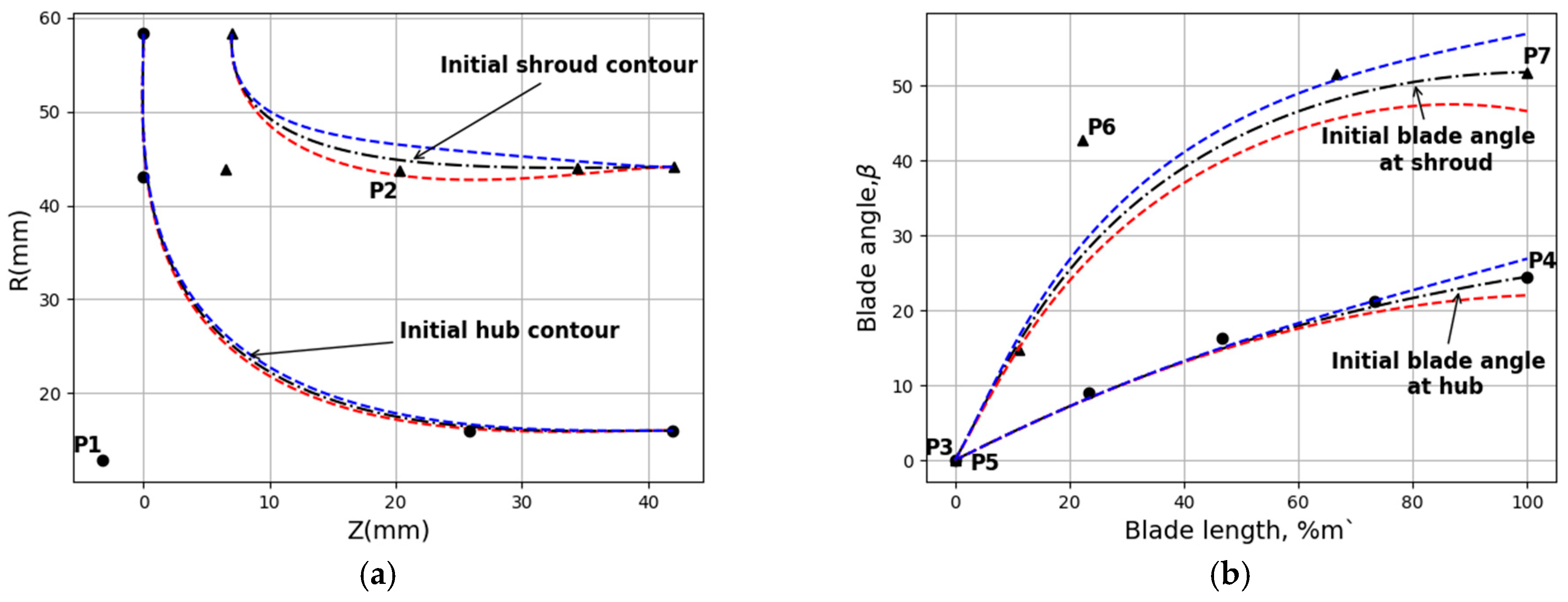
To enhance turbine performance while maintaining stable operating conditions, appropriate geometric parameters were selected to modify the blade shape under realistic geometric constraints. In this study, the turbine geometry was parameterized using Bézier curves following the approach adopted in Cho et al. [14], and selected control points were defined as design points for both the first and second stages.

In the meridional plane, the mid-span points (P1 and P2) were selected as design points. Geometric modifications near the inlet and outlet regions can significantly affect the effective flow area and may consequently alter the operating conditions of the turbine. To minimize such effects, these design points were constrained to move only in the axial (Z) direction, and their displacement was limited to ±10% of the baseline geometry.

In the β–%m′ plane, blade angle control points were selected to adjust blade turning without modifying the meridional flow path. The hub inlet and outlet points (P3 and P4), together with the shroud inlet, mid-span, and outlet points (P5, P6, and P7), were defined as design points. Excessive blade turning, particularly in the endwall regions, is known to intensify secondary flows and increase aerodynamic losses due to boundary layer growth and corner separation [15]. Therefore, to prevent abrupt turning variations while maintaining geometric feasibility, the allowable displacement of all design points was restricted to within ±10% of the baseline configuration, ensuring aerodynamic stability and physically realizable blade geometries.

Table 4. Design points for first stage and second stage.

First Stage				Second Stage
	Lower Limit	Base	Upper Limit		Lower Limit	Base	Upper Limit
P1	14.76 mm	16.4 mm	18.04 mm	P1	11.56 mm	12.8 mm	14.13 mm
P2	33.45 mm	37.2 mm	40.88 mm	P2	39.32 mm	43.7 mm	48.06 mm
P3	3.62°	4°	4.42°	P3	0°	0°	0°
P4	−60.40°	−54.9°	−49.42°	P4	22.02°	24.5°	26.91°
P5	7.40°	8.2°	9.04°	P5	0°	0°	0°
P6	−6.32°	−5.7°	−5.17°	P6	38.40°	42.7°	46.94°
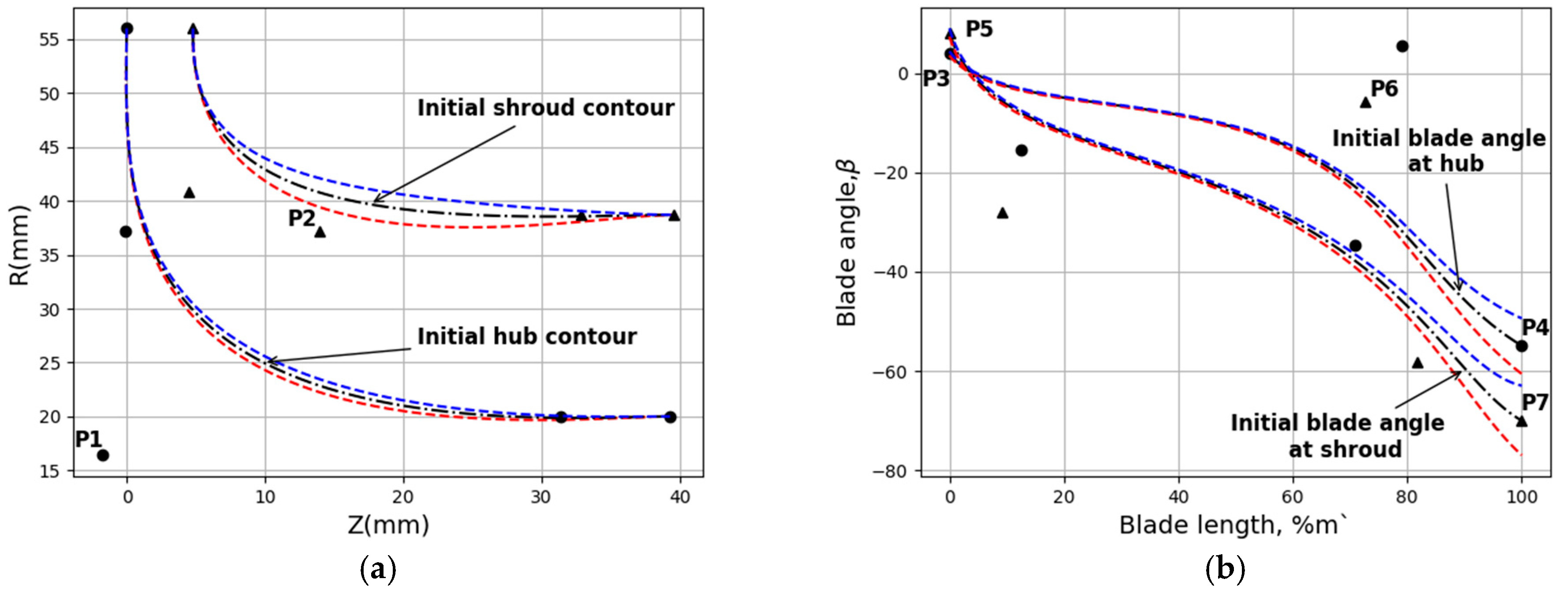
P7	−76.96°	−70°	−62.97°	P7	46.59°	51.8°	56.94°

summarizes the baseline coordinates and corresponding upper and lower bounds of all design points, while Figure 4 and Figure 5 illustrate the baseline geometry and the maximum and minimum geometries obtained through the variation of these points for both turbine stages.

2.4. Objective Function

In turbine optimization, various objective functions—such as the output power, pressure ratio, and isentropic efficiency—can be used depending on the research objective. In this study, the total-to-total isentropic efficiency, which most directly reflects the performance of the ORC turbine, was adopted as the objective function. The isentropic efficiency is defined by comparing the actual rotor exit enthalpy with the ideal exit enthalpy obtained under an isentropic process, as shown in Equation (1):

$${\eta }_{tt,\mathrm{i}s}={\displaystyle \frac{h_1-h_{2,a}}{h_1-h_{2,s}}}$$

(1)

Here, $h_1$ denotes the nozzle inlet enthalpy, $h_{2,a}$ represents the actual rotor exit enthalpy, and $h_{2,s}$ indicates the ideal isentropic exit enthalpy. Since the isentropic efficiency quantitatively reflects the losses that occur during the actual process, it is suitable for evaluating the optimization effects related to internal flow characteristics and loss mechanisms within the turbine. In this study, optimization focused on minimizing internal losses and enhancing output performance under fixed operating and mass flow conditions. Accordingly, the total-to-total isentropic efficiency was selected as the single objective function, as it effectively represents both loss reduction and power improvement within the turbine.

2.5. Optimization Methodology

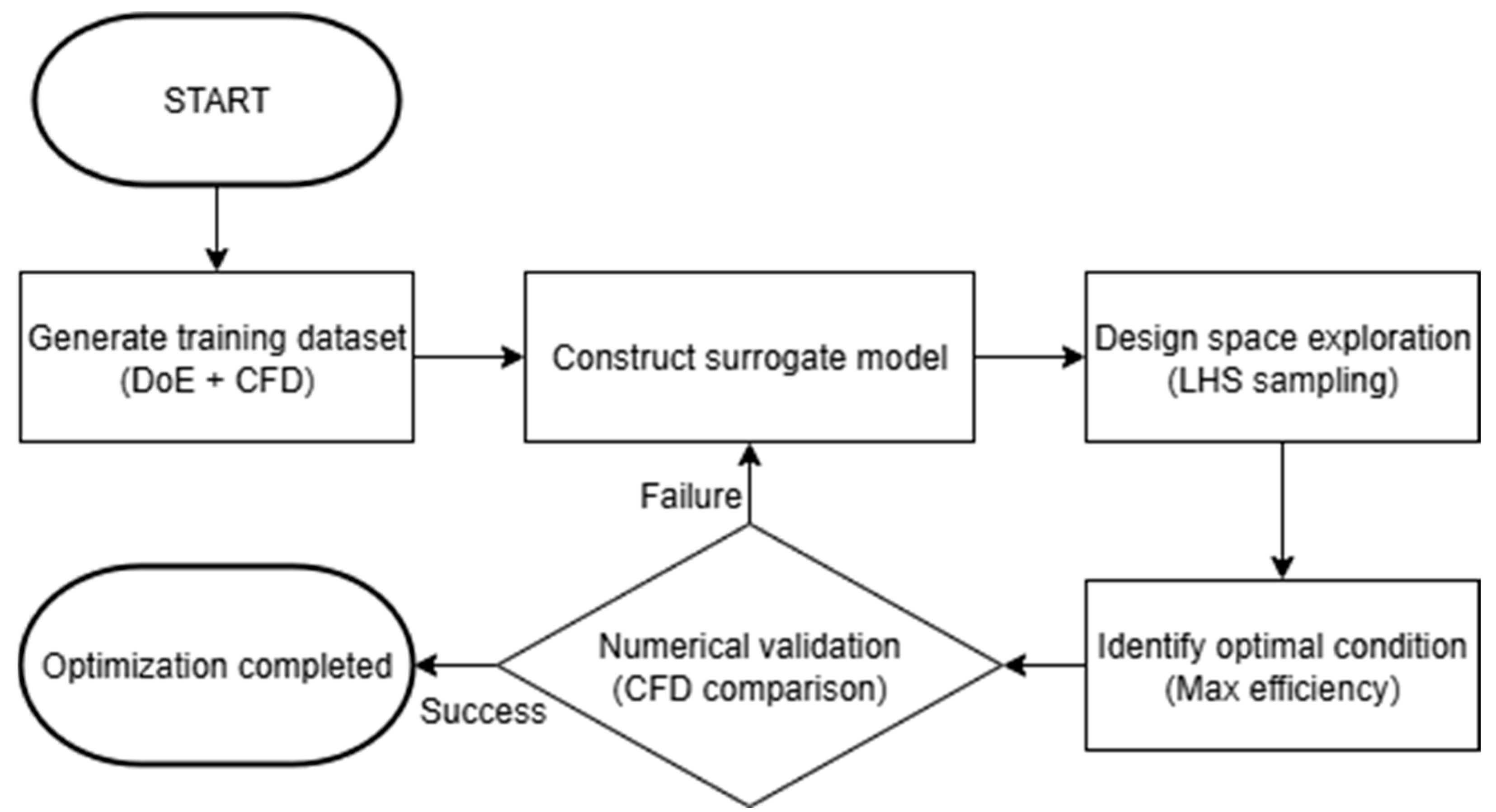
Figure 6 illustrates the overall surrogate-based optimization procedure adopted in this study. To perform optimization using surrogate models, appropriate training data must be prepared. In this study, seven design variables were normalized to a range of −1 to 1, and combinations of −1 and 1 were assigned to each variable to generate the geometric configurations. Normalization was applied to prevent distortion caused by differences in the magnitudes of the design variables. Numerical analyses were then conducted for each generated configuration to evaluate the objective function, and the resulting data were combined with the seven corresponding design variables to form individual training samples. A total of 64 training samples were ultimately constructed and utilized for training the surrogate models.

Using the constructed training data, surrogate models for the ORC turbine were developed. Each surrogate model was trained to predict the objective function corresponding to a given geometric configuration. The design variable bounds are listed in Table 4. To efficiently explore the admissible space, Latin hypercube sampling (LHS) was employed to generate 48,000 candidate design points within these bounds. For each candidate, the surrogate model predicted the objective (total-to-total isentropic efficiency). The configuration with the highest predicted efficiency was then selected and evaluated through high-fidelity numerical analysis to obtain the CFD-predicted efficiency, which was then compared with the surrogate prediction to validate the optimization results.

For each stage, an independent training dataset consisting of 64 CFD samples was generated using the same design variable definitions and sampling strategy. Therefore, the first- and second-stage rotors were optimized independently. Separate surrogate models were trained for each stage and applied only to the corresponding optimization process. This approach was adopted to examine whether the comparative performance trends of the surrogate models remained consistent when the training datasets were independently generated under identical sampling strategies and design variable settings.

2.6. Surrogate Models

The optimization of the ORC turbine requires substantial computational resources due to its iterative numerical analysis process. To lower the computational cost, surrogate models were employed to approximate the relationships between the design parameters and the objective function using limited training data. The principles and theoretical bases of the four surrogate models used are described in this section. All surrogate models were implemented using built-in functions in MATLAB R2021a.

2.6.1. Radial Basis Neural Network

Orr [16] defined the radial basis neural network (RBNN) as a neural network that approximates the input–output relationship using radial basis functions in the hidden layer. The basic structure of an RBNN is composed of an input layer, a hidden layer, and an output layer. The hidden layer performs nonlinear transformations, while the output layer generates the final output through a linear combination. The output of the network is expressed as shown in Equation (2):

$$y\left(x\right)= \sum _{i=1}^N{w}_i\varphi \left(\left|x-c_i\right|\right), \varphi \left(r\right)=\mathrm{e}\mathrm{x}\mathrm{p}\left(-{\displaystyle \frac{r^2}{2{\sigma }_i^2}}\right)$$

(2)

where, $c_i$ denotes the center (centroid), ${\sigma }_i$ the spread, $w_i$ the trained weight, and $N$ the number of radial basis functions (or centers) in the hidden layer. This structure possesses local approximation characteristics, allowing it to achieve high predictive performance even for complex nonlinear systems.

In the RBNN model, the spread constant (sc) and the target error goal (eg) are treated as hyperparameters because they are not directly estimated from the training data but instead govern the basis function width and the training stopping criterion. The spread constant controls the locality and smoothness of the radial basis functions, while the error goal defines the target mean squared error threshold used to terminate neuron growth. These parameters significantly influence model complexity and generalization behavior.

To identify suitable hyperparameter values while reducing the risk of overfitting, a K-fold cross-validation procedure was applied. For each candidate combination of sc and eg, the model was repeatedly trained and validated on independent data partitions, and the predictive performance was evaluated using the root mean squared error (RMSE) and the coefficient of determination (R²). The hyperparameter set showing a low RMSE and high R² was selected. Based on the cross-validation results, the selected hyperparameter values for the RBNN models were sc = 9.0 and eg = 0.01 for the first stage and sc = 9.3 and eg = 0.02 for the second stage. The rationale for the chosen number of folds and the statistical adequacy of the training dataset are discussed later based on the learning curve analysis.

2.6.2. Response Surface Approximation

Box and Wilson [17] proposed response surface approximation (RSA) as a method for approximating the relationships between design variables and responses using polynomial regression. A general second-order polynomial-based RSA is expressed as shown in Equation (3):

$$y\left(x\right)={\beta }_0+ \sum _{i=1}^k{\beta }_i{x}_i+ \sum _{i=1}^k{\beta }_{ii}{x}_i^2+\sum _{i<j}{\beta }_{ij}{x}_i{x}_j$$

(3)

where ${\beta }_0,{\beta }_i,{\beta }_{ii},{\beta }_{ij}$ represent the regression coefficients, and $x_i$ denotes the design variables. RSA offers the advantages of a very low computational cost and the ability to rapidly capture the global trends of the overall design space. These characteristics make it particularly useful in the early stage of design or for exploring large design spaces. However, since it is fundamentally based on polynomial regression, its accuracy tends to decrease when dealing with strongly nonlinear problems, and it is vulnerable to extrapolation outside the design space.

2.6.3. Kriging

Sacks et al. [18] defined Kriging as a stochastic interpolation method that predicts the response at any design point through the combination of a mean function and a covariance structure. Kriging integrates regression and interpolation to predict values along with their uncertainties. The general predictive formulation of Kriging is expressed as shown in Equation (4):

$$\widehat{y}= \mu +r{\left(x\right)}^T{R}^{-1}(y-\mu {\mathbf{1}}_{\mathit{n}})$$

(4)

where μ is the global mean, r(x) is the correlation vector between the prediction point x and the training data, R is the correlation matrix, ${\mathbf{1}}_{\mathit{n}}$ denotes an n-dimensional vector of ones, y is the vector of training responses, and $\widehat{y}$ is the predicted response. Since Kriging models the spatial correlations among data points, it provides stable predictive performance even in cases with high local variability or complex design spaces. Moreover, because Kriging yields both predicted values and their associated variance (uncertainty), it is particularly effective for reliability-based exploration during the optimization process.

2.6.4. PRESS-Based Weighted Ensemble

In general, it is difficult to determine in advance which surrogate model is the most suitable for a given application. Each surrogate model exhibits different predictive characteristics depending on the functional nonlinearity and data distribution. Therefore, combining multiple surrogate models through a weighted average model can provide a more stable and robust prediction. The general form of the weighted average model is shown in Equation (5):

$${\widehat{y}}_{wt.avg}\left(x\right)= \sum _1^{N_{SM}}{w}_i\widehat{y_i}\left(x\right), \sum _{i=1}^{N_{SM}}{w}_i=1$$

(5)

where ${\widehat{y}}_{wt.avg}\left(x\right)$ denotes the weighted average prediction, $\widehat{y_i}\left(x\right)$ represents the prediction of the i-th surrogate model, and $w_i$ is the corresponding weight. The weights were determined using a PRESS-based weighted (PBW) approach The generalization performance of each surrogate model was evaluated using leave-one-out cross-validation (PRESS). The cross-validated RMSE for the $i$-th surrogate model is computed as

$$E_i=\sqrt{{\displaystyle \frac{1}{n}}\sum _{k=1}^n{\left(y_k-{\widehat{y}}_{-k}^{\left(i\right)}\left(x_k\right)\right)}^2}$$

(6)

where ${\widehat{y}}_{-k}^{\left(i\right)}\left(x_k\right)$ denotes the prediction of the $i$-th surrogate model trained without the $k$-th sample. The weights were then calculated as

$$\begin{gathered} w_i^{*}={\left(E_i+\alpha E_{avg}\right)}^{\beta }, w_i=w_i^{*}/\sum _i{w}_i^{*} \\ {E}_{avg}= {\sum }_{i=1}^{N_{SM}}{E}_i /{ N}_{SM}; \beta <0, \alpha <1 \end{gathered}$$

(7)

In this study, the parameters were set to $\alpha =0.05$ and $\beta =-1$ [19]. Since $\beta <0$, surrogate models with a smaller RMSE receive larger weights. The $\alpha E_{avg}$ term prevents the excessive dominance of a single model and enhances numerical stability.

Unlike conventional preference-based averaging, the PBW method assigns weights objectively based on cross-validated generalization errors. This enables statistically grounded ensemble construction and improves the robustness under limited training data conditions.

2.7. Validation of Training Sample Size

Surrogate models exhibiting nonlinear characteristics, such as RBNN and Kriging models, may suffer from overfitting or underfitting when trained with insufficient data. Therefore, the adequacy of the 64 CFD training samples employed in this study was systematically evaluated.

The present optimization problem involves seven design variables. A full two-level factorial exploration at the extreme bounds would require $2^7=128$ design points. The 64 samples used in this study correspond to a half-fractional design scale. Fractional factorial designs are commonly adopted to efficiently capture dominant effects within a bounded design space while reducing the experimental cost [20]. However, such theoretical design considerations alone do not guarantee the predictive generalization of nonlinear surrogate models. Accordingly, empirical validation based on model performance was additionally performed.

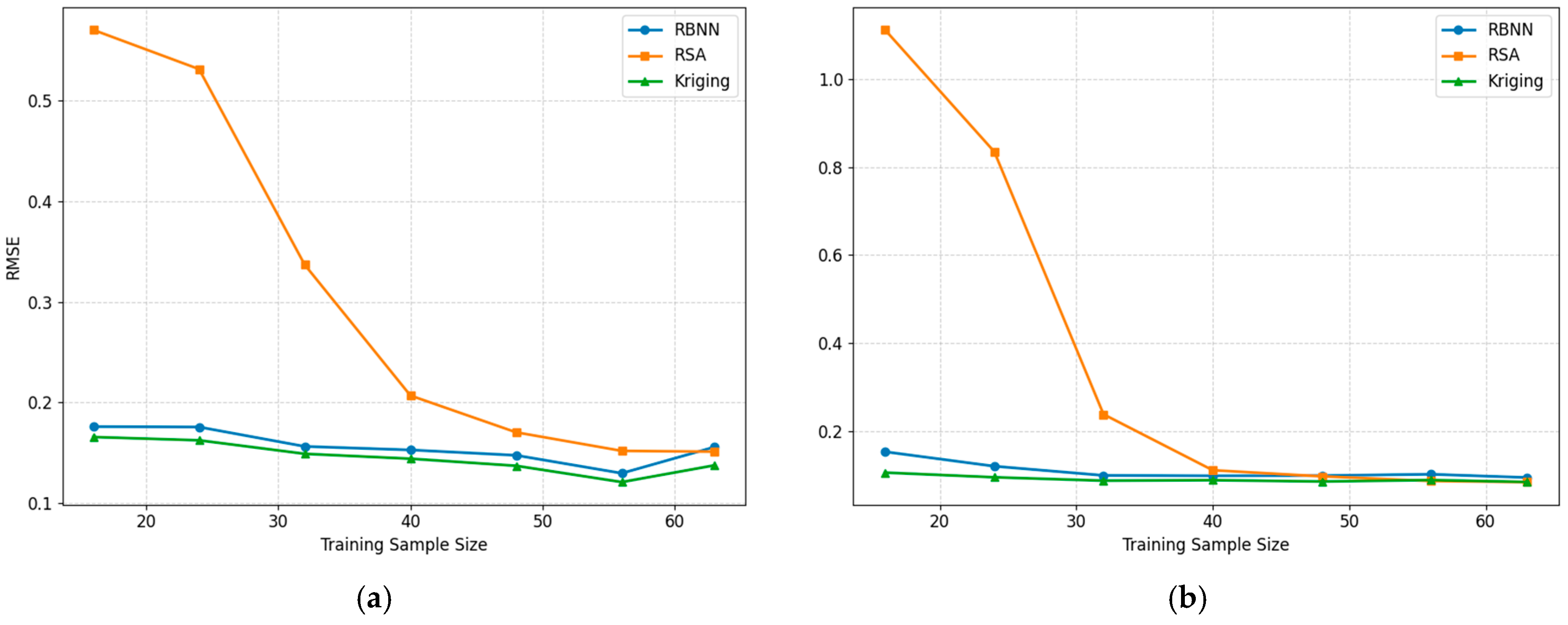
To quantitatively assess the influence of the training sample size on predictive performance, a learning curve analysis was conducted. The number of training samples $N_{\mathrm{train}}$ was gradually increased from 16 to 24, 32, 40, 48, 56, and 63. For each case, the remaining samples $\left(64−N_{\mathrm{train}}\right)$ were used as validation data, and the root mean square error (RMSE) was calculated as

$$\mathrm{R}\mathrm{M}\mathrm{S}\mathrm{E}({\mathrm{N}}_{\mathrm{t}\mathrm{r}\mathrm{a}\mathrm{i}\mathrm{n}})=\sqrt{{\displaystyle \frac{1}{N_{val}}}\sum _{\mathrm{i}=1}^{N_{val}}{\left(y_i^{CFD}-{\widehat{y}}_i\right)}^2}$$

(8)

where $N_{\mathrm{val}}=64-N_{\mathrm{train}}$, $y_i^{\mathrm{CFD}}$ denotes the CFD result, and ${\widehat{y}}_i$ represents the surrogate prediction. To reduce the bias arising from random data partitioning, each configuration was repeated $K=30$ times with independently randomized splits. The averaged RMSE was computed as

$$\overline{\mathrm{R}\mathrm{M}\mathrm{S}\mathrm{E}}({\mathrm{N}}_{\mathrm{t}\mathrm{r}\mathrm{a}\mathrm{i}\mathrm{n}})={\displaystyle \frac{1}{\mathrm{K}}}\sum _{k=1}^{K}RMS{E}_k$$

(9)

When 63 samples were used for training, leave-one-out cross-validation (LOOCV) was applied across all 64 samples.

The results show that the RMSE consistently decreases as the number of training samples increases for all surrogate models in both stages, as shown in Figure 7. Notably, the rate of RMSE reduction becomes markedly smaller beyond 56 training samples in the first stage and beyond 48 samples in the second stage, indicating a saturation trend. Furthermore, the difference between the averaged RMSE at 56 training samples and the LOOCV-based RMSE was limited, suggesting that additional data beyond this level provide only a marginal improvement in predictive accuracy. These observations indicate that 64 training samples result in a stable level of generalization performance.

To further interpret the different convergence behaviors observed between the two stages, design point sensitivity estimation based on the Kriging correlation parameters was performed following the framework of Loeppky et al. [21]. The Gaussian correlation function is expressed as

$$R\left(x,x^{\prime }\right)=\mathrm{e}\mathrm{x}\mathrm{p}(-\sum _{j=1}^d{\theta }_j{\left(x_j-x_j^{\prime }\right)}^2)$$

(10)

where d denotes the number of design points, ${\theta }_j=1/\left(2l_j^2\right)$, and $l_j$ denotes the correlation length scale in the $j$-th design direction. A larger ${\theta }_j$ corresponds to a shorter correlation length, implying more rapid variation in the response along this direction. The total sensitivity index was defined as

$$\tau =\sum {\theta }_j$$

(11)

As shown in

Table 5. Kriging correlation parameters (θ) and total sensitivity index (τ) used for design point sensitivity estimation in the first and second stages.

First Stage			Second Stage
	$\mathit{\theta }$	$\mathit{\tau }$		$\mathit{\theta }$	$\mathit{\tau }$
P1	0.1	6189.6	P1	0.04	30.66
P2	398.7		P2	4.32
P3	0.1		P3	0.06
P4	2445.6		P4	4.16
P5	0.0		P5	0.11
P6	0.0		P6	3.85
P7	3345.1		P7	18.11

, the first-stage model exhibited a substantially larger $\tau$ value than the second-stage model, indicating shorter correlation lengths and relatively stronger local variation in the response surface. In contrast, the second-stage model showed a smaller $\tau$, suggesting a comparatively smoother response surface. This tendency is consistent with the learning curve results, where the second-stage models demonstrated faster RMSE convergence, whereas the first-stage models required a larger number of samples to achieve comparable stabilization.

Based on both the learning curve analysis and the Kriging-based sensitivity estimation, the 64 CFD training samples employed in this study provided stable predictive behavior within the defined design bounds. The results indicate that, under the present sampling strategy and problem formulation, increasing the number of training samples beyond this level yields only marginal improvements in the predictive error.

3. Results and Discussion

3.1. Comparison of Surrogate Models for the First-Stage Rotor

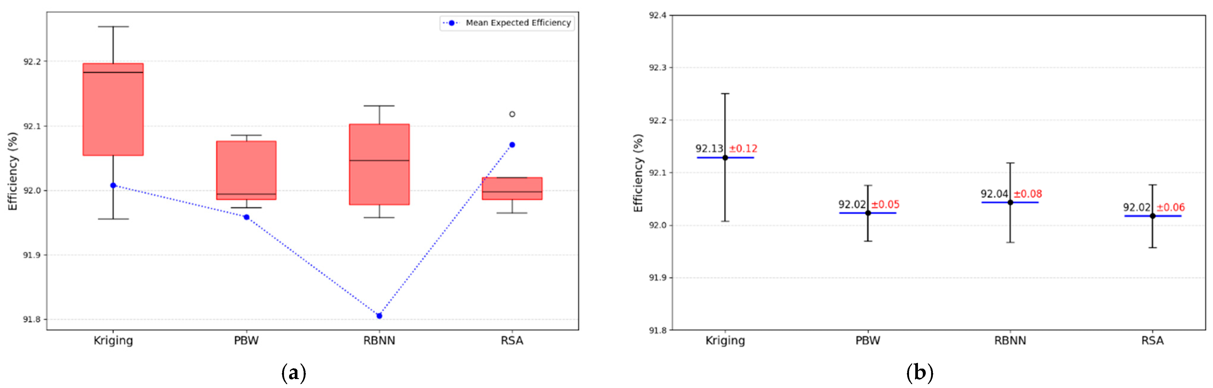
A surrogate model is a mathematical approximation of a complex physical or computational system. Since the input samples generated through LHS vary in each iteration, the optimal geometric configuration yielding the maximum efficiency may differ across independent runs. Therefore, to assess how accurately each surrogate model approximated the actual physical behavior, five independent optimization runs were conducted for each model. The surrogate-predicted efficiencies were compared with the corresponding CFD results to assess the prediction accuracy of each model.

As shown in

Table 6. Surrogate model predictions and numerical results for first-stage efficiency.

First-Stage Efficiency [%]
Model	Numerical Analysis	Surrogate Prediction	RMSE	Base
RBNN	92.04	91.81	0.250	91.1
RSA	92.02	92.07	0.073
Kriging	92.13	92.01	0.165
PBW	92.02	91.96	0.083

, the efficiencies predicted by the surrogate models (RBNN, RSA, Kriging, and PBW) were distributed within a narrow range of 91.8–92.1%. The corresponding CFD-validated efficiencies ranged from 92.02% to 92.13%, indicating that all surrogate models identified comparable high-performance regions within the design space.

To quantitatively evaluate the predictive accuracy, the RMSE between the surrogate predictions and CFD results was computed. RSA and PBW exhibited the lowest RMSE values, indicating superior predictive consistency. Kriging showed moderate errors, whereas the RBNN demonstrated comparatively larger deviations. In terms of prediction bias, RSA tended to overpredict the CFD results, while the RBNN, Kriging, and PBW slightly underpredicted the efficiency. However, the magnitude of these systematic deviations remained small relative to the overall efficiency improvement achieved through optimization.

Figure 8b presents the mean CFD efficiencies and their standard deviations for each model. Although the Kriging-based optimization achieved the highest mean CFD efficiency (92.13%), RSA and PBW demonstrated smaller dispersion and lower prediction errors. These results suggest that, in the first-stage optimization, Kriging was effective in locating slightly higher-performance designs, whereas RSA and PBW provided more stable predictive behavior.

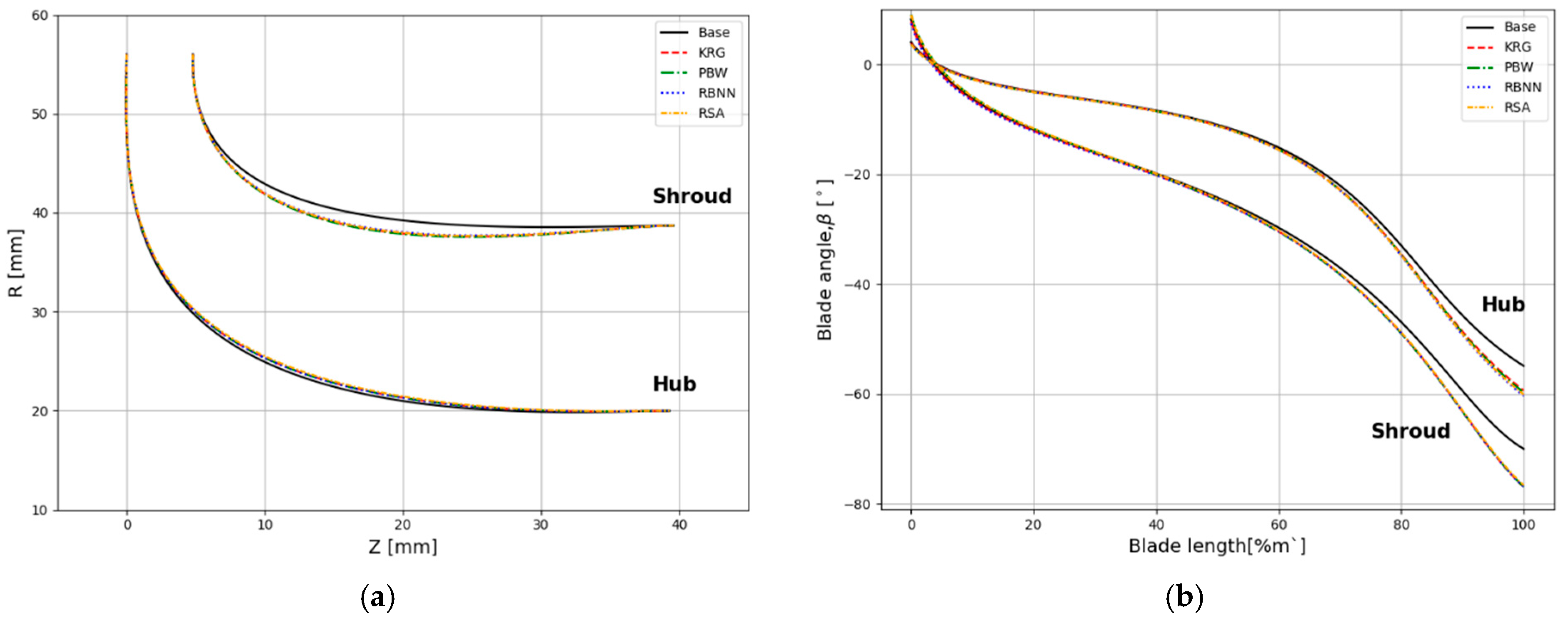
In the first stage of the ORC turbine, the surrogate-based optimization resulted in an efficiency improvement of approximately 0.9–1% compared with the baseline. Since the optimization was achieved through the modification of the geometric design points, the corresponding shape variations were examined. Figure 9 illustrates the Bézier curves of the optimized geometries—specifically, the cases with the highest CFD-validated efficiency among the five independent runs for each model—compared with the baseline geometry.

In the meridional plane, the hub surface exhibited a slight displacement in the +R direction, whereas the shroud surface showed a tendency to shift in the −R direction. In terms of blade angle variation, most design points demonstrated only minor changes; however, a pronounced reduction in the blade outlet angle was observed. Although small differences existed among the surrogate models, consistent trends in geometric modification were identified across all optimization cases.

Based on the Kriging-based design point sensitivity estimation, P2, P4, and P7 were identified as the dominant design points in the first-stage optimization. As shown in Figure 7, the shroud geometry corresponding to P2 exhibited a noticeable reduction, while P1, which showed relatively low sensitivity, remained nearly unchanged. Similarly, significant decreases in the outlet blade angle associated with P4 and P7 were observed, whereas only minor variations were detected for P3, P5, and P6. These observations are consistent with the previously estimated sensitivity indices, confirming that the geometric modifications were primarily concentrated in the most influential design points.

The dominance of P2, P4, and P7 indicates that the objective function exhibits relatively stronger local sensitivity around these design points, suggesting localized variations in the response surface within the defined design bounds. In the first-stage case, surrogate models with flexible correlation structures, such as Kriging, identified designs with slightly higher CFD-validated efficiency compared to the other models. The RBNN model exhibited comparatively larger RMSE values in this stage, indicating less consistent predictive performance under the present training conditions. In contrast, RSA and the PBW model showed smaller RMSE values, suggesting more stable error characteristics, although the differences among models remained limited in magnitude.

3.2. Comparison of Surrogate Models for the Second-Stage Rotor

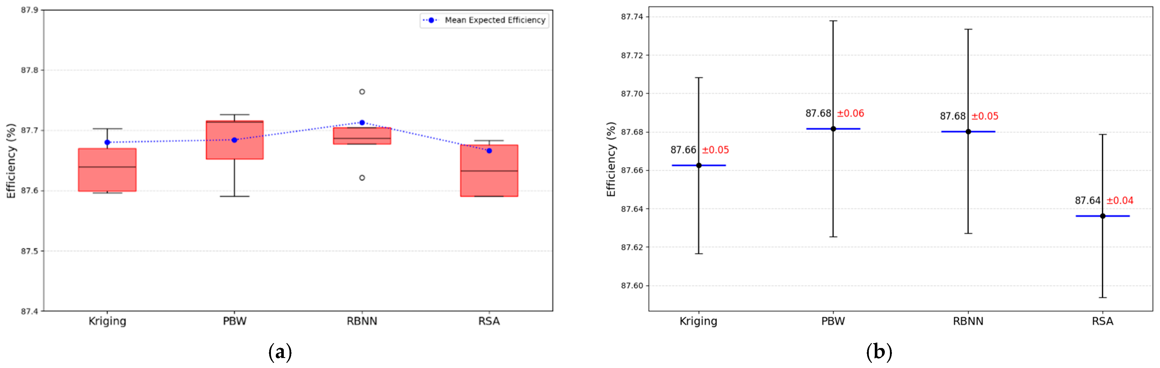
In the second-stage optimization, as shown in Figure 10, the efficiencies predicted by the surrogate models (RBNN, RSA, Kriging, and PBW) were distributed within a narrow range of 87.66–87.71%, indicating that all models converged to closely similar optimal solutions. The corresponding CFD-validated efficiencies ranged from 87.64% to 87.68%, demonstrating that the optimized designs identified by each surrogate model achieved nearly identical performance levels.

To quantitatively evaluate the predictive accuracy, the RMSE between the surrogate predictions and CFD results was calculated. Kriging exhibited the lowest RMSE (0.043), followed by RSA (0.047) and PBW (0.054), while the RBNN showed a slightly higher value (0.062). Overall, the RMSE values in the second stage were considerably lower than those observed in the first stage, indicating improved predictive agreement among models. When comparing the mean efficiencies, all surrogate models showed a slight tendency to overpredict the CFD results. However, the magnitude of deviation remained small across all cases, and no pronounced discrepancy among models was observed.

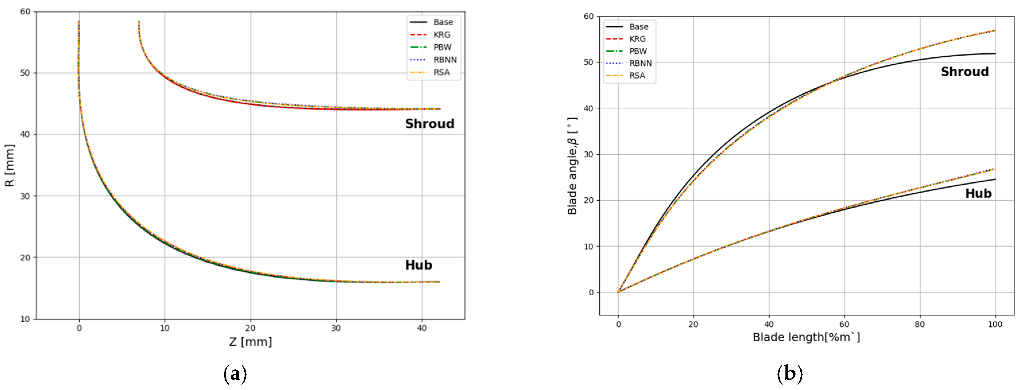
Figure 11 illustrates the geometric variations in both the meridional plane and the blade angle distribution for the second stage. In the meridional plane, the hub surface exhibited almost no deviation from the baseline geometry, while the shroud showed a slight displacement in the +R direction. In terms of blade angle variation, an increase in the outlet blade angles was observed for both the hub and shroud, whereas a reduction was identified at the mid-shroud design point.

Compared with the first-stage results, where small differences were primarily observed in the angular distribution among surrogate models, the second stage exhibited nearly identical angular profiles across models, with only slight variations in the meridional geometry. This suggests a more uniform geometric response to surrogate-based optimization in the second stage.

According to the design point sensitivity estimation, P2, P4, P6, and P7 were identified as dominant design points in the second stage. However, despite the high estimated sensitivity of P2, the corresponding geometric modification remained relatively small. In contrast, more noticeable changes were observed in the design points associated with P4, P6, and P7. This behavior suggests that, although P2 strongly influences efficiency, the allowable geometric variation around this design point may be limited within the optimal region.

Unlike the first stage, the second stage exhibited a lower overall total sensitivity index. This reduced sensitivity suggests that the local gradients of the response surface may be less steep, indicating a relatively smooth design space. Under such conditions, the surrogate models produced highly similar optimal solutions, consistent with the low RMSE values and minimal discrepancy among models, as shown in

Table 7. Surrogate model predictions and numerical results for second-stage efficiency.

Second-Stage Efficiency [%]
Model	Numerical Analysis	Surrogate Prediction	RMSE	Base
RBNN	87.68	87.71	0.062	86.4
RSA	87.64	87.66	0.047
Kriging	87.66	87.69	0.043
PBW	87.68	87.68	0.054

.

3.3. Flow Analysis

Using the surrogate models, the rotor geometry of the ORC turbine was optimized to enhance the total-to-total isentropic efficiency. The improvement was achieved through geometric modifications of the rotor blades, and statistical exploration of the design space was employed to identify configurations expected to yield the maximum efficiency. In this section, the physical mechanisms underlying the efficiency enhancement are examined through comparative flow-field analyses of the optimized and baseline geometries.

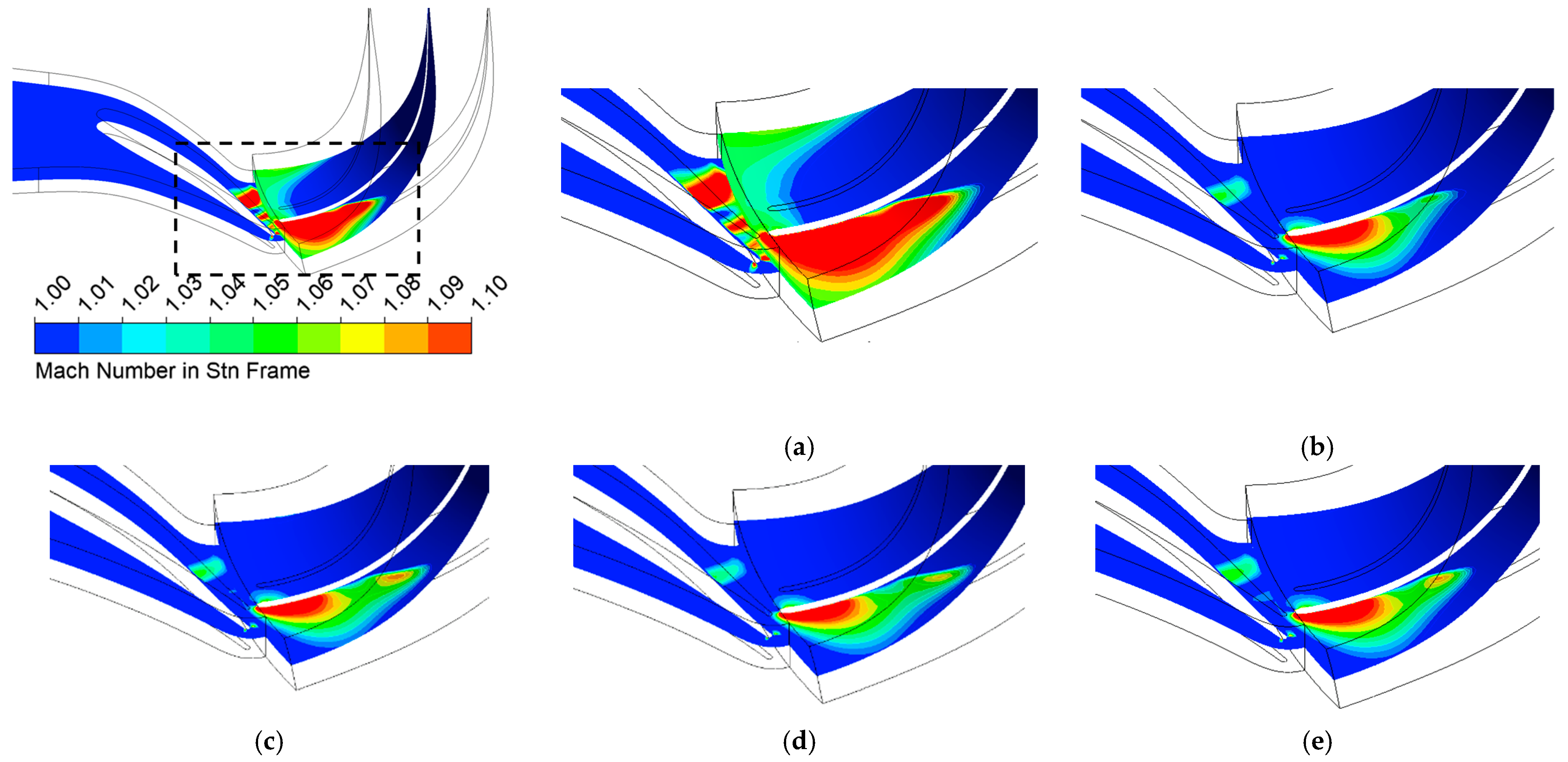
Mach number contours at the 50% span location were examined, with the range restricted to 1.0–1.1 in order to highlight the supersonic region where shock-related features are most evident. As presented in Figure 12, the spatial extent of the Mach 1.0–1.1 region in the first stage was reduced in the optimized cases compared with the baseline geometry. Since shock-induced compression and expansion processes are associated with irreversible losses, the contraction of this supersonic region suggests the possible weakening of shock-related dissipation within the rotor passage at the analyzed span location.

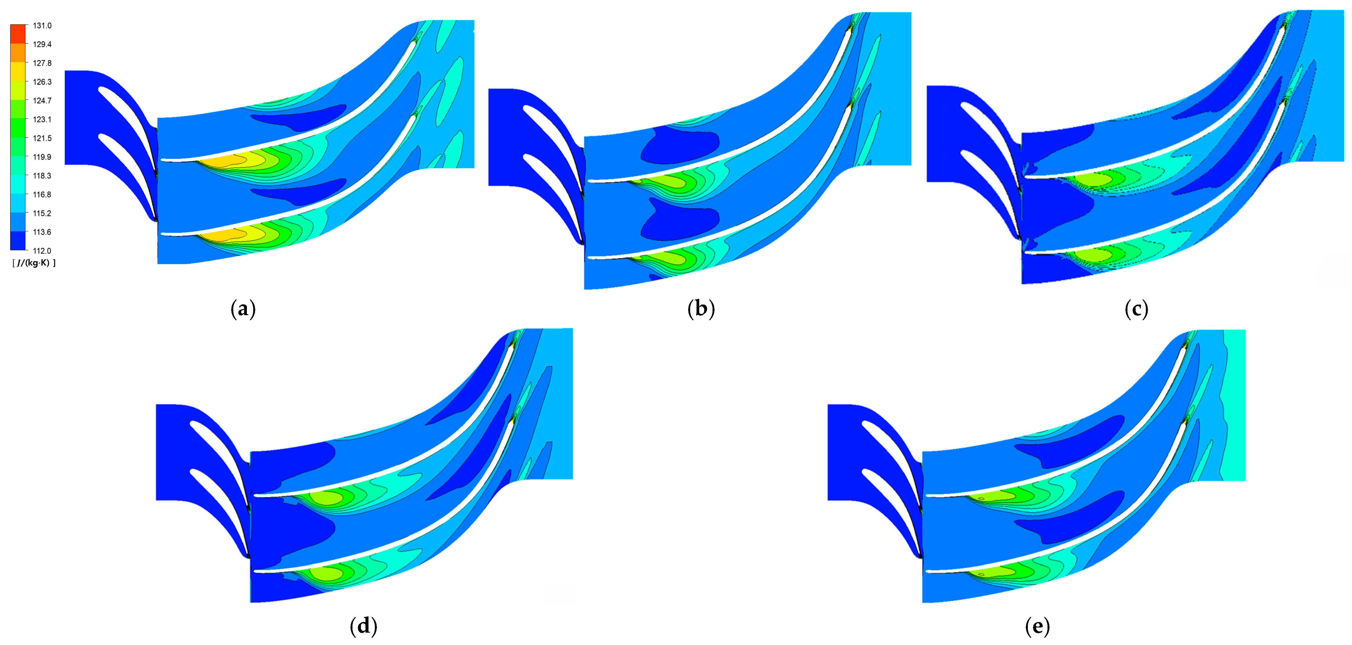
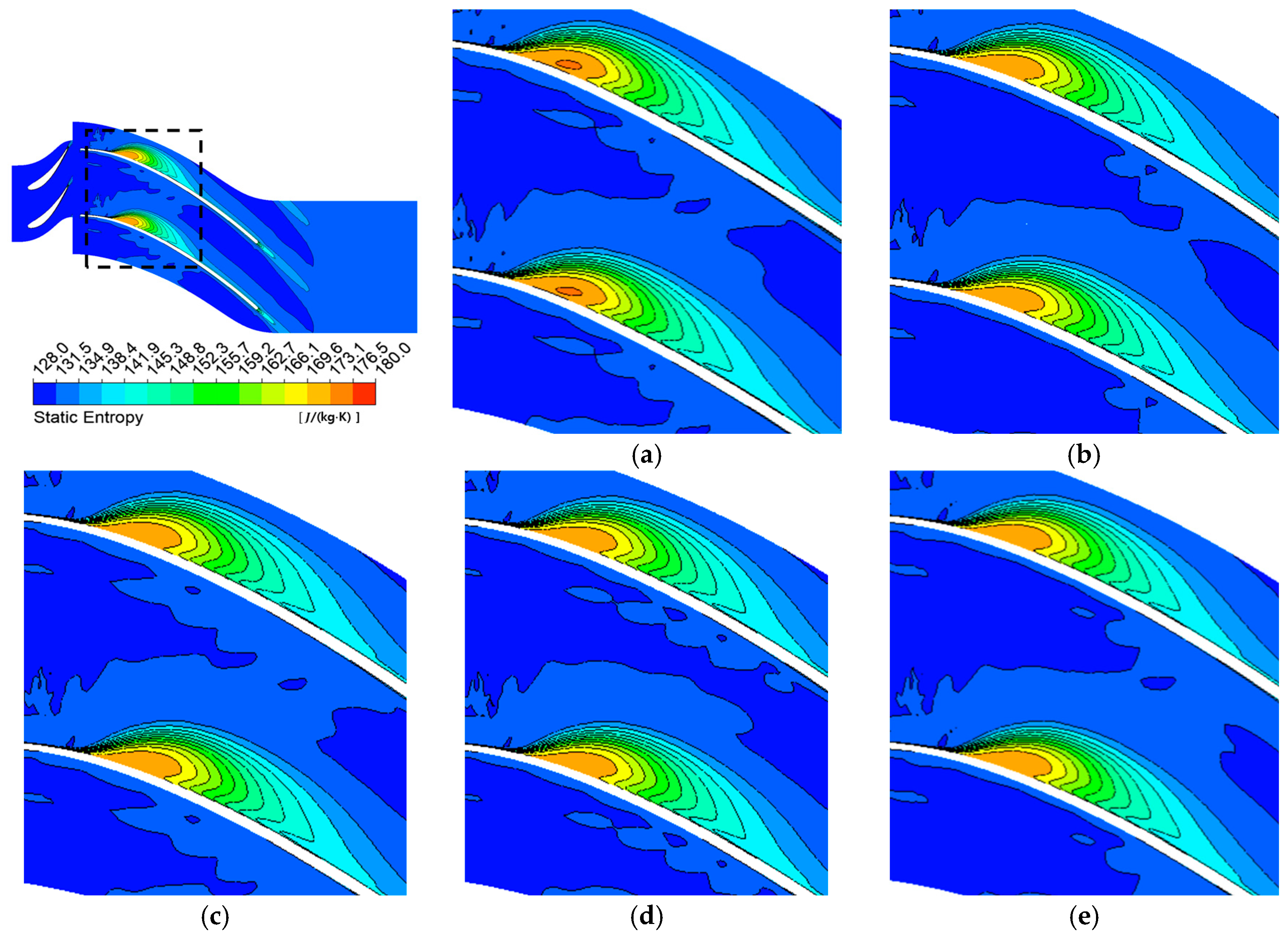
To further assess irreversible loss characteristics, static entropy contours were analyzed. Entropy generation represents thermodynamic dissipation within the flow field and is commonly used as an indicator of aerodynamic loss. As shown in Figure 13, the optimized first-stage geometries exhibited a reduction in both the spatial extent and magnitude of high-entropy regions near the trailing edge. This trend is qualitatively consistent with the observed modification of supersonic regions in the Mach number distribution.

In the second stage, as illustrated in Figure 14, the overall spatial extent of the high-entropy region remained comparable to that of the baseline case; however, the local entropy magnitude was reduced in the optimized configurations. Unlike the first stage, where the visible contraction of the supersonic region was observed, the second stage primarily exhibited a decrease in entropy intensity without a substantial qualitative change in the overall flow pattern at the 50% span. This suggests that the geometric modification in the second stage influenced local dissipation characteristics rather than significantly altering the global flow structure.

Because the total-to-total isentropic efficiency is closely related to the irreversible losses occurring within the rotor passage, the reduction in entropy magnitude observed in the optimized geometries is consistent with decreased thermodynamic dissipation. Although the present analysis is limited to qualitative comparisons at a representative span location, the consistent reduction in entropy intensity across the optimized cases supports the interpretation that the geometric modifications are associated with improved aerodynamic performance.

Furthermore, despite minor geometric differences among the optimized results obtained using different surrogate models, similar flow-field modification patterns were observed in all cases. In particular, reductions in entropy magnitude and the attenuation of shock-related features were consistently identified at the analyzed span location. This consistency suggests that the efficiency improvement is related to common geometric trends identified during the optimization process, rather than being dependent on a specific surrogate formulation.

4. Conclusions

To respond to the increasing demand for efficient energy utilization, this study performed surrogate-based aerodynamic optimization of a 100 kW ORC turbine rotor. Four representative surrogate models were applied under identical numerical conditions, and their predictive behavior and optimization characteristics were comparatively evaluated.

Independent optimizations were conducted for the first- and second-stage rotors, allowing the characteristics of two different design variable spaces to be examined. Sensitivity analysis revealed that the first stage exhibited relatively stronger local nonlinear behavior, whereas the second stage showed a smoother response surface. Under these different design space characteristics, the surrogate models demonstrated similar overall optimization trends, while their predictive stability varied depending on the sensitivity structure.

Geometric modifications were primarily concentrated in design variables with higher sensitivity. In both stages, noticeable changes were observed near the outlet blade angle, indicating its dominant influence on aerodynamic performance. Flow-field analysis further suggested that the optimized geometries were associated with reduced entropy generation near the trailing edge region, supporting the interpretation that aerodynamic loss was mitigated.

The training dataset was constructed using a fractional factorial design, which prohibited the exhaustive exploration of the full design space. Nevertheless, the learning curve analysis indicated that the selected sample size provided stable predictive performance within the bounded design region. This suggests that an appropriately constrained surrogate framework can achieve reliable optimization without requiring full factorial sampling.

The present study focused on aerodynamic performance improvement under a single design operating condition. Although off-design performance is an important consideration in practical ORC turbine operation, it was not investigated in the present work and remains a subject for future study. The extension of the proposed surrogate-based optimization framework to off-design operating conditions is expected to provide further insights into the robustness of optimized blade geometries.

In addition, the optimization framework considered only aerodynamic efficiency as a single objective under fixed structural and manufacturing constraints. Structural integrity, thermomechanical loading, and multiobjective trade-offs were not incorporated in the current formulation. Future research may extend the framework to multidisciplinary optimization, larger training datasets, and broader operating envelopes to further assess its generalization capabilities and practical applicability.

References

1. Tchanche, B.F.; Lambrinos, G.; Frangoudakis, A.; Papadakis, G. Low-grade heat conversion into power using organic Rankine cycles—A review of various applications. Renew. Sustain. Energy Rev. 2011, 15, 3963–3979. [Google Scholar] [CrossRef]
2. Lecompte, S.; Huisseune, H.; van den Broek, M.; Vanslambrouck, B.; De Paepe, M. Review of organic Rankine cycle (ORC) architectures for waste heat recovery. Renew. Sustain. Energy Rev. 2015, 47, 448–461. [Google Scholar] [CrossRef]
3. Misener, R.; Biegler, L. Formulating data-driven surrogate models for process optimization. Comput. Chem. Eng. 2023, 179, 108411. [Google Scholar] [CrossRef]
4. Fan, H.; Wang, C.; Li, S. Novel method for reliability optimization design based on rough set theory and hybrid surrogate model. Comput. Methods Appl. Mech. Eng. 2024, 429, 117170. [Google Scholar] [CrossRef]
5. Liu, X.; Yang, S.; Sun, H.; Wang, Z.; Guan, X.; Gu, Y.; Wang, Y. Review of deep learning-based aerodynamic shape surrogate models and optimization for airfoils and blade profiles. Phys. Fluids 2025, 37, 041304. [Google Scholar] [CrossRef]
6. Samad, A.; Kim, K.-Y.; Goel, T.; Haftka, R.T.; Shyy, W. Multiple surrogate modeling for axial compressor blade shape optimization. J. Propuls. Power 2008, 24, 301–310. [Google Scholar] [CrossRef]
7. Shyy, W.; Papila, N.; Vaidyanathan, R.; Tucker, K. Global design optimization for aerodynamics and rocket propulsion components. Prog. Aerosp. Sci. 2001, 37, 59–118. [Google Scholar] [CrossRef]
8. Bandini, A.; Cascino, A.; Meli, E.; Pinelli, L.; Marconcini, M. Improving aeromechanical performance of compressor rotor blisk with topology optimization. Energies 2024, 17, 1883. [Google Scholar] [CrossRef]
9. González-Barrio, H.; Calleja-Ochoa, A.; Lamikiz, A.; López de Lacalle, L.N. Manufacturing processes of integral blade rotors for turbomachinery: Processes and new approaches. Appl. Sci. 2020, 10, 3063. [Google Scholar] [CrossRef]
10. Cascino, A.; Meli, E.; Rindi, A.; Pucci, E.; Matoni, E. Experimental validation and dynamic analysis of additive manufacturing burner for gas turbine applications. Machines 2025, 13, 1111. [Google Scholar] [CrossRef]
11. Roache, P.J. Perspective: A method for uniform reporting of grid refinement studies. J. Fluids Eng. 1994, 116, 405–413. [Google Scholar] [CrossRef]
12. Seo, J.-B.; Lee, H.; Han, S.-J. A design optimization of organic Rankine cycle turbine blades with radial basis neural network. Energies 2024, 17, 26. [Google Scholar] [CrossRef]
13. Celik, I.B.; Ghia, U.; Roache, P.J.; Freitas, C.J.; Coleman, H.; Raad, P.E. Procedure for estimation and reporting of uncertainty due to discretization in CFD applications. J. Fluids Eng. 2008, 130, 078001. [Google Scholar] [CrossRef]
14. Cho, S.; Lee, Y.; Ahn, K.; Kim, Y. A study on the design method to optimize an impeller of centrifugal compressor. J. Korean Soc. Fluid Mach. 2013, 16, 11–16. [Google Scholar]
15. Dixon, S.L.; Hall, C.A. Fluid Mechanics and Thermodynamics of Turbomachinery, 7th ed.; Butterworth-Heinemann: Oxford, UK, 2014. [Google Scholar]
16. Orr, M.J.L. Introduction to Radial Basis Function Networks; University of Edinburgh: Edinburgh, UK, 1996. [Google Scholar]
17. Box, G.E.P.; Wilson, K.B. On the experimental attainment of optimum conditions. J. R. Stat. Soc. Ser. B 1951, 13, 1–45. [Google Scholar] [CrossRef]
18. Sacks, J.; Welch, W.J.; Mitchell, T.J.; Wynn, H.P. Design and analysis of computer experiments. Stat. Sci. 1989, 4, 409–423. [Google Scholar] [CrossRef]
19. Goel, T.; Haftka, R.T.; Shyy, W.; Queipo, N.V. Ensemble of surrogates. Struct. Multidiscip. Optim. 2007, 33, 199–216. [Google Scholar] [CrossRef]
20. Montgomery, D.C. Design and Analysis of Experiments, 9th ed.; John Wiley & Sons: Hoboken, NJ, USA, 2017. [Google Scholar]
21. Loeppky, J.L.; Sacks, J.; Welch, W.J. Choosing the sample size of a computer experiment: A practical guide. Technometrics 2009, 51, 366–376. [Google Scholar] [CrossRef]
Figure 1. ORC turbine rotor shape: (a) first-stage rotor; (b) second-stage rotor.
Energies 19 01372 g001
Figure 2. Numerical models of first-stage turbine (left) and second-stage turbine (right). The arrows represent the prescribed boundary conditions and flow direction.
Energies 19 01372 g002
Figure 3. Total-to-total isentropic efficiency and pressure ratio convergence in second stage for different meshes.
Energies 19 01372 g003
Figure 4. Bézier curves for first-stage rotor: (a) RZ plane; (b) β–%m’ plane. Triangles indicate the shroud design points, and circles denote the hub design points used for geometric modification. The red dashed line represents the minimum allowable geometry variation, whereas the blue dashed line indicates the maximum allowable geometry variation.
Energies 19 01372 g004
Figure 5. Bézier curves for second-stage rotor: (a) RZ plane; (b) β–%m’ plane. Triangles indicate the shroud design points, and circles denote the hub design points used for geometric modification. The red dashed line represents the minimum allowable geometry variation, whereas the blue dashed line indicates the maximum allowable geometry variation.
Energies 19 01372 g005
Figure 6. Flowchart of the surrogate-based optimization process.
Energies 19 01372 g006
Figure 7. Learning curves of the surrogate models as a function of the training sample size: (a) first-stage rotor; (b) second-stage rotor.
Energies 19 01372 g007
Figure 8. Surrogate model predictions with numerical results for first stage: (a) efficiency distributions of numerical results and mean values for surrogate model; (b) mean numerical results with ±1 standard deviation for each model.
Energies 19 01372 g008
Figure 9. Optimized blade geometry with the baseline for the first stage: (a) hub and shroud Bézier curves in the radial direction; (b) angle distribution along the blade length.
Energies 19 01372 g009
Figure 10. Surrogate model predictions with numerical results for second stage: (a) efficiency distributions of numerical results and mean values for surrogate model; (b) mean numerical results with ±1 standard deviation for each model.
Energies 19 01372 g010
Figure 11. Optimized blade geometry with the baseline for the second stage: (a) hub and shroud Bézier curves in the radial direction; (b) angle distribution along the blade length.
Energies 19 01372 g011
Figure 12. First-stage rotor Mach number contours at 50% span (baseline vs. optimized): (a) base; (b) Kriging; (c) PBW; (d) RBNN; (e) RSA.
Energies 19 01372 g012
Figure 13. First-stage rotor static entropy contours at 50% span (baseline vs. optimized): (a) base; (b) Kriging; (c) PBW; (d) RBNN; (e) RSA.
Energies 19 01372 g013
Figure 14. Second-stage rotor static entropy contours at 50% span (baseline vs. optimized): (a) base; (b) Kriging; (c) PBW; (d) RBNN; (e) RSA.
Energies 19 01372 g014