Potential Assessment and Optimization Configuration Method for Flexible Interconnection of Distribution Transformer Areas

Abstract

In the context of high penetration of distributed energy resources and new load integration, existing research primarily focuses on capacity optimization under pre-established interconnection structures, addressing issues such as uneven spatiotemporal distribution of loads and low equipment utilization in distribution transformer areas. However, these studies lack a planning-stage interconnection object selection mechanism. To address this, this paper proposes a planning-oriented flexible interconnection potential assessment and optimization configuration method for distribution transformer areas. First, a quantitative interconnection potential assessment model is developed, integrating load rate improvement after interconnection and geographical connection costs, enabling the ranking and selection of candidate transformer area combinations. On this basis, a flexible interconnection system optimization configuration model is established, aiming to minimize the overall system cost, and collaboratively optimizing converter and energy storage capacities. A case study of 20 distribution transformer areas in a certain city shows that the optimal transformer area combination increases the load factor from 64.6% to 79.4%, an improvement of 22.9%; when considering energy storage configuration, the total economic cost of the interconnection system is reduced by approximately 20.2% compared to the independent operation mode. The results validate the effectiveness of the proposed method in improving equipment utilization and reducing the system’s total lifecycle cost, providing decision support for flexible planning of urban distribution networks.

1. Introduction

With the large-scale integration of distributed generation, electric vehicles, and data centers, the operational paradigm of urban distribution networks is gradually evolving from the traditional unidirectional power supply mode toward a multi-source, multi-load, and highly volatile structure [1,2]. The stochastic output characteristics of high-penetration distributed generation and the temporal fluctuation characteristics of emerging loads have made source–load matching at the terminal level of distribution networks increasingly complex. As a result, conventional planning and operation approaches that mainly rely on capacity margins and lack flexible regulation capability are facing severe challenges [3]. Under this background, distribution systems urgently need to introduce more flexible and controllable technical means to enhance their ability to accommodate and regulate uncertain sources and loads [4].

Due to the diversity of user types and differences in energy consumption behaviors, distribution transformer areas exhibit significant imbalance in load scale, peak–valley characteristics, and temporal distribution [5,6]. Transformer areas dominated by industrial or office loads often operate under long-term light-load conditions during non-working hours, whereas those dominated by residential or commercial loads frequently approach or even exceed the rated capacity of transformers during morning and evening peak periods [7,8]. Such spatiotemporal load imbalance not only leads to low equipment utilization but also exacerbates operational risks such as local overloading and voltage limit violations, constrains the local consumption of distributed energy resources, and significantly increases the economic pressure associated with distribution network expansion and upgrading [9,10].

To address the above issues, flexible interconnection technology for distribution transformer areas establishes controllable power exchange channels between adjacent transformer areas through power electronic devices, enabling cross-area load sharing and resource coordination, and is regarded as an important technical pathway for enhancing the flexibility and operational efficiency of distribution systems [11,12]. Existing studies have shown that flexible interconnection can effectively exploit the temporal complementarity of load profiles among different transformer areas, achieving peak shaving, valley filling, and power redistribution. Sarstedt et al. [13] provided an extensive survey of optimization-based aggregation methods for determining flexibility potentials at vertical system interconnections, highlighting their ability to balance supply and demand. Li et al. [14] further demonstrated the effectiveness of flexible interconnection in day-ahead and intraday optimization of distribution systems with self-energy storage, which improves the overall system efficiency. Additionally, Li et al. [15] proposed a coordinated optimization configuration for flexible interconnection in distribution station areas, emphasizing its role in reducing operational costs and enhancing system reliability.

Table 1. Comparison with Representative Flexible Interconnection Planning Studies.

Item	Li et al. [15]	This Paper
Research focus	Coordinated configuration optimization of predefined interconnected transformer areas	Planning-stage interconnection potential assessment + configuration optimization
Interconnection structure	Predefined	Candidate combinations evaluated and ranked
Screening of interconnection objects	Not considered	Explicitly performed before optimization
Evaluation stage	Optimization stage	Planning stage + optimization stage
Output	Optimal equipment capacities	Ranked candidate combinations + optimal configuration
Planning decision support	Limited	Explicitly provided

presents a comparison with representative flexible interconnection planning studies, including the work of Li et al. Compared to these studies, which primarily focus on capacity configuration optimization under predefined interconnection structures, this paper introduces an interconnection potential assessment framework prior to capacity optimization. This framework enables the quantitative ranking and selection of candidate transformer-area combinations, providing decision support at an earlier planning stage. Therefore, the proposed method extends existing optimization-based approaches by offering a more comprehensive pre-screening mechanism.

However, in practical urban distribution networks, distribution transformer areas are numerous, spatially dispersed, and highly heterogeneous in load characteristics, and not all transformer area combinations are suitable for flexible interconnection retrofitting [16,17,18]. If equipment configuration and engineering construction of interconnection systems are carried out merely based on geographical proximity or empirical judgment without systematic preliminary analysis, problems such as insufficient interconnection benefits, low equipment utilization, and even unsatisfactory investment returns may arise. Therefore, quantitatively assessing the interconnection potential of transformer areas at the planning stage and selecting interconnection candidates with strong load complementarity and engineering feasibility is a critical prerequisite for ensuring the economic viability and practical effectiveness of flexible interconnection technologies.

Existing research on flexible interconnection and SOP planning mainly focuses on capacity optimization and operational scheduling under the assumption that interconnection objects have already been determined, often defaulting to pre-established combinations of transformer areas. However, these studies lack a planning-based pre-screening mechanism to determine “which transformer areas should be prioritized for interconnection” [19]. Additionally, although some studies adopt analysis techniques such as load clustering, correlation coefficients, or flexibility indices to investigate load characteristics and regulation capabilities, they predominantly emphasize morphological identification or operational-level flexibility quantification rather than planning-level decision support [20,21]. Compared with the representative studies, as shown in

Table 2. Comparison with Clustering-Based Flexibility Evaluation Methods.

Item	Xu et al. [22]	This Paper
Research objective	Flexible load clustering and classification	Interconnection potential assessment between transformer areas
Research object	User load curves	Transformer-area combinations
Method type	Data-driven clustering (K-means, GWO-FCM, voting strategy)	Planning-stage quantitative potential assessment
Consideration of network constraints	No	Yes
Consideration of converter capacity	No	Yes
Planning decision support	Indirect	Direct
Output	Load type classification	Ranked candidate interconnection schemes

. Therefore, how to construct an interconnection potential assessment method in the planning stage that considers both load complementarity benefits and spatial construction constraints, while quantitatively ranking candidate transformer area combinations, still requires further research.

In response to the above challenges, this paper first constructs a quantitative interconnection potential assessment index system based on the load characteristics and geographical features of distribution transformer areas, integrating the benefits of load factor improvement and spatial connection costs to enable the scientific identification of transformer area combinations with high interconnection potential. On this basis, an optimal configuration model for flexible interconnection of distribution transformer areas based on interconnection potential assessment is further developed, with the objective of minimizing the total system cost, in which the capacities of power electronic converters and energy storage systems are optimized while system operational constraints are fully considered.

Finally, the proposed method is validated through case studies, and its effectiveness in improving transformer area load factors, reducing total system costs, and enhancing operational performance is systematically evaluated. The results demonstrate that the proposed method can effectively improve the operational efficiency of distribution transformer areas and reduce system costs, providing a technically feasible pathway and decision-making reference for the flexible upgrading of urban distribution networks.

To further clarify the innovation and technical contributions of this paper, the main contributions can be summarized as follows:

(1)

A planning-oriented interconnection potential assessment method for distribution transformer areas has been developed. By introducing the theoretical load rate improvement index after interconnection and the geographical minimum path length index, a comprehensive evaluation framework that considers both operational benefits and construction constraints is established, enabling the quantitative ranking and selection of candidate transformer area combinations.

(2)

A flexible interconnection system optimization configuration model based on the interconnection potential assessment results is proposed. The model aims to minimize the overall system cost by collaboratively optimizing the converter and energy storage capacities, while systematically considering equipment operation constraints and cycle life limitations, thereby improving the engineering feasibility of the configuration scheme.

(3)

The effectiveness of the proposed method is verified through a multi-scenario case study comparison. The results show that high-potential transformer area combinations, under flexible interconnection operation, can significantly improve equipment utilization and reduce the system’s total lifecycle cost.

The structure of the paper is as follows: Section 2 introduces flexible interconnection for distribution transformer areas. Section 3 discusses the interconnection potential assessment method. Section 4 presents the optimization model. Section 5 outlines the case study and parameter settings. Section 6 compares the case study results. Section 7 concludes with the findings, limitations, and future research directions.

2. Flexible Interconnection System of Distribution Transformer Areas

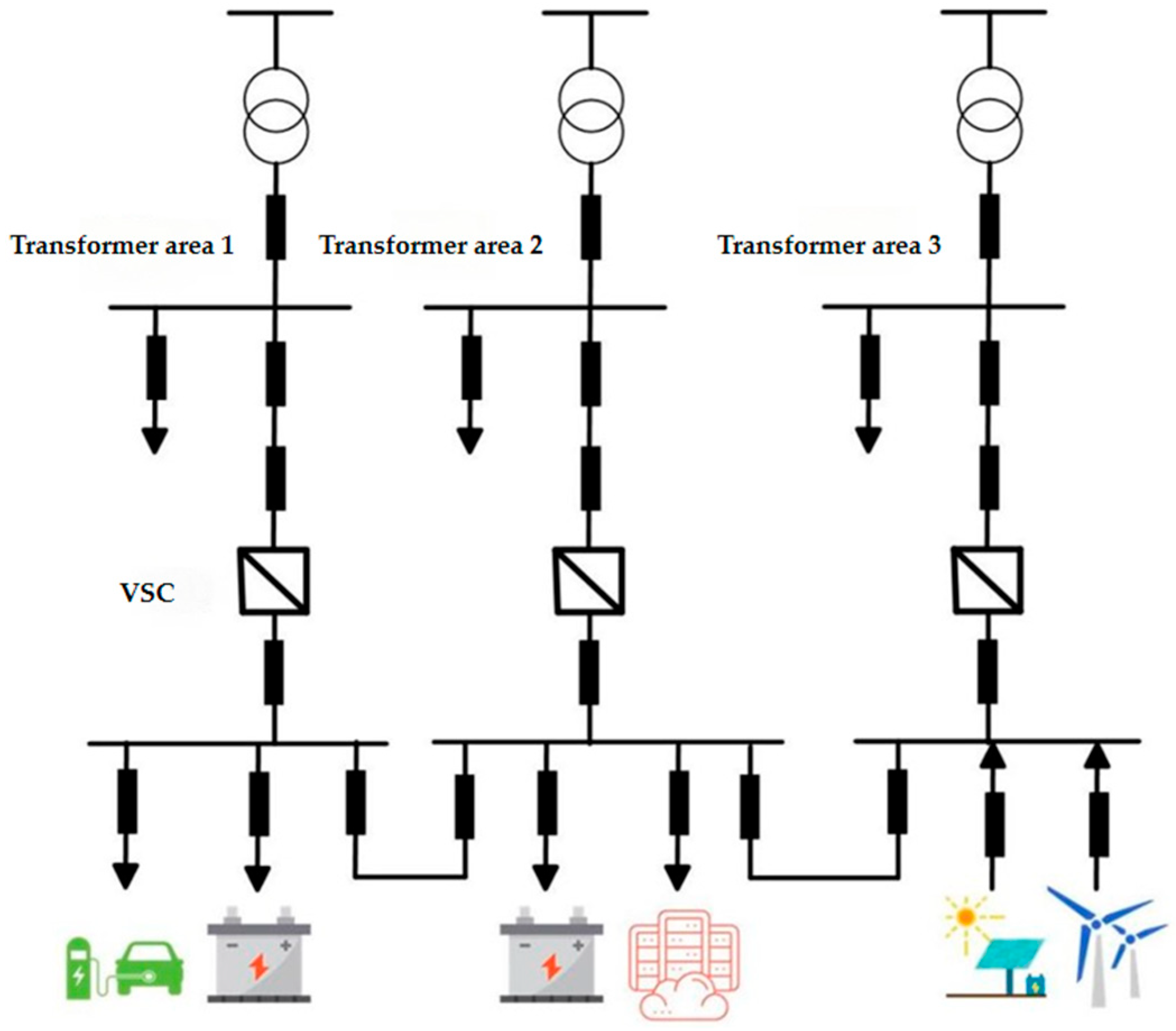
As shown in Figure 1, the hybrid AC/DC flexible interconnection system for distribution transformer areas is applicable to multiple distribution areas with close geographical proximity and predominantly DC loads. Each transformer area is supplied by conventional AC power, while DC power is provided externally through voltage source converters to meet the access requirements of emerging DC loads such as electric vehicle charging stations and data centers [2,16]. In addition, distributed energy resources such as rooftop photovoltaic systems and small-scale wind power generation can also be connected to the DC bus of the system through DC/DC converters. The transformer areas are interconnected via DC tie lines, thereby effectively optimizing power allocation among different transformer areas and improving the overall resource utilization and operational efficiency of the system.

Flexible interconnection technology offers several advantages: by facilitating load sharing between transformer areas, it can effectively improve equipment utilization, reduce system losses, enhance voltage quality, and increase power supply reliability. At the same time, it improves the system’s adaptability to distributed energy resources and promotes flexible power supply scheduling.

However, flexible interconnection systems also face several challenges. First, the system requires high initial investment, especially in the installation of converters and energy storage equipment. Second, flexible interconnection increases the operational complexity of the system, potentially leading to new stability and coordination issues, particularly in large-scale interconnected systems. Additionally, interconnection between transformer areas that are geographically dispersed may result in significant construction and maintenance costs.

3. Interconnection Potential Assessment of Distribution Transformer Areas Based on Load Characteristics

The interconnection potential of transformer areas refers to the capability of adjacent distribution transformer areas, after being interconnected through tie switches or interconnection devices, to realize load transfer, mutual power supply, and operational optimization under security constraints [10]. The load characteristics of distribution transformer areas directly reflect variations in user electricity consumption behavior over time and space and therefore constitute a key basis for assessing interconnection potential. Differences exist among transformer areas in terms of the occurrence time and fluctuation magnitude of load peaks and valleys; if these transformer areas exhibit pronounced complementarity in load time series, flexible interconnection can be utilized to achieve peak shaving and valley filling as well as power mutual support, thereby improving equipment utilization and reducing operational losses. Consequently, conducting interconnection potential assessment based on load characteristics helps to scientifically identify high-potential transformer area combinations with strong load complementarity and reasonable geographical layout, providing a foundation for the subsequent optimal configuration of flexible interconnection systems. In this section, two key indicators in the interconnection potential assessment framework are established, namely the post-interconnection load factor improvement and the geographical dispersion degree of transformer areas, and an interconnection potential assessment procedure for distribution transformer areas is presented to enable the scientific selection of high-potential transformer area combinations.

3.1. Interconnection Potential Assessment Indices for Distribution Transformer Areas

3.1.1. Load Factor Improvement Score

The load factor is defined as the ratio of the average load to the maximum load of a distribution transformer area within a statistical period and is used to characterize the degree of load uniformity. A higher load factor indicates that the average load is closer to the maximum load, resulting in a smoother load curve with less pronounced peak characteristics. After transformer areas are interconnected, loads can be more easily transferred across areas and peak shaving and valley filling can be achieved, thereby improving the feasibility and available operational margin of interconnection operation and leading to greater interconnection potential.

To quantitatively characterize the degree of load uniformity in the load characteristics of distribution transformer areas, this paper adopts the load factor $k_{load}$ as an evaluation index, which is defined as follows:

$$k_{load}={\displaystyle \frac{P_{avg}}{P_{max}}}\times 100\%$$

(1)

where $P_{avg}$ denotes the average load within the statistical period, and $P_{max}$ denotes the maximum load within the same period. To improve clarity, all variables used in the mathematical formulations follow the International System of Units (SI). Power-related variables are expressed in kW, energy-related variables in kWh, costs in CNY or 10⁴ CNY, efficiencies in %, and distances in km unless otherwise specified.

Considering that different transformer area combinations exhibit varying degrees of load factor improvement after interconnection, and that the numerical magnitudes and value ranges of different combinations are not consistent, it is necessary to normalize the load factor improvement to facilitate horizontal comparison among different transformer area combinations and to convert it into a dimensionless score index. Accordingly, the load factor improvement score of transformer area combination $i$ is defined as:

$$S_i^{load}={\displaystyle \frac{\Delta K_i^{load}-\Delta K_{min}^{load}}{\Delta K_{max}^{load}-\Delta K_{min}^{load}}}$$

(2)

where $S_i^{load}$ denotes the load factor improvement score of transformer area combination $i$, $\Delta K_i^{load}$ denotes the load factor improvement of transformer area combination $i$ before and after interconnection, $\Delta K_{min}^{load}$ denotes the minimum load factor improvement among all transformer area combinations after interconnection, and $\Delta K_{max}^{load}$ denotes the maximum load factor improvement among all transformer area combinations after interconnection.

The load factor improvement score is used to measure the degree of load factor improvement of transformer area combinations after interconnection. After interconnection, loads among transformer areas are more reasonably allocated through power mutual support, and the improvement in load factor indicates an increase in equipment capacity utilization efficiency and more efficient system operation. Therefore, the load factor improvement score can be regarded as an important index for evaluating the interconnection benefits of transformer area combinations.

3.1.2. Geographical Dispersion Degree Score

The geographical dispersion degree score reflects the differences in geographical distances among transformer areas. The greater the distance between transformer areas, the higher the construction cost of interconnection; conversely, shorter distances correspond to lower interconnection costs. Therefore, the geographical dispersion degree can be used as a constraint indicator for evaluating the economic performance of interconnection among transformer area combinations.

Similarly, to eliminate the influence of differences in the magnitude and value range of geographical distances among different transformer area combinations, the geographical dispersion degree of transformer area combinations is normalized. Accordingly, the geographical dispersion degree score of transformer area combination $i$ is defined as:

$$S_i^{dis}={\displaystyle \frac{D_i-D_{min}}{D_{max}-D_{min}}}$$

(3)

where $S_i^{dis}$ denotes the geographical dispersion degree score of transformer area combination $i$, $D_i$ denotes the minimum path length connecting all transformer areas within transformer area combination $i$, $D_{min}$ denotes the minimum value of the minimum path lengths among all transformer area combinations, and $D_{max}$ denotes the maximum value of the minimum path lengths among all transformer area combinations.

The geographical dispersion degree score is used to measure the spatial distribution differences among transformer areas within a transformer area combination. A higher score indicates greater geographical distances among transformer areas, longer required interconnection tie lines, and correspondingly higher construction and investment costs; conversely, a lower score indicates a more concentrated spatial distribution of transformer areas and lower interconnection costs. Therefore, the geographical dispersion degree score is negatively correlated with the economic performance of transformer area interconnection and can be used as an important indicator for evaluating the cost constraint of interconnection among transformer area combinations.

It should be noted that this paper uses the straight-line distance between transformer areas as an approximation for the geographical dispersion degree, primarily for quickly comparing the relative construction costs of different transformer area combinations during the planning phase. In urban distribution networks, tie-lines are typically laid along existing roads or corridors, and the straight-line distance can, to some extent, reflect the trend of changes in line length. This study does not further consider complex engineering factors such as road alignment, construction difficulty, and topographical conditions, so this indicator is a simplified approach. A more detailed evaluation of the actual construction costs can be carried out in the subsequent engineering design phase.

3.2. Interconnection Potential Assessment Procedure for Distribution Transformer Areas

In the process of screening transformer area combinations with interconnection potential, the proposed assessment method takes the expected improvement in system load factor after interconnection and the degree of spatial concentration of geographical distribution among transformer areas as two crucial quantitative evaluation dimensions.

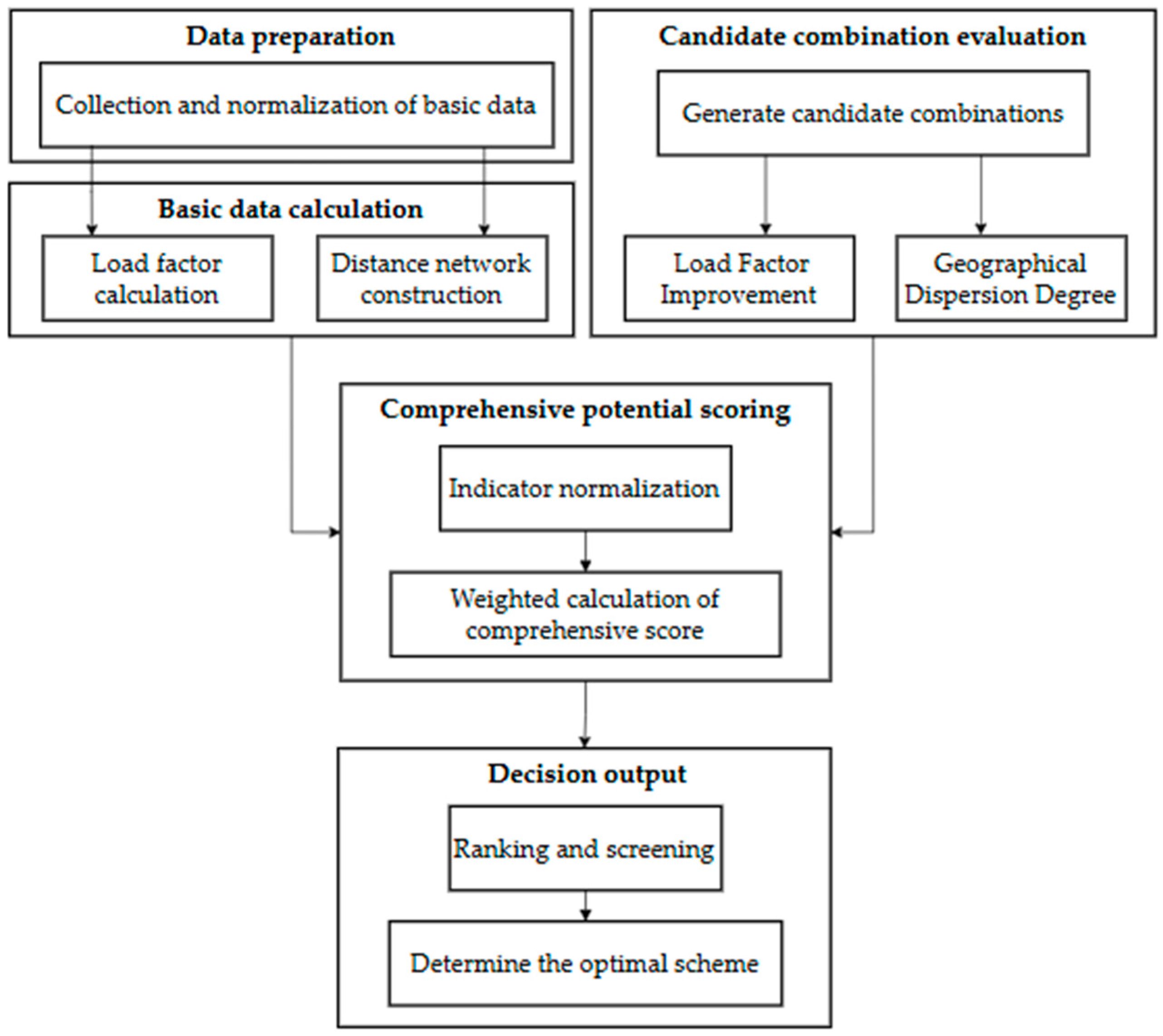
As illustrated in Figure 2, the overall framework of the interconnection potential assessment is presented. The detailed analysis steps are described as follows:

(a)

Collection and normalization of basic data: comprehensively collect the typical-day load data of all distribution transformer areas within the planning scope, and accurately obtain the geographical spatial coordinate information of each transformer area.

(b)

Extraction of characteristic parameters of individual transformer areas and construction of the distance network: analyze the load data of each transformer area and calculate its load factor $k_i^{load}$. Based on the geographical spatial coordinates of each transformer area, calculate and construct a distance network dataset that contains the straight-line distance information $d_{i,j}$ between all pairs of transformer areas.

$$k_i^{load}={\displaystyle \frac{P_{i.avg}}{P_{i.max}}}$$

(4)

$$d_{i,j}=\sqrt{{\left(x_i-x_j\right)}^2+{\left(y_i-y_j\right)}^2}$$

(5)

where $k_i^{load}$ denotes the load factor of transformer area $i$, $P_{i.avg}$ denotes the average load of transformer area $i$ within the statistical period, $P_{i.max}$ denotes the maximum load of transformer area $i$ within the statistical period, $d_{i,j}$ denotes the straight-line distance between transformer area $i$ and transformer area j, and ($x_i$, $y_i$) represents the location coordinates of transformer area $i$.

(c)

Generation of candidate interconnection combinations and calculation of post-interconnection load characteristics: to effectively explore the benefits brought by interconnection among small-scale clusters of transformer areas, the number of interconnected transformer areas is set to $n$. All possible and non-redundant transformer area combinations are generated, and for each generated combination, the theoretical maximum load factor after interconnection, $K_i^{load}$, is calculated.

It should be noted that the “theoretical maximum load factor after interconnection” defined in this paper is primarily used as an upper bound estimate of potential during the planning stage. In the calculation process, only the optimal load redistribution under the power conservation condition between transformer areas is considered, without introducing specific operational constraints such as converter capacity, tie-line capacity, or transformer rated capacity. This indicator aims to characterize the load balancing potential of different transformer area combinations under ideal complementary conditions, and is used for relative comparison between candidate combinations. Actual operational constraints will be incorporated into the subsequent optimization configuration model.

(d)

Quantification of interconnection benefit indicators and geographical cost indicators: for each transformer area combination, it is necessary to quantitatively evaluate its potential interconnection benefits. First, the load factor of each transformer area within the combination under independent operation is calculated, and their average value $K_{i.avg}^{load}$ is obtained, i.e.,

$$K_{i.avg}^{load}={\displaystyle \frac{{\displaystyle \sum k_i^{load}}}{n}}$$

(6)

where $K_{i.avg}^{load}$ denotes the average load factor of all transformer areas in transformer area combination $i$ under independent operation, and ${\displaystyle \sum k_i^{load}}$ denotes the sum of the load factors of the $n$ transformer areas in transformer area combination $i$ under independent operation.

Then, the theoretical maximum load factor after interconnection of the transformer area combination is compared with the above average load factor under independent operation, and the difference between the two is regarded as the load factor improvement, denoted as $\Delta K_i^{load}$, i.e.,

$$\Delta K_i^{load}=K_i^{load}-K_{i.avg}^{load}$$

(7)

where $\Delta K_i^{load}$ denotes the load factor improvement of transformer area combination $i$ before and after interconnection, and $K_i^{load}$ denotes the theoretical maximum load factor of transformer area combination $i$ after interconnection.

This value directly reflects the degree of improvement in equipment utilization efficiency brought about by the complementary effect of loads. Meanwhile, based on the previously constructed distance network data, the geographical distances between every pair of transformer areas within the transformer area combination are extracted, and the minimum path length connecting all transformer areas in the combination, denoted as $D_i$, is obtained as the core indicator for measuring the geographical dispersion degree of the combination. To a certain extent, this minimum distance value represents the maximum potential connection cost required for constructing the interconnection network.

(e)

Normalization of evaluation indicators: to eliminate the influence of differences in physical meaning and numerical variation ranges among different evaluation indicators on the final assessment results, the load factor improvement and the minimum distance value obtained in Step (4) are normalized, yielding the load factor improvement score $S_i^{load}$ and the geographical dispersion degree score $S_i^{dis}$ of transformer area combination $i$.

(f)

Construction of the comprehensive interconnection potential scoring model: to comprehensively balance the improvement of load utilization benefits and the control of geographical connection costs, predefined weight coefficients ${\alpha }_c$ and ${\beta }_c$ are assigned to the load factor improvement score and the geographical dispersion degree score, respectively, and the comprehensive score $S_i^{Total}$ is calculated, i.e.,

$$S_i^{Total}=S_i^{load}\cdot {\alpha }_c+S_i^{dis}\cdot {\beta }_c$$

(8)

where $S_i^{Total}$ denotes the comprehensive score of transformer area combination $i$. Through the comprehensive score, the interconnection potential of each transformer area combination is quantitatively evaluated.

(g)

Ranking of candidate combinations and final selection: based on the interconnection potential of each transformer area combination calculated in the previous steps, all combinations are ranked in descending order. The combination with the highest score is identified as the candidate scheme with the greatest interconnection potential. After rigorous screening and evaluation, the selected transformer area combinations are selected for further detailed and in-depth studies, including flexible interconnection system design, comprehensive economic assessment, and specific technical feasibility analysis.

Through the above series of analysis procedures, the proposed quantitative interconnection potential assessment method can scientifically and quantitatively screen out interconnection schemes with the greatest practical application value from a large number of potential transformer area combinations, thereby providing critical decision-support information for the upgrading and intelligent development of modern distribution networks.

Interconnection potential assessment provides theoretical support and directional guidance for transformer area interconnection. However, it is still necessary to further comprehensively consider operational constraints such as capacity limits, voltage constraints, and equipment selection, as well as equipment configuration costs. Therefore, this paper establishes an optimal configuration model for the flexible interconnection system of distribution transformer areas to conduct further research.

4. Optimal Configuration Model for the Flexible Interconnection System of Distribution Transformer Areas

This study is dedicated to developing an optimal configuration model for the flexible interconnection system of distribution transformer areas, with the core objective of minimizing the annualized total system cost. The total cost function comprehensively considers capital asset investment and energy losses during system operation. By optimally configuring the capacity parameters of the key equipment in each transformer area within the interconnection system, the proposed model aims to achieve a balanced solution between economic benefits and technical performance, enhance the power supply reliability and power quality of regional distribution networks, and strengthen the local accommodation and efficient utilization of intermittent distributed generation.

4.1. Objective Function

The objective of the optimal configuration of the flexible interconnection system for distribution transformer areas is to minimize the total investment and operation cost of the interconnection system, i.e.,

$$C=\min \left(C_{in}+C_{op}\right)$$

(9)

where $C$ denotes the total cost of the optimal configuration model for the flexible interconnection of transformer areas, $C_{in}$ denotes the capital investment cost, and $C_{op}$ denotes the operation cost.

The capital investment cost $C_{in}^{VSC}$ includes the investment cost of grid-connected converters $C_{in}^{VSC}$ and the investment cost of energy storage units $C_{in}^{bat}$, where the investment of energy storage units is further divided into the investment in energy storage batteries and the investment in DC/DC interfaces [23], i.e.,

$$C_{in}=\beta \left(C_{in}^{VSC}+C_{in}^{bat}\right)$$

(10)

$$C_{in}^{VSC}=c_{in}^{VSC}{\displaystyle \sum _{i=1}^n{Q}_{i.max}^{VSC}}$$

(11)

$$C_{in}^{bat}=c_{in}^{DC}{\displaystyle \sum _{i=1}^n{Q}_{i.max}^{DC}}+c_{in}^{bat}{\displaystyle \sum _{i=1}^n{Q}_{i.max}^{bat}}$$

(12)

$$\beta ={\displaystyle \frac{\lambda {\left(1+\lambda \right)}^{\alpha }}{{\left(1+\lambda \right)}^{\alpha }-1}}$$

(13)

where $\beta$ is the capital recovery factor, the purpose of $\beta$ is to convert the initial capital investment into an equivalent annual cost, taking into account the interest rate and the service life of the equipment. This factor helps balance the upfront investment with the ongoing operational costs, making it a key parameter in evaluating the economic feasibility of the system. $\lambda$ is the annual interest rate, and $\alpha$ is the service life of the equipment. $C_{in}^{VSC}$, $c_{in}^{DC}$, and $c_{in}^{bat}$ denote the unit capacity investment costs of the converter, DC/DC interface, and energy storage battery, respectively. $n$ denotes the number of transformer areas; $Q_{i.max}^{VSC}$ denotes the rated capacity of the converter in transformer area $i$; $Q_{i.max}^{DC}$ denotes the rated capacity of the DC/DC interface of the energy storage unit in transformer area $i$; and $Q_{i.max}^{bat}$ denotes the energy storage battery capacity of transformer area $i$.

The system’s annual operating cost consists of three components: transformer operating costs, converter operating costs, and energy storage unit operating costs. These costs mainly arise from the energy losses during the operation of each device. The low-voltage supply radius is generally not recommended to exceed 300 m and based on related demonstration projects, it is known that the interconnecting transformer areas are geographically close, with short tie-line lengths [24]. The power transmission loss from the tie-lines typically accounts for no more than 1% to 2% of the total system losses. Therefore, for short interconnection tie-lines on the order of a few hundred meters, the associated power loss is expected to be relatively low and can be reasonably neglected in the context of capacity and cost optimization. Therefore, the power transmission losses caused by the tie-lines are not considered in this model, i.e.,

$$C_{op}=C_{op}^{tran}+C_{op}^{VSC}+C_{op}^{bat}$$

(14)

The transformer operation cost corresponds to the transformer energy loss, which mainly includes iron loss and copper loss, i.e.,

$$C_{op}^{tran}=c_{cost}\left(C^{Fe}+C^{Cu}\right)$$

(15)

$$C^{Fe}={\displaystyle \sum _{t=1}^T{\displaystyle \sum _{i=1}^n{P}_i^{Fe}\Delta t}}={\displaystyle \sum _{t=1}^T{\displaystyle \sum _{i=1}^n(k_1{S}_{N.i}^{tran}+b_1)\Delta t}}$$

(16)

$$C^{Cu}={\displaystyle \sum _{t=1}^T{\displaystyle \sum _{i=1}^n{P}_i^{Cu}{\left({\gamma }_{i.t}^{tran}\right)}^2\Delta t}}={\displaystyle \sum _{t=1}^T{\displaystyle \sum _{i=1}^n\left(k_2{S}_{N.i}^{tran}+b_2\right){\left({\gamma }_{i.t}^{tran}\right)}^2\Delta t}}$$

(17)

$${\gamma }_{i.t}^{tran}={\displaystyle \frac{P_{i.t}^{tran}}{S_{N.i}^{tran}\cos \theta }}$$

(18)

where $c_{cost}$ denotes the electricity price; $S_{N.i}^{tran}$ denotes the rated capacity of the transformer in transformer area $i$; $T$ denotes the total number of time periods; and $\Delta t$ denotes the length of each time period. $P_i^{Fe}$ denotes the iron loss of the transformer in transformer area $i$, and $P_i^{Cu}$ denotes the rated copper loss of the transformer. ${\gamma }_{i.t}^{tran}$ denotes the transformer loading ratio. In practical engineering applications, the rated copper loss and iron loss of transformers are usually linearly related to the transformer capacity, where $k_1$, $k_2$, $b_1$, $b_2$ are linear fitting parameters. $P_{i.t}^{tran}$ denotes the active power flowing through the transformer, with the positive direction defined from the high-voltage side to the low-voltage side, and $\cos \theta$ denotes the power factor.

If the total transformer losses in the interconnection model are minimized, i.e., the ideal load allocation state is achieved, the transformer loading ratios of each transformer area satisfy:

$${\gamma }_i^{tran}:{\gamma }_j^{tran}={\displaystyle \frac{S_{N.i}^{tran}}{P_i^{Cu}}}:{\displaystyle \frac{S_{N.j}^{tran}}{P_j^{Cu}}}$$

(19)

It is assumed that the transformers in each transformer area are of the same model. This assumption helps to highlight the impact of flexible interconnection on load redistribution and equipment utilization improvement. In practical engineering applications, if there are differences in transformer capacity or loss parameters, the optimal load distribution result will be related to the capacity and loss characteristics. However, the model structure and solution method remain applicable. When the load factors of all transformers are equal, the total power consumption of the transformers within the interconnection model is minimized.

The converter operation cost depends on the power transmission loss of the converter, i.e.,

$$C_{op}^{VSC}=c_{cost}{\displaystyle \sum _{t=1}^T{\displaystyle \sum _{i=1}^n{P}_{i.t}^{VSC}\left(1-{\epsilon }_i^{VSC}\right)\Delta t}}$$

(20)

where $P_{i.t}^{VSC}$ denotes the AC-side active power of the converter in transformer area $i$ at time period $t$, with the positive direction defined from the AC side to the DC side; and ${\epsilon }_i^{VSC}$ denotes the converter efficiency.

The operation cost of the energy storage unit is composed of the transmission loss of the DC/DC interface [15], i.e.,

$$C_{op}^{bat}=c_{cost}{\displaystyle \sum _{t=1}^T{\displaystyle \sum _{i=1}^n(P_{i.t}^{ch}+P_{i.t}^{dis})\left(1-{\epsilon }_i^{bat}\right)\Delta t}}$$

(21)

where $P_{i.t}^{ch}$ denotes the charging power of the energy storage unit in transformer area $i$ at time period $t$, $P_{i.t}^{dis}$ denotes the discharging power of the energy storage unit and ${\epsilon }_i^{bat}$ denotes the DC/DC interface efficiency of the energy storage unit.

The decision variables of the optimal configuration model for flexible interconnection include the rated capacity of converters $Q_{i.max}^{VSC}$, the rated capacity of the DC/DC interface of energy storage units $Q_{i.max}^{DC}$, the energy storage battery capacity $Q_{i.max}^{bat}$, the operational state variable of energy storage units $F_i^{bat}(t)$, the charging power $P_{i.t}^{ch}$, the discharging power $P_{i.t}^{dis}$, and the transmission power of interconnection tie lines $P_{i.t}^{line}$.

4.2. Constraints

AC-side active power balance constraint of transformer areas:

$$P_{i.t}^{tran}=P_{i.t}^{VSC}+P_{i.t}^{AC}$$

(22)

where $P_{i.t}^{AC}$ denotes the AC load of transformer area $i$ at time period $t$.

DC-side active power balance constraint of transformer areas:

$$P_{i.t}^{VSC}{\epsilon }_i^{VSC}+P_{i.t}^{DG}=P_{i.t}^{DC}-P_{i.t}^{dis}+P_{i.t}^{line}$$

(23)

where $P_{i.t}^{DG}$ denotes the output power of distributed generation, $P_{i.t}^{DC}$ denotes the DC load, and $P_{i.t}^{line}$ denotes the interconnection line transmission power.

Energy balance constraint of energy storage units:

$${\epsilon }_i^{bat}{\displaystyle \sum _{t=1}^{24}{P}_{i.t}^{ch}}={\displaystyle \frac{1}{{\epsilon }_i^{bat}}}{\displaystyle \sum _{t=1}^{24}{P}_{i.t}^{dis}}$$

(24)

Transformer power constraint:

$$\left|{\gamma }_{i.t}^{tran}\right|\le {\gamma }_{max}^{tran}$$

(25)

where ${\gamma }_{max}^{tran}$ denotes the upper limit of the transformer loading ratio.

Converter power constraint:

$$\left|P_{i.t}^{VSC}\right|\le Q_{i.max}^{VSC}$$

(26)

Power constraint of the DC/DC interface of energy storage units:

$$0\le P_{i.t}^{ch}\le F_i^{bat}(t)Q_{i.max}^{DC}$$

(27)

$$0\le P_{i.t}^{dis}\le \left(1-F_i^{bat}\left(t\right)\right)Q_{i.max}^{DC}$$

(28)

State-of-charge constraint of energy storage batteries:

$$Q_i^{bat}\left(t\right)\in \left[Q_{i.min}^{bat},Q_{i.max}^{bat}\right]$$

(29)

$$Q_i^{bat}\left(t\right)={\displaystyle \frac{1}{Q_{i.max}^{bat}}}\left(Q_i^{bat}\left(0\right)+{\epsilon }_i^{bat}{\displaystyle \sum _{t=1}^{24}{P}_{i.t}^{ch}}\Delta t-{\displaystyle \frac{1}{{\epsilon }_i^{bat}}}{\displaystyle \sum _{t=1}^{24}{P}_{i.t}^{dis}\Delta t}\right)$$

(30)

where $Q_i^{bat}\left(t\right)$ denotes the state of charge of the energy storage battery in transformer area $i$ at time $t$, $Q_{i.min}^{bat}$ and $Q_{i.max}^{bat}$ denote the lower and upper limits of the state of charge, respectively, and $Q_i^{bat}\left(0\right)$ denotes the initial energy of the energy storage battery.

Cycle life constraint of energy storage batteries [15]:

$${\displaystyle \sum _{t=1}^T{X}_i^{bat}\left(t\right)}\le X_{life.i}^{bat}$$

(31)

$$X_i^{bat}\left(t\right)=\max \left(F_i^{bat}\left(t\right)-F_i^{bat}\left(t-1\right),0\right)$$

(32)

where $X_i^{bat}\left(t\right)$ denotes the cycle counting variable of the energy storage battery; it takes the value of 1 when the energy storage battery in transformer area $i$ starts charging at time t, and 0 otherwise. $X_{life.i}^{bat}$ denotes the cycle life of the energy storage battery, and $F_i^{bat}\left(t\right)$ denotes the operational state variable of the energy storage unit, which takes the value of 0 when the energy storage unit is not in operation.

This study uses a linear fitting method based on the indicators of load evaluation and combines it with mixed integer linear programming (MILP) optimization, where the model includes 0–1 variables such as energy storage operating state variables and cycle count variables. Both the objective function and constraints can be linearized, and the optimization model is solved using the CPLEX solver on the MATLAB R2023a platform.

5. Case Samples and Parameter Settings

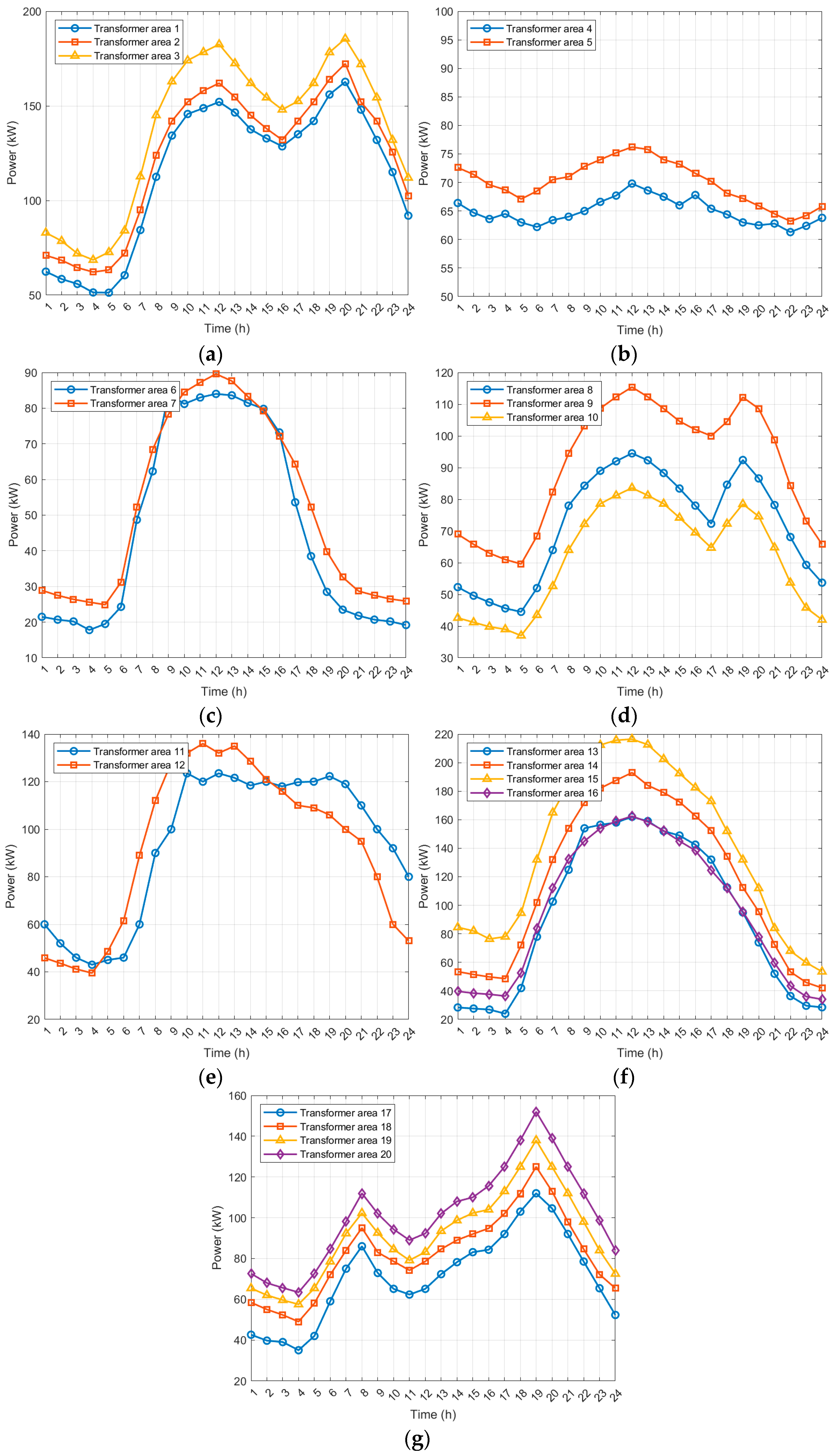
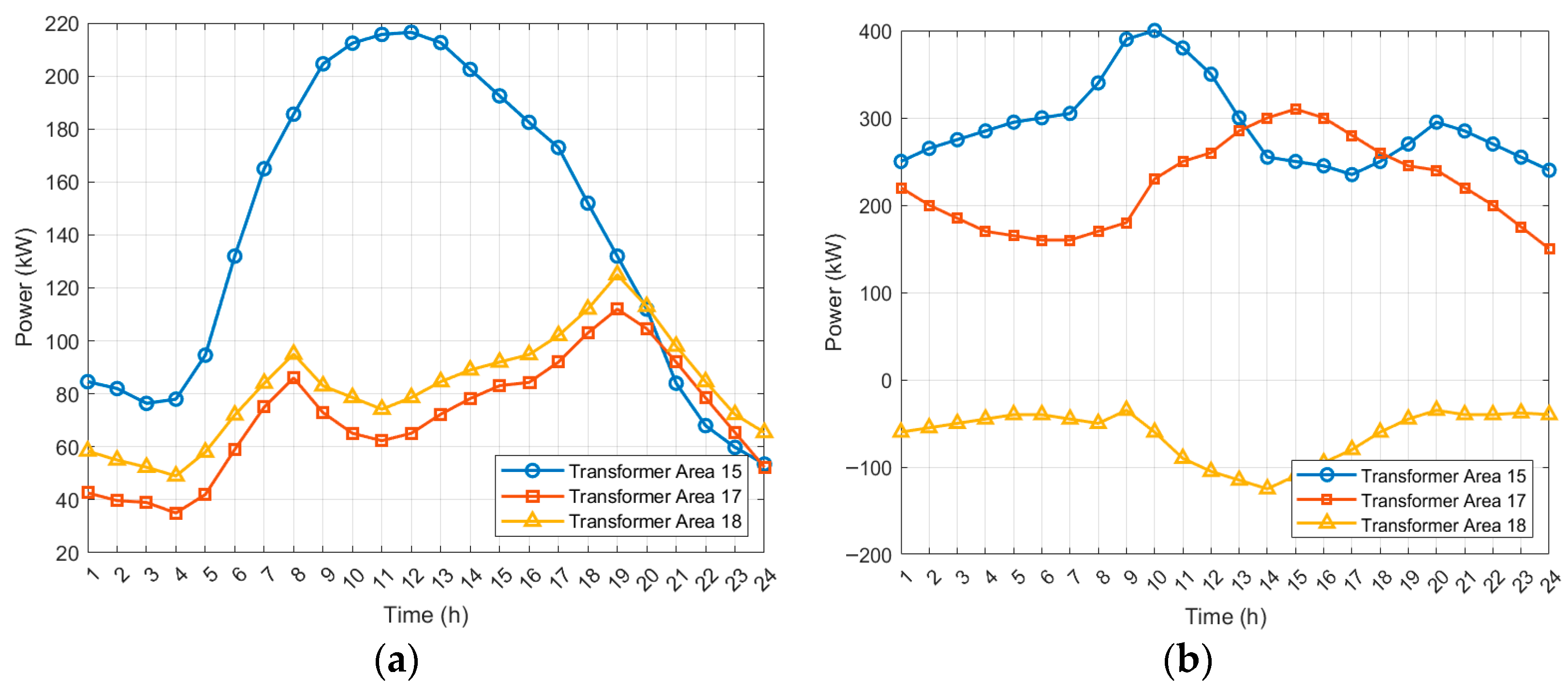
To ensure the diversity and representativeness of the research samples, this paper selects 20 distribution transformer areas from a typical urban region in a city in Henan Province as case study samples, covering multiple typical electricity consumption scenarios such as commercial, medical, governmental, residential, educational, and industrial loads. The load curves of different types of transformer areas on a typical day are shown in Figure 3. Specifically, transformer areas No. 1–3 are commercial areas; No. 4 and No. 5 are hospitals; No. 6 and No. 7 are governmental office areas; No. 8–10 are hotels; No. 11 and No. 12 are university campuses; No. 13–16 are industrial areas; and No. 17–20 are residential areas. Additionally, this paper analyzes using typical 24-h daily load data, with a time resolution of 1 h, T = 24.

Figure 3 illustrates the load curves of different transformer areas over a 24-h period. These curves show the variation in power demand throughout the day, highlighting both peak and off-peak load periods. The load curves represent typical profiles for residential, commercial, and industrial sectors. Residential loads typically exhibit peak demand during the morning and evening, while commercial and industrial loads may have more varied demand patterns depending on operating hours. These specific load profiles were selected to demonstrate the differing temporal characteristics of power consumption across various sectors, which are crucial for assessing the interconnection potential and optimizing load distribution strategies in the distribution network.

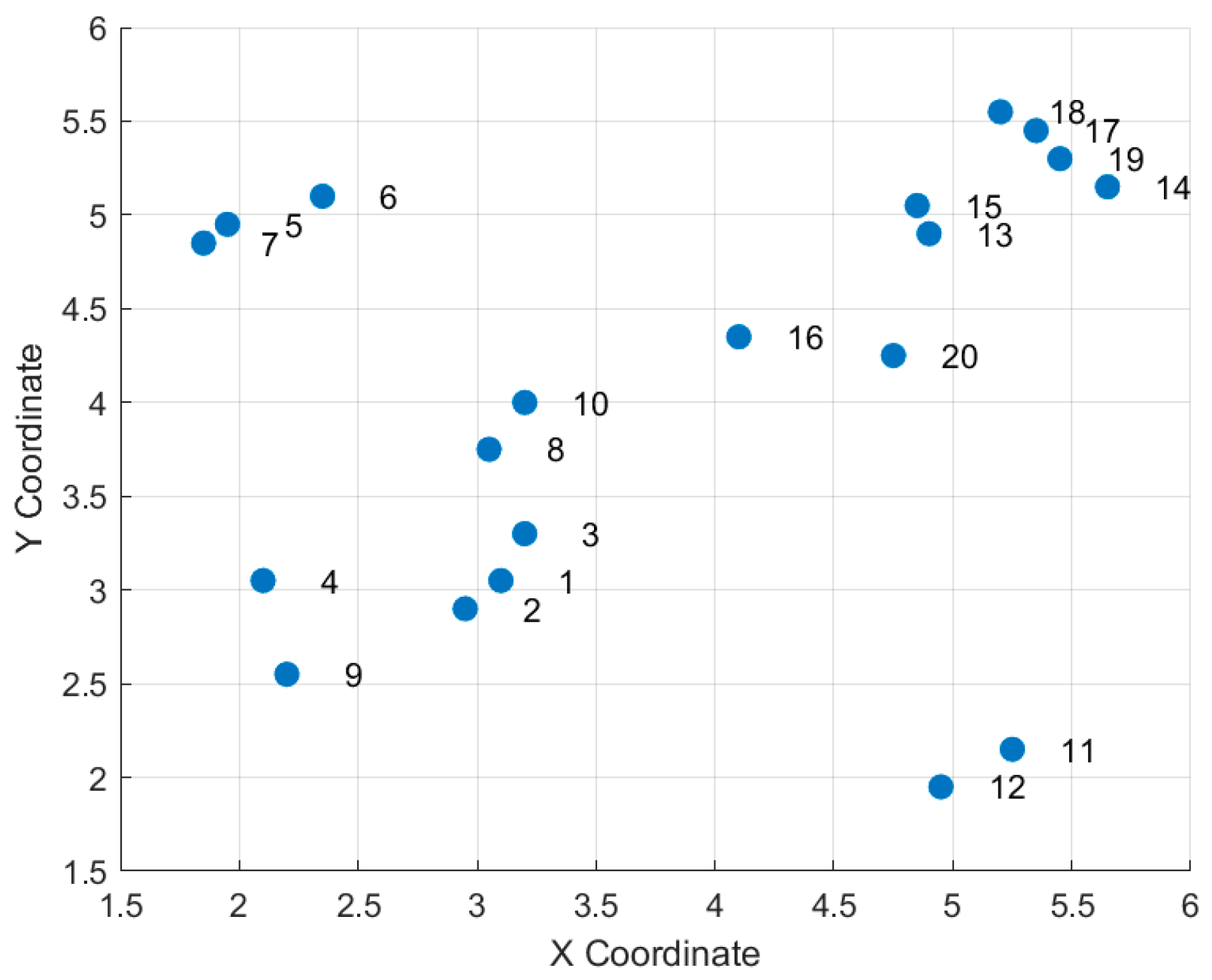
The geographical distribution of the 20 transformer areas is shown in Figure 4.

In this case study, the number of interconnected transformer areas is set to 3. The interconnection scale is determined by considering both load complementarity effects and the complexity of engineering implementation. In urban distribution networks, flexible interconnection is typically carried out with a small number of adjacent transformer areas as the basic unit. A three-area interconnection can reflect the multi-source load complementarity and power coordination characteristics, while maintaining a relatively simple structure. If only two transformer areas are interconnected, the complementarity dimension is limited; further expanding the interconnection scale would significantly increase the number of combinations and the complexity of the system structure. Therefore, this study selects the three-area interconnection as a representative research scale.

The weight coefficients for load rate improvement and geographical dispersion degree scores are set to 0.7 and −0.3, respectively. These weight coefficients reflect the focus of the planning phase. Since the core objective of flexible interconnection is to improve operational efficiency, the weight of the load rate improvement indicator is appropriately increased, while the geographical dispersion degree serves to constrain construction costs. Thus, the weight settings balance operational efficiency and engineering feasibility. In practical applications, the weight coefficients can be flexibly adjusted according to planning goals and investment preferences.

By analyzing combinations of 20 distribution transformer areas, a comprehensive evaluation is conducted based on their performance in both load rate improvement potential and geographical dispersion degree.

In the subsequent optimal configuration, the annual interest rate is set to 0.08, the equipment service life is set to 10 years, and the average electricity price is 0.636 CNY/kWh. Considering that the distribution system in the case study is mainly integrated with electric vehicle fast-charging stations and distributed generation, the power factor of the distribution transformer areas is set to 0.95. According to the literature [25,26], the relevant investment costs of distribution equipment are determined based on practical engineering experience. Specifically, these investment costs take into account factors such as the design, manufacturing, installation, and maintenance of the equipment, and play an important role in equipment selection and system economic analysis.

Table 3. Parameters for the case study.

Equipment Type	Parameter	Value
Transformer	Linear fitting parameter $a$	0.0012
	Linear fitting parameter $b$	0.0077
	Linear fitting parameter $c$	0.0091
	Linear fitting parameter $d$	0.61
	Maximum load factor (%)	80
Converter	Unit capacity investment cost (CNY/kW)	2000
	Converter efficiency (%)	98
Energy storage unit	Unit capacity investment cost of DC/DC interface (CNY/kW)	500
	Unit capacity investment cost of battery (CNY/kW)	500
	DC/DC interface efficiency (%)	99
	Upper limit of state of charge (%)	100
	Lower limit of state of charge (%)	20
	Charge–discharge cycle life (cycles)	5000

lists the key investment cost parameters for each type of equipment.

The distribution transformers used in this study have a rated capacity of 10 MVA, which is typical for medium-voltage distribution networks. They have an impedance of 6%, standard for transformers of this size, and operate with primary voltage of 10 kV and secondary voltage of 0.4 kV. The no-load losses are 0.5% of the rated capacity, with load losses calculated based on the actual load factor. The transformers are oil-immersed, which ensures optimal performance and thermal stability during operation in urban distribution networks. These technical characteristics align with industry standards and are representative of typical configurations used in distribution networks.

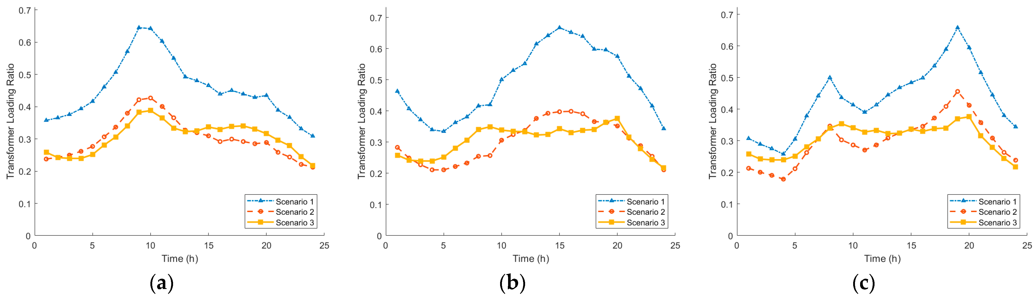
To evaluate the comprehensive effectiveness of the proposed flexible interconnection optimal configuration model in improving equipment capacity utilization efficiency, promoting the local accommodation of distributed renewable energy, and reducing the system life-cycle economic cost, three scenarios are designed in this case study, as described below:

Scenario 1: The three transformer areas operate independently. Each transformer area satisfies the hybrid AC/DC power supply demand through an AC/DC converter, and no energy storage unit is installed in any transformer area.

Scenario 2: The three transformer areas operate independently. Each transformer area satisfies the hybrid AC/DC power supply demand through an AC/DC converter, and energy storage units are installed in all transformer areas.

Scenario 3: The three transformer areas operate in an interconnected manner, and energy storage units are installed in all transformer areas.

6. Comparative Analysis of Case Study Results

6.1. Comparative Analysis of Interconnection Potential Assessment Results

Based on the transformer area interconnection potential assessment method proposed in Section 3, the interconnection potential of all candidate transformer area combinations is calculated and ranked. It should be noted that if the number of transformer areas in the planning region is N and the interconnection scale is n, the number of candidate combinations is C(N, n). In this case study (N = 20, n = 3), the number of combinations is 1140, which is relatively small and can be completed offline during the planning phase. When the number of transformer areas increases, the number of combinations grows combinatorially with N. For large-scale systems, the candidate range can be narrowed through preliminary clustering based on load characteristics or by using partitioned hierarchical assessments, effectively reducing the computational complexity.

Among them, the top five transformer area combinations with the highest interconnection potential are listed in

Table 4. Comparison of indicators for the top five transformer area combinations.

Rank	Transformer Area Combination	Average Load Factor Before Interconnection (%)	Load Factor After Interconnection (%)	Load Factor Improvement Score	Geographical Dispersion Degree Score	Total Score
1	15–17–18	64.6	79.4	1.000	0.052	0.684
2	15–17–19	64.8	79.2	0.980	0.051	0.670
3	14–17–18	63.2	77.2	0.961	0.058	0.655
4	14–17–19	63.3	77.0	0.953	0.041	0.655
5	15–17–20	64.9	78.9	0.954	0.061	0.650

. It can be observed that the transformer area combination with the greatest interconnection potential is 15–17–18. The geographical dispersion degree score of this combination is 0.052, and the load factor improvement score is 1. After simulated interconnection, the load factor increases from 64.6% to 79.4%, with an improvement rate of 22.9%.

To demonstrate the robustness of the proposed method, a sensitivity analysis was conducted by varying the weight coefficient of the load factor. Specifically, the weight was adjusted from 0.7 to 0.6, and the ranking of the candidate interconnection combinations was observed. The results are shown in

Table 5. Sensitivity analysis of interconnection candidate combinations with varying load factor weights.

Weight	Rank	Transformer Area Combination	Average Load Factor Before Interconnection (%)	Load Factor After Interconnection (%)	Max Distance	Average Distance	Total Score
0.7/−0.3	1	15–17–18	64.6	79.4	0.64	0.47	0.684
	2	15–17–19	64.8	79.2	0.65	0.49	0.670
	3	14–17–18	63.2	77.2	0.60	0.40	0.655
	4	14–17–19	63.3	77.0	0.42	0.28	0.655
	5	15–17–20	64.9	78.9	0.65	0.55	0.650
0.6/−0.4	1	15–17–18	64.6	79.4	0.64	0.47	0.571
	2	14–17–19	63.3	77.0	0.42	0.28	0.562
	3	15–17–19	64.8	79.2	0.65	0.49	0.561
	4	14–17–18	63.2	77.2	0.60	0.40	0.555
	5	15–18–19	65.5	79.4	0.65	0.53	0.546

, where it can be seen that the overall ranking of the candidate combinations remains stable despite the slight change in weight.

As shown in Table 5, the ranking of the candidate combinations does not significantly change with a decrease in the load factor weight. This confirms that the method is robust and the ranking results are stable under different weight settings.

In the subsequent optimal configuration, the transformer area combination 15–17–18 with the highest comprehensive score is selected. The typical daily AC load curves and DC load curves of each transformer area are shown in Figure 5.

6.2. Comparison of Load Factors of Transformer Area Combinations Under Different Scenarios

Based on the results of the interconnection potential assessment, the transformer area combination 15–17–18 with the highest comprehensive score is selected as the research object. A comparative analysis of the load factor performance under three typical operating scenarios is conducted. The load factor results of each transformer area under different scenarios are shown in

Table 6. Load factors of transformer areas under different scenarios.

Transformer Area	Load Factor in Scenario 1 (%)	Load Factor in Scenario 2 (%)	Load Factor in Scenario 3 (%)
15	70.52	70.80	79.19
17	73.74	75.45	80.05
18	65.69	65.69	80.04

.

As shown in Table 6, in Scenario 1, the load factors of transformer areas 15, 17, and 18 are 70.52%, 73.74%, and 65.69%, respectively. In Scenario 2, after deploying local energy storage, the load factors of transformer areas 15 and 17 increase to 70.80% and 75.45%, respectively, while the load factor of transformer area 18 remains unchanged. In Scenario 3, the load factors of all three transformer areas are significantly improved, reaching 79.19%, 80.05%, and 80.04%, respectively. These results indicate that flexible interconnection breaks the “islanded” boundaries caused by independent operation among transformer areas. Through cross-area power sharing, the temporal complementary characteristics of loads are fully exploited, enabling the peak load of a single transformer area to be jointly shared by other transformer areas during off-peak periods, thereby effectively suppressing peak demand. Consequently, the overall system load curve becomes smoother, and the load factors are improved and converge to a similar level of approximately 80%, demonstrating a significant enhancement in the operational efficiency of the interconnection system.

To more intuitively illustrate the effects of transformer area interconnection under the three scenarios on improving load curves and enhancing equipment utilization, the transformer loading ratios after interconnection are calculated and compared with those before interconnection. The results are shown in Figure 6.

As shown in Figure 6, compared with the independent operation scenario, the overall level of transformer loading ratios in each transformer area is significantly increased after interconnection, while the intra-day fluctuation amplitude is noticeably reduced. The load factor curves become smoother and more consistent, indicating that flexible interconnection can effectively realize peak shaving and load balancing through cross-area power sharing, thereby improving equipment capacity utilization efficiency and enhancing system operating conditions. Meanwhile, the load factors of different transformer areas gradually converge to a similar level after interconnection, demonstrating that the overall load allocation of the system becomes more balanced and the complementary characteristics of loads among transformer areas are fully exploited. These results further verify that the flexible interconnection scheme can effectively alleviate the power supply pressure of some transformer areas during peak periods and improve the operational stability and economic performance of the interconnection system.

6.3. Comparative Analysis of Optimal Configuration Results of the Distribution System

The total economic cost and its composition under different scenarios are shown in

Table 7. Total economic cost and its composition under different scenarios.

Scenario	Capital Investment Cost (104 CNY)	Operating Cost (104 CNY)	Total Economic Cost (104 CNY)
1	15.69	14.83	30.52
2	16.18	8.62	24.80
3	12.57	7.22	19.79

. As can be seen from Table 7, there are significant differences in the system economic cost among the three operating scenarios. In Scenario 1, each transformer area operates independently without energy storage, resulting in limited load regulation capability during system operation and relatively large operating losses, which lead to high operating costs and a high total economic cost. In Scenario 2, energy storage systems are deployed on the basis of independent operation. Although the capital investment cost increases, energy storage plays a positive role in peak shaving and load balancing, significantly reducing the operating cost and consequently lowering the total system economic cost. In contrast, Scenario 3 achieves power sharing and resource coordination among transformer areas through flexible interconnection. While further reducing operating costs, the optimal capacity configuration at the system level effectively decreases the demand for capital investment, resulting in the lowest total economic cost and the best overall economic performance.

The converter capacities of each transformer area under different scenarios are shown in

Table 8. Converter capacities of transformer areas under different scenarios.

Scenario	Converter Capacity of Transformer Area 15 (kW)	Converter Capacity of Transformer Area 17 (kW)	Converter Capacity of Transformer Area 18 (kW)
1	408.2	316.3	5.0
2	398.0	306.1	5.0
3	330.8	178.1	36.6

. As can be seen from Table 8, in Scenarios 1 and 2, each transformer area mainly operates independently, and the converter capacity is primarily determined by the local DC load peak and the output of distributed generation. Therefore, even after deploying energy storage, the converter capacity only exhibits a slight reduction and remains at a relatively high level overall. In contrast, under the flexible interconnection operating mode in Scenario 3, each transformer area can realize cross-area power sharing through tie lines, allowing part of the power demand during peak periods to be shared by other transformer areas. As a result, local peak power demand is effectively reduced, leading to an overall downward trend in converter capacity configuration. This indicates that flexible interconnection at the system level can alleviate the power pressure of individual transformer areas, reduce the required converter capacity, and improve the rationality and economic efficiency of equipment configuration.

The energy storage capacities of each transformer area under different scenarios are shown in

Table 9. Energy storage capacities of transformer areas under different scenarios.

Scenario	DC/DC Interface Capacity (kW)			Battery Capacity (kWh)
	Transformer Area 15	Transformer Area 17	Transformer Area 18	Transformer Area 15	Transformer Area 17	Transformer Area 18
1	0	0	0	0	0	0
2	12.5	12.5	1.0	15.0	15.0	5.0
3	2.3	2.3	2.3	5.0	5.0	5.0

. As can be seen from Table 9, in Scenario 2, each transformer area is equipped with an energy storage system of a certain scale under independent operation conditions to achieve local peak shaving and load balancing. As a result, the energy storage capacity configuration exhibits a scattered and uneven distribution, with a relatively large overall configuration scale. In contrast, under the flexible interconnection operating mode in Scenario 3, transformer areas can jointly undertake load regulation at the system level through cross-area power sharing. Consequently, energy storage is mainly used for auxiliary regulation, and both the DC/DC interface capacity and battery capacity are significantly reduced and distributed more evenly among transformer areas. This indicates that flexible interconnection effectively reduces the dependence on large-capacity energy storage through system-level resource sharing, improves the rationality of energy storage configuration, and further enhances the overall economic performance and configuration efficiency of the system.

It should be noted that the system’s economic performance is closely related to electricity prices and equipment investment costs. When electricity prices increase, the proportion of operating loss costs rises, and the economic advantage of flexible interconnection, which reduces losses, becomes more pronounced. When the unit investment cost of energy storage or converters decreases, the benefits of capacity reduction achieved through system-level coordinated optimization become more evident. Therefore, changes in electricity prices and investment costs will affect the total system cost level but will not alter the relative economic advantage of high-potential transformer area combinations. Future research could further conduct quantitative sensitivity analysis based on different cost scenarios.

7. Conclusions

This paper addresses the operational efficiency and cost-effectiveness challenges faced by distribution transformer areas under the high penetration of new energy sources. A flexible interconnection optimal configuration method based on interconnection potential assessment is proposed. The effectiveness of the proposed method is validated through case studies. The main conclusions are summarized as follows:

(1)

A planning-oriented interconnection potential assessment and screening framework for distribution transformer areas is proposed. By considering differences in load characteristics and spatial distribution features among transformer areas, the method identifies transformer area combinations with complementary advantages. This approach provides clear and practical research targets for subsequent flexible interconnection planning and optimization, effectively avoiding investment risks caused by blind interconnections.

(2)

A flexible interconnection optimal configuration model for distribution transformer areas is established. With the objective of minimizing the total system cost, the model optimizes the capacities of converters and energy storage systems. Case study results show that, while meeting operational constraints, the model can effectively reduce redundant equipment capacity and enhance the overall economic performance and configuration rationality of the system.

(3)

The comprehensive advantages of the flexible interconnection operation mode are validated through multi-scenario comparative analysis. Results indicate that transformer area combinations with high interconnection potential, identified by the proposed assessment method, offer superior economic performance and equipment utilization efficiency under flexible interconnection conditions. Compared to independent operation and single-transformer-area energy storage schemes, the proposed flexible interconnection scheme demonstrates clear advantages in both operating cost and capacity configuration.

It should be noted that this paper analyzes using typical day deterministic load data and does not consider the uncertainty of distributed energy source output and the impact of load fluctuations on the optimization results. Future research could incorporate uncertainty modeling methods, such as Monte Carlo simulation or robust optimization, to improve the adaptability and robustness of the model. Additionally, the case study in this paper is relatively limited, focusing only on small-scale transformer area combinations. In practical applications, distribution system sizes are much larger, and transformer capacity differences, line constraints, and complex network topologies may affect the optimization results. Future research could extend to larger-scale distribution networks, considering more complex equipment and network structures. Finally, this paper does not consider dynamic interconnection strategies and hierarchical optimization mechanisms. Future studies could explore dynamic interconnection schemes based on real-time load changes and multi-level optimization frameworks to enhance the model’s adaptability and efficiency.