Inverse Identification of Equivalent Thermophysical Properties for Building Energy Analysis Under Dynamic Boundary Conditions

Abstract

The evaluation of building energy performance under dynamic conditions requires reliable estimates of the thermophysical properties of envelope components. In existing buildings, however, the properties of multilayer walls are often unknown or uncertain, limiting the applicability of detailed physical models. To address this issue, this study proposes an inverse modeling framework for identifying the equivalent thermophysical parameters of a multilayer wall through a simplified homogeneous one-dimensional conduction model. The equivalent parameters are determined by matching the inner-side dynamic thermal response of the homogeneous model to that of the actual multilayer structure under the same external excitation. The approach explicitly accounts for the role of inner boundary conditions, which govern both the identifiability of the equivalent parameters and the formulation of the inverse problem. Adiabatic, isothermal, and more general inner boundary conditions are analyzed to determine how many independent parameters can be reliably identified and which response variables should be used in the objective function. Synthetic datasets, generated via numerical simulations driven by real weather data, are first employed to assess the method and to quantify the effect of transient initialization. The framework is then applied to experimental measurements collected from a full-scale test room. The results show that, under adiabatic conditions, the wall dynamics can be accurately reproduced by identifying a single equivalent thermal diffusivity, whereas isothermal and near-isothermal conditions require the simultaneous estimation of thermal conductivity and volumetric heat capacity. Moreover, the analysis demonstrates that inverse formulations based on inner heat flux are significantly more robust than temperature-based formulations, particularly when the inner-surface temperature is weakly varying or tightly controlled, as commonly occurs in real buildings. In a nearly isothermal experimental case, the inverse identification failed (${EF}_T=-5.76$) when based on the inner-surface temperature, while it resulted in a better match (${EF}_q=0.63$) when based on the inner heat flux. Overall, the proposed framework provides a physically consistent and practically robust methodology for the dynamic thermal characterization of multilayer building walls using equivalent homogeneous models.

1. Introduction

The evaluation of building energy efficiency plays a crucial role in the design, operation, and retrofit of the built environment, particularly in light of the increasingly ambitious energy-saving and decarbonization targets [1,2,3,4,5]. Reliable predictions of energy demand and indoor thermal comfort require an accurate description of heat transfer processes through the building envelope, especially under dynamic conditions. Time-varying boundary conditions and operational regimes significantly affect the thermal response of building components and cannot be neglected in realistic energy performance assessments [6,7,8].

In many engineering applications, layered composite systems are employed to control heat flow and enhance thermal resistance. The complexity of their thermal response arises from their material heterogeneity and from distribution of thermal mass, affecting their dynamic behavior [9,10,11]. The cited references indicate that, for example, in buildings, locating the insulation toward the exterior and the thermal mass toward the interior provides a more effective damping of thermal fluctuations than the reverse arrangement.

In numerical models, envelope heat transfer is commonly represented through detailed multilayer wall descriptions, where each layer is characterized by specific thermophysical properties and thicknesses. These modeling approaches are typically applied during the building design phase, when thermophysical properties are available from material datasheets. In recently constructed buildings, such information is generally complete and accessible. Conversely, in existing buildings with long construction histories, material properties are often unknown or uncertain due to missing documentation, retrofitting interventions, construction variability, or material aging. As a result, the identification of reliable thermophysical parameters for multilayer walls represents a major source of uncertainty in building energy simulations. This issue is particularly relevant in countries characterized by an extensive historical building heritage, such as Italy, where on-site surveys and indirect identification techniques are frequently required, as widely documented in the literature [12,13,14]. In Italy, more than 60% of residential buildings were constructed before 1976, i.e., prior to the first national energy-saving law, and a non-negligible share of the stock is very old (e.g., about 9.5% of dwellings were built before 1919), where documentation is often incomplete and construction practices/materials are highly heterogeneous. At the European scale, the building stock is similarly aged, with about 65% built before 1980, reinforcing that the limited availability/quality of as-built information is a widespread issue [15,16,17,18].

The problem of the determination of unknown thermophysical properties has often been addressed in the literature for homogeneous walls. In [19], an inverse method for thermally characterizing homogeneous walls was presented. It was based on the application of a heat flux on one side and measurement of the temperature response on the opposite side via infrared thermography, which allows for non-contact, non-intrusive data acquisition. A 1D finite difference model was employed to simulate heat diffusion, and the unknown parameters of thermal conductivity, volumetric heat capacity, and surface film coefficient were estimated using the Levenberg–Marquardt algorithm. Derbal et al. [20] presented a simple method to simultaneously estimate the thermal conductivity and volumetric heat capacity of construction materials. The sample was placed between two reference layers, and temperatures at interfaces were measured and fitted using an inverse heat transfer model. The method proved effective for homogeneous, low-conductivity building materials and was suitable for potential in situ applications. Sassine and coworkers [21] used an inverse method approach to determine the thermal conductivity and heat capacity of a massive brick wall using in situ temperature and heat flux measurements. This method relied on minimizing the difference between experimental and numerical heat flux data under harmonic and random boundary conditions, using the Levenberg–Marquardt algorithm. Arregi et al. [22] compared three in situ methods to estimate the thermal resistance and capacitance of full-scale concrete walls: the ISO steady-state average method, a stochastic lumped RC model, and a distributed capacitance analytical model. They showed that fluctuating indoor–outdoor temperatures are essential for identifying heat capacity and that distributed capacitance models deliver the most robust results across seasons. Rodler et al. [23] presented a Bayesian inverse heat transfer method to estimate in situ thermal conductivity and volumetric heat capacity using surface temperatures and heat flux measurements. This approach was based on an implicit finite difference model and a Metropolis–Hastings MCMC algorithm to infer parameter distributions and credible intervals. The results showed good accuracy and robustness, especially with short measurement periods. In the literature, Bayesian inference techniques were applied to determine other types of thermal parameters, like the specific heat and emissivity of a solid material [24], thermal conductivity, the heat transfer coefficient and emissivity of a fin [25], local heat transfer coefficients and steam temperatures in a steam header [26].

All previously cited references addressed the estimation of thermophysical parameters in homogeneous walls. In the case of multilayer configurations, the concept of equivalent thermal modeling, aimed at reducing complex structures to simplified systems with comparable dynamic behavior, has been applied in a few studies. An inverse harmonic method was proposed in [27] to estimate a wall’s thermal conductivity and the specific heat of a multilayer wall from sinusoidal steady-state temperature and heat flux measurements on both sides of the wall. Their approach was based on reconstructing the transfer matrix defined in EN ISO 13786 [28] and solving nonlinear equations to retrieve the wall thermal properties of an equivalent homogeneous dummy wall. Corasaniti et al. [29] compared three analytical models to estimate the equivalent thermal diffusivity of a multilayer building wall under daily dynamic conditions, using one month of measured indoor–outdoor temperature data. The results show that each model yields different diffusivity values, with the ISO 13786 approach showing the best agreement with the experimental data. Rendu et al. [30] evaluated inverse methods for estimating the thermal resistance and capacity of highly insulated multilayer walls under real weather conditions. Temperature sensors inside the wall and detailed measurements of outdoor boundary conditions were used to assess uncertainties.

The use of equivalent homogeneous wall models has been proposed as a simplified yet effective modeling strategy that does not require detailed material characterization [31,32]. In this approach, the thermophysical parameters of a fictitious homogeneous wall are selected so that, under a given external thermal excitation, its internal thermal response reproduces that of the actual multilayer structure. This strategy offers clear advantages in terms of reduced data requirements and computational simplicity, proving particularly attractive for large-scale analyses and applications involving inverse methods or limited input information. Nevertheless, a fully equivalent homogeneous representation of a multilayer wall in general cannot be achieved, as the complete equivalence would be guaranteed only in the case of equal-effusivity layers [33]. Consequently, the equivalence between a real multilayer wall and its homogeneous counterpart is necessarily approximate and valid only under specific assumptions [34]. In this context, the imposed boundary conditions, as well as the frequency content of the thermal excitation, play a fundamental role in determining the effective properties of the equivalent model and its predictive accuracy. Since this dependence has received only partial attention in existing works, we address it here through a more in-depth analysis.

The present work specifically aims to assess to what extent a simplified homogeneous representation can reproduce the dynamic thermal response of an actual multilayer wall when considering the influence of inner boundary conditions, such as adiabatic, isothermal or more general conditions. These configurations are employed as theoretical ‘limiting cases’ to evaluate the mathematical applicability of the approach, although they are rarely observed in their pure form in real-world building operations. The impact on the identification of equivalent thermophysical properties is analyzed in order to evaluate how many independent parameters can be estimated and to identify the conditions under which a satisfactory approximation of the real thermal behavior can be achieved. The equivalent thermal representation of a multilayer wall is formulated as an inverse problem of one-dimensional time-dependent heat conduction. The selection of the objective function to be maximized for the identification of the equivalent parameters is also discussed.

The proposed approach is evaluated by applying it to synthetic data generated for a multilayer structure subject to real historical weather data for different boundary conditions at the inner surface. The method is then validated using experimental heat flux and temperature data obtained from a test room built at the Engineering School of the University of Perugia, enabling the development of equivalent models based on real boundary conditions.

2. Modeling Approach

This work adopts an inverse modeling framework to define an equivalent homogeneous representation of a multilayer building wall under dynamic conditions.

The methodology is articulated as follows:

(i)

A reference thermal response of the multilayer wall is obtained from both synthetic numerical simulations and experimental measurements under prescribed external temperature excitations;

(ii)

The influence of initial conditions is removed by estimating the duration and excluding the transient warm-up period associated with the imposed inner boundary condition;

(iii)

A one-dimensional homogeneous conduction model is then subjected to the same boundary conditions, and its thermophysical parameters are identified by maximizing a model efficiency factor computed on inner-side response variables;

(iv)

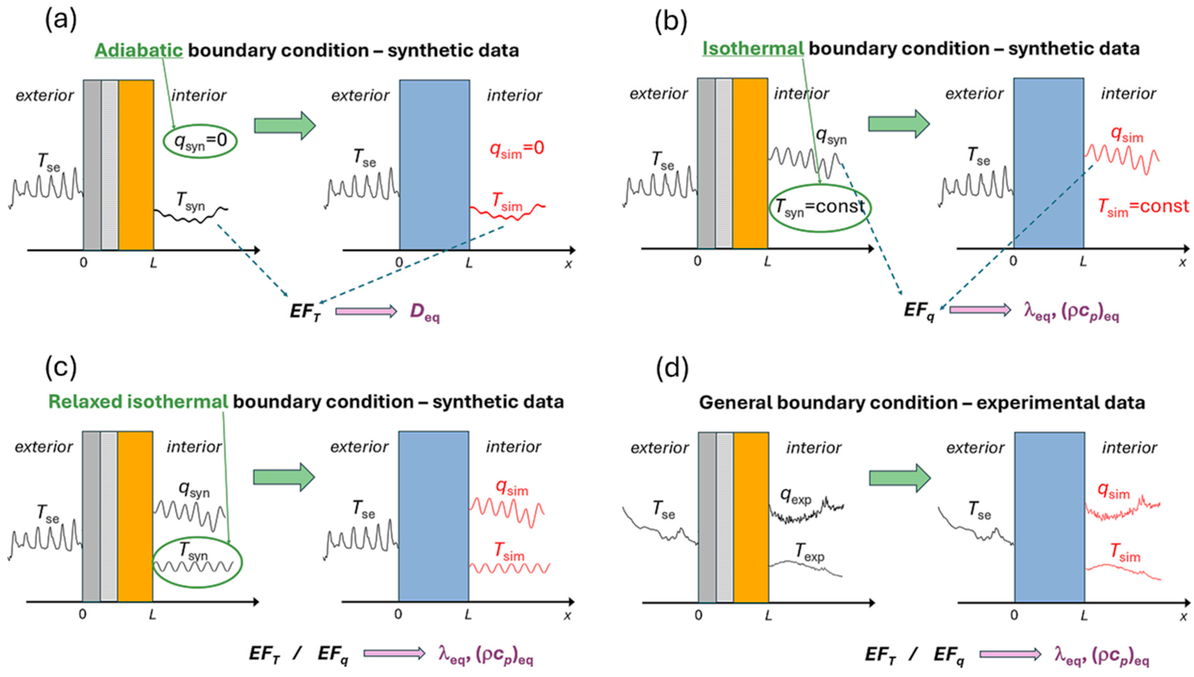
Depending on the inner boundary condition, the method identifies either a single equivalent parameter, i.e., thermal diffusivity (adiabatic case, Figure 1a) or two independent parameters, namely thermal conductivity and volumetric heat capacity, for isothermal (Figure 1b) and near-isothermal (Figure 1c) cases.

(v)

The robustness of the inverse identification is assessed by analyzing the sensitivity to deviations from ideal boundary conditions and by validating the approach against experimental data (Figure 1d).

The purpose of this section is therefore not to introduce additional methodological details, but to clarify the logical structure of the proposed approach, highlighting how boundary conditions determine both the number of identifiable equivalent parameters and the appropriate formulation of the inverse problem addressed in the subsequent sections.

2.1. Theoretical Framework

We address a homogeneous wall with constant thermophysical properties as a one-dimensional (1D) slab where heat propagates via conduction (see Figure 1 for the geometry of the problem), with no internal heat generation. The 1D Fourier equation then applies:

$$D{\displaystyle \frac{{\mathit{\partial }}^{2}T}{\mathit{\partial }{x}^2}}={\displaystyle \frac{\mathit{\partial }T}{\mathit{\partial }t}}$$

(1)

where D is thermal diffusivity. In general, the solution of the differential equation will be constituted by a steady-state part, $T_{\mathrm{s}\mathrm{s}}$, and a transient part, $T_{\mathrm{t}}$,

$$T\left(x,t\right)=T_{\mathrm{s}\mathrm{s}}\left(x,t\right)+T_{\mathrm{t}}\left(x,t\right)$$

(2)

with the latter depending on the imposed initial conditions and dying out after a sufficient time.

2.2. Duration of the Transient Thermal Response

In the determination of the equivalent wall parameters, it is necessary to compare quantities that are not affected by initial conditions. We therefore need to estimate the time required for the transient behavior to die out.

We can focus on two different boundary conditions at $x=L$: (a) the heat flux $q_L$ is zero (adiabatic boundary condition (BC)); (b) the face is kept at constant temperature $T_L$ (isothermal BC).

In case (a), within adiabatic BC, the quantity to consider at $x=L$ is temperature. Its transient part can be found to be [35]

$$T_{\mathrm{t} }\left(L,t\right)=\sum _{n=1}^{\infty }{\left(-1\right)}^{n-1}{B}_{n }{e}^{-D{\left[{\displaystyle \frac{\left(2n-1\right)\pi }{2L}}\right]}^{2}t}$$

(3)

with the coefficients $B_n$ given by

$$B_n={\displaystyle \frac{2}{L}}\underset{0}{\overset{L}{\int }}\left[T\left(x,0\right)-T_{\mathrm{s}\mathrm{s}}\left(x,0\right)\right]\sin \left[{\displaystyle \frac{\left(2n-1\right)\pi x}{2L}}\right]dx$$

(4)

The time constant that quantifies the dampening of the transient behavior can be estimated by assuming it is dominated by the first term of the summation above, which gives rise to

$${\tau }_{\mathrm{a}\mathrm{d}\mathrm{i}\mathrm{a}\mathrm{b}}={\displaystyle \frac{{4L}^2}{{\pi }^{2}D}}$$

(5)

At t = 3${\tau }_{\mathrm{a}\mathrm{d}\mathrm{i}\mathrm{a}\mathrm{b}}$ the temperature reaches 95% of the steady-state value.

In case (b), instead, we are interested in calculating the heat flux at $x=L$, which is given by

$$q\left(L,t\right)=-\lambda {\left({\displaystyle \frac{\mathit{\partial }T}{\mathit{\partial }x}}\right)}_{x=L}$$

(6)

where $\lambda$ is thermal conductivity. Its transient part can be written as

$$q_{t }\left(L,t\right)=-\lambda {\left({\displaystyle \frac{\mathit{\partial }{T}_t}{\mathit{\partial }x}}\right)}_{x=L}=-\lambda \sum _{n=1}^{\infty }{\displaystyle \frac{n\pi }{L}}{\left(-1\right)}^n{C}_{n }{e}^{-D{\left({\displaystyle \frac{n\pi }{L}}\right)}^{2 }t}$$

(7)

where the coefficients $C_{n }$ are given by

$$C_n={\displaystyle \frac{2}{L}}\underset{0}{\overset{L}{\int }}\left[T\left(x,0\right)-T_{\mathrm{s}\mathrm{s}}\left(x,0\right)\right]\sin \left({\displaystyle \frac{n\pi x}{L}}\right)dx$$

(8)

In this case, the time constant of the first mode is

$${\tau }_{\mathrm{i}\mathrm{s}\mathrm{o}\mathrm{t}\mathrm{h}}={\displaystyle \frac{L^2}{{\pi }^{2}D}}$$

(9)

For a given thermal diffusivity, the time constant required to dampen the transient behavior is therefore four times longer in adiabatic conditions than in isothermal conditions. In addition, when the model of the equivalent homogeneous wall is applied, it may be that different thermophysical parameters are determined to model the wall’s thermal behavior. It will be shown in the optimization section that, indeed, this is the case with the values obtained from the optimization. The transient duration estimation will then be further affected.

2.3. Number of Independent Equivalent Thermophysical Parameters

We show how many independent thermophysical parameters are needed to fully specify the dynamic thermal behavior of a homogeneous wall within the two limit BCs considered in the previous paragraph. To this end, we consider a thermal stimulus at the face $x=0$

$$T\left(0,t\right)=T_{\mathrm{m}}+A\cos \left(2\pi ft\right)$$

(10)

with a mean value $T_{\mathrm{m}}$ and a frequency $f=1/{\tau }_0$, where ${\tau }_0$, denotes the oscillation period, such as the daily temperature cycle.

In case (a) (adiabatic BC), the steady-state temperature $T_{\mathrm{s}\mathrm{s}}$ at $x=L$ is [35]

$$T_{\mathrm{s}\mathrm{s}}\left(L,t\right)=T_{\mathrm{m}}+A\left|G\right|\cos \left[2\pi ft-\mathrm{a}\mathrm{r}\mathrm{g}\left(G\right)\right]$$

(11)

where $G=1/\cosh \left(KL\right)$ and $K=(1+j)\sqrt{\pi f/D}$. It is apparent that only a single thermophysical parameter, the thermal diffusivity, D, affects the temperature at the inner face (at $x=L$). This statement is strictly correct only when the thermal input excitation is purely single-frequency, but it can also be considered appropriate when there is a dominant frequency, as in the case of daily temperature variations. In the following, we therefore use thermal diffusivity as the equivalent parameter to be determined for adiabatic BCs.

In case (b) (isothermal BC), the steady state heat flux $q_{\mathrm{s}\mathrm{s}}$ at $x=L$ (where the temperature is $T_L$) is

$$q_{\mathrm{s}\mathrm{s}}\left(L,t\right)={\displaystyle \frac{\lambda }{L}}\left(T_{\mathrm{m}}-T_L\right)+A|Y|\cos \left[2\pi ft-\mathrm{a}\mathrm{r}\mathrm{g}\left(Y\right)\right]$$

(12)

where $Y=\lambda K/\sinh \left(KL\right)$. In this case, the heat flux depends both on the thermal conductivity λ and on the thermal diffusivity D (by means of K), or, equivalently, on thermal conductivity and volumetric heat capacity $\rho c_p$.

3. Methodology

The methodology comprised an inverse identification of equivalent thermophysical parameters for a multilayer building wall by replacing it with a fictitious homogeneous 1D conduction model and calibrating its properties so that the inner-side dynamic response matches the reference wall under the same external forcing.

(1)

A high-fidelity multilayer reference response was generated:

(i)

Synthetic datasets were produced in COMSOL by simulating a 1D multilayer wall replicating the Perugia test wall stratigraphy and properties, driven at the outer boundary by measured hourly outdoor temperature over one year, and alternatively imposing an adiabatic inner boundary (inner heat flux set to zero) or an isothermal inner boundary (inner temperature fixed at 20 °C);

(ii)

Experimental datasets were taken from the University of Perugia test room, using measured outer/inner-surface temperatures and inner heat flux on the north wall.

(2)

The analysis explicitly removed initialization effects by estimating the decay of transients under each inner boundary condition and excluding a “warm-up” window from all objective-function evaluations (longer for adiabatic than for isothermal conditions).

(3)

An equivalent homogeneous wall model was simulated in COMSOL under the same boundary conditions, and its parameters were identified by maximizing a model efficiency factor (EF) computed on an inner-side response variable. For the adiabatic case (see Figure 1a), as shown in Section 2.2, theory indicates that the inner-surface temperature depends on a single independent parameter; accordingly, the equivalent thermal diffusivity was identified via a parameter sweep and selecting the diffusivity that maximized EF on inner-surface temperature over monthly calculations using two-month windows (with the initial warm-up excluded). For the isothermal case (Figure 1b), two independent parameters are required; therefore, thermal conductivity and volumetric heat capacity were jointly estimated (with specific heat capacity $c_p$ fixed) by coupling COMSOL time-dependent simulations with MATLAB Version 2024b’s constrained optimization (fmincon, interior-point), maximizing EF on the inner heat flux, using bounded parameters, multi-start initializations, and monthly evaluations after excluding the warm-up period.

(4)

Robustness to non-ideal inner conditions was assessed by generating additional synthetic datasets in which the inner temperature was prescribed as a daily sinusoid with varying amplitude (Figure 1c); the inverse identification was repeated using two alternative objective functions (temperature-based vs. heat-flux-based), demonstrating that heat-flux-based formulations remain well-posed in the near-isothermal limit.

(5)

Finally, the full framework was applied to experimental data (Figure 1d), considering months with markedly different inner boundary variability (e.g., non-isothermal vs. near-isothermal), comparing objective-function choices and reporting the resulting equivalent parameters and fit quality.

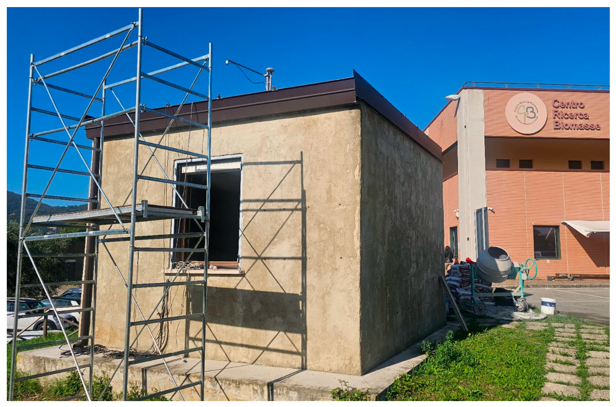
The experimental measurements were carried out in the test room constructed within the Engineering School of the University of Perugia. The facility, used as the case-study building, has dimensions of 3.78 m × 4.00 m × 2.85 m and is equipped with a comprehensive sensor network for monitoring both indoor and outdoor microclimatic conditions. In this study, heat flux and surface temperature data collected from sensors installed on the north-facing wall were employed. The stratigraphy and material properties of the wall are reported in

Table 1. Stratigraphy and thermophysical properties of the experimental test wall.

Stratigraphy	Thickness [m]	Thermal Conductivity [W/(mK)]	Specific Heat Capacity [J/(kgK)]	Mass Density [kg/m3]
Brickwork, outer leaf	0.12	0.41	800	1500
Plasterboard	0.01	0.16	950	700
High-density EPS insulation	0.09	0.04	1400	50
Brickwork, inner leaf	0.25	0.31	800	1500
Gypsum plastering	0.02	0.4	950	840

. The specific characteristics of the test room envelope components and a detailed description of the installed sensors are presented in [36]. Figure 2 illustrates the monitored test room.

3.1. Synthetic Data Generation

Synthetic data were generated in COMSOL Multiphysics^® 6.3 [37] by simulating the heat transfer in a one-dimensional multilayer wall replicating the real Perugia test wall in both stratigraphy and material properties. The outer boundary was driven by the measured hourly outdoor air temperature in Perugia for a full year (1 January 00:00 h–31 December 23:00 h) [38].

This was taken as the outer-surface temperature $T_{\mathrm{s}\mathrm{i}}\left(t\right)$. Two alternative inner boundary conditions were applied: (i) adiabatic dataset: inner heat flux fixed to zero ($q_L\left(t\right)=0$); (ii) isothermal dataset: inner temperature fixed at 20 °C ($T_{\mathrm{s}\mathrm{i}}\left(t\right)=20$°C).

Each simulation began with a steady-state computation using the first-hour outdoor temperature of 2013; the resulting temperature profile was then used as the initial condition for the time-dependent run. The time-dependent temperature is computed over the entire year (0 to 8759 h) with hourly outputs. The finite element mesh was set so fine that the results would not change upon decreasing mesh element size, ensuring mesh convergence. In the time-dependent solver, “intermediate” time-stepping was used: this instructs COMSOL to adapt time steps within user constraints (neither fully “free” nor “strict”), improving robustness on long-time runs while still maintaining limits on step size and order. The maximum time for the step size in the solver was set to 0.1 h (=6 min) to ensure a good enough resolution was obtained to detect the temporal change in the temperature field. 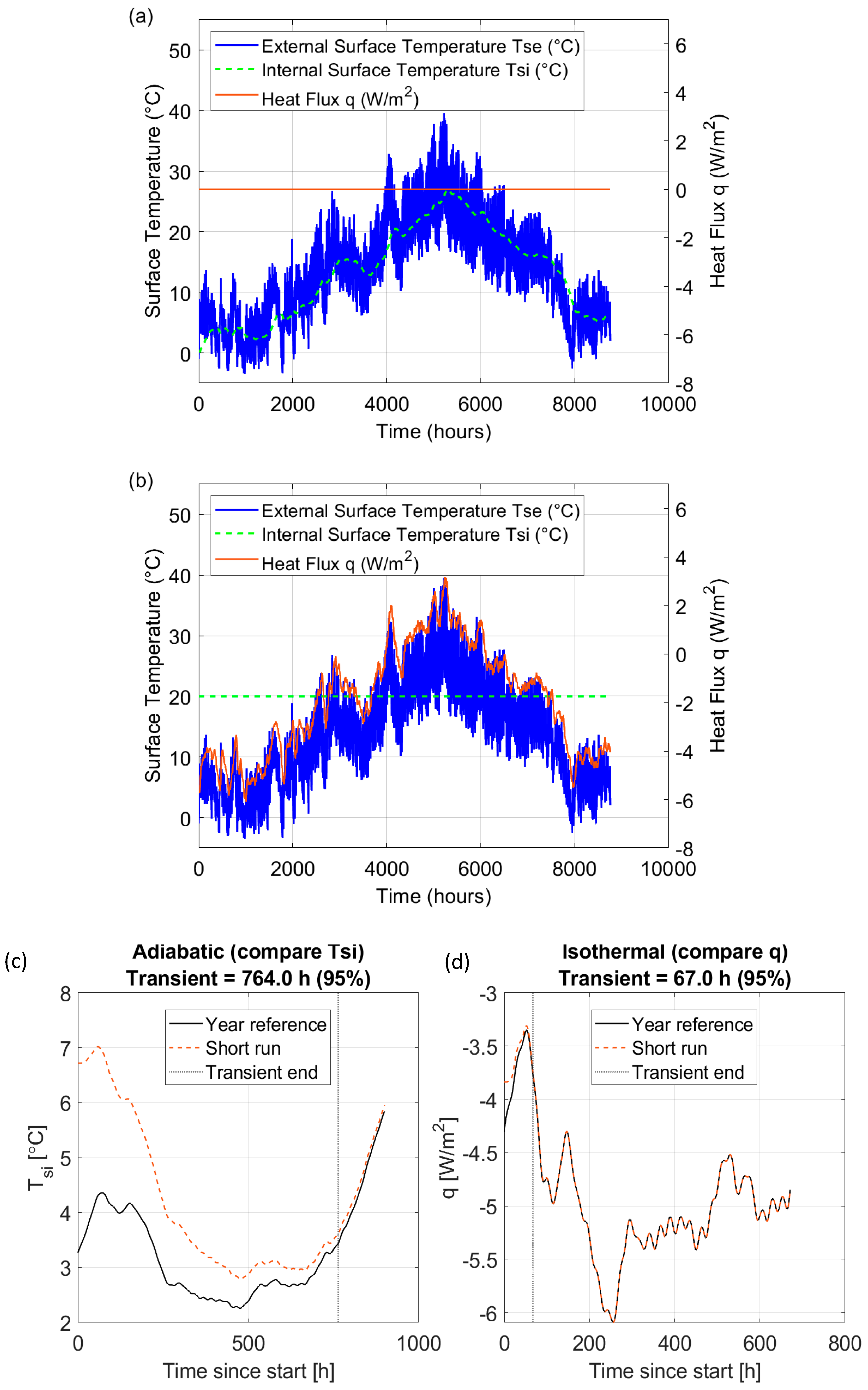Finally, the resulting inner-surface temperature $T_{\mathrm{s}\mathrm{i}}\left(t\right)$ and inner heat flux $q_L\left(t\right)$ were exported as the synthetic datasets; see Figure 3a,b.

To investigate the transient response, additional simulations were run, starting not on 1 January but on 1 February. The resulting inner wall temperature was compared to the full-year simulation and a transient (95% of steady state) of 764 h was found for the adiabatic case, while it was 67 h for the isothermal case; see Figure 3c,d. As shown in Section 2, due to the different nature of the inner boundary conditions, the transient response is markedly longer in the adiabatic case than in the isothermal one. In the isothermal configuration, the inner surface is clamped to 20 °C and effectively exchanges heat with an infinite-capacity reservoir, which rapidly damps any mismatch between the initial steady state and the subsequent dynamic regime. Conversely, in the adiabatic configuration, the inner surface is thermally insulated ($q_L=0$), so the energy entering the wall from the exterior can only be stored within the wall itself. The mean wall temperature therefore evolves more slowly, and the system retains a memory of the initial condition over a longer time horizon, leading to a longer warm-up period before a representative dynamic regime is established.

The values of the time constants 3τ, with τ calculated using Equations (5) and (9) and the estimated values of the thermal diffusivity, leading to 654 h (adiabatic) and 70 h (isothermal), in good qualitative agreement with the numerically estimated values. Therefore, the transient phase can be quite long under adiabatic boundary conditions. However, this is not the most common case in practical applications. Rather, an isothermal boundary condition is more frequently representative of real-world applications. In the latter case, the transient period is significantly shorter, typically not longer than a week.

3.2. Determination of Equivalent Thermophysical Parameters

The heat-transfer in a homogeneous equivalent wall model was simulated in COMSOL, similarly to the model generating the synthetic dataset used for comparison (see model details in the previous section on synthetic data generation). Because inverse optimization can be sensitive to solver-induced numerical noise, all COMSOL evaluations were performed with identical mesh and time-integration settings. The number of finite element mesh elements was 5, while the maximum time step size in the solver was 1 h; neither increasing the number of mesh elements nor decreasing the time step size improved the results of the inverse identification. In the solver, we used a relative tolerance of ${10}^{-2}$ and a global absolute tolerance of ${10}^{-3}\hspace{0.17em}\mathrm{K}$ for the dependent temperature variable. These settings were chosen to ensure a sufficiently smooth objective function for the reliable convergence of gradient-based optimizers when performing the inverse identification.

3.2.1. Adiabatic Dataset: Equivalent Thermal Diffusivity

For the adiabatic case, the thermal diffusivity D was targeted through a parameter sweep. For each D, the corresponding conductivity was computed as $\lambda =D\rho c_p$with fixed $\rho =250$ kg m⁻³ and $c_p=840$ J kg⁻¹K⁻¹. The specific values used for $\rho$ and $c_p$ do not affect the result when the temperature input is purely sinusoidal, as shown in Section 2.3. It was also verified that, even under realistic temperature stimuli, the dependence on their specific value is negligible in adiabatic conditions.

The match between the synthetic multilayer wall data and the homogeneous equivalent wall was quantified by the model Efficiency Factor ($EF$), evaluated on the inner-surface temperature

$${EF}_T=1-{\displaystyle \frac{{\sum }_i{\left(T_{\mathrm{s}\mathrm{i}\mathrm{m},i}-T_{\mathrm{s}\mathrm{y}\mathrm{n},i}\right)}^2}{{\sum }_i{\left(T_{\mathrm{s}\mathrm{y}\mathrm{n},i}-{\overline{T}}_{\mathrm{s}\mathrm{y}\mathrm{n}}\right)}^2}}$$

(13)

where $T_{\mathrm{s}\mathrm{i}\mathrm{m}}$ denotes the inner-surface temperature calculated with trial diffusivity values, $T_{\mathrm{s}\mathrm{y}\mathrm{n}}$, of the same quantity but obtained from the model of the actual multilayer structure, with ${\overline{T}}_{\mathrm{s}\mathrm{y}\mathrm{n}}$ as its mean value. The employment of the $EF$ index indicates that improved equivalent models can be identified, going beyond the ASHRAE standard, as shown in [31].

Because of the long transient period associated with the insulated inner surface, the first 764 h of each run (approximately one month) was excluded from the ${EF}_T$ computation. Consequently, the simulations were performed over two-month windows shifted by one month each (starting January → February → … → November) to ensure that each evaluation included an established steady-state dynamic regime while covering the entire annual sequence. The optimal diffusivity $D_{\mathrm{e}\mathrm{q}}$was defined by the maximum of ${EF}_T\left(D\right)$.

3.2.2. Isothermal Dataset: Inverse Identification of $\lambda$ and $\rho$

For the isothermal dataset ($T_{si}$ = 20 °C), the thermophysical parameters to be estimated are the thermal conductivity $\lambda$ and the volumetric heat capacity $\rho c_p$. Regarding the latter, only the product of density $\rho$ and specific heat capacity $c_p$ influences the dynamic thermal response. However, COMSOL requires $\rho$ and $c_p$ to be specified separately. For this reason, we fixed one of the two parameters ($c_p$) to an arbitrary value, i.e., $c_p=$ 840 J kg⁻¹K⁻¹, and performed the optimization on the other ($\rho$). In practice, the optimization takes place in a two-dimensional parameter space and identifies $\lambda$ and $\rho$, which is fully equivalent to determining $\lambda$ and the volumetric heat capacity $\rho c_p$. MATLAB’s fmincon (interior-point) algorithm was used for the optimization, whereas COMSOL performed the time-dependent computation and returned EF on the heat flux on the inner wall surface. In this case, the EF is therefore

$${EF}_q=1-{\displaystyle \frac{{\sum }_i{\left(q_{\mathrm{s}\mathrm{i}\mathrm{m},i}-q_{\mathrm{s}\mathrm{y}\mathrm{n},i}\right)}^2}{{\sum }_i{\left(q_{\mathrm{s}\mathrm{y}\mathrm{n},i}-{\overline{q}}_{\mathrm{s}\mathrm{y}\mathrm{n}}\right)}^2}}$$

(14)

with $q_{\mathrm{s}\mathrm{i}\mathrm{m}}$ being the inner heat flux calculated with trial $\lambda$ and $\rho$ values, $q_{\mathrm{s}\mathrm{y}\mathrm{n}}$the inner heat flux calculated from the model of the actual multilayer structure, and ${\overline{q}}_{\mathrm{s}\mathrm{y}\mathrm{n}}$ its mean value. We used fmincon with gradients estimated by finite differences. Since the objective is obtained from a COMSOL simulation followed by post-processing (i.e., an implicit, solver-defined function), analytical derivatives would require implementing parameter sensitivities/adjoint methods; given that there are only two decision variables, the additional function evaluations for finite differences are acceptable.

Parameter bounds were $0.05\le \lambda \le 0.50$W m⁻¹K⁻¹ and $50\le \rho \le 1200$ kg m⁻³; a multi-start grid of initial guesses ensured robustness. To be conservative, a warm-up period of 150 h was excluded in each monthly ${EF}_q$ evaluation to eliminate the effect of the transient build up.

4. Results and Discussion

4.1. Adiabatic Case

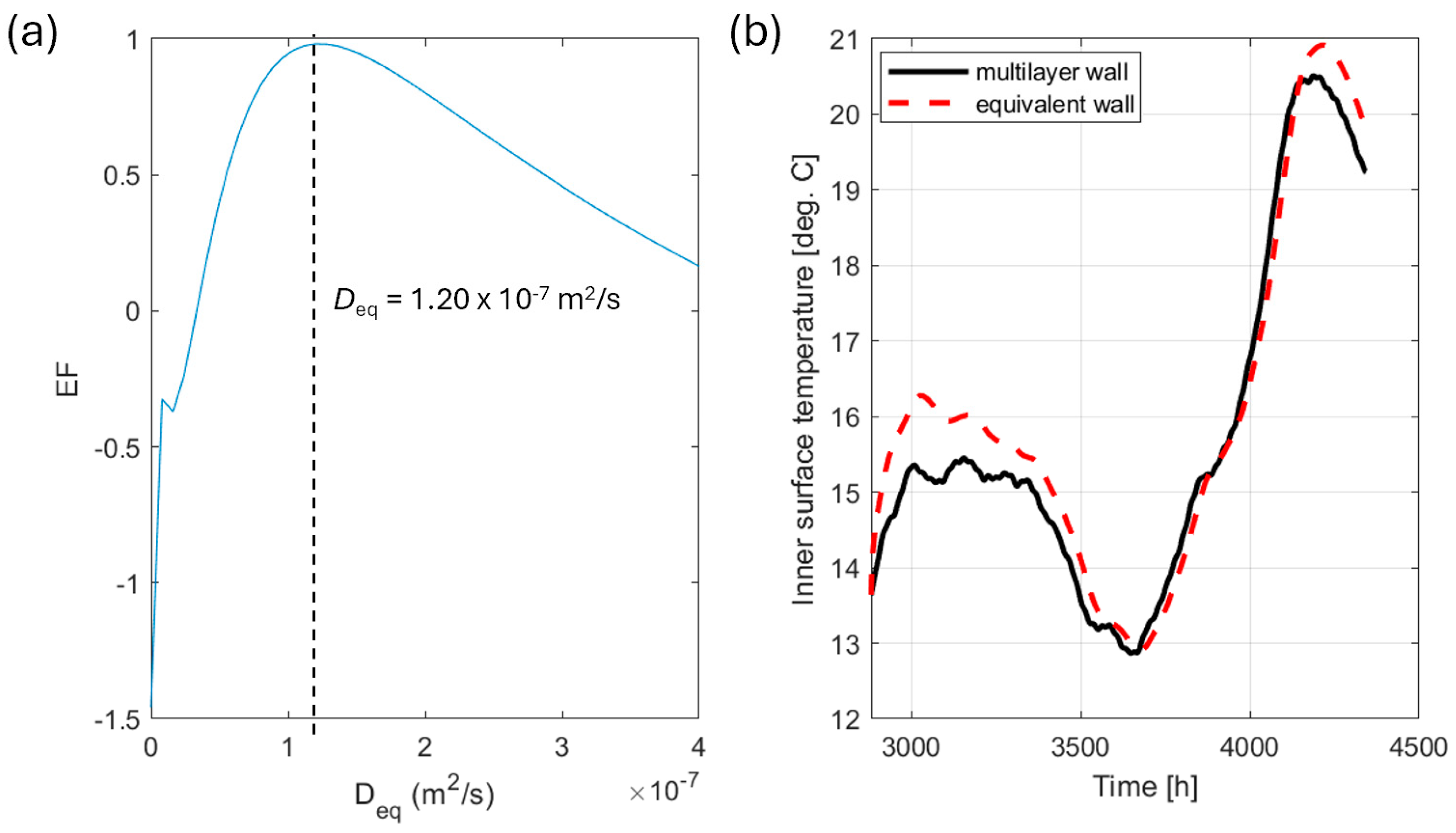
Figure 4 illustrates the identification of the equivalent thermophysical parameters for the adiabatic configuration—specifically, the results of the May–June dataset are shown. The inner-surface temperature of the multilayer reference wall (black solid line) is compared with that of the equivalent homogeneous wall (red dashed line), obtained by varying the thermal diffusivity $D_{\mathrm{e}\mathrm{q}}$ until the ${EF}_T$ is maximized. The ${EF}_T$curve in Figure 4a shows a clear, single optimum, confirming a well-posed identification problem. The optimal equivalent diffusivity is $D_{\mathrm{e}\mathrm{q}}=1.20\times {10}^{-7}$ m²/s, yielding an efficiency $E{F}_T=0.98$. Across the entire annual analysis, the optimal value of $D_{\mathrm{e}\mathrm{q}}$ remains within $1.1-1.4\times {10}^{-7}$ m²/s, while $E{F}_T$ values typically exceed 0.9. The mean value is $D_{\mathrm{e}\mathrm{q}}\approx 1.24\pm 0.07\times {10}^{-7}$ m²/s. The agreement between the simulated and reference temperatures shown in Figure 4b is very good: the equivalent wall captures both the amplitude and phase of the inner-surface temperature response, with only minor overprediction during the largest peaks. The small phase lag differences are physically consistent with the simplification from a multilayer to a single-layer model.

Overall, the adiabatic configuration confirms that a single equivalent diffusivity can reliably reproduce the dynamic temperature behavior of the multilayer wall under insulated boundary conditions. The long transient observed before the steady periodic regime, requiring a 764 h-long warm-up exclusion, is intrinsic to the adiabatic condition, where energy entering the wall can only be stored internally, delaying equilibrium.

4.2. Isothermal Case

As a reference to the identification of the thermophysical parameters using the optimization approach, the Efficiency Factor ${EF}_q$ was first simulated as a function of the thermal conductivity and mass density in expected ranges; see Figure 5, where Panel (a) shows only the ${EF}_q$ values between 0 and 1, while Panel (b) shows the ${EF}_q$ values in the full range from −19 to 1.

Figure 5 indicates that ${EF}_q$ is more sensitive to variations in thermal conductivity than to variations in mass density.

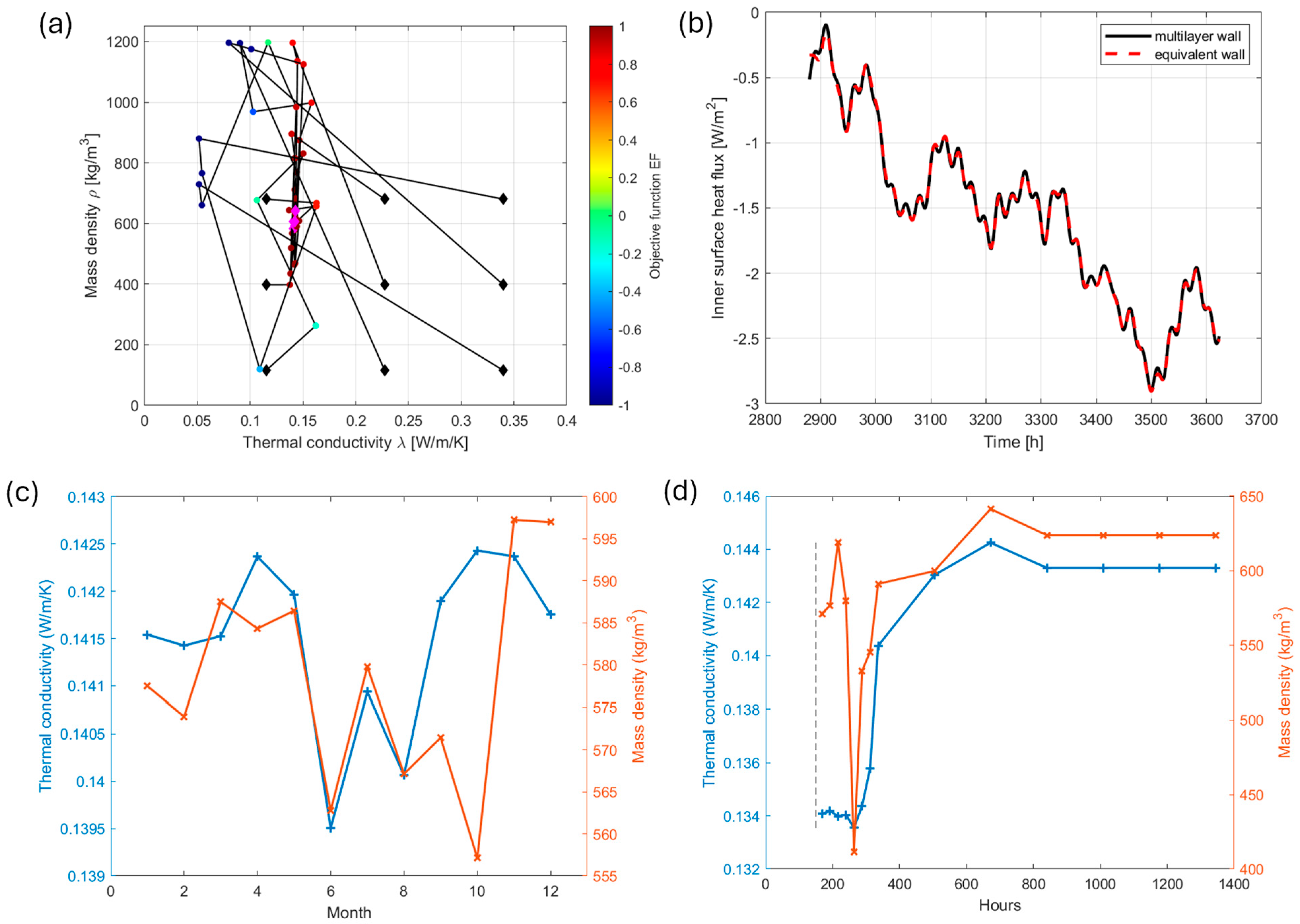
Figure 6 summarizes the identification of the equivalent thermophysical parameters for the isothermal configuration, using the January dataset (with approximately the first week excluded) as a representative example. Panel (a) shows the evolution of the optimization process in the λ–ρ parameter space, where the model efficiency factor ${EF}_q$ on the inner heat flux was used as the objective function. The algorithm converges consistently toward a narrow high-efficiency region, confirming the presence of a unique optimum. The best-fit parameters were ${\lambda }_{\mathrm{e}\mathrm{q}}$ = 0.142 W m⁻¹ K⁻¹ and ${\rho }_{\mathrm{e}\mathrm{q}}$ = 577 kg m⁻³, corresponding to ${EF}_q$ = 0.999. Notice that the data in Table 1 provides an equivalent thermal conductivity value of ${\lambda }_{\mathrm{e}\mathrm{q},\mathrm{t}\mathrm{h}\mathrm{e}\mathrm{o}}=L/{\sum }_i(L_i/{\lambda }_i)= 0.142$ W m⁻¹ K⁻¹, in excellent agreement with the optimized value. Panel (b) of Figure 6 compares the simulated and reference inner-surface heat fluxes for the multilayer and equivalent walls. The agreement is nearly perfect: both the amplitude and phase of the heat-flux signal are accurately reproduced. Similar results were obtained for all months, with ${EF}_q$ values consistently above 0.995 and only marginal variations in the optimal parameters (${\lambda }_{\mathrm{e}\mathrm{q}}=$ 0.140–0.142 W m⁻¹ K⁻¹, ${\rho }_{\mathrm{e}\mathrm{q}}=$ 560–600 kg m⁻³); see Figure 6c. The stability of the equivalent parameters across the full year demonstrates the robustness of the numerical inverse method and the COMSOL–MATLAB coupling. The mean equivalent thermal diffusivity is $D_{\mathrm{e}\mathrm{q}}={\displaystyle \frac{{\lambda }_{\mathrm{e}\mathrm{q}}}{{\rho }_{\mathrm{e}\mathrm{q}}{c}_p}}\approx 2.91\pm 0.06\times {10}^{-7}$ m²/s. This value is slightly more than twice the value in the adiabatic configuration, reflecting the more direct conductive heat exchange imposed by the fixed-temperature boundary condition. This reduced value of the equivalent diffusivity—together with the factor of 4, which scales the isothermal time constant (see Equation (9)) compared with the adiabatic one (Equation (5))—explains the significantly shorter time needed to extinguish the transient in isothermal BC.

To assess the influence of dataset length on the stability of the inverse identification, the isothermal analysis was repeated while progressively extending the duration of the synthetic dataset. Figure 6d shows the resulting estimates of ${\lambda }_{\mathrm{e}\mathrm{q}}$ and ${\rho }_{\mathrm{e}\mathrm{q}}$ as a function of the total number of hours included in the optimization. A vertical dashed line marks the 150 h warm-up period, after which ${EF}_q$ is evaluated. Consequently, all reported points lie to the right of this threshold: shorter datasets would not contain any usable data once the warm-up window is removed. The results reveal clear convergence behavior. For very short datasets (just above the warm-up threshold), the identified parameters exhibit noticeable variability due to the limited amount of dynamic information that is available. As the dataset length increases beyond approximately 400–600 h, both ${\lambda }_{\mathrm{e}\mathrm{q}}$ and ${\rho }_{\mathrm{e}\mathrm{q}}$ stabilize rapidly and remain effectively constant for all longer windows. At 114 h after the transient cut (264 h total), ${\rho }_{\mathrm{e}\mathrm{q}}$deviates 34.0% from its converged value, while at 186 h after the transient cut, it has fallen to just 5.26%. Similarly, at 114 h and 186 h after the transient cut, ${\lambda }_{\mathrm{e}\mathrm{q}}$ deviates 6.84% and 2.09% from its converged value, respectively. Consequently, if the transient cut is reduced to 80 h (see Figure 3d), an inverse identification in stable isothermal-like conditions with 5% or less accuracy can be obtained in 266 h = 11 days.

4.3. Sensitivity of the Inverse Identification to Deviations from Isothermal Boundary Conditions

To evaluate the robustness of the inverse identification beyond the idealized isothermal configuration, additional synthetic datasets were generated by relaxing the constant inner-surface temperature condition. The inner boundary was prescribed as a periodic temperature

$$T_{\mathrm{s}\mathrm{i}}\left(t\right)=T_{\mathrm{m}}+T_{\mathrm{a}\mathrm{m}\mathrm{p}\mathrm{l}}\mathrm{c}\mathrm{o}\mathrm{s}\left({\displaystyle \frac{2\pi t}{{\tau }_0}}\right)$$

(15)

where $T_{\mathrm{m}}=20$ °C, ${\tau }_0=86400$ s and $T_{\mathrm{a}\mathrm{m}\mathrm{p}\mathrm{l}}$denotes the amplitude of the imposed daily temperature oscillation. This formulation introduces a controlled deviation from isothermal conditions while preserving a realistic daily timescale. The oscillation amplitude was varied over a wide range $T_{\mathrm{a}\mathrm{m}\mathrm{p}\mathrm{l}}= \left\{0.01,0.10,1,2, \dots ,15\right\} °\mathrm{C}$, spanning from nearly isothermal ($T_{\mathrm{a}\mathrm{m}\mathrm{p}\mathrm{l}}=0.01 °\mathrm{C}$) to strongly time-dependent ($T_{\mathrm{a}\mathrm{m}\mathrm{p}\mathrm{l}}=15 °\mathrm{C}$) inner boundary conditions.

For each dataset, the inverse identification described in Section 3.2.2 was applied to estimate the equivalent thermal conductivity $\lambda$ and mass density $\rho$, with the specific heat capacity $c_p$ fixed. Two objective functions were considered: (i) ${EF}_T$, comparing inner-surface temperature while prescribing heat flux, and (ii) ${EF}_q$, comparing inner-surface heat flux while prescribing temperature. A warm-up period of 150 h was excluded from the EF evaluation to remove initial transients.

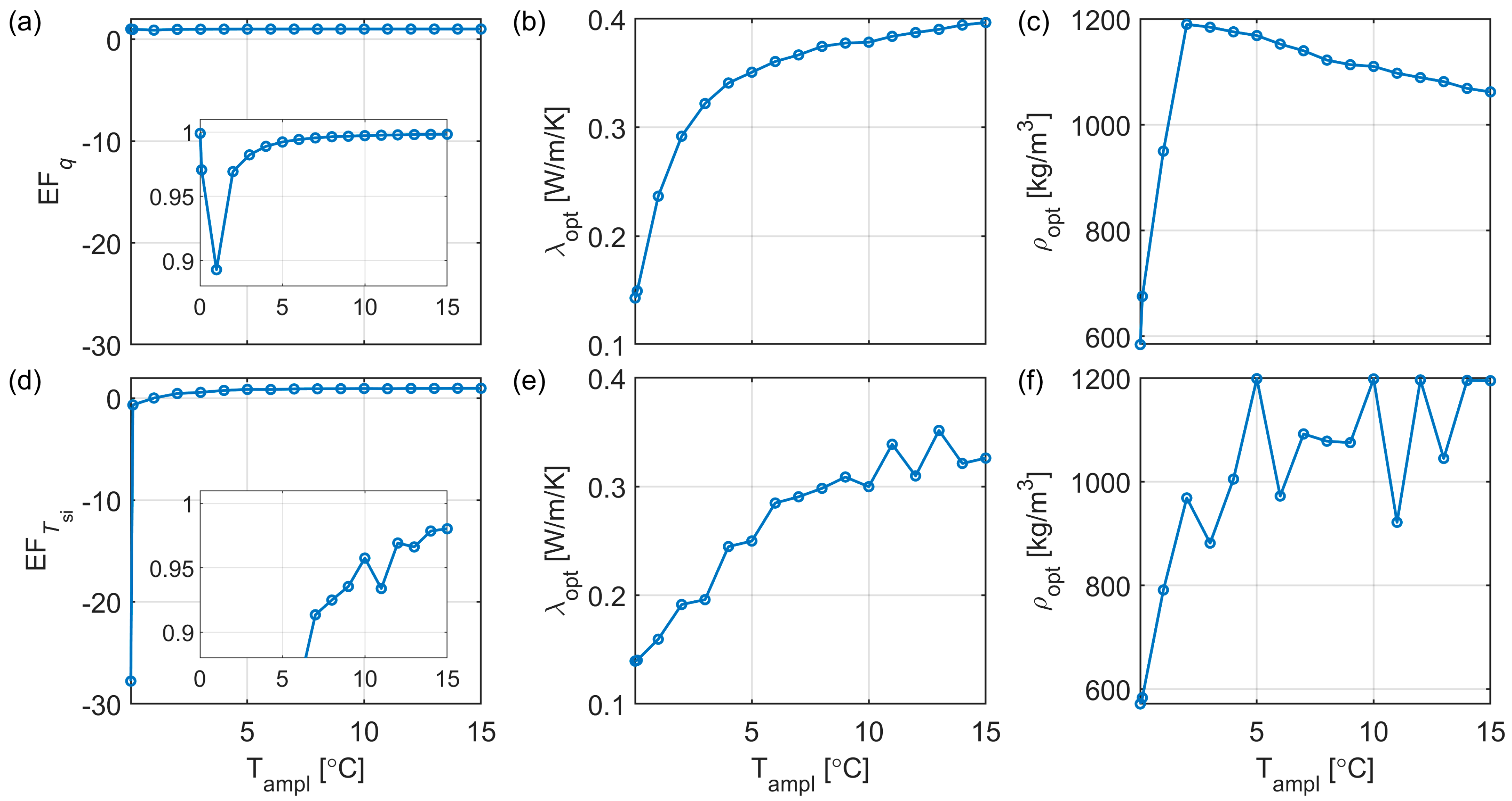
The results show that the inverse identification based on ${EF}_T$ (Figure 7d–f) becomes increasingly ill-conditioned as the oscillation amplitude $T_{\mathrm{a}\mathrm{m}\mathrm{p}\mathrm{l}}$ decreases. For small values of $T_{\mathrm{a}\mathrm{m}\mathrm{p}\mathrm{l}}$, the inner boundary condition approaches the strictly isothermal limit, and the temporal variance of $T_{\mathrm{s}\mathrm{i}}$becomes very small. In this regime, the denominator of the EF definition ${\sum }_i{\left(T_{\mathrm{s}\mathrm{y}\mathrm{n},i}-{\overline{T}}_{\mathrm{s}\mathrm{y}\mathrm{n}}\right)}^2$, tends toward zero, causing ${EF}_T$ to diverge. This behavior is identical to that observed in the strictly isothermal case, where ${EF}_T$ is mathematically undefined due to the absence of temperature variability at the inner surface. Consequently, this results in poor optimization performance for small $T_{\mathrm{a}\mathrm{m}\mathrm{p}\mathrm{l}}$ as ${EF}_T$ is much more sensitive.

For larger oscillation amplitudes, where the inner-surface temperature exhibits appreciable temporal variation, ${EF}_T$ yields a more stable optimization. However, even in this regime, the sensitivity of the temperature signal to the internal wall properties remains limited, leading to a relatively flat objective landscape and non-unique optimal solutions.

In contrast, the inverse identification based on $E{F}_q$ (Figure 7a–c) remains well-posed over the entire range of oscillation amplitudes investigated. When the inner-surface temperature is prescribed according to the periodic boundary condition and the heat flux is used as the comparison variable, the optimization consistently converges toward stable $\lambda$ and $\rho$ values. Importantly, the performance of $E{F}_q$ does not deteriorate in the near-isothermal limit. Even when $T_{\mathrm{a}\mathrm{m}\mathrm{p}\mathrm{l}}$ is small, the heat flux response retains sufficient variability and sensitivity to the wall’s thermal inertia and conductivity, ensuring a well-defined objective function and robust parameter recovery.

The analysis highlights a fundamental distinction between temperature-based and heat-flux-based objective functions. While ${EF}_T$ becomes ill-defined in the strictly isothermal and near-isothermal limits due to normalization effects, ${EF}_q$ remains stable and informative across both constant and periodically varying inner boundary conditions.

4.4. Experimental Test Results

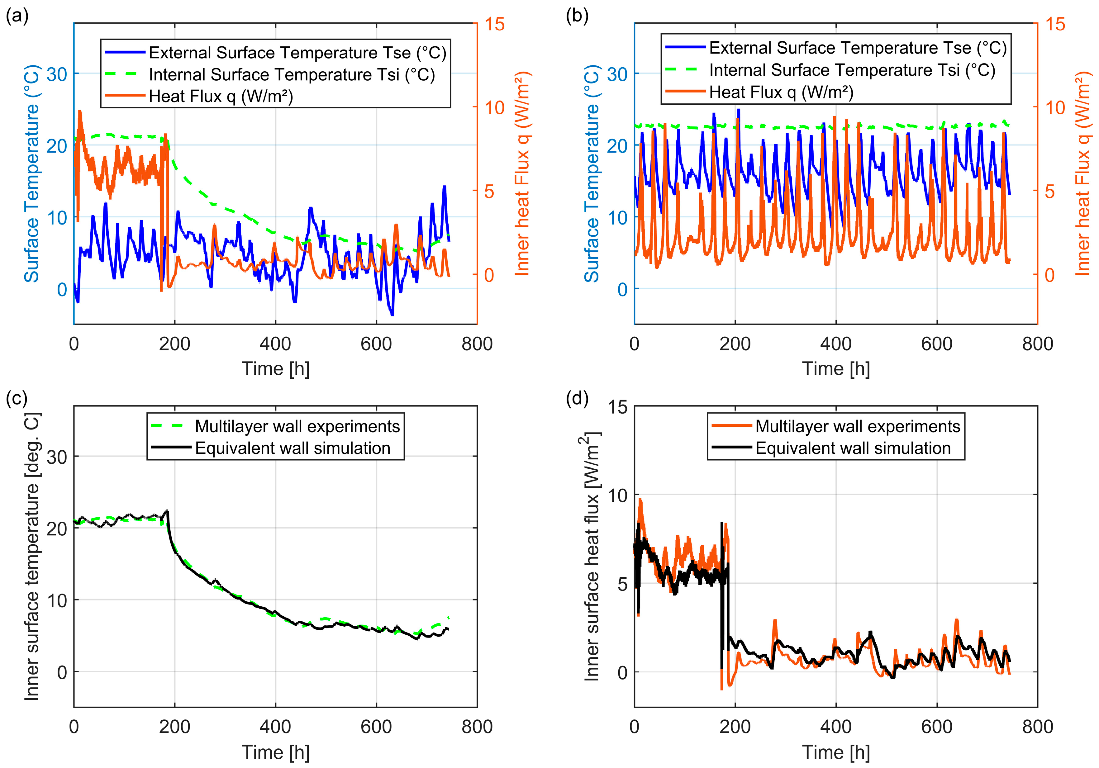
The optimization framework was evaluated using experimental data recorded in the test room built at the University of Perugia. Two representative months were selected: January and October, chosen to reflect markedly different inner-surface boundary conditions. January is characterized by a strongly time-varying inner-surface temperature $T_{\mathrm{s}\mathrm{i}}$, whereas October corresponds to a heating period with $T_{\mathrm{s}\mathrm{i}}$ close to isothermal.

Figure 8a shows the measured external surface temperature $T_{\mathrm{s}\mathrm{e}}$, inner-surface temperature $T_{\mathrm{s}\mathrm{i}}$, and inner-surface heat flux $q$for January. In this case, the pronounced temporal variations in $T_{\mathrm{s}\mathrm{i}}$ indicate a clearly non-isothermal boundary condition. The corresponding data for October are shown in Figure 8b, where $T_{\mathrm{s}\mathrm{i}}$ remains tightly controlled over time due to active heating.

For each month, the inverse problem was solved using two objective functions: ${EF}_T$, with heat flux $q_{\mathrm{e}\mathrm{x}\mathrm{p}}$ imposed as a boundary condition, and $E{F}_q$, with inner-surface temperature $T_{\mathrm{e}\mathrm{x}\mathrm{p}}$as prescribed. The $EF$ definitions used with the experimental data were therefore

$${EF}_T=1-{\displaystyle \frac{{\sum }_i{\left(T_{\mathrm{s}\mathrm{i}\mathrm{m},i}-T_{\mathrm{e}\mathrm{x}\mathrm{p},i}\right)}^2}{{\sum }_i{\left(T_{\mathrm{e}\mathrm{x}\mathrm{p},i}-{\overline{T}}_{\mathrm{e}\mathrm{x}\mathrm{p}}\right)}^2}}$$

(16)

$${EF}_q=1-{\displaystyle \frac{{\sum }_i{\left(q_{\mathrm{s}\mathrm{i}\mathrm{m},i}-q_{\mathrm{e}\mathrm{x}\mathrm{p},i}\right)}^2}{{\sum }_i{\left(q_{\mathrm{e}\mathrm{x}\mathrm{p},i}-{\overline{q}}_{\mathrm{e}\mathrm{x}\mathrm{p}}\right)}^2}}$$

(17)

The resulting optimized parameters and objective function values are summarized in

Table 2. Estimated parameters and objective function values from the experimental data.

Mode	Month	${\mathit{\lambda }}_{\mathbf{o}\mathbf{p}\mathbf{t}}$ [W/(m K)]	${\left(\mathit{\rho }{\mathit{c}}_{\mathit{p}}\right)}_{\mathbf{o}\mathbf{p}\mathbf{t}}$ [J/(K m3)]	EF [−]
${EF}_T$	January	0.183	6.12 × 105	0.98
${EF}_T$	October	0.176	10.0 × 105	−5.76
${EF}_q$	January	0.169	4.25 × 105	0.78
${EF}_q$	October	0.193	1.72 × 105	0.63

.

For January, both formulations yield physically plausible estimates of the effective thermal conductivity and mass density, with $EF$ values close to unity. This behavior is consistent with the synthetic results for non-isothermal and periodically forced inner boundary conditions, confirming that sufficient temperature dynamics ensure a well-posed inverse problem.

For October, the performance diverges significantly. When using ${EF}_T$, the optimization becomes ill-conditioned, leading to non-physical parameter estimates and extreme $E{F}_T$ values. This behavior is a direct consequence of the near-isothermal inner boundary condition: as shown in previous sections, the denominator of ${EF}_T$ approaches zero under isothermal conditions, causing the objective function to diverge. This does not indicate a fundamental incompatibility of the inverse problem, but rather a limitation of ${EF}_T$ in this regime.

In contrast, $E{F}_q$ remains stable and robust for both months, yielding consistent and physically meaningful parameters even under near-isothermal conditions. These experimental results confirm the conclusions drawn from the synthetic studies and demonstrate that $E{F}_q$ is the preferred objective function when the inner-surface temperature is controlled or weakly varying, as is common in real building operations.

In both the temperature-based and heat flux-based estimations of the thermal conductivity, the parameter to which the inner quantities exhibit the highest sensitivity is close to the theoretical value, ${\lambda }_{\mathrm{e}\mathrm{q},\mathrm{t}\mathrm{h}\mathrm{e}\mathrm{o}}= 0.142$ W m⁻¹ K⁻¹. The slightly larger estimated values are consistent with the aging of the materials.

5. Conclusions

The identification of equivalent thermophysical parameters of a multilayer wall by means of a homogeneous one-dimensional conduction model was addressed in this study. The primary objective was to investigate the extent to which the simplified model is capable of capturing the dynamic thermal behavior of a real multilayer wall, while accounting for the effect of different inner boundary conditions, including adiabatic, isothermal, and more general cases. The number of independent parameters to be estimated and the choice of the objective function used for inverse identification were justified.

Analytical considerations and numerical simulations demonstrated that the duration of the transient thermal response strongly depends on the imposed inner boundary condition. Adiabatic conditions lead to significantly longer transients than isothermal conditions, a result that was quantitatively established by synthetic simulations and shown to be consistent with theoretical predictions. This finding highlights the necessity of excluding sufficiently long warm-up periods when comparing the simulated and reference data, especially in insulated configurations.

For adiabatic boundary conditions, the dynamic behavior of the wall can be reliably characterized by a single equivalent parameter, namely the thermal diffusivity. The identification problem was shown to be well-posed, yielding a clear and stable optimum with high efficiency factors throughout the year. The equivalent homogeneous wall accurately reproduces the inner-surface temperature trend, despite the simplification of the model.

In contrast, under isothermal boundary conditions, two independent parameters are required to describe the wall dynamics. The coupled inverse identification of thermal conductivity and volumetric heat capacity proved to be robust and stable when based on the inner-surface heat flux as the comparison quantity. The optimized parameters exhibited minimal seasonal variability and converged rapidly as the dataset length increased beyond a few hundred hours. An inverse identification in stable isothermal-like conditions with 5% or less accuracy was obtained in approximately 11 days. A more detailed treatment of the frequency dependence of the equivalent thermophysical properties will be dealt with in future work.

It is also important to emphasize that the duration of the transient phase, the warm-up period associated with the imposed inner boundary condition, differs significantly between the two idealized setups. In the case study considered, the transient lasted approximately one month under adiabatic boundary conditions, whereas with the isothermal configuration, which is more commonly representative of real-world applications, the transient period did not exceed one week.

A key result of this work concerns the sensitivity of the inverse identification to deviations from ideal isothermal conditions. Temperature-based objective functions become ill-conditioned at the strictly isothermal or near-isothermal limit, due to the vanishing variance of the inner-surface temperature signal. In contrast, heat-flux-based objective functions remain well-defined and informative over the entire range of investigated boundary conditions, including both constant and periodically varying inner-surface temperatures.

The application to experimental data from a test wall confirms the conclusions drawn from the synthetic analyses. While both temperature-based and heat-flux-based formulations perform satisfactorily under strongly non-isothermal conditions, only the heat-flux-based approach provides stable and physically meaningful results when the inner-surface temperature is tightly controlled, as commonly occurs in real buildings.

Overall, the results demonstrate that the identifiability of equivalent thermophysical parameters is not only governed by the wall structure, but also critically depends on the boundary conditions and on the formulation of the objective function. From a practical perspective, heat-flux-based inverse methods emerge as the most robust choice for the characterization of building envelope components under realistic operating conditions.

In addition, this type of modeling is devised as a simple means for evaluating the building’s performance, in which the envelope transmission heat load, a direct function of internal heat flux, represents a key quantity. This is a further point that supports a heat-flux-based inverse method for the identification of equivalent parameters. The proposed method is designed to provide end users with practically useful information that can be directly employed as an input in building energy simulation software. It requires only the use of surface sensors and relies on an automatic data post-processing procedure that estimates the equivalent thermophysical properties of the investigated component under the applied boundary conditions.

In the usual in situ applications, the external boundary condition results from combined convection, radiation, and shortwave absorption, which may in turn partially affect the values of the equivalent thermophysical parameters. In our setup, the measured outer-surface temperature was imposed to eliminate uncertainties in the external heat-flux model and ensure a controlled excitation for the inverse problem. For applications involving different external conditions (e.g., distinct convection, radiation, or solar loads), the same identification procedure can be repeated with boundary conditions representative of the target scenario. The issue of transferability between distinct realistic scenarios will be addressed in future work.