


Abstract
Research related to the use of hydrogen is crucial because it can be a significant factor in reducing exhaust emissions into the environment. This work represents the second stage of research related to the analysis of exhaust gases from a miniature GTM 400 MOD turbojet engine. Based on the parameters obtained in the experiment, a numerical study of the flow downstream of the exhaust nozzle was performed in ANSYS software (version R1, 2025). The main goal of the calculations was to obtain the temperature distribution and compare the values at checkpoints where actual measurements were taken. The study was conducted in two stages. In the first stage, the engine operated conventionally, burning kerosene. In the second stage, co-combustion of kerosene and hydrogen occurred in the engine. The numerical analysis enabled the visualization of the flow phenomenon for these stages within the considered rotational speeds. The analysis examined flow in domains where the gap was included and excluded. This gap was created by the different diameters of the container opening and the engine nozzle outlet. The study showed that ignoring the gap allows for temperatures closer to the experimental values. Results deemed satisfactory were less likely to be found in vortex areas, but more likely in areas closer to the container walls and the engine exhaust stream itself. The results of the conducted tests showed that the Root Mean Square Error RMSE was within the range of 9.5–22.8% relative to the average temperature values obtained from experimental measurements. The highest turbulence intensity occurred for hydrogen co-combustion at a higher rotational speed, reaching 284% for Variant 2 and 300% for Variant 1. The largest standard deviation for both fuel types at a distance of 0.083 m from the container wall was 68.5 K for variant 2 and 76 K for variant 1. At a distance of 0.166 m from the container wall, the deviation was 76 K for variant 2 and 83.8 K for variant 1.
Keywords:
co-combustion; hydrogen; numerical analysis; turbojet engine; CFD; combustion diagnostics; RANS 1. Introduction
Engine research is currently one of the most important fields of study in the development of aviation technology. This involves continuous engine improvement, as well as its optimization in terms of fuel composition changes and the possible future use of alternative fuels, such as hydrogen. Such research can result in newly observed phenomena, which may lead to new design solutions. The existence of these phenomena can be proven primarily experimentally, but also using modern mathematical tools that solve the scientific problem through approximation, depending on the model used.
The integration of pressure gain combustion into aeroengine systems has gained increasing attention as a promising pathway to significantly enhance thermal efficiency. In this context, the study by Varatharajulu and Stathopoulos [1] presents a thermodynamic and exergy-based comparison of turbojet and turbofan engines equipped with a Rotating Detonation Combustor (RDC). Although their findings confirm potential performance benefits, the analysis relies on simplified cycle modeling and does not consider the complex flow interactions downstream of the nozzle, leaving unresolved questions regarding exhaust dynamics and structural loading.
In pursuit of alternatives to complex vectoring systems for Short Take-Off and Landing STOL applications, Zhang et al. [2] demonstrated the potential of a bypass dual throat nozzle with a bending transition duct. While their results highlight thrust vectoring feasibility, the absence of structural and unsteady flow assessments limits understanding of how such concepts would affect nozzle outlet turbulence and long-term operability. Similarly, Meng et al. [3] investigated serpentine-configured multi-stream supersonic nozzles, identifying stealth advantages at the expense of thrust. However, the lack of experimental validation or optimization studies leaves a gap in understanding how such flow distortions translate to thermomechanical impacts on nozzle walls.
Ensuring stable combustion under unconventional conditions was addressed by He et al. [4], who examined water injection in Turbine-Based Combined Cycle TBCC engines. Their combined experimental and numerical study shows improved stability, but the research remains restricted to specific regimes and does not explore how altered exhaust properties propagate through downstream nozzle sections. In parallel, Aygun et al. [5] compare metaheuristic optimization strategies for small turbojet cycles, revealing trade-offs in thrust and fuel consumption. However, these optimizations assume idealized operation, neglecting secondary effects such as structural loads or turbulent mixing in exhaust jets.
Efforts to integrate hydrogen into aviation fuels have also exposed critical challenges. Niszczota and Gieras [6] demonstrated that hydrogen inlet injection can reduce CO2 emissions but increases NOx formation, while long-term nozzle durability remains unaddressed. Ayaz et al. [7] provide comparative insights into kerosene, diesel, and JP-4, identifying environmental trade-offs but without assessing how fuel chemistry alters exhaust flow and structural constraints. At the combustor level, Kang et al. [8] proposed a combined injection scheme that improves detonation efficiency but also increases pulsating exhaust pressures, which could amplify nozzle thermal and mechanical stresses, yet this aspect is not explicitly analyzed.
The off-design behavior of micro gas turbines has been studied by Wu et al. [9], who achieved improved accuracy with corrected maps. While effective for performance prediction, their method does not provide detailed flow-field resolution at the nozzle exit. Zhang et al. [10] further contributed with a multi-modal combustor design, but their system-level simulations lack downstream validation, limiting their applicability for nozzle thermomechanical studies. Xu et al. [11] introduced a rotor-motion-coupled CFD framework, reducing prediction errors under crosswind conditions, but its high computational cost constrains systematic nozzle load assessments under fuel variation.
On the broader energy landscape, Boretti [12] emphasizes hydrogen’s potential in aviation while acknowledging persistent barriers, particularly in combustion stability and NOx mitigation. Yet, as highlighted, much of the literature remains conceptual, with limited integration of fuel chemistry effects on exhaust nozzle flow, temperature fields, and material stresses.
Addressing these gaps more directly, Brodzik et al. [13] conducted a detailed thermomechanical analysis of the GTM 400 MOD turbojet nozzle operating on kerosene and kerosene–hydrogen co-combustion, supported by coupled CFD/FEM modeling. Their results confirmed that hydrogen addition did not significantly increase nozzle wall temperature or deformation, with peak temperatures below 1100 K and stresses remaining within the material yield limit. These values are consistent with the present findings for comparable engine speeds, indicating that the temperature rise induced by hydrogen enrichment is moderate and does not exceed thermal safety margins. However, Brodzik et al. [13] focused primarily on structural aspects, without analyzing the spatial evolution of the exhaust flow field beyond the nozzle exit.
Bogoi et al. [14] offered complementary insight into flow and acoustic behavior in micro turbojet exhausts using chevron and ejector nozzles. Their Schlieren imaging revealed strong local gradients and vortex formation near the nozzle exit, corresponding to flow structures similar to those observed in the present numerical results. Nevertheless, their work addressed noise attenuation rather than thermal or pressure field coupling, leaving the thermofluid interaction effects unexplored.
Related experimental investigations by Catana and Badea [15] demonstrated that variations in exhaust nozzle geometry significantly affect the operating line and thrust characteristics of gas turbine engines, indirectly confirming the strong sensitivity of downstream flow structures to geometric modifications. However, their analysis focused on global performance parameters and did not resolve local temperature or turbulence distributions in the exhaust region.
Similarly, Villarreal-Valderrama et al. [16] investigated thrust augmentation through a variable exhaust nozzle using active disturbance rejection control, showing that controlled nozzle geometry variations can strongly influence engine thrust and stability. While their results highlighted the dynamic coupling between nozzle configuration and engine performance, detailed thermofluid field analysis downstream of the nozzle was beyond the scope of their study.
In contrast, the present work explicitly quantifies temperature, pressure, and turbulence fields in a confined exhaust environment, thereby complementing these studies by providing spatially resolved thermofluid insight into the effects of exhaust geometry and operating conditions.
Ciupek et al. [17] previously conducted an experimental investigation of the GTM400 MOD turbojet engine operating under kerosene–hydrogen co-combustion, focusing on the measurement of exhaust gas temperature, emission composition (CO2, CO, NOx), and thrust variation at two rotational speeds (31,630 rpm and 47,110 rpm). Their results demonstrated a temperature increase proportional to the hydrogen share in the fuel mixture, reaching up to 760 K, and confirmed corresponding reductions in CO2 and CO emissions alongside an increase in NOx due to thermal effects. The present study therefore represents the second stage of this research, extending the earlier experimental findings through numerical modeling of the flow downstream of the exhaust nozzle, where pressure distribution, turbulence intensity, and aerodynamic structures were analyzed for the same engine configurations and operating parameters established in [17].
Overall, compared to these studies, the present numerical analysis advances understanding by correlating temperature and pressure field development behind the nozzle with fuel composition effects, bridging the gap between thermomechanical modeling [13], acoustic investigations [14], and emission-oriented experiments [17].
Taken together, these works underline both the potential and the limitations of current research on alternative fuels and nozzle configurations. Despite recent advances in thermodynamic modeling, cycle optimization, and partial hydrogen integration in aviation propulsion, a significant research gap remains in the field of high-fidelity characterization of flow structures and thermomechanical interactions downstream of miniature turbojet nozzles operating under kerosene–hydrogen co-combustion. Filling this gap is essential for understanding how alternative fuels modify the exhaust-jet behavior of temperature, and turbulence generation factors that directly influence emission control, structural loads, and the durability of next-generation propulsion systems.
A review of the literature indicates that very limited experimental or numerical information exists on the detailed representation of exhaust-jet development behind turbojet nozzles, particularly for engines operating at small scales. Where such studies exist, they typically address conventional kerosene combustion, while comprehensive analyses for kerosene–hydrogen mixtures are absent. This lack of data complicates validation of numerical models and hinders the development of generalized predictive tools for hydrogen-enriched fuels.
In this context, the primary objective of the present study is to clearly characterize the exhaust-flow behavior downstream of a miniature turbojet nozzle operating under kerosene and kerosene–hydrogen co-combustion. The scientific significance of this work lies in its integration of dedicated experimental measurements with validated numerical modeling, enabling a detailed analysis of temperature distribution, total pressure field evolution, and turbulence intensity in regions where no such data have previously been available. By providing this combined framework, the study contributes to establishing a foundation for future development of generalized models describing exhaust-jet structure under alternative-fuel operation.
This work constitutes the second part of a broader research effort devoted to the characterization of the exhaust-gas plume of a miniature turbojet engine and its diagnostic interpretation. While previous studies in the field of turbojet engine combustion diagnostics have primarily focused on radiative heat transfer modeling in combustion environments [18,19] or on advanced non-contact diagnostic techniques applied to engine components and dynamic responses [20]. The present study provides a novel contribution by delivering a quantitative, experimentally validated numerical description of the flow and temperature field downstream of the exhaust nozzle.
The originality of this work lies in bridging the gap between combustion-oriented diagnostics and downstream exhaust analysis by demonstrating that key thermofluid characteristics of the exhaust plume can be accurately reproduced without explicit combustion modeling, using experimentally derived boundary conditions. In this way, the study complements existing combustion diagnostics approaches by extending their applicability to confined exhaust regions, offering new insights that support the validation and refinement of future theoretical and computational models of miniature turbojet engines.
2. Materials and Methods
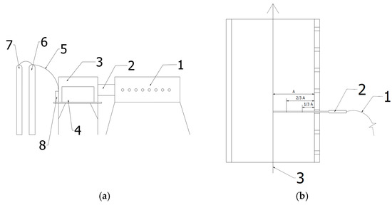
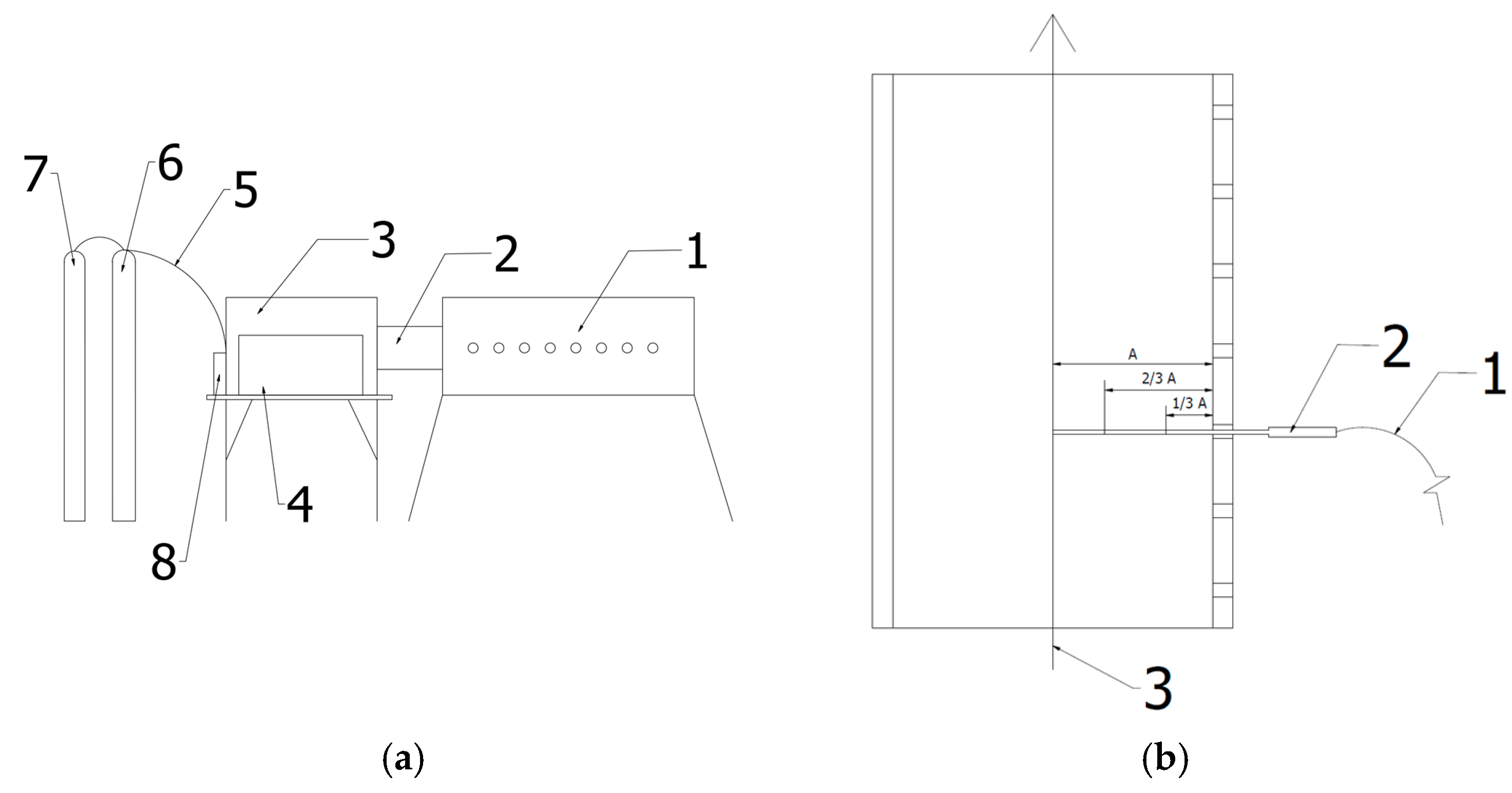
The numerical analysis was performed using ANSYS Fluent software (version R1, 2025). It was intended to illustrate the exhaust flow in a specially designed container attached to a turbojet engine (Figure 1a). The test stand was equipped with connection points for the temperature measurements (1), an exhaust gas outlet from the engine (2), a GTM400 turbojet engine stand (3), the GTM400 turbojet engine (4), a fuel connection (5), a kerosene tank (6), a hydrogen tank (7) and a fuel mixing and dosing system (8). The probing temperatures stand (Figure 1b) was equipped with thermoelectric temperature sensors type K (1–2), measuring the temperature transversely to the direction of exhaust gas flow (3).
Figure 1.
The test stand: (a) engine stand with container; (b) scheme of probing temperatures in the exhaust gas (A = ±250 mm) [17].
In reality, during the test, the engine was placed in a container whose diameter on the engine side was 0.13 m. In the case of the engine, the nozzle end diameter was 0.12 m. Due to this difference, there was a gap where air could freely flow between the container interior and the test stand environment. Therefore, two calculation variants were adopted in the analysis:
- Variant 1—the existence of a gap related to the difference in the mentioned diameters was taken into account, Figure 2.
- Variant 2—a simplification was applied, consisting of eliminating the gap, then the diameter of the nozzle end cross-section was equal to the diameter of the container.
Figure 2.
Location of checkpoints in the container [17].
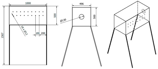
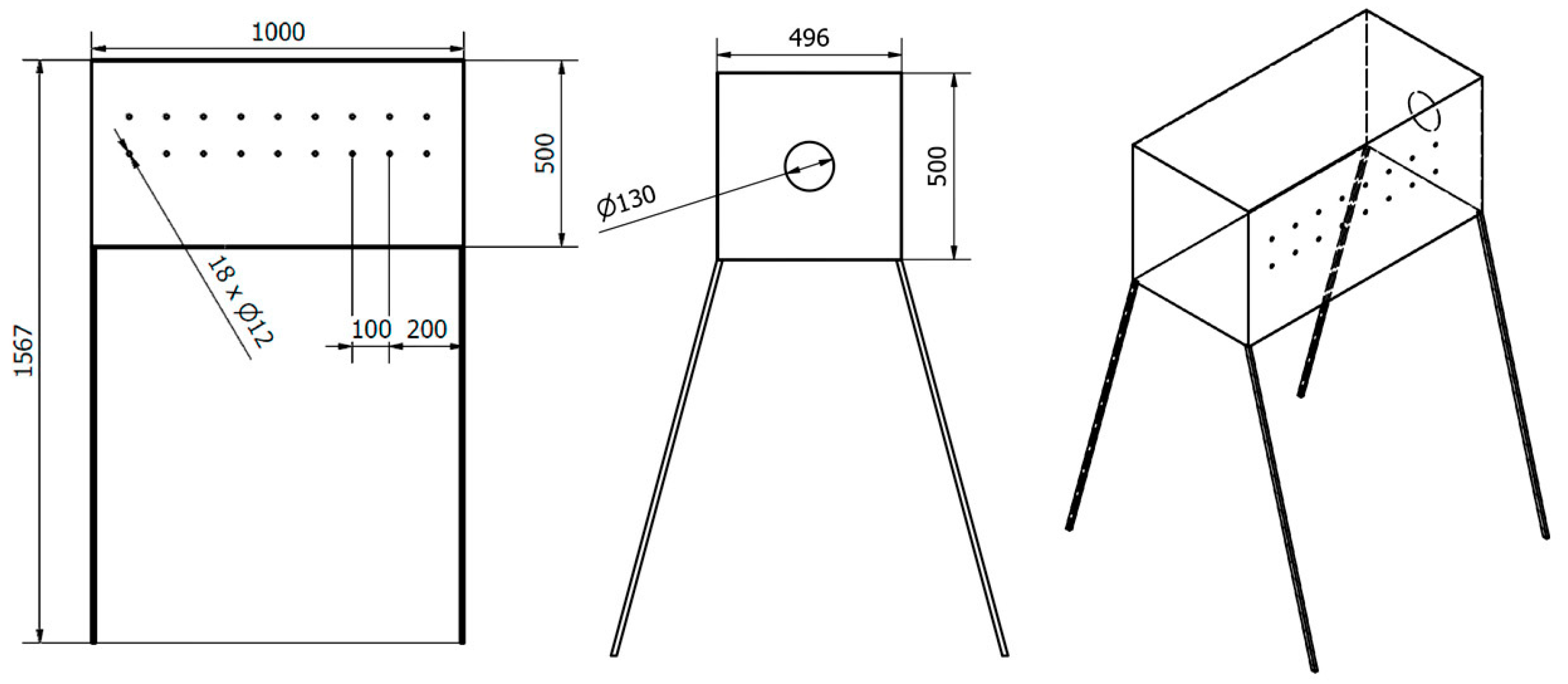
The container’s dimensions for length, width, and height (excluding the stand) were 1 m, 0.496 m, and 0.5 m, respectively. Its outlet was unobstructed. The dimensions of the air-filled space behind the container were 3 m, 1.5 m, and 1.5 m.
2.1. GTM400 MOD Turbojet Engine
The calculations concern the GTM400 MOD turbojet engine manufactured by JetPol (Poznań, Poland). This is a miniature single-flow engine, modernized to enable combustion of a kerosene–hydrogen mixture in the combustion chamber. The engine specifications are shown in Table 1. Hydrogen supply was provided by a hydrogen system with hydrogen cylinders manufactured by Linde Gaz Polska (Poznań, Poland). The engine uses Jet A-1 kerosene and 99.955% pure hydrogen. The numerical analysis was based on experimental measurements, in which the flow conditions were determined as follows: For the co-combustion of kerosene and hydrogen, the kerosene flow was reduced to 85% each time. At this time, kerosene mass flow rate was 228 mL/min for the lower speed and 306 mL/min for the higher speed. Simultaneously, the hydrogen flow was started, which was 149 L/min for the lower speed and 393 L/min for the higher speed. Hydrogen was injected into the return duct near the inlet to the vaporizers. The engine control panel was responsible for kerosene control. A 2000 SLPM flow regulator from Alicat Scientific (Tucson, AZ, USA) was installed at the gas system outlet. The pressure regulators were designed to reduce the system pressure to 8 bar. The flow regulator was calibrated for this pressure and maintained the highest accuracy there. For pressure and temperature, the accuracy was 0.5% and 0.75 °C, respectively. The measured flux range for this device is 2000 SLPM (standard liters per minute). In this way, after feeding the kerosene and hydrogen mixture, the same rotational speed was achieved as when burning kerosene alone. More detailed data related to the gas system and the engine are described in the literature [17,21]. Initial conclusions regarding engine operation with kerosene–hydrogen co-combustion were also formulated there.
Table 1.
The engine specifications.
2.2. Experimental Studies Behind the Nozzle
The numerical simulation was performed based on experimental data presented in Table 2. The measured volumetric flow rate at the nozzle takes into account both the mass of the supplied air and the mass of the fuel burned in the combustion chamber. Tests were performed for two engine speeds: 31,630 rpm and 47,110 rpm. At the lower speed, the kerosene-fueled engine produced 14.7% less thrust than when fueled with kerosene and hydrogen. At the higher speed, the difference was similar, 8.4% less thrust. During engine operation, temperature was measured behind the nozzle using thermoelectric sensors. To measure the flue gas temperature, 18 K-type (NiCr–Ni) thermocouples were used, with a measurement range of 73 K to 1274 K. Based on the calibration of the entire measurement system, the temperature measurement uncertainty in the range of 373 K to 773 K did not exceed ±1.2 K. Temperature measurements were taken in three zones (distances) from the engine nozzle. In each zone, the measurement was taken along the engine’s axis of symmetry and closer to the container housing wall. A more precise arrangement of the measurement points, hereinafter referred to as checkpoints, is presented in Figure 2. More detailed information about the experiment is provided in the literature [17].
Table 2.
Experimental data.
To confirm the reliability of temperature measurements, all thermocouples were calibrated before the experimental campaign using a certified dry-block temperature calibrator with an accuracy of ±0.5 K and cross-checked against a platinum resistance reference thermometer. Calibration was carried out at three temperature points: 373 K, 573 K, and 773 K, covering the full range expected during testing. Each measurement series was repeated three times under the same conditions to assess repeatability, with variations between repetitions remaining within ±1.2 K. Calibration and verification were performed both prior to and after the engine tests to ensure sensor stability and to minimize the influence of possible signal drift.
2.3. Input Data for Numerical Analysis
The engine operated for an extended period at the same speed, fueled with kerosene and hydrogen at constant, set values. Simultaneously, temperature measurements were taken at various checkpoints at the same time. Therefore, the steady flow condition was used for the calculations. Flow modeling requires solving the basic equations of fluid mechanics. The first is the continuity equation:
where is the fluid density, , is time, , and are velocity vectors in the Cartesian coordinate system, .
The second is the momentum equation:
where is the stress tensor is the external force, .
The third is the energy equation:
where is the specific heat, J/(kgK), is the temperature, K, a s the thermal conductivity coefficient, W/mK.
Additionally, the real combustion process requires solving the diffusion equation that takes into account the combustion reaction. This formula, in simplified form, is as follows:
where is the diffusion coefficient, m2/s, is the concentration of the reacting substance, kg/m3, is the term describing the combustion reaction, kg/(m3s).
For calculations of real flows, i.e., those that take viscosity into account, RANS (Reynolds Averaged Navier–Stokes) models are used, among others. In such an analysis, the time-averaged Navier–Stokes equations are solved. This simplification shortens the computational time. These models simulate the behavior of disturbed, vortex flow in various ways, often depending on their complexity. The SST k–ω model was used for flow analysis. Using a blending function, it combines the k–ω model near the wall and the k-ε model further from the wall, where free flow occurs. The standard k–ω model and the transformed k-ε model are multiplied by the mixing function and added [13,22]. In this case, the turbulent viscosity accounts for the transport of turbulent shear stress. Combining both models reduces sensitivity to turbulence in the free inlet flow and allows for more versatile calculation options [23,24]. Appropriate calculations in both layers (models) are possible due to the presence of a damped term of the cross-diffusion derivative in the ω equation. The k–ω Shear Stress Transport (SST) model contains two equations [25,26]:
- (a)
- the specific turbulent kinetic energy for [m2s−2]
- (b)
- the specific turbulent dissipation rate (also specific turbulent frequency) for ω [s−1]
The first blending function is given by the equation
is the cross-diffusion term [kgm−1s−2]
is turbulent length scale [m]
The function is equal to 0 outside the boundary layer and equal to 1 inside the boundary layer. Its values depend, among other things, on i ω.
is the kinematic eddy viscosity [m2s−1]
where is constant, is the strain norm, and is the second mixing function
In places with large shear gradients, the overestimation of the value limits the expression in the denominator .
is the effective rate of production [kgm−1s−3]
and prevents the formation of turbulence in stagnation areas, where
According to the above, the specific turbulent kinetic energy and the specific turbulent dissipation rate ω are coupled to each other via the modified eddy viscosity , the production and , the dissipation and the cross-diffusion term. The k-ϵ model constants used in the calculations were , TKE , TDR , Energy , Wall , where is the Prandtl number.
The energy model was used in the calculations, and thermal radiation was included in the flow. The conservation of the radiative energy along a ray path of direction can be written as
where —radiative intensity at a point with coordinates , and direction determined by the unit vector , —extinction coefficient, —coefficient of absorption, —coefficient of scattering, —scattering phase function, —refractive index, —solid angle.
The radiation equation was solved by approximation, using discrete ordinates. A pressure-based solver was used, and the air density was given a constant. During the analysis, the domain was described by boundary conditions. At the inlet, the experimentally obtained mass flow and temperature were assumed, which, in simplified terms, was equal to the value measured at the closest distance from the nozzle, within the container. Atmospheric pressure of 101,325 Pa and temperature of 300 K were assumed for the slot inlet. The same values were determined at the container outlet. The container walls were assumed to be made of steel, the density of which was 8030 kg/m3. Air density was 1.225 kg/m3. Other material properties of the container and air are presented in Table 3. The assumed material properties are assumed and adopted as for 316 steel. The adiabatic condition was used for the outer walls of the container. The numerical analysis undertaken did not take into account the fuel combustion process in a turbojet engine. Therefore, the flow stream studied was a mixture of air, kerosene, and hydrogen. Therefore, the paper does not present any information regarding the composition of the exhaust gases. The analysis was therefore a simplification aimed at reproducing the temperature field downstream of the engine nozzle as faithfully as possible.
Table 3.
The container material and air properties.
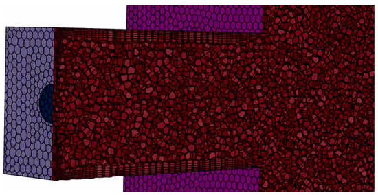
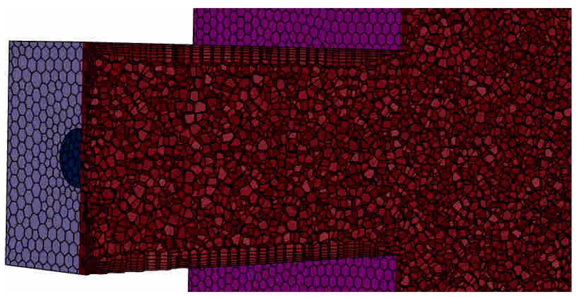
An unstructured mesh filled with polyhedral elements was used in the calculations. The number of mesh elements for variant 1 was 815,117, while for variant 2 it was 804,054. These grids were adopted after the validation stage described in the next section. An example mesh is presented in Figure 3. An example parameter for assessing mesh quality, i.e., orthogonal quality, for variant 1 was 0.693, while for variant 2 it was 0.615. These were the minimum values for both parameters. The average y+ value along the container walls was 4.62. The number of layers installed was 5 and the growth rate was 1.15.
Figure 3.
The domain Mesh—Variant 4, close-up of the container area.
3. Domain Validation
Before conducting the main analysis, a model validation was performed based on five sample meshes. The tests included simulations for a test engine operating at 47,110 rpm with a kerosene–hydrogen co-combustion. The domain was constructed according to the assumptions of Variant 2. In this case, its dimensions were as follows:
- (a)
- D-1: container dimensions, i.e., 1 m, 0.496 m, and 0.500 m, variant 2;
- (b)
- D-2: container dimensions and the space behind its outlet: 3 m, 1.5 m, 1.5 m, variant 2;
- (c)
- D-3: container dimensions and the space behind its outlet: 4 m, 1.5 m, 1.5 m, variant 2;
- (d)
- D-4: container dimensions and the space behind its outlet: 6 m, 1.5 m, 1.5 m, basic mesh, variant 2;
- (e)
- D-5: container dimensions and the space behind its outlet: 6 m, 1.5 m, 1.5 m, dense mesh, variant 2;
- (f)
- D-6: container dimensions and the space behind its outlet: 6 m, 1.5 m, 1.5 m, basic mesh, variant 1;
- (g)
- D-7: container dimensions, the space behind its outlet: 6 m, 1.5 m, 1.5 m, and the space around the slot 0.5 m long with external limits 1.5 m wide and 1.5 m high, variant 1.
In each case, the dimensions are given in the following order: length, width, and height. Each subsequent case considered involved a more complex computational domain. For variant 2, the domain dimensions were increasingly increased, and in case D-5, additional mesh refinement was performed. The selected parameters for each mesh are presented in Table 4. The minimum orthogonality was not less than 0.51 and the maximum skewness did not exceed 0.489. These values were considered acceptable taking into account the degree of simplification of the domain and boundary conditions. These are also parameters generally considered acceptable or good. An additional analysis involved comparing two models, namely the Realizable k-ε and the SST k–ω. In this case, a domain with 1,031,894 finite volumes was used. The minimum orthogonality was 0.57 and the minimum skewness was 0. The domain consisted of a portion of the container and the space behind the container, each measuring 3 m, 1.5 m, and 1.5 m. The Realizable k-ε model differs from the k-ε model in two respects. First, it provides an alternative formulation for turbulent viscosity. Second, it has a modified transport equation for epsilon dissipation. For these reasons, this model can better simulate regions of highly sheared flow.
Table 4.
Selected parameters for mesh evaluation.
The validation of the computational domain was performed based on the determination of the mean absolute error according to the equation
where is the number of numbers in the set, is the temperature measured during the experiment at the checkpoint [K], and is the temperature calculated during simulation at the checkpoint [K].
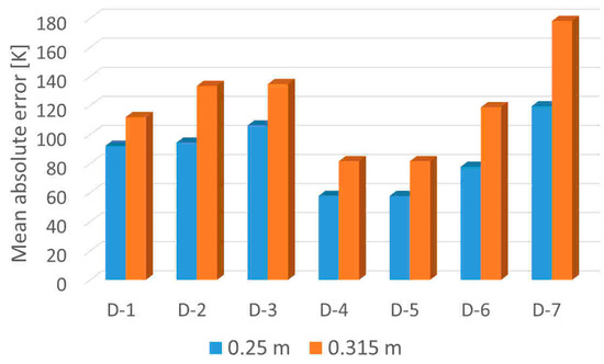
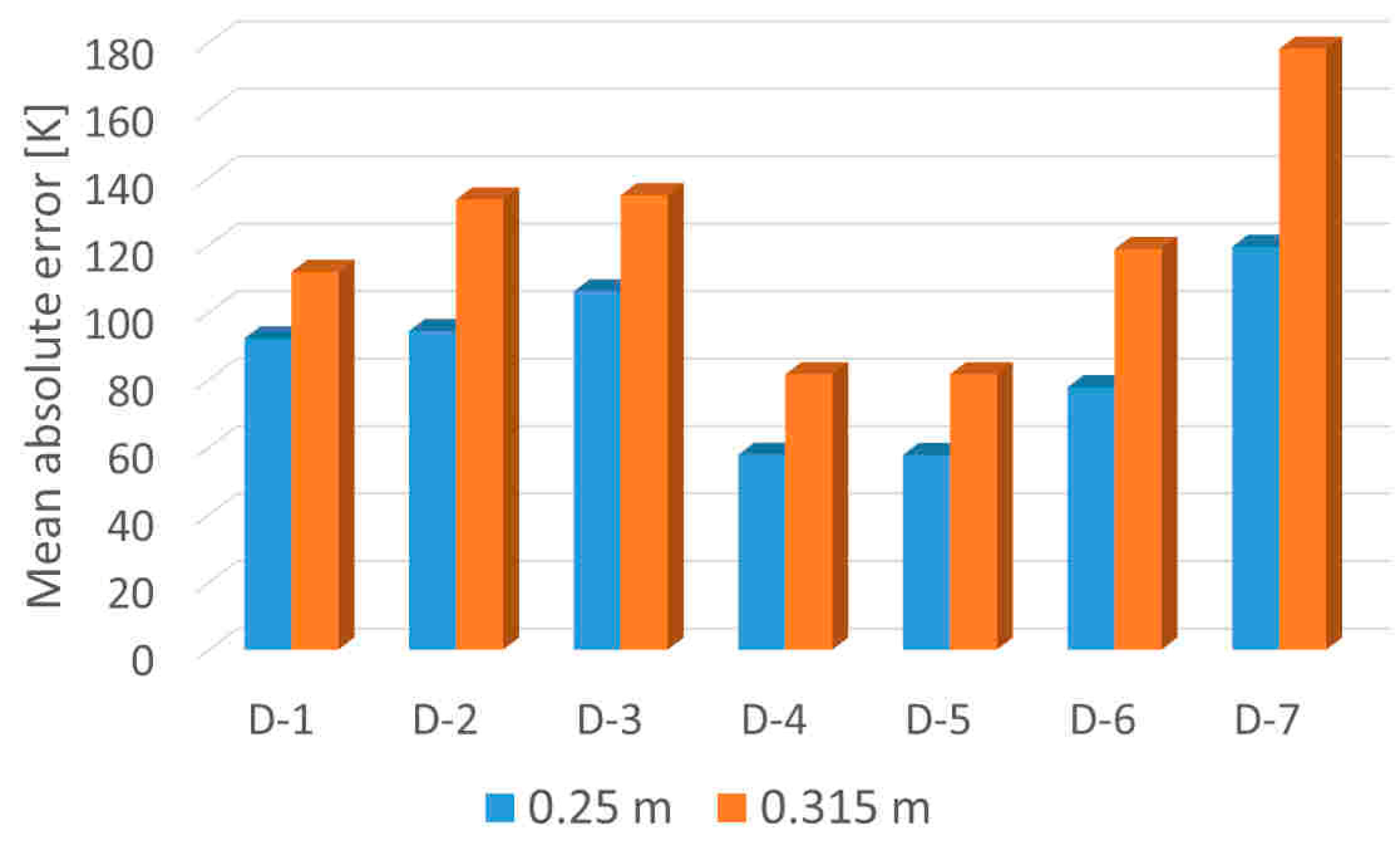
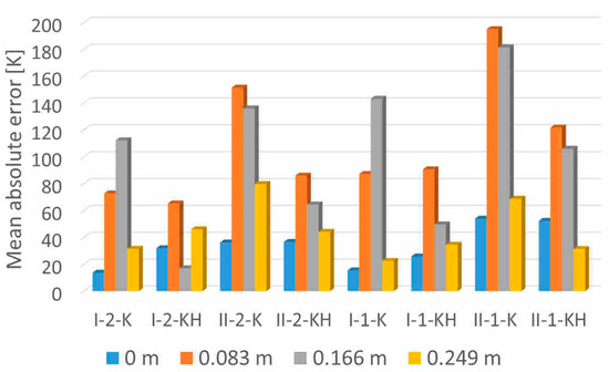
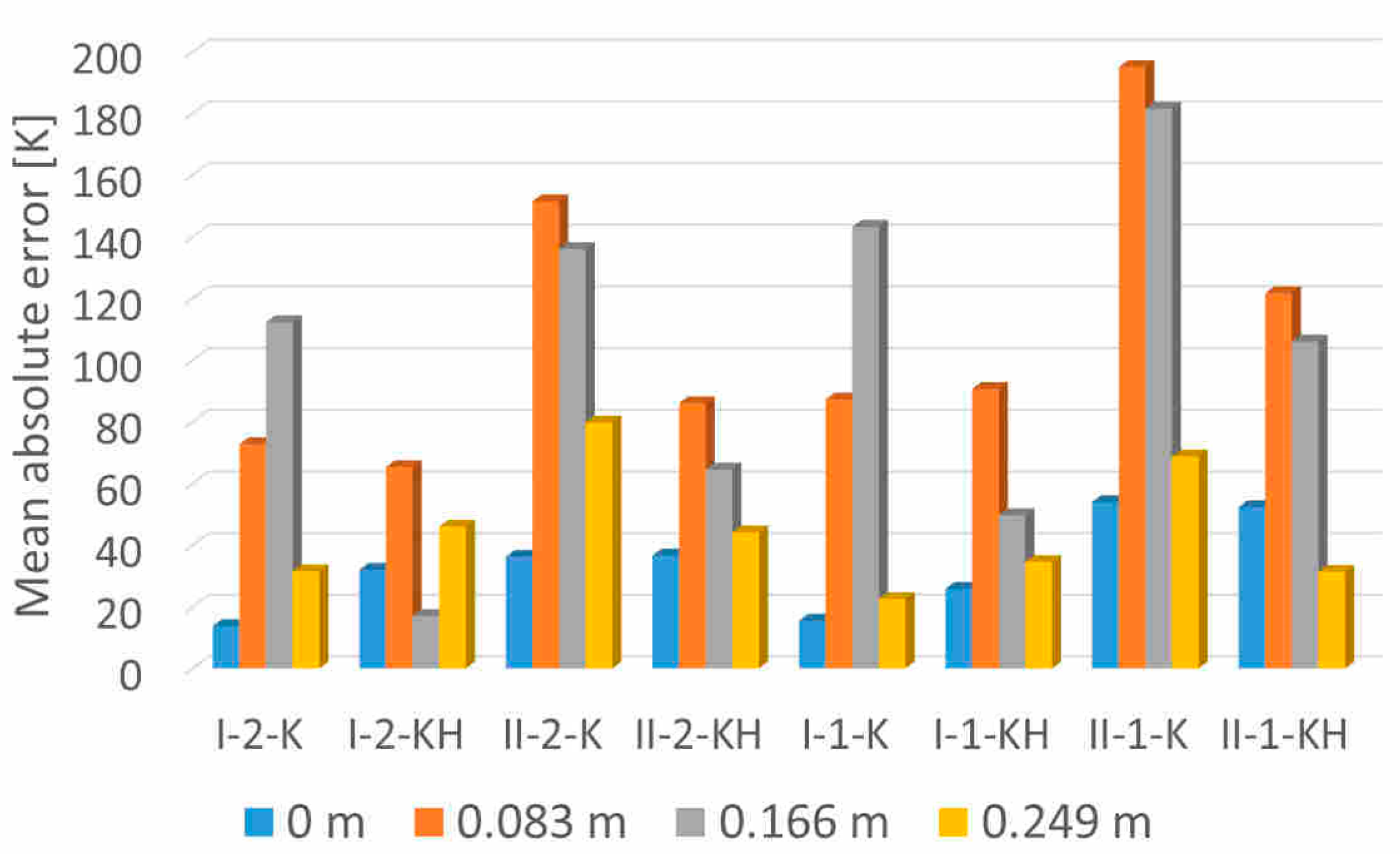
The values of mean absolute errors for individual domains were presented in Figure 4.
Figure 4.
The mean absolute errors for domains, for the two considered measurement heights, a rotational speed of 47,110 rpm and kerosene–hydrogen co-combustion.
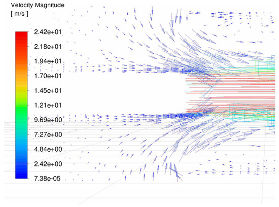
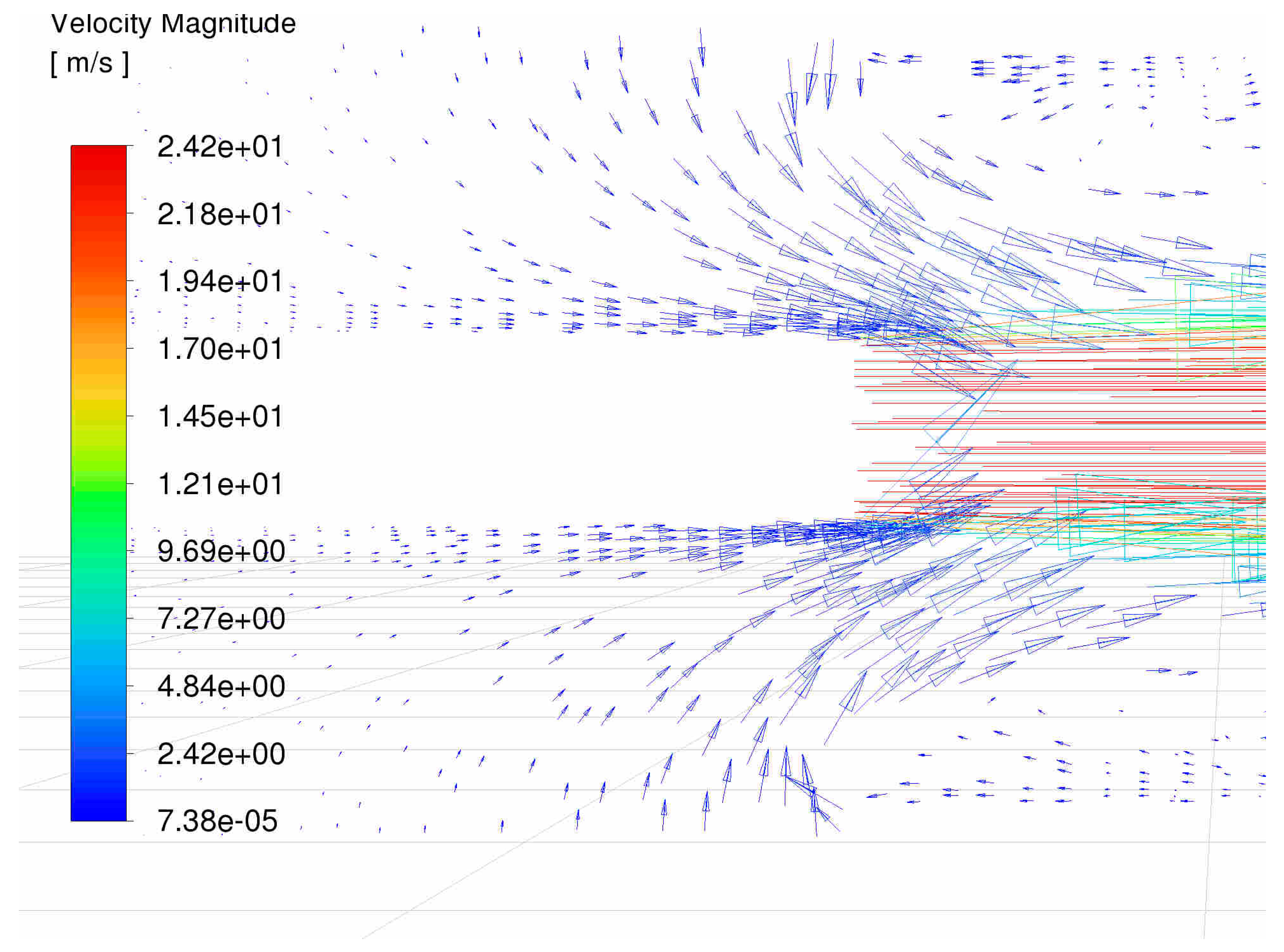
The largest errors with respect to experimental values occurred for domain D-1, and the smallest for domain D-4. Of these defined cases, only two were selected for further, more detailed, and fundamental research analysis. For variant 2, increasing the domain size led to increasingly smaller mean absolute errors. In variant 1, the presence of additional space outside the gap (D-7) increased the mean absolute error. It is worth noting that in domain D-3 the turbulence intensity had the lowest value, equal to 215. However, for domain D-4 much larger mean absolute errors occurred. For the domain variant including the gap, an inlet-air pressure inlet with ambient pressure (101,325 Pa) was used. Turbulence was left at the default settings: Turbulent Intensity = 5% and Turbulent Viscousity Ratio = 10. Analysis of the simulations taking into account the gap showed that the separated external area around the gap causes air to be directed into the container during engine operation, Figure 5. The presence of a gap without the external area, but using the inlet condition, does not account for this phenomenon. However, vertical flows are observed from the inside of the gap. Flows with different directions are observed in the corner of the container. In the simulation, both in domain 7 and domain 6, there are no back flows near the gap. A different image of the velocity distribution is presented by the simulation for domain 4. The visible flow directions near the gap are oriented towards the main stream and the container outlet. Ultimately, domains D-4 and D-6 were selected for further calculations. For domains 6 and 7, the first case was selected as variant 1 despite obtaining a higher turbulence intensity value. The reason for this choice was the temperature results, which contained significantly larger errors compared to domain 6.
Figure 5.
Velocity distribution—domain 7 (variant 1).
In the comparison of the SST k–ω and Realizable k-ε models, the same regions were analyzed for Variant 2, i.e., control points at distances of 0.25 m and 0.315 m from the container wall. Calculations were also performed for a speed of 47,110 rpm in the kerosene–hydrogen co-combustion mode. Mean absolute errors were calculated for both regions. In the first case, for the Realizable k-ε model, this error was 93.8 K, which was 20.9 K greater than for the SST k–ω model. In the second case, for the Realizable k-ε model, the error was 122.6 K, which was 38.3 K greater than for the SST k–ω model. The reason for this may be that the Realizable k-ε model predicts temperature distributions in near-wall regions worse. The turbulence intensity for the SST k–ω model was equal to 289, while for the Realizable k-ε it was 280. The analysis results showed that the SST k–ω model better predicted the temperature field and was therefore used in the further part of the study.
4. Results
The analysis of the results included a comparison of experimental measurements and the results of numerical calculations. Considering the two domain variants under consideration, parameters such as total pressure, temperature, and turbulence intensity were analyzed. In each case, speeds of 31,630 rpm and 47,110 rpm were considered, both in the kerosene combustion mode and in the kerosene and hydrogen co-combustion mode. The presented figures of the distributions of selected parameters inside the container primarily concern variant 2, for which the calculation results differed significantly less from the experimental results. This was described in Section 4.4.
4.1. Discussion Related to the Total Pressure Distribution
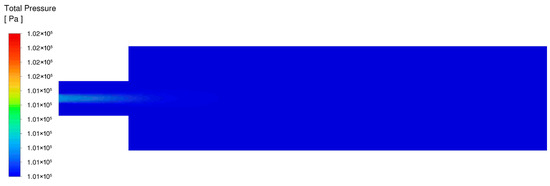
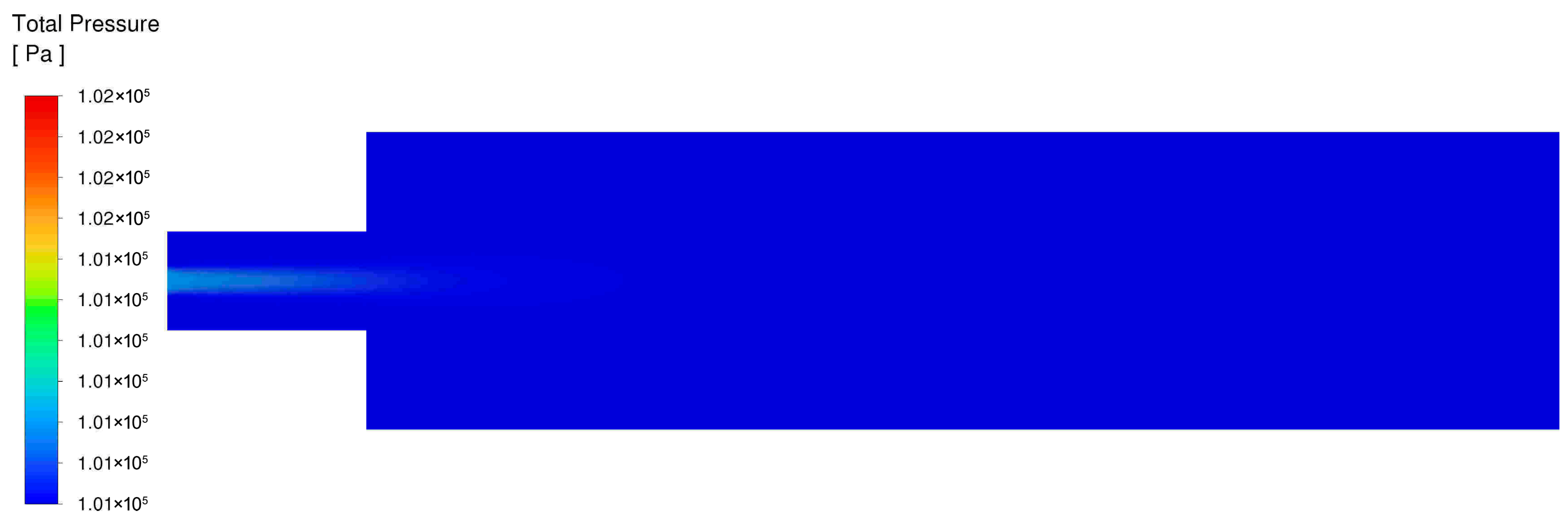
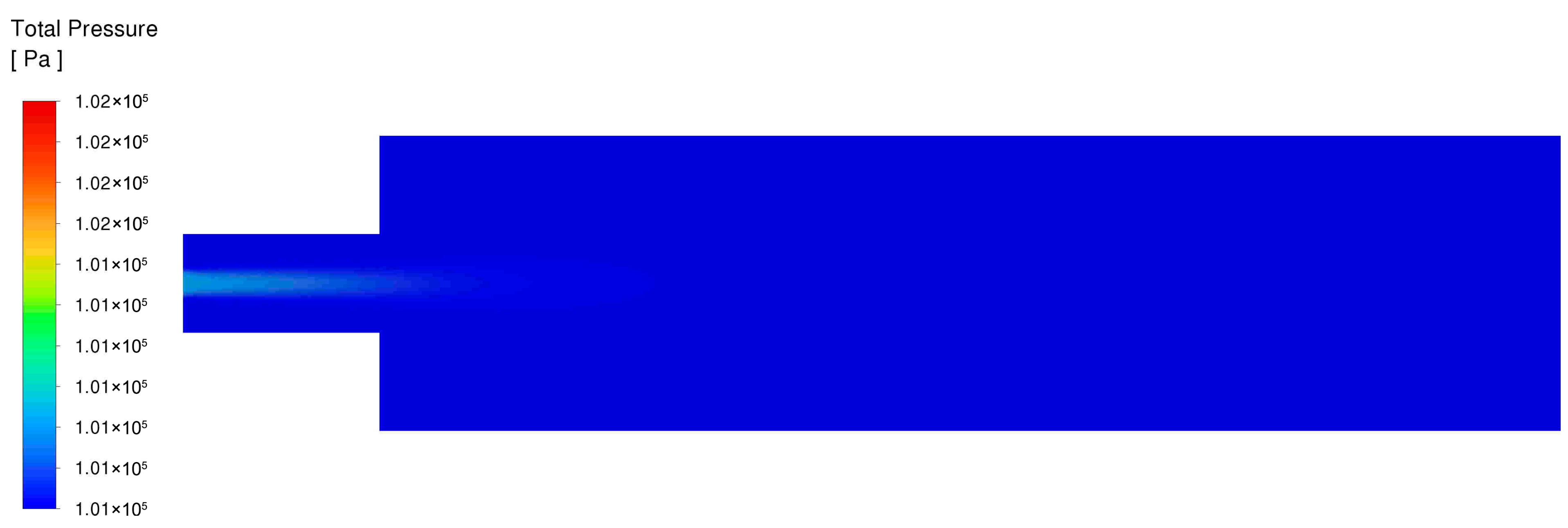
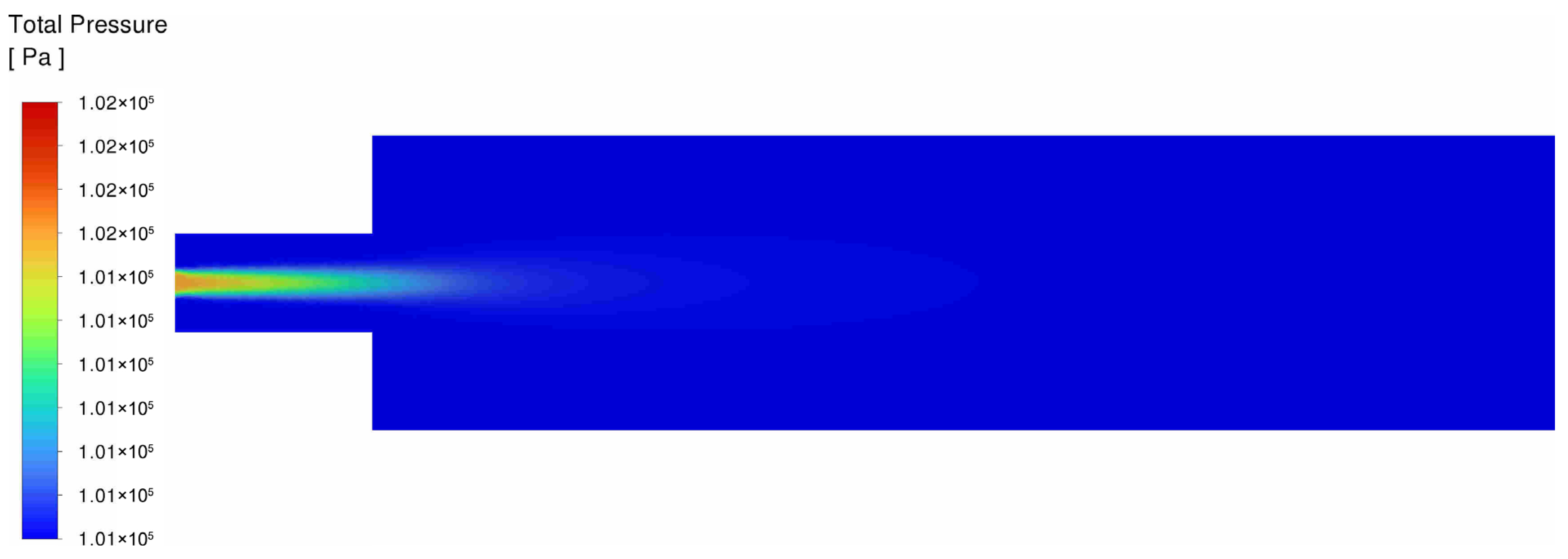
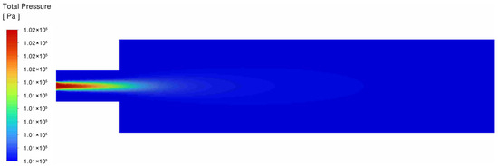
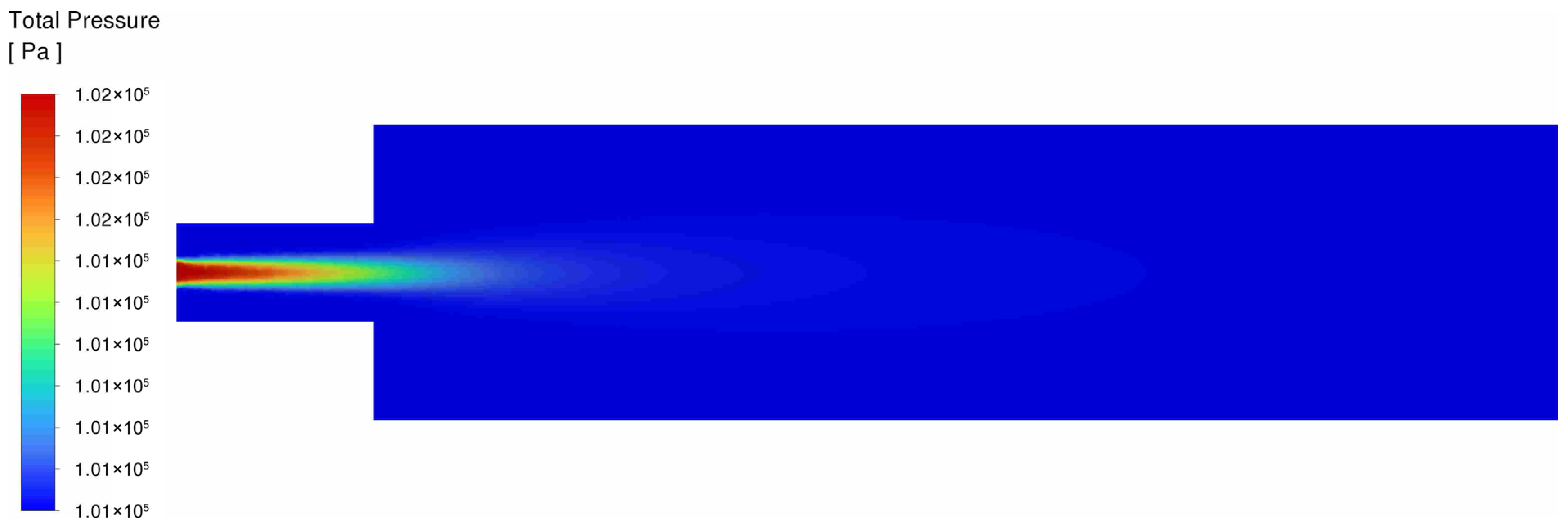
Combustion of a kerosene and hydrogen mixture generates a smaller area of total pressure with higher values. However, the maximum value is observed for kerosene–hydrogen co-combustion, at 31,630 rpm, at 101,388 Pa. This is an increase of 6 Pa compared to engine operation, where only kerosene is burned. The results for 47,110 rpm present a similar pattern. In this case, however, the gradient values obtained were significantly larger. For kerosene combustion, the maximum total pressure value is 101,515 Pa, while for kerosene–hydrogen co-combustion it is 101,604 Pa. For this rotational speed, the distribution area of this parameter is more similar, although the pressure gradients are stronger. The changes described above concern the domain for variant 2. The total pressure distribution was presented in Figure 6, Figure 7, Figure 8 and Figure 9.
Figure 6.
The total pressure distribution behind the nozzle for a speed of 31,630 rpm during kerosene combustion.
Figure 7.
The total pressure distribution behind the nozzle for a speed of 31,630 rpm during kerosene and hydrogen combustion.
Figure 8.
The total pressure distribution behind the nozzle for a speed of 47,110 rpm during kerosene combustion.
Figure 9.
The total pressure distribution behind the nozzle for a speed of 47,110 rpm during kerosene and hydrogen combustion.
The results obtained for variant 1 differ significantly from those for variant 2. Including a gap in the domain resulted in increased pressure gradients, primarily in its immediate vicinity. At a speed of 31,630 rpm for kerosene combustion, the total pressure was 101,396 Pa, while for kerosene–hydrogen co-combustion it was 101,404 Pa. At a speed of 47,110 rpm, the total pressure was 101,560 Pa and 101,681 Pa, respectively. Pressure gradients result directly from the increased dynamic pressure. For variant 1, an increase in this parameter was observed for speeds of 31,630 rpm and 47,110 rpm during kerosene combustion by 25.4% and 13.7%, respectively, compared to variant 2. Similarly, for both rotational speeds during kerosene–hydrogen co-combustion, there was an increase of 24.6% and 13.9%.
4.2. Discussion Related to Temperature Distribution
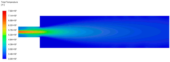
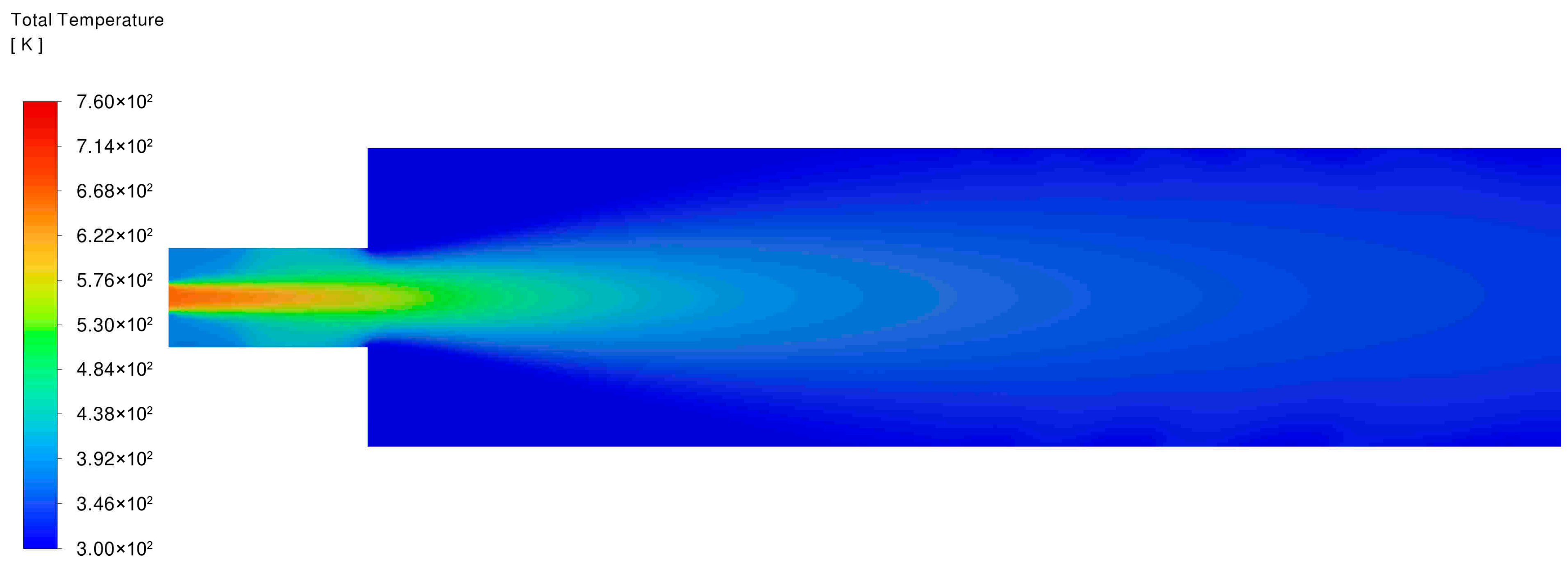
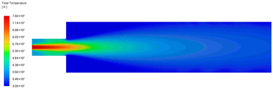
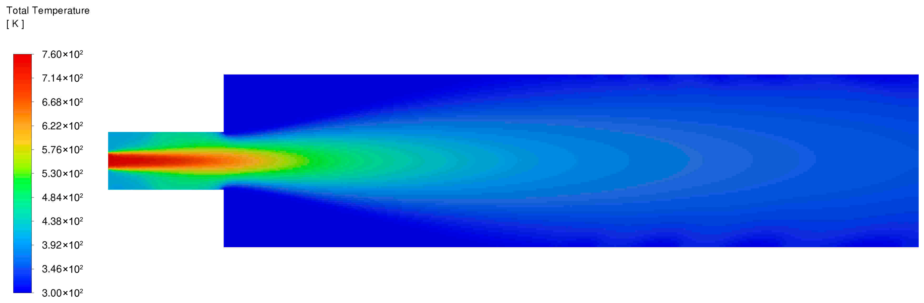
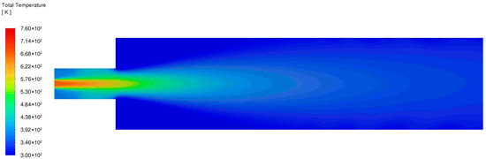
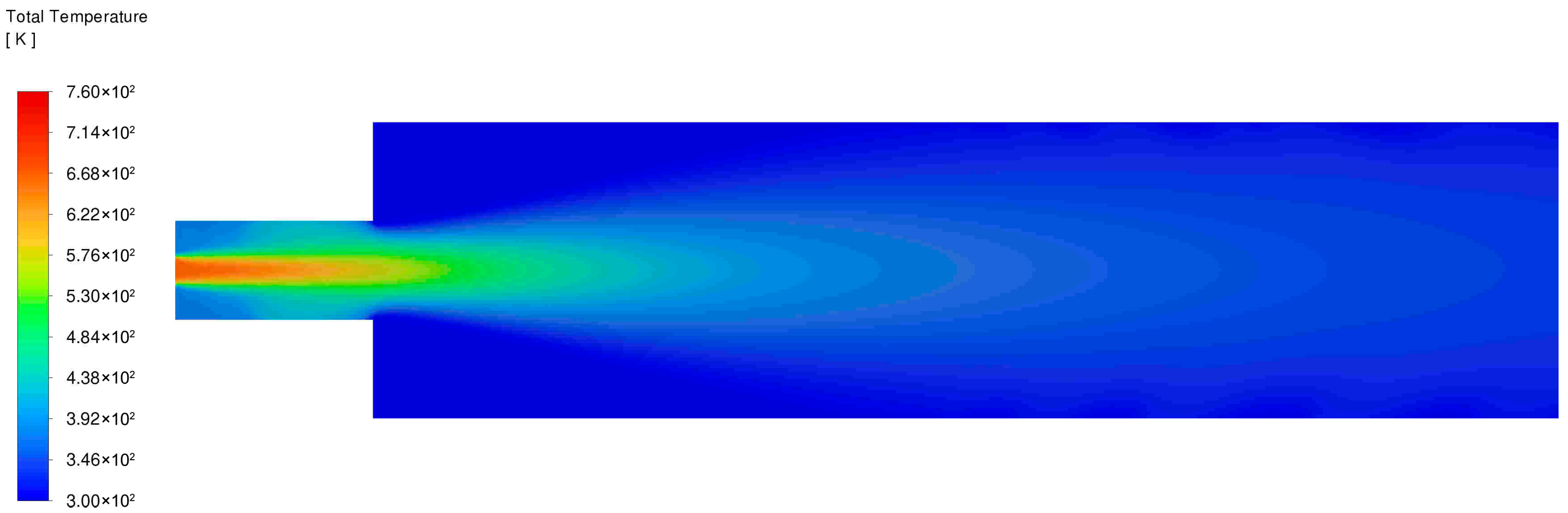
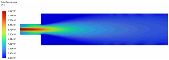
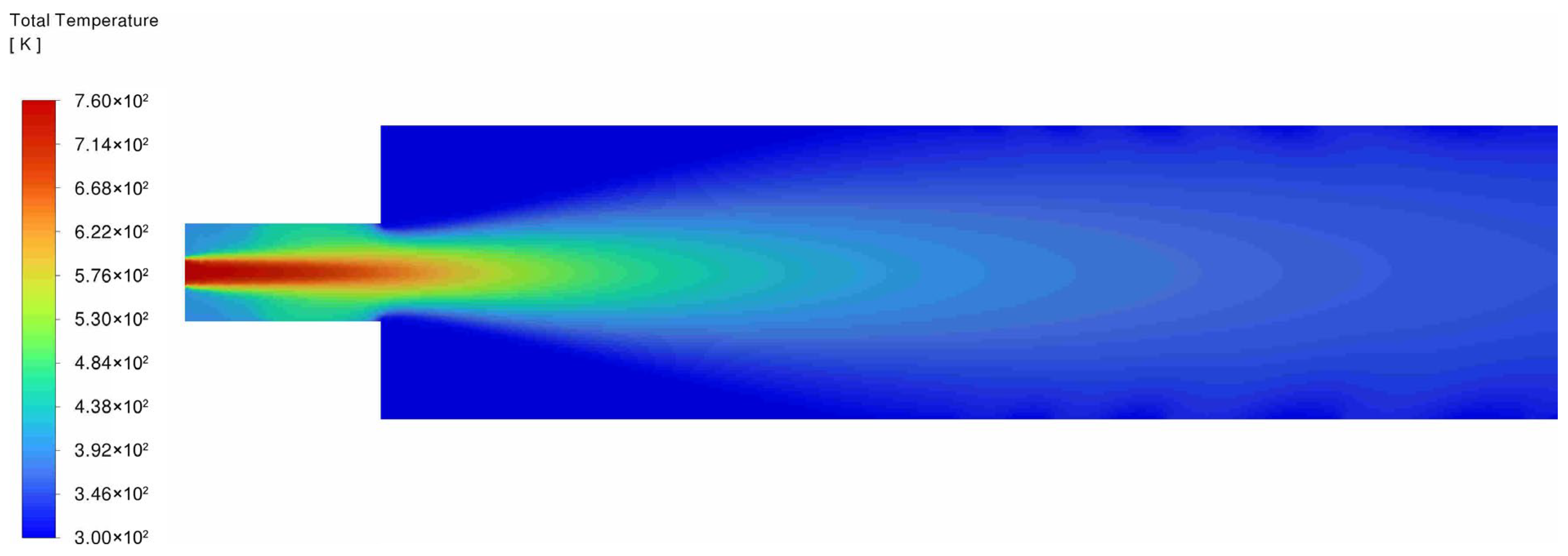
The shape and pattern of temperature gradient for both analysis variants are similar. The temperature field for variant 2 is presented in Figure 10, Figure 11, Figure 12 and Figure 13. However, the simulation showed that including the gap in the calculations leads to a significant temperature drop at the checkpoints. The maximum temperature for both variants, however, was the same. For the lower speed and kerosene combustion, it was 650 K, and for kerosene and hydrogen combustion, it was 750 K. For the higher speed and kerosene combustion, the temperature was 660 K, and for kerosene and hydrogen combustion, it was 760 K.
Figure 10.
The temperature distribution behind the nozzle for a speed of 31,630 rpm during kerosene combustion.
Figure 11.
The temperature distribution behind the nozzle for a speed of 31,630 rpm during kerosene and hydrogen combustion.
Figure 12.
The temperature distribution behind the nozzle for a speed of 47,110 rpm during kerosene combustion.
Figure 13.
The temperature distribution behind the nozzle for a speed of 47,110 rpm during kerosene and hydrogen combustion.
The analysis showed that in both variants, there are checkpoints where the temperature differs only slightly or not at all from the experimentally measured values. There are also points where the temperature gradients were very large. Examining the area halfway up the container at a speed of 31,630 rpm, larger temperature gradients appear much more frequently during kerosene–hydrogen co-combustion for both variants considered. A complete temperature comparison for this case was presented in Table 5.
Table 5.
The temperature comparison at altitude checkpoints (0.25 m container height) for a rotational speed of 31,630 rpm.
The results are similar for a speed of 47,110 rpm. For this case, the full temperature summary was provided in Table 6. For both the lower and higher speeds, the solution approximated using variant 2 proved to be closer to the actual measured results.
Table 6.
The temperature comparison at altitude checkpoints (0.25 m container height) for a rotational speed of 47,110 rpm.
Comparing the results at the control points in the upper plane (0.315 m), both for lower and higher speeds, they are similar to those at the midpoint of the container. All temperatures were presented in Table 7 and Table 8.
Table 7.
The temperature comparison at altitude checkpoints (0.315 m container height) for a rotational speed of 31,630 rpm.
Table 8.
The temperature comparison at altitude checkpoints (0.315 m container height) for a rotational speed of 47,110 rpm.
The largest differences between the calculated and measured values at the same points occur at a distance of 0.083 m and 0.166 m. This applies to both considered analysis variants.
4.3. Discussion Related to Turbulence Intensity
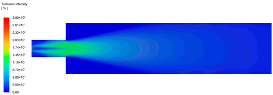
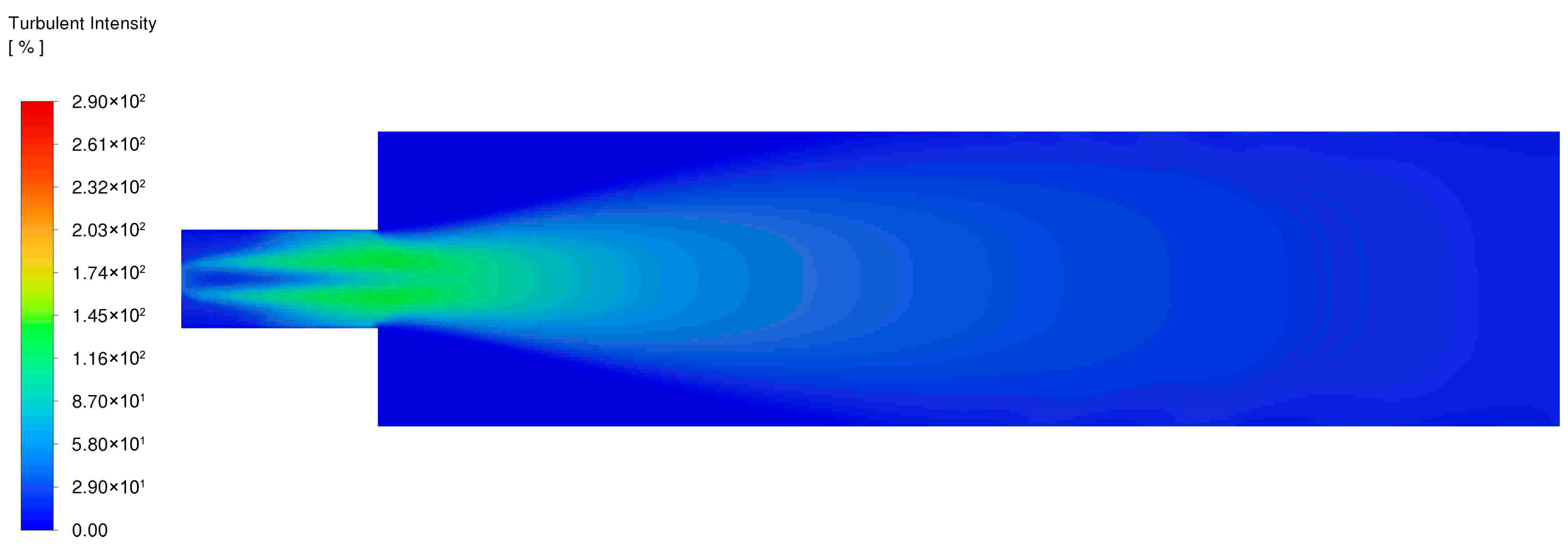
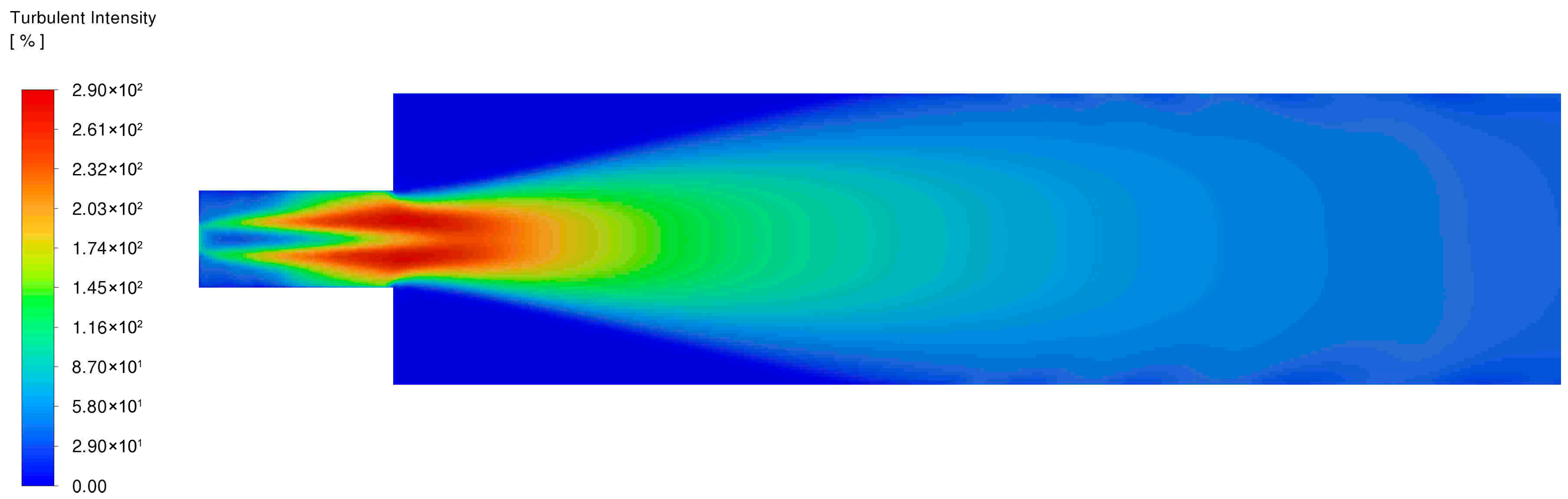
The next parameter examined in the analysis was turbulence intensity. The distribution field of this parameter for both speeds was presented in Figure 14, Figure 15, Figure 16 and Figure 17. A turbulence intensity below 1% indicates that the flow exhibits very weak characteristics of disturbed flow. The analysis showed that such a flow occurs near the walls, primarily in the front part of the container, i.e., on the engine nozzle side. This parameter increases slightly in the analysis that includes the gap, i.e., for variant 1.
Figure 14.
The turbulence intensity distribution behind the nozzle for a speed of 31,630 rpm during kerosene combustion.
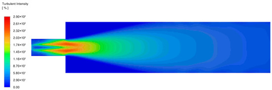
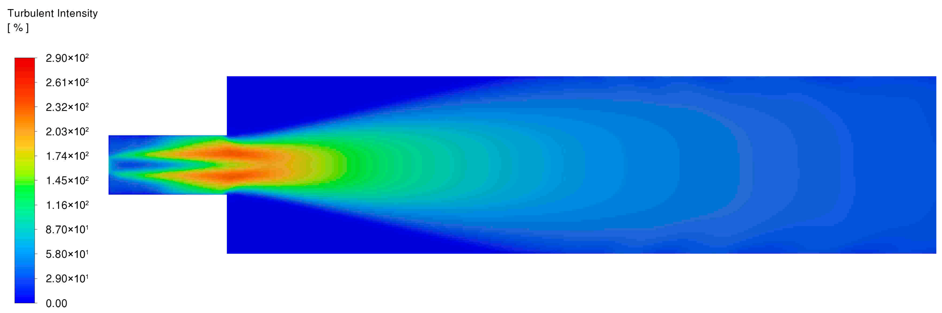
Figure 15.
The turbulence intensity distribution behind the nozzle for a speed of 31,630 rpm during kerosene and hydrogen combustion.
Figure 16.
The turbulence intensity distribution behind the nozzle for a speed of 47,110 rpm during kerosene combustion.
Figure 17.
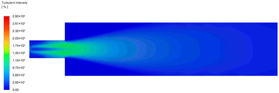
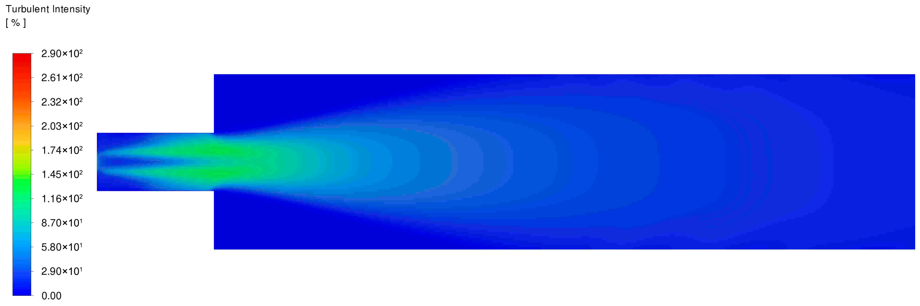
The turbulence intensity distribution behind the nozzle for a speed of 47,110 rpm during kerosene and hydrogen combustion.
The maximum turbulence intensity in analysis variant 1 at a speed of 31,630 rpm during kerosene combustion was 136% and for kerosene–hydrogen co-combustion 140%. For higher rotational speeds, this parameter was 244% for kerosene combustion and 300% for kerosene–hydrogen co-combustion. For analysis variant 2 at a lower speed, the turbulence intensity was 130% for kerosene combustion and 136% for kerosene–hydrogen co-combustion. For higher speeds, this parameter was 235% and 284%, respectively. Therefore, the use of the domain in variant 2 resulted in a decrease in this parameter for the lower and higher speeds in the case of using kerosene by 6% and 9%. Similarly, for the kerosene–hydrogen co-combustion, a decrease of 4% and 16% occurred, respectively.
4.4. Discussion Related to the Comparison of Experimental Measurements and Numerical Calculation Results
The temperature differences obtained at the checkpoints using numerical simulations were analyzed using several parameters. The first of these, also used during domain validation, was the mean absolute error. At a height of 0.25 m for variant 2, for kerosene, in the case of a speed of 31,630 rpm, the mean absolute error of all obtained results was 57.6 K, and for a speed of 47,110 rpm, 100.9 K. For the kerosene–hydrogen co-combustion, for a lower speed this parameter was 40.1 K, and for a higher speed 57.8 K. For variant 1, for kerosene, in the case of a speed of 31,630 rpm, the mean absolute error of all obtained results was 67.1 K, and for a speed of 47,110 rpm, 124.8 K. For the kerosene–hydrogen co-combustion, for a lower speed this parameter was 50.2 K, and for a higher speed 77.8 K.
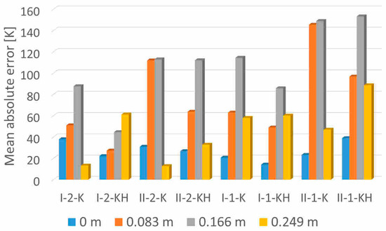
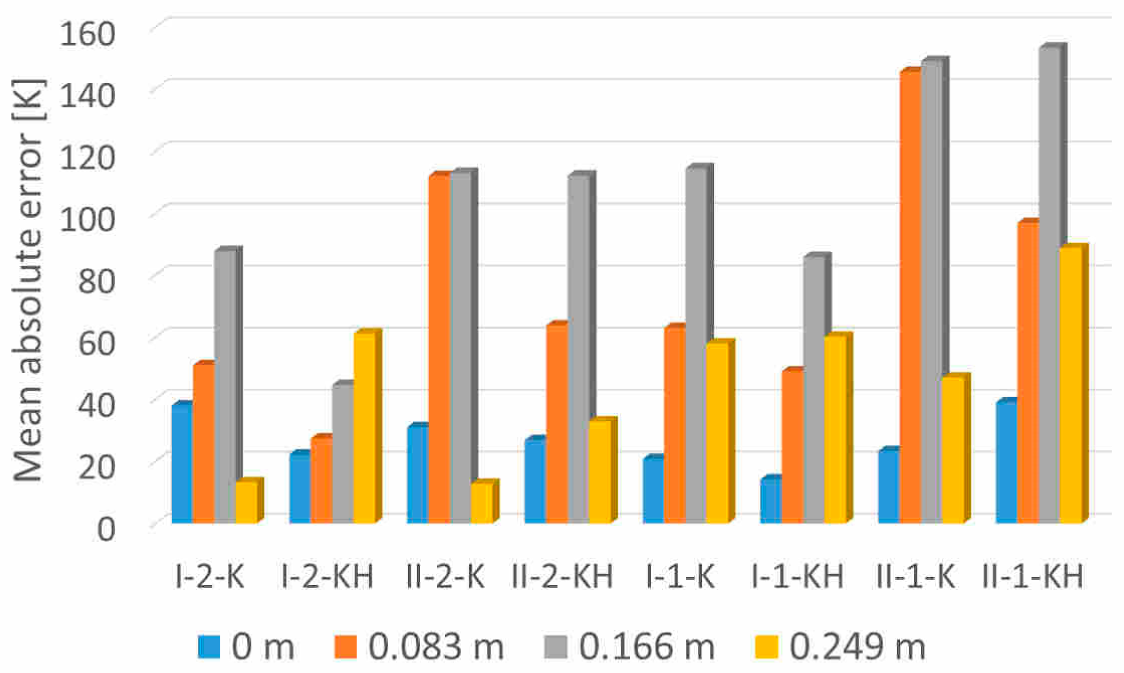
In the case of kerosene at a measurement height of 0.315 m for variant 2, at a speed of 31,630 rpm, the mean absolute error of all obtained results was 47.5 K, and for a speed of 47,110 rpm – 67.2 K. For the kerosene–hydrogen co-combustion, for a lower speed, this parameter was 38.8 K, and for a higher speed, 58.9 K. For variant 1, for kerosene, in the case of a speed of 31,630 rpm, the mean absolute error of all obtained results was 64.1 K, and for a speed of 47,110 rpm, 91.2 K. For the kerosene–hydrogen co-combustion, for a lower speed, this parameter was 52.3 K, and for a higher speed, 94.5 K. A more accurate distribution of this parameter in the context of the considered distances from the wall is presented in Figure 18 and Figure 19.
Figure 18.
The mean absolute error at the checkpoints at a height of 0.25 m: I—the rotational speed of 31,630 rpm, II—the rotational speed of 47,110 rpm, 2—variant 2, 1—variant 1, K—kerosene, KH—the kerosene–hydrogen.
Figure 19.
The mean absolute error at the checkpoints at a height of 0.315 m: I—the rotational speed of 31,630 rpm, II—the rotational speed of 47,110 rpm, 2—variant 2, 1—variant 1, K—kerosene, KH—the kerosene–hydrogen.
The distribution of the mean absolute error confirmed that its highest values occur in two intermediate areas, i.e., around 0.083 m and 0.166 m. For further evaluation of these two areas, the standard deviation was used, according to the following formula
where is the number of numbers in the set, is the difference between the measured and calculated temperature for both rotational speeds [K], is the arithmetic mean of all values [K].
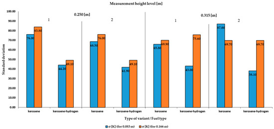
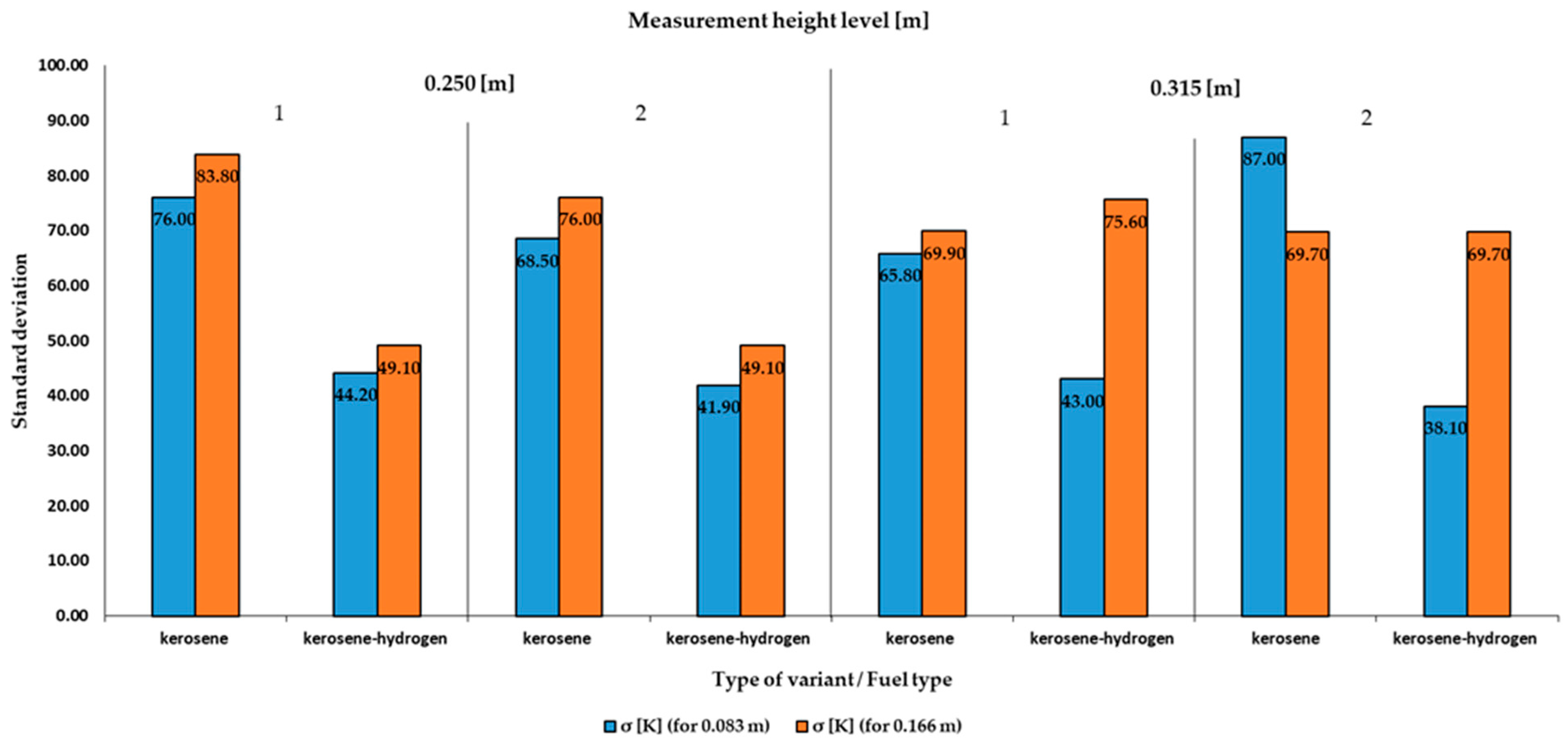
The analysis assumed that the standard deviation, as a certain component of uncertainty, can indirectly indicate the states of uncertainty at individual checkpoints. Therefore, at a height of 0.25 m in variant 2—for kerosene—the area with higher measurement uncertainty was located at a distance of approximately 0.166 m from the tank wall. For the kerosene–hydrogen co-combustion, this area had lower measurement uncertainty. For variant 1, in both cases, the greater measurement uncertainty was around a distance of 0.166 m from the container wall. At a height of 0.315 m, for both variants and both fuel types, the greater uncertainty was always around a distance of 0.166 m from the container wall. The standard deviation values were presented in Table 9. To improve clarity and provide a direct graphical interpretation of the deviations, the standard deviation values listed in Table 9 are additionally presented in Figure 19 in a bar-chart form. The figure enables a direct comparison of uncertainty levels between fuel types, measurement heights, and distances from the container wall. As shown in Figure 20, for both measurement heights (0.25 m and 0.315 m), the standard deviation is consistently higher at a distance of 0.166 m compared to 0.083 m, regardless of the variant considered. This trend confirms that the region located farther from the exhaust axis and closer to the container wall is characterized by stronger temperature fluctuations, which can be attributed to enhanced mixing, recirculation zones, and increased turbulence intensity. Furthermore, the graphical representation highlights that kerosene–hydrogen co-combustion generally exhibits lower standard deviation values at 0.083 m, indicating a more stable temperature field near the exhaust core, while at 0.166 m the differences between fuels become less pronounced, especially at the height of 0.315 m. This observation is consistent with the discussion above and confirms that uncertainty increases with distance from the jet core and with vertical elevation, where flow confinement effects dominate.
Table 9.
The standard deviation for the cases considered.
Figure 20.
Standard deviation of temperature measurements for kerosene and kerosene–hydrogen co-combustion at measurement heights of 0.25 m and 0.315 m, shown for two distances from the container wall (0.083 m and 0.166 m) and for both analyzed variants.
The errors related to the difference between the experimental results and the simulation results for variant 2 were presented in the form of RMSE in Table 10. It was calculated according to the formula
and in percentage
Table 10.
The RMSE in percent with respect to the mean experimental temperature values.
The RMSE values obtained in this work (9.5–22.8%) are within the ranges commonly reported for RANS-based temperature predictions in high-gradient jet exhaust environments. For miniature gas turbines, typical discrepancies between numerical and experimental temperature fields range an RMSE of 15% to 30%, as documented in recent small-scale turbine, afterburner and exhaust mixing studies. This confirms that the error levels observed here are consistent with limitations inherent to RANS modeling in strongly sheared, thermally stratified flows.
It should be noted that the very high turbulence intensity values obtained in the analysis (up to 300%) do not indicate physically unrealistic behavior but arise from the definition of turbulence intensity used in ANSYS Fluent. The parameter is computed as the ratio of the root-mean-square fluctuation of the velocity to the local mean velocity. In regions where the mean velocity drops sharply, such as in the shear layers surrounding the exhaust jet or inside recirculation zones, velocity fluctuations remain high while the mean velocity approaches low values. This combination can produce turbulence intensities well above 100%. Similar effects have been reported in confined exhaust jets, under expanded plumes and micro gas turbine mixing layers. The peaks observed in this study therefore correspond to strongly sheared, highly vortical regions at the jet boundary rather than to the core flow.
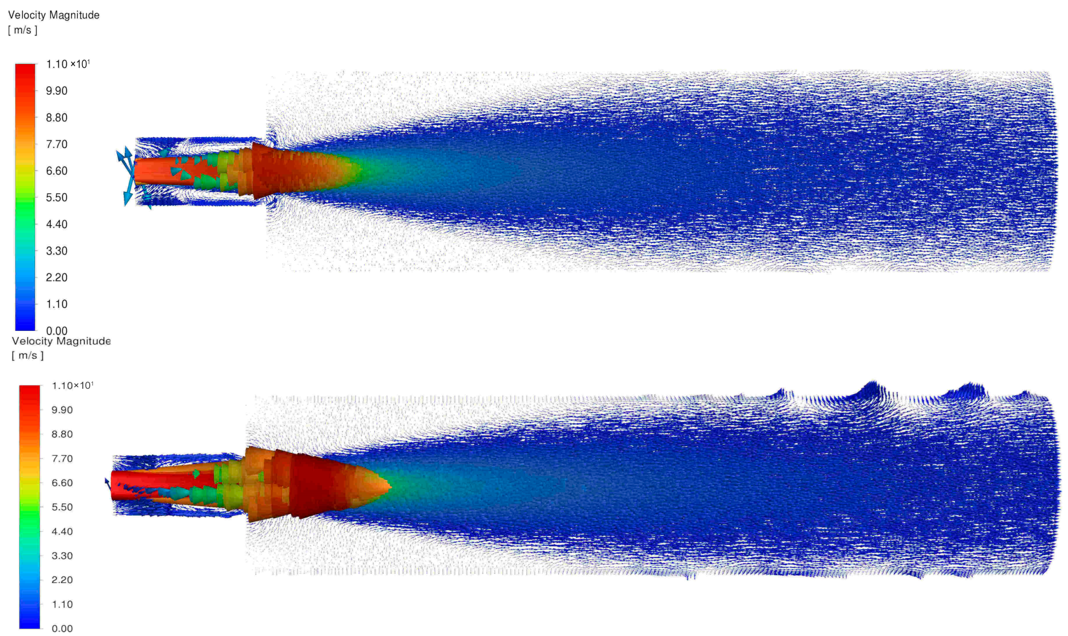
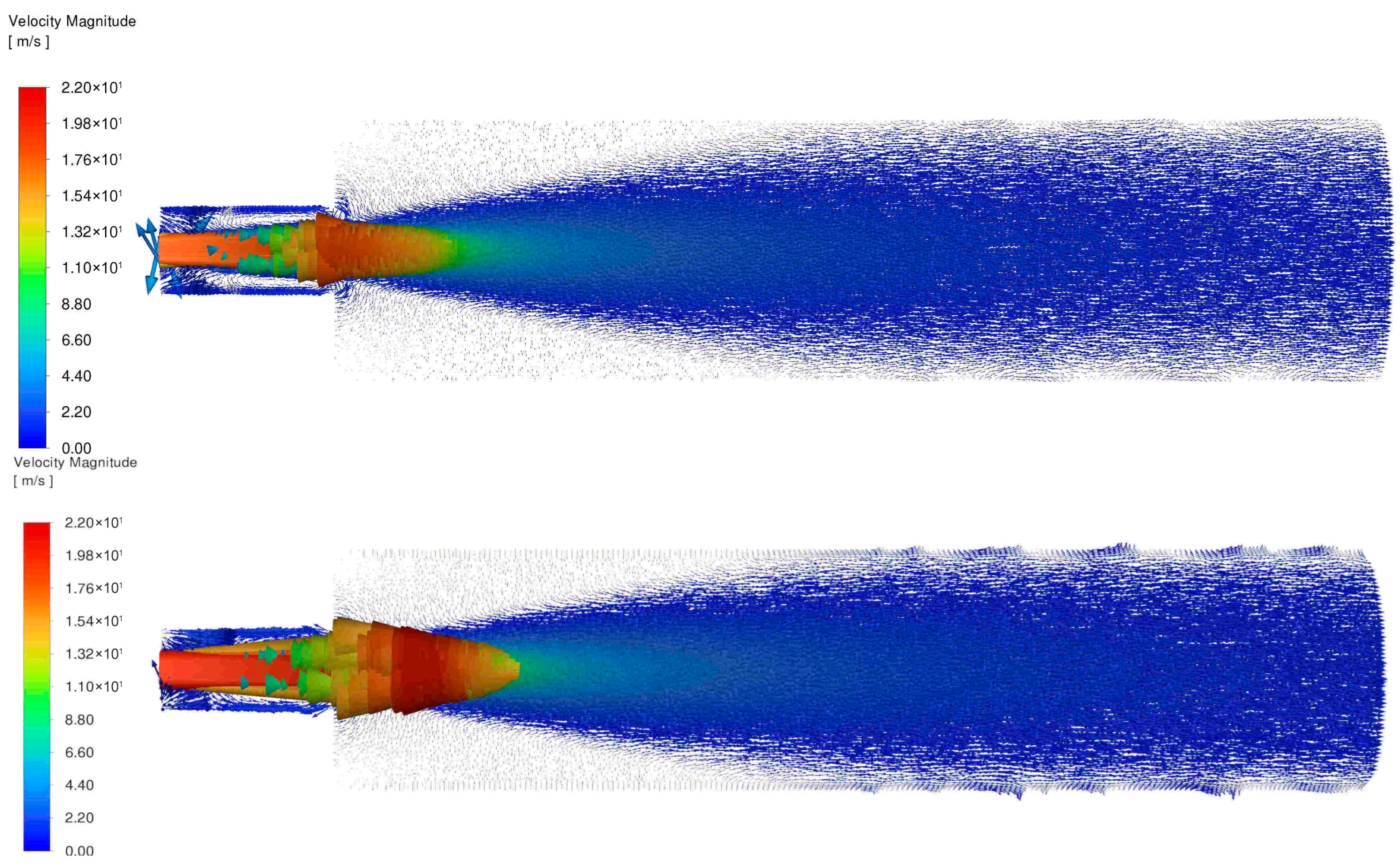
Figure 21 and Figure 22 present vector distributions of gas velocity in the container for both speed variants and fuel types used. The obtained results reveal differences in the form of local velocity development as well as the formation of vortex regions.
Figure 21.
The velocity distribution downstream of the nozzle for a speed of 31,630 rpm during kerosene combustion: variant 2 at the (top); variant 1 at the (bottom).
Figure 22.
The velocity distribution downstream of the nozzle for a speed of 47,110 rpm during kerosene and hydrogen combustion: variant 2 at the (top); variant 1 at the (bottom).
The same differences are observed for both lower and higher engine speeds. Local gas velocities outside the main exhaust stream are correspondingly higher for a speed of 47,110 rpm. Due to the limited space of the container on the engine side, a more intense gas flow is observed towards the exhaust stream, where the pressure is reduced. In this case, this is the only source of motion, apart from the particle motion in the exhaust cross-section. This leads to an increase in turbulent kinetic energy in the shear layers of the gas flow. In the presence of a gap, this flow is more pronounced. For variant 1, the maximum turbulent kinetic energy was 8.96 m2/s2, and for variant 2 it was 8.28 m2/s2.
4.5. Model Universality and Comparison with Literature
To assess the universality of the proposed CFD model and confirm its predictive reliability, a comparative analysis was conducted with published numerical and experimental investigations on miniature and small-scale turbojet engines operating under various fuel conditions. The goal was to determine whether the thermal and flow-field distributions obtained in this study are consistent with the general physical trends observed in similar engine configurations.
The obtained RMSE range (9.5–22.8%) aligns with the deviations typically reported for Reynolds-Averaged Navier–Stokes (RANS)-based simulations of small turbojet exhausts. Comparable levels of accuracy were documented by Badami et al. (2014) in their combined experimental–numerical study on small turbojets fueled by Jet-A and biofuel blends, where temperature prediction errors ranged between 10% and 25% depending on operating regime [27].
Similarly, Gao et al. (2014) investigated the flow and liner wall temperature field of a reverse-flow combustor for a miniature turbojet engine, validating CFD results against experimental data with an average temperature deviation of 12–20% [28]. Their findings confirmed that SST k–ω and standard k–ε models provide physically consistent turbulence structures downstream of the combustor, an observation mirrored by the present results.
In turn, Suchocki et al. (2014) analyzed the GTM-140 engine using a coupled non-premixed combustion and k–ε turbulence model, reporting exhaust temperatures between 870 and 950 K, which is consistent with the 890–1000 K outlet temperature range used as boundary conditions in the current simulation [29].
Furthermore, He et al. (2021) optimized a microturbojet combustor numerically and experimentally, demonstrating that turbulence intensity distributions within 200–300% correspond to flow instabilities localized in the shear layers—closely matching the present observations [30].
Finally, Brodzik et al. (2025) conducted a comprehensive thermomechanical analysis of the same GTM 400 MOD miniature turbojet engine using a coupled CFD–FEM framework, demonstrating that nozzle wall temperatures and stress distributions remained within experimentally verified material limits under both kerosene combustion and kerosene–hydrogen co-combustion conditions [13]. Their results confirmed the predictive robustness of steady-state RANS simulations implemented in ANSYS for evaluating thermal loads and structural response in hydrogen-assisted propulsion systems.
These findings are consistent with broader numerical investigations of alternative fuel combustion in turbojet engines. For instance, Alabas [31] showed that CFD-based modeling of hydrogen- and ammonia-enriched jet fuels yields realistic temperature levels and emission trends when appropriate boundary conditions and turbulence–radiation coupling are applied, further supporting the reliability of RANS-based approaches for hydrogen-containing fuel mixtures.
Moreover, the exhaust temperature ranges and operating conditions adopted in the present study align well with the characteristic parameters reported by Gieras [32] for miniature turbojet engines, who documented typical combustion chamber outlet temperatures and turbine loading levels for small-scale propulsion systems.
Taken together, these studies provide indirect yet consistent validation of the present numerical framework, confirming that the applied modeling assumptions lead to physically realistic predictions of thermal and mechanical behavior in miniature turbojet engines operating with both conventional and hydrogen-enriched fuels.
Taken together, these comparisons indicate that the present numerical model reproduces both the magnitude and spatial character of exhaust temperature fields and turbulence structures reported by other authors (Table 11). Hence, the model can be considered universal within the domain of small-scale turbojet exhaust simulations involving hydrocarbon and hydrogen-based fuels.
Table 11.
Comparison of study results and literature.
5. Conclusions
This study investigated the exhaust flow downstream of a GTM 400 MOD miniature turbojet engine operating under kerosene and kerosene–hydrogen co-combustion conditions. The primary objective was to assess the influence of geometric confinement and fuel composition on the thermal and flow characteristics of the exhaust jet and to verify whether a simplified numerical approach can reliably reproduce experimentally observed temperature fields.
The applied methodology combined experimental temperature measurements with steady-state CFD simulations performed using the SST k–ω turbulence model. Two numerical domain configurations were analyzed: one including the physical gap between the exhaust nozzle and the container (Variant 1) and one neglecting this gap (Variant 2). Model validation was conducted using temperature measurements collected at multiple distances from the exhaust axis and container wall, enabling quantitative assessment through normalized RMSE values.
The results demonstrated that the largest temperature deviations occurred in regions characterized by intensified turbulence and mixing, particularly at intermediate distances from the container wall. The highest turbulence intensities were observed for kerosene–hydrogen co-combustion at higher rotational speeds, reaching approximately 300% in Variant 1 and 284% in Variant 2. The analysis further showed that the simplified configuration without the gap (Variant 2) provided better agreement with experimental data, yielding RMSE values in the range of 9.5–22.8%, which is consistent with accuracy levels reported for RANS-based simulations of confined exhaust flows.
The scientific contribution of this work lies in demonstrating that the temperature field downstream of a miniature turbojet exhaust nozzle can be accurately reproduced without explicitly modeling the combustion process, provided that experimentally derived boundary conditions are applied. Additionally, the study quantifies the effect of geometric confinement on flow and temperature distributions and confirms, through comparison with independent experimental and numerical studies, the robustness and universality of the adopted numerical framework for small-scale turbojet exhaust analysis.
From an application perspective, the developed and validated model can be used for the thermomechanical assessment of miniature turbojet nozzles, optimization of confined exhaust and test chamber geometries, and preliminary evaluation of hydrogen-assisted combustion concepts. The approach is particularly suited for low- and medium-speed operating regimes, where reliable prediction of downstream temperature fields is required without excessive computational cost.
Author Contributions
Conceptualization, Ł.B. and B.C.; Methodology, Ł.B., B.C. and G.C.; Software, Ł.B. and B.C.; Validation, Ł.B., B.C., Ł.S., D.S. and G.C.; Formal analysis, Ł.B. and G.C.; Investigation, Ł.B.; Resources, Ł.B.; Data curation, Ł.B.; Writing—original draft preparation, Ł.B., B.C. and Ł.S.; Writing, review and editing, Ł.B., B.C., Ł.S. and G.C.; Visualization, Ł.B. and D.S.; Supervision, Ł.B. and G.C.; Project administration, Ł.B. and B.C.; Funding acquisition, Ł.B. and B.C. All authors have read and agreed to the published version of the manuscript.
Funding
This research was funded by the Polish Ministry of Science and Higher Education and the Poznan University of Technology’s financial resources for statutory activity. Grant numbers 0712/SBAD/5297 and 0712/SBAD/5298.
Data Availability Statement
The original contributions presented in this study are included in the article. Further inquiries can be directed to the corresponding authors.
Conflicts of Interest
The authors declare no conflicts of interest.
Nomenclature
| diffusion coefficient | |
| radiative intensity | |
| turbulent length scale | |
| first mixing function | |
| second mixing function | |
| external force | |
| thermal conductivity coefficient | |
| number of numbers in the set | |
| scattering phase function | |
| rate of production of turbulent kinetic energy | |
| effective rate of production of turbulent kinetic energy | |
| Prandtl number | |
| rate of production of specific turbulent dissipation rate | |
| term describing the combustion reaction | |
| mean rate of deformation component | |
| temperature | |
| temperature measured during the experiment at the checkpoint | |
| temperature calculated during simulation at the checkpoint | |
| mean flow velocity | |
| cross-diffusion term | |
| constant | |
| concentration of the reacting substance | |
| specific heat | |
| specific turbulent kinetic energy | |
| refractive index | |
| coordinate | |
| unit vector | |
| time | |
| velocity | |
| direction | |
| direction | |
| CFD | Computational Fluid Dynamics |
| FEM | Finite Element Method |
| MAE | Mean Absolute Errors |
| RDC | Rotating Detonation Combustor |
| RMSE | Root Mean Square Error |
| TBCC | Turbine-Based Combined Cycle |
| TKE | Turbulent Kinetic Energy |
| TDR | Turbulent Diffusivity Ratio |
| constant | |
| constant | |
| constant | |
| standard deviation | |
| stress tensor | |
| Kronecker delta function | |
| extinction coefficient | |
| coefficient of absorption | |
| coefficient of scattering | |
| arithmetic mean | |
| effective viscosity of specific turbulent kinetic energy | |
| modified eddy viscosity | |
| effective viscosity of specific turbulent dissipation rate | |
| density | |
| diffusion constant | |
| diffusion constant | |
| solid angle | |
| specific turbulent dissipation rate |
References
- Varatharajulu Purgunan, G.R.; Stathopoulos, P. Performance and Exergy Analysis of TurboJet and TurboFan Configurations with Rotating Detonation Combustor. Int. J. Thermofluids 2024, 23, 100739. [Google Scholar] [CrossRef] [Scilit]
- Zhang, Y.; Xu, J.; Pan, R.; Li, Y.; Ma, Z.; Huang, S. Numerical Investigation of Short Takeoff and Landing Exhaust System Using Bypass Dual Throat Nozzle. Aerosp. Sci. Technol. 2023, 138, 108316. [Google Scholar] [CrossRef] [Scilit]
- Meng, Y.; Shi, J.; Zhou, L.; Wang, Z. Numerical Investigation on Flow Characteristics of Multi-Stream Supersonic Nozzle with Serpentine Configuration. Aerosp. Sci. Technol. 2024, 144, 108799. [Google Scholar] [CrossRef] [Scilit]
- He, P.; Yue, C.; Fan, Y. The Stable Combustion and Blowout Characteristics Investigation of the Water Injection Pre-Cooling on the Afterburners. Fuel 2025, 397, 135422. [Google Scholar] [CrossRef] [Scilit]
- Aygun, H.; Kirmizi, M.; Kilic, U.; Turan, O. Multi-Objective Optimization of a Small Turbojet Engine Energetic Performance. Energy 2023, 271, 126983. [Google Scholar] [CrossRef] [Scilit]
- Niszczota, P.; Gieras, M. Inlet Injection as an Alternative, Simplified Method of Hydrogen Application in a Miniature Gas Turbine. Appl. Therm. Eng. 2024, 257, 124175. [Google Scholar] [CrossRef] [Scilit]
- Ayaz, S.K.; Caliskan, H.; Altuntas, O. Environmental and Second Law Analysis of a Turbojet Engine Operating with Different Fuels. Energy 2023, 285, 129402. [Google Scholar] [CrossRef] [Scilit]
- Kang, J.; Song, F.; Chen, X.; Wu, Y.; Zhang, D.; Wang, J.; Yang, Z.; Pan, W.; Wang, Z. Performance Enhancement of Rotating Detonation Afterburner through Combined Injection Scheme. Acta Astronaut. 2025, 235, 639–652. [Google Scholar] [CrossRef] [Scilit]
- Wu, X.; Hu, X.; Xiang, X.; Lin, S.; You, J.; Tian, F. An Analysis Approach for Micro Gas Turbine Engine’s Performance by Experiment and Numerical Simulation. Case Stud. Therm. Eng. 2023, 49, 103305. [Google Scholar] [CrossRef] [Scilit]
- Zhang, K.; Yu, X.; Zhang, D.; Guo, J.; Qin, F. Evaluation of Multi-Mode Shared Combustor with Different Flame Holder Designs for an Innovative Turbo-Ramjet Combined Cycle Engine. Energy 2025, 323, 135875. [Google Scholar] [CrossRef] [Scilit]
- Xu, Y.; Deng, W.; Liu, X.; Xu, H.; Li, Z. Full Engine 3D Simulation Scheme Considering Rotor Motion for Turbojet Engine under Crosswind Conditions. Appl. Therm. Eng. 2025, 269, 125951. [Google Scholar] [CrossRef] [Scilit]
- Boretti, A. Towards Hydrogen Gas Turbine Engines Aviation: A Review of Production, Infrastructure, Storage, Aircraft Design and Combustion Technologies. Int. J. Hydrogen Energy 2024, 88, 279–288. [Google Scholar] [CrossRef] [Scilit]
- Brodzik, Ł.; Ciupek, B.; Frąckowiak, A.; Schroeder, D. Thermomechanical Analysis of the GTM 400 MOD Turbojet Engine Nozzle During Kerosene and Hydrogen Co-Combustion. Energies 2025, 18, 4382. [Google Scholar] [CrossRef] [Scilit]
- Bogoi, A.; Cican, G.; Gall, M.; Totu, A.; Crunțeanu, D.E.; Levențiu, C. Comparative Study of Noise Control in Micro Turbojet Engines with Chevron and Ejector Nozzles Through Statistical, Acoustic and Imaging Insight. Appl. Sci. 2025, 15, 394. [Google Scholar] [CrossRef] [Scilit]
- Catana, R.M.; Badea, G.P. Experimental Analysis on the Operating Line of Two Gas Turbine Engines by Testing with Different Exhaust Nozzle Geometries. Energies 2023, 16, 5627. [Google Scholar] [CrossRef] [Scilit]
- Villarreal-Valderrama, F.; Zambrano-Robledo, P.; Hernandez-Alcantara, D.; Amezquita-Brooks, L. Turbojet Thrust Augmentation through a Variable Exhaust Nozzle with Active Disturbance Rejection Control. Aerospace 2021, 8, 293. [Google Scholar] [CrossRef] [Scilit]
- Ciupek, B.; Brodzik, Ł.; Frąckowiak, A. Research on Carbon Footprint Reduction During Hydrogen Co-Combustion in a Turbojet Engine. Energies 2024, 17, 5397. [Google Scholar] [CrossRef] [Scilit]
- Mazumder, S.; Roy, S.P. Modeling Thermal Radiation in Combustion Environments: Progress and Challenges. Energies 2023, 16, 4250. [Google Scholar] [CrossRef] [Scilit]
- Beer, J.M. Methods for Calculating Radiative Heat Transfer from Flames in Combustors and Furnaces, Chapter 2 in Heat Transfer in Flames; Afgan, N.H., Beer, J.M., Eds.; Scripta Book Company: Washington, WA, USA, 1974. [Google Scholar]
- Prokopowicz, W.; Ciupek, B.; Maciąg, A.; Gajewski, T.; Sielicki, P.W. Advanced Spectral Diagnostics of Jet Engine Vibrations Using Non-Contact Laser Vibrometry and Fourier Methods. Energies 2025, 18, 4837. [Google Scholar] [CrossRef] [Scilit]
- Brodzik, Ł. Gas temperature distribution in the combustion chamber of a GTM400 MOD turbojet engine powered by JET A-1 Fuel and Hydrogen. Energies 2024, 17, 745. [Google Scholar] [CrossRef] [Scilit]
- Karim, M.M.; Rahman, M.M.; Alim, M.A. Performance of SST k–ω turbulence model for computation of viscous drag of axisymmetric underwater bodies. Int. J. Eng. 2011, 24, 2. [Google Scholar]
- Liu, J.; Guo, W.; Yin, M.; Xi, W.; Sunden, B. Flow and heat transfer characteristic of regenerative cooling channels using supercritical CO2 with circular tetrahedral lattice structures. Case Stud. Therm. Eng. 2025, 71, 106204. [Google Scholar] [CrossRef] [Scilit]
- Liu, J.; Guo, W.; Zhao, G.; Ma, J.; Xi, W.; Sunden, B. Study on Heat Transfer Characteristics of Supercritical CO2/n-decane Composite Double Triangular Regenerative Cooling for Scramjets. Aerosp. Sci. Technol. 2026, 172, 111725. [Google Scholar] [CrossRef] [Scilit]
- Goldberg, U.C.; Batten, P. A wall-distance-free version of the SST turbulence model. Eng. Appl. Comput. Fluid Mech. 2015, 9, 1. [Google Scholar] [CrossRef] [Scilit]
- Rocha, P.C.; Rocha, H.B.; Carneiro, F.M.; da Silva, M.V.; Bueno, A.V. k–ω (shear stress transport) turbulence model calibration: A case study on a small scale horizontal axis wind turbine. Energy 2013, 65, 412–418. [Google Scholar] [CrossRef] [Scilit]
- Badami, M.; Nuccio, P.; Pastrone, D.G.; Signoretto, A. Performance of a Small-Scale Turbojet Engine Fed with Traditional and Alternative Fuels. Energy Convers. Manag. 2014, 82, 219–228. [Google Scholar] [CrossRef] [Scilit]
- Gao, X.; Duan, F.; Lim, S.C.; Yip, M.S. Experimental and Numerical Study of Flow Structure and Liner Wall Temperature in Reverse Flow Combustor. In Proceedings of the 15th International Heat Transfer Conference (IHTC-15), Kyoto, Japan, 10–15 August 2014. [Google Scholar] [CrossRef] [Scilit]
- Suchocki, T.; Lampart, P.; Klonowicz, P. Numerical Investigation of a GTM-140 Turbojet Engine. J. KONES Powertrain Transp. 2014, 21, 331–338. [Google Scholar] [CrossRef] [Scilit]
- He, W.; Guo, Z.; Xu, S.; Jin, Y. Numerical and Experimental Investigations on Performance Optimization of a Microturbojet Engine Combustor. Int. J. Aerosp. Eng. 2021, 2021, 6616537. [Google Scholar] [CrossRef] [Scilit]
- Alabas, H.A. CFD study of jet fuel with ammonia—Hydrogen mixtures in a jet engine: Emissions and combustion characteristics analysis. Int. J. Hydrogen Energy 2025, 142, 140–150. [Google Scholar] [CrossRef] [Scilit]
- Gieras, M. Miniaturowe silniki turboodrzutowe; Wydawnictwo Politechniki Warszawskiej: Warszawa, Poland, 2016. [Google Scholar]

Disclaimer/Publisher’s Note: The statements, opinions and data contained in all publications are solely those of the individual author(s) and contributor(s) and not of MDPI and/or the editor(s). MDPI and/or the editor(s) disclaim responsibility for any injury to people or property resulting from any ideas, methods, instructions or products referred to in the content. |
© 2026 by the authors. Licensee MDPI, Basel, Switzerland. This article is an open access article distributed under the terms and conditions of the Creative Commons Attribution (CC BY) license.