Study, Modelling and Computing of Pressure Losses in GH₂ Pipelines ^†

Abstract

The Wallonia region of Belgium aims to transition to a modern hydrogen infrastructure. Given the relatively low density of hydrogen gas, it is important to understand its nature and behavior during transport through pipelines. This study aims to observe the pressure loss in pipelines due to surface roughness with H₂ and other singular losses to find a solution to minimize the amount of pressure loss that occurs during transportation. This study involves numerical methods and gas equation models to determine the pressure loss. This analysis includes the properties of hydrogen gas, the pipeline material used, the friction factor, pipeline efficiency, and other relevant properties of hydrogen and pipelines. To address this challenge, the study integrates numerical fluid dynamics methods with structural modelling of pipeline walls. It accounts for long-term friction effects, erosion over several years, radial pressure gradients (mixing pressure drop), acceleration effects, and gravity influences, considering the non-ideal behavior of gaseous hydrogen (GH2). This study provides a systematic comparison between AGA-based analytical models and CFD simulations using a scaled pipeline approach, enabling reliable estimation of pressure losses in long-distance hydrogen pipelines. The proposed methodology integrates scaling, numerical validation, and CFD simulation to compute pressure losses in a hydrogen pipeline.

1. Introduction

Hydrogen is integral to the green transition. This has led countries to focus on hydrogen solutions for a rapid transition to a low-carbon economy. The relevance of hydrogen as a future energy source arises from its outstanding capability to address the intersecting challenges of security, environmental concerns and sustainable development. As a very light element, hydrogen has significant implications for transportation via pipelines due to low molecular weight and high diffusivity, which make it efficient for movement in pipeline systems. However, hydrogen also presents challenges, such as leakage and material embrittlement [1,2]. This work examines the importance of hydrogen as an energy carrier, its physical and chemical properties, numerical modelling of hydrogen flow in pipelines, recent developments in flow experiment procedures, current issues related to the use of pipelines for hydrogen gas, and transport and solutions. Hydrogen transport involves various methods, including the use of pipelines, tank trucks, or carriers using gases such as ammonia. The main hydrogen storage method is high-pressure storage and transportation in using compressed gas containers. An additional efficient method for transporting hydrogen is through pipelines [3], which provide constant, large-scale transportation at a relatively low cost.

1.1. Literature Review

In the practical world, one of the potential ways to transport hydrogen gas is through natural gas pipelines. An example in the UK is Project H21, which uses the existing natural gas pipeline infrastructure to transport hydrogen. Any pipeline network comprises chains of distribution networks, such as gathering, transmission, distribution, service lines, and re-compression of H₂ gas pressure using compressors on transmission lines. Khan et al. [3] summarized that the choice of materials and their properties for pipelines play an important role. The author has pointed out high-strength steels (above 100 KSI), which are used in natural gas pipelines, are more susceptible to hydrogen embrittlement. Therefore, materials with low-strength steel are recommended for hydrogen pipelines. This study also explains the impact of the surface roughness of a material. The relationship between pipe roughness and pipe length is directly proportional; as the surface roughness increases, the pressure loss also increases along with the length of the hydrogen pipeline.

1.2. Existing Methods and Limitations

Hydrogen is being considered as a fuel of the future from an industrial perspective; however, the method of obtaining hydrogen is not the only issue faced by industries, but also its transportation and storage. One method of transporting hydrogen gas is by truck transportation, but this is effective only for relatively short distances and limited volumes. This limitation is the main reason industries focus on hydrogen transport through pipelines. Currently, natural gas pipelines can serve as a medium for hydrogen transport, as they are designed for long-distance transmission and operate at maximum operating pressure. Another advantage is the existence of a pipeline network. Utilizing this available infrastructure would be a good option; however, there are some disadvantages to using natural gas pipelines. Hydrogen can penetrate through the material of a natural gas pipeline, resulting in corrosion and hydrogen embrittlement. These characteristics make transporting hydrogen gas through natural gas pipelines challenging.

1.3. Objective

The focus of the current study is on transportation pipelines, which are used to transport hydrogen over long distances. In the process of hydrogen transmission, pressure loss is a major factor that limits the amount of hydrogen transportation. To minimize the effect of pressure drop, various factors must be considered, including pipeline length, diameter, material surface roughness, material choice for hydrogen gas transportation, friction factor, operating pressure value, volumetric flow rate and hydrogen gas properties. In addition, factors that cause pressure drops, such as leakage and safety valves, must also be considered because an unexplained drop is a sign of hydrogen release, which could lead to an explosion due to the highly flammable nature of hydrogen. To compute the pressure loss accurately, leakage and safety valves must be considered, as they provide a baseline if the actual pressure is lower than the calculated pressure to avoid an unexpected pressure drop.

In this study, mathematical modelling and CFD analysis were performed to calculate the pressure drops in a transportation pipeline carrying hydrogen gas at a fixed high volumetric flow rate and a pipeline distance of 100 km to observe the pressure drop value for different operating pressure values ranging from 50 to 120 bar [3]. For the purpose of this study, the inclusion of compression stations is omitted, given that the considered distance is assumed to be optimal and variations in elevations are not taken into account.

2. Materials and Methods

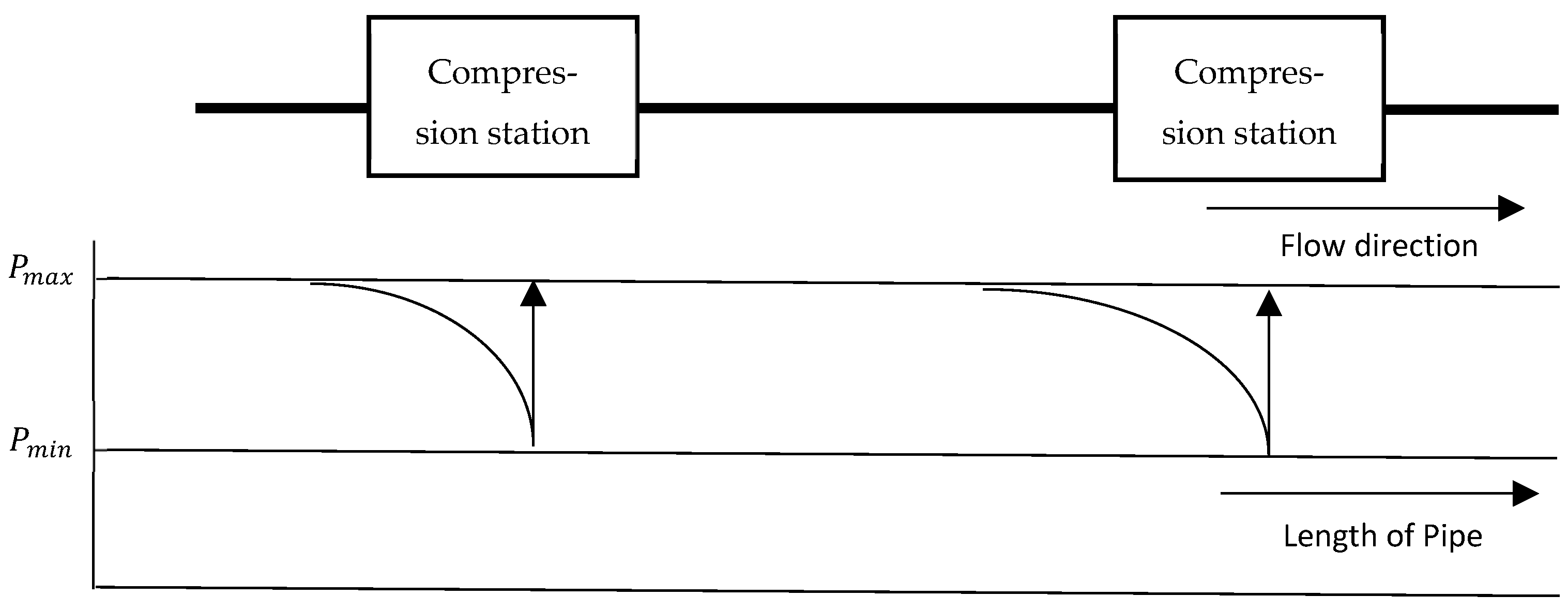
The transportation of hydrogen gas through pipelines is shown in Figure 1. The flow of hydrogen gas is due to the principle of pressure-difference-induced flow. The interaction between the viscosity of the gas and the friction with the pipe wall results in a pressure drop. As the velocity of the gas inside the pipeline increases, the pressure drop increases proportionally. To overcome the larger pressure drop, compression stations need to be installed at 80–100 km [4]. The functionality of the compressor station restores pressure losses when hydrogen gas needs to travel long distances. During hydrogen gas transport, it is very important to maintain gas velocity within the limit known as the erosional limit to avoid any catastrophic situations within the pipeline connections.

Pipelines can be made from a wide range of materials, which show relative contributions per distance by various types of gas. Carbon steel is an alloy commonly used in hydrogen gas transmission pipelines. The maximum hardness for hydrogen pipeline service should be approximately 22 HRC or 250 HB. The maximum hardness is the same as the maximum tensile strength. The maximum tensile strength should be approximately 800 MPa. Low-strength materials made of stainless steel are sometimes suggested for use in H2 pipelines [3,5]. In this study, API X52 material and its properties were used, as it is the most widely used material in pipelines, and the pressure loss calculation was based on the same material roughness values.

3. Method of Computing and Validation of Equation Model

To begin with, the computation of the pressure drop involves many available models. In this study, the American Gas Association (AGA) model was used [6,7]. This model includes surface roughness and pipeline efficiency factors inside, which have a direct influence on pressure loss. The other models are named as follows:

• Panhandle A Equation
• Panhandle B Equation
• Weymouth Equation
• General flow Equation

To calculate the pressure loss, the AGA (American Gas Association) Equation is given in Equation (1).

$$\mathrm{Q}=0.018\ast \left({\displaystyle \frac{T_s}{P_s}}\right)\ast \mathrm{E}\ast 4\ast {\log }_{10}\left({\displaystyle \frac{3.7\ast \mathrm{d}}{\mathsf{\epsilon }}}\right)\ast {\left({\displaystyle \frac{{\mathrm{P}}_1^2-{\mathrm{P}}_2^2}{\mathsf{\gamma }\ast \mathrm{L}\ast \mathrm{T}\mathrm{a}\mathrm{v}\mathrm{g}\ast \mathrm{Z}}}\right)}^{0.5}\ast {\mathrm{d}}^{2.5}$$

(1)

Q—Flow rate of gas at standard conditions (m³/s)

T_s—Standard H₂ temperature (K)

P_s—Standard H₂ pressure (bar)

E—Pipeline efficiency (typically between 0.8 and 1)

• −

  1 in the absence of field data (also for a new straight pipe with no diameter change)

  −

  0.95 for very good operating conditions, typically through the first 12–18 months

  −

  0.92 for average operating conditions

  −

  0.85 for unfavorable operating conditions

d—Internal diameter of pipeline (m)

P₁—Inlet H₂ pressure (bar)

P₂—Outlet H₂ pressure (bar)

$\mathsf{\gamma }$—relative density of H₂ (kg/m³)

L—Length of pipeline (km)

Z—Compressibility factor of H₂ gas (dimensionless)

$\mathsf{\epsilon }$—Absolute surface roughness of material (m)

$\mathsf{\gamma }$—Relative density of flowing gas for hydrogen (0.0696)

T_avg—Average temperature of H₂ gas (K)

The pipeline efficiency factor (E) measures the difference between real-world pipeline performance and the idealized conditions of gas flow. It accounts for additional losses due to real-world factors such as pipeline roughness, deposits, small fittings, and ageing, which are not considered in analytical calculations. The pipeline efficiency factor generally ranges from 0.8 to 1.0. The pipeline operates more efficiently under favorable conditions; conversely, lower efficiency indicates operation under unfavorable conditions. In this study, the efficiency is considered to be 1.0, as the case involves a straight pipe with a constant diameter along its length.

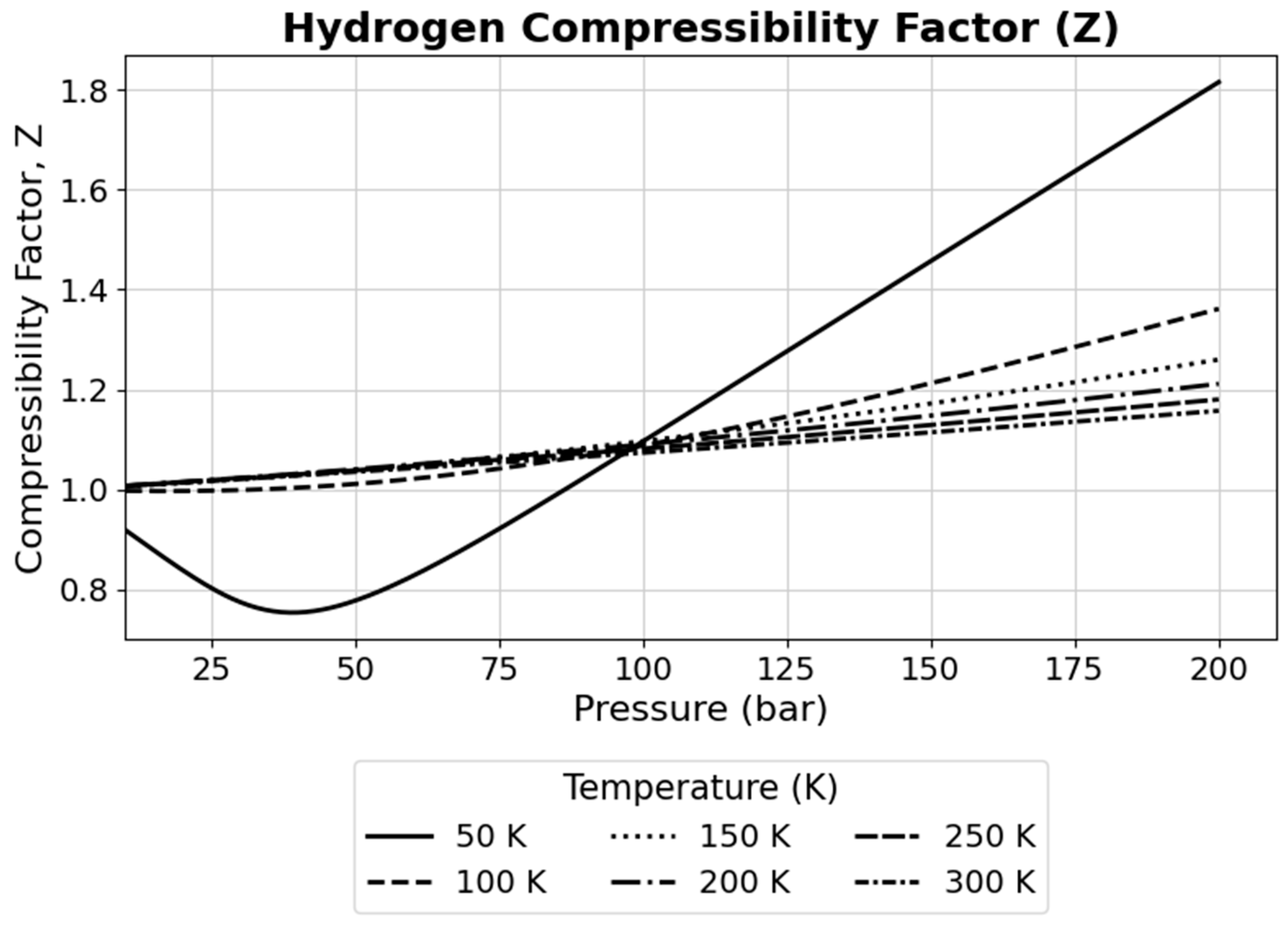
The compressibility of hydrogen is an intrinsic property that affects its transport and depends on temperature, as it is influenced by intermolecular forces. At low temperatures and high pressures, hydrogen tends to be non-ideal (Z > 1). With low kinetic energy, intermolecular repulsive forces become more pronounced, causing hydrogen to occupy more space than it would as an ideal gas. As temperature increases, the greater kinetic energy of hydrogen molecules overcomes intermolecular forces. Hence, it tends to act ideally, and its compressibility factor approaches (Z ≈ 1). The compressibility factor for hydrogen gas is shown in Figure 2.

The friction factor f was calculated using the Colebrook–White Equation (2):

$${\displaystyle \frac{1}{\sqrt{f}}}=-2log{\displaystyle \frac{2.51}{Re\sqrt{f}}}+{\displaystyle \frac{\epsilon }{3.7d}}$$

(2)

f—Friction factor (dimensionless)

$\epsilon$—Pipeline material roughness (m)

d—Internal diameter of pipeline (m)

R_e—Reynolds number

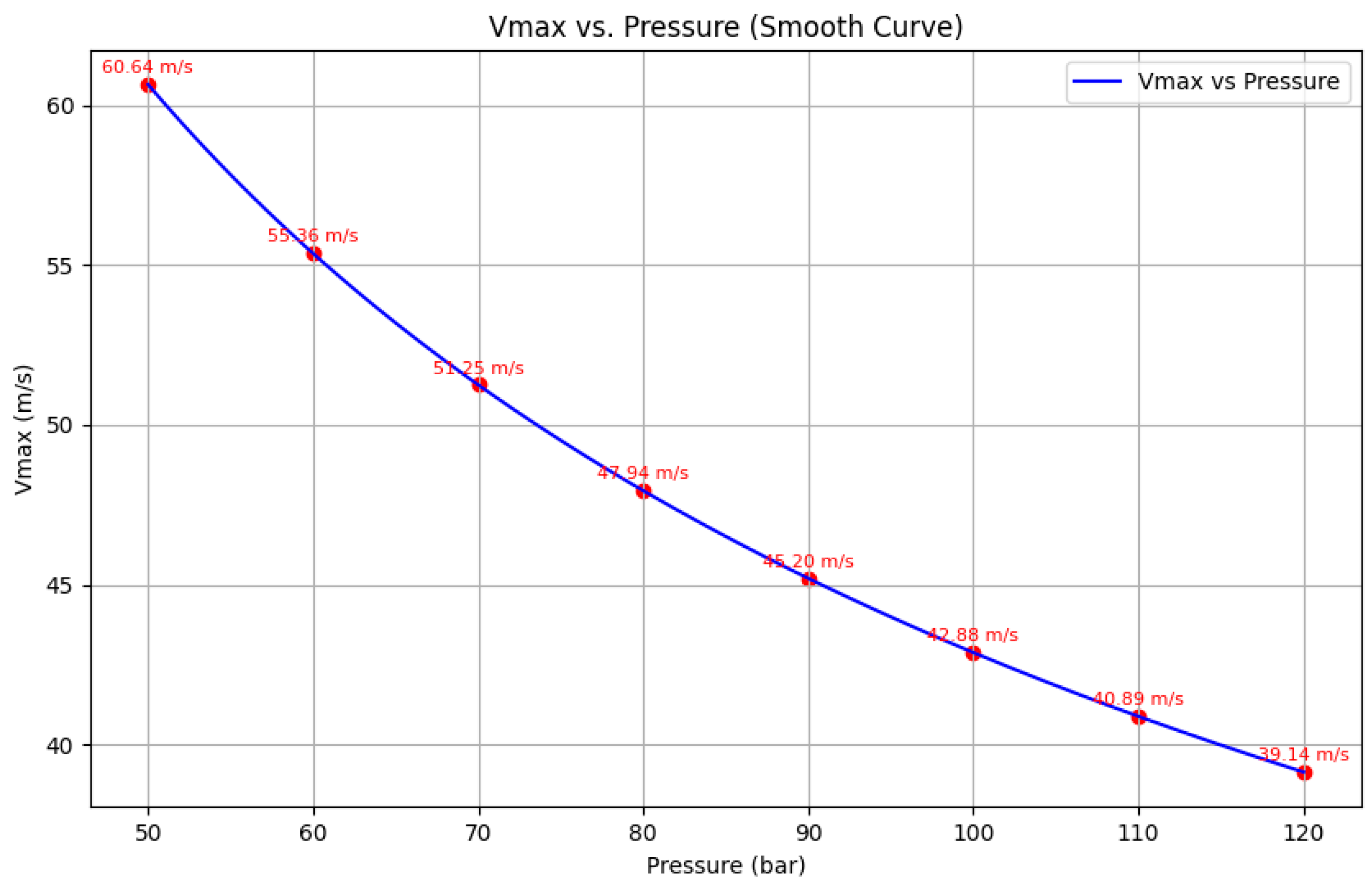
The erosional velocity represents the maximum velocity of gas moving through a pipeline. Higher velocities can result in pipe wall erosion over time. In AGA, the erosional velocity V_max is calculated using Equation (3) and shown in Figure 3:

$${\mathrm{V}}_{\mathrm{m}\mathrm{a}\mathrm{x}}=100\sqrt{0.05131{\displaystyle \frac{\mathrm{Z}\mathrm{R}\mathrm{T}}{\mathrm{G}\mathrm{P}}}}$$

(3)

V_max—Erosional velocity (m/s)

P—Gas pressure (bar)

T—Gas temperature (K)

Z—Compressibility factor of H₂ gas (dimensionless)

R—Ideal gas constant (J/kg K)

The erosion factor in the pipeline leads to material removal from solid surfaces. Erosion is usually caused by the interaction between hydrogen gas and the inner surfaces of the pipeline. To have an efficient and safe pipeline, it is important to keep the hydrogen gas velocity lower than the maximum erosional velocity in the pipeline. This parameter specifies the highest velocity at which the hydrogen gas in the pipeline can run to avoid erosion. This is an important parameter in hydrogen gas pipeline systems since it eliminates the possibility of pipeline failures.

V is the H₂ gas velocity, which is calculated using Equation (4).

$$V=14.734\left({\displaystyle \frac{P_b}{T_b}}\right)\left({\displaystyle \frac{ZT}{P_1}}\right)\left({\displaystyle \frac{Q}{d^2}}\right)$$

(4)

P_s—Standard pressure (bar)

T_s—Standard temperature in (K)

Z—Compressibility factor of H₂ gas (dimensionless)

T—Flow temperature of hydrogen (K)

P₁—Inlet pressure (bar)

d—Internal diameter of pipeline (m)

Q—Gas volumetric flow rate (m³/s)

The velocity (V_max) in Equation (3) represents the maximum allowable velocity of hydrogen gas. This parameter is defined because of safety considerations to limit the pressure drop, flow-induced vibrations, and material degradation. It serves as a constraint to ensure safe and reliable pipeline operation.

The velocity (V) from Equation (4) is the actual hydrogen gas flow velocity in the pipeline under given operating conditions. Since it is calculated using volumetric flow rate, pressure, temperature, gas compressibility factor and pipe diameter, it reflects the real operating flow state of the system. To ensure safe operation, the velocity (V) should be less than or equal to erosional velocity (V_max).

$$R_e ={\displaystyle \frac{\rho V_{max}d}{\mu }}$$

(5)

$R_e$—Reynolds number (dimensionless)

ρ—Density of hydrogen gas (0.083 kg/m³)

$\mathsf{\mu }$—Dynamic viscosity of H₂ gas (8.76 × ${10}^{-6}$ Pa.s)

V_max—Velocity of hydrogen gas flow (m/s)

d—Internal diameter of pipeline (m)

The pressure drop ∆p is calculated for a given flow rate Q in m³/s, a diameter of pipeline d, and a given length L of pipeline, and the outlet pressure $\Delta \mathrm{P}$ is calculated using Equation (6):

$$\Delta P= P_1- P_2$$

(6)

P₂—Pressure at outlet (bar)

$\Delta \mathrm{P}$—Pressure difference in (bar)

P₁—Pressure at inlet in (bar)

Transmission factor F is known as the opposite of friction factor f in Equation (7). While the friction factor measures resistance when moving a given volume of gas in a pipeline, the transmission factor is a measure of the quantity of gas that can move through the pipeline. An increase in the friction factor brings a decrease in the transmission factor, resulting in a decrease in gas flow rate, whereas a high transmission factor brings a low friction factor, resulting in a high flow rate [8].

$$F={\displaystyle \frac{2}{\sqrt{f}}}$$

(7)

F—Transmission factor (dimensionless)

$\sqrt{f}$—Friction factor (dimensionless)

In this study, gas flow is considered between two regions of the pipeline; that is, the inlet and the outlet. Gas flow is driven by a pressure gradient between the inlet and outlet contributing to the overall driving force. In the absence of pressure differences, no net flow would occur. As the gas moves along the pipeline, pressure gradually decreases due to wall friction, which becomes more significant due to surface roughness. Additionally, there are also pressure losses that occur due to valves, bends and junctions. The velocity (V) of the gas, which is proportional to the volumetric flow rate (Q) [9,10], also changes depending on the cross-sectional area (A) of the pipe and the pressure and temperature of the gas. In a compressible flow situation, variation in pressure and gas flow velocity is observed, but a constant flow rate is developed in a steady-state process.

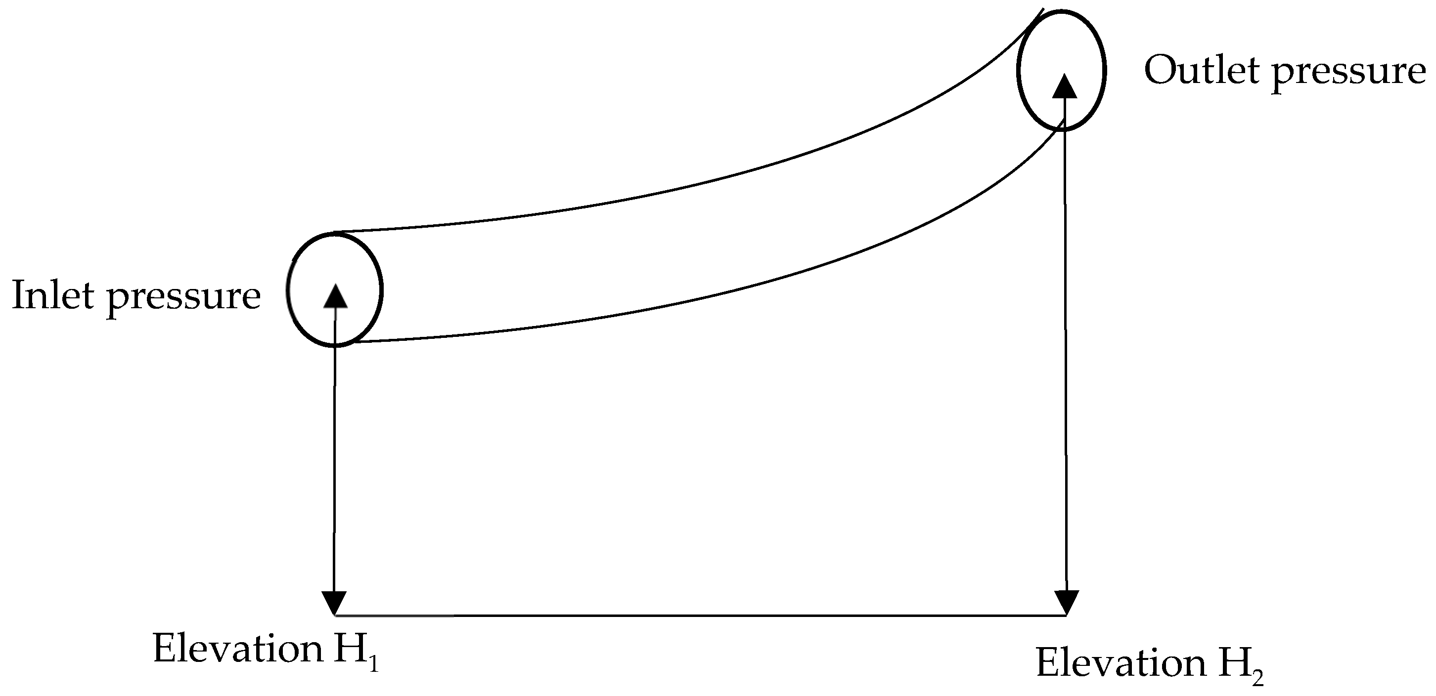
Considering the elevation parameter, there can be two cases: (i) a pipeline without an elevation difference, as shown in Figure 4, (ii) a pipeline with an elevation difference—that is, a height difference between two segments of a pipeline—as shown in Figure 5. The inclusion of an elevation difference along the pipeline introduces an additional parameter, referred to as the elevation adjustment parameter, which is dimensionless and given by Equation (8).

$$s=0.0684 G\left({\displaystyle \frac{H_2-H_1}{T_{f}Z}}\right)$$

(8)

H₁ and H₂—Inlet and outlet elevations (m).

s—Elevation adjustment parameter (dimensionless).

Z—Compressibility factor (dimensionless)

T_f—Gas flow temperature in (K)

Considering the effect of elevation, the length of the pipeline is now addressed as an equivalent length, which is represented by Equation (9):

$$L_e=L\left({\displaystyle \frac{e^s-1}{s}}\right)$$

(9)

With this, L in Equation (1) is replaced with L_e, the equivalent pipe length in km.

$$Q=0.018\ast \left({\displaystyle \frac{Ts}{Ps}}\right)\ast E\ast 4\ast {\mathit{log}}_{10}\left({\displaystyle \frac{3.7\ast d}{\epsilon }}\right) \ast {\left({\displaystyle \frac{P_1^2-P_2^2}{\gamma \ast L_e\ast Tavg\ast Z}}\right)}^{0.5}\ast d^{2.5}$$

(10)

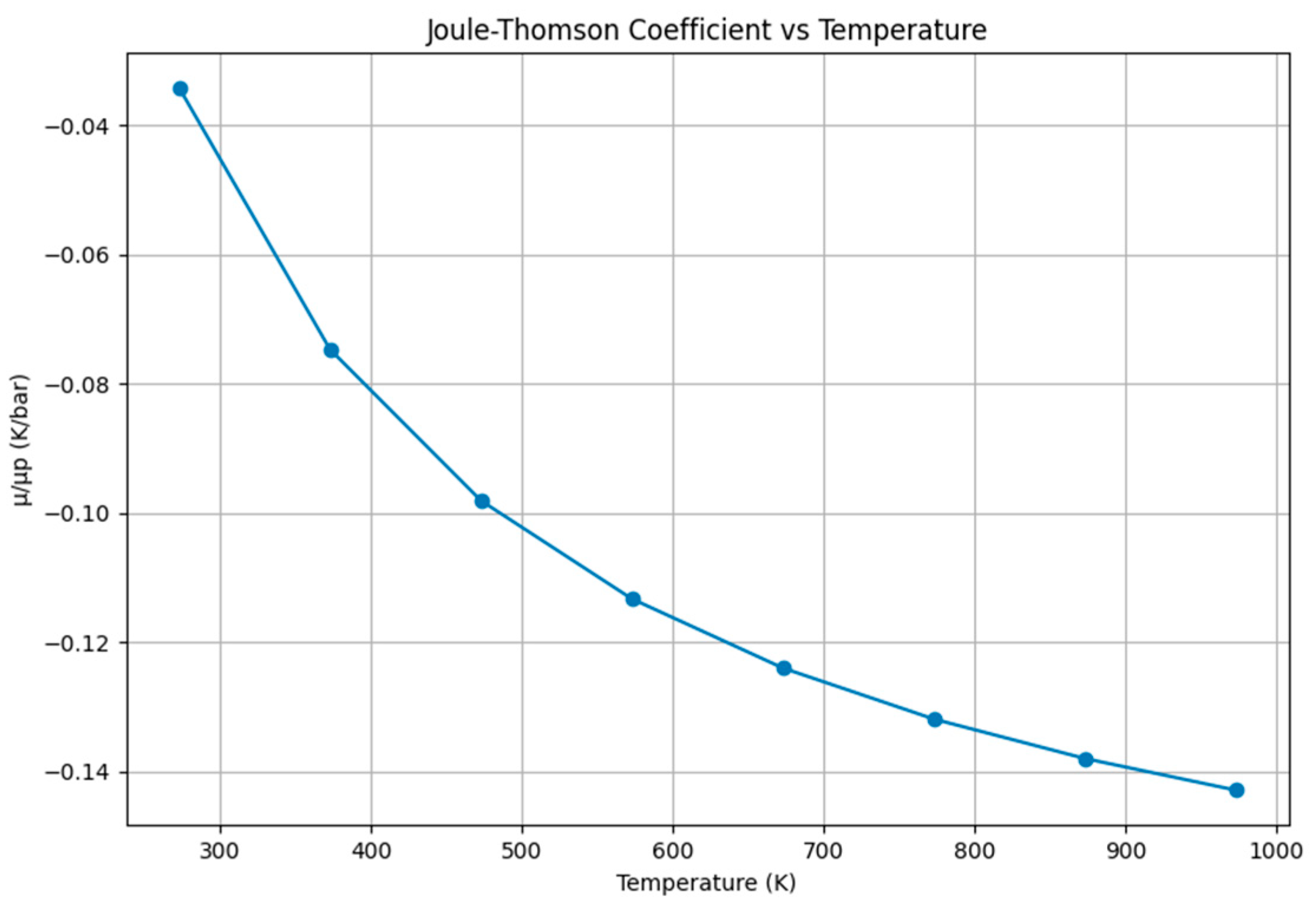
A study on the influence of temperature was performed. All real gases have a specific temperature known as the inversion temperature, where the Joule–Thomson coefficient changes its sign. At ordinary room temperature, the Joule–Thomson coefficient for most gases is positive, except for hydrogen, neon, and helium, and it is 0.5 °K/bar for natural gas and −0.035 °K/bar for hydrogen [11,12]. To establish the temperature effect, Equation (11) is used to determine the temperature values, and it is observed that there was no high spike increase in temperature.

Hydrogen behaves differently and has a Joule–Thomson coefficient (μ_JT) at 1 bar and 300 K of around −0.03 K/bar. The negative sign indicates that, under these conditions, the hydrogen was heated during expansion. The Joule–Thomson coefficient for different gas temperatures of hydrogen is shown in Figure 6. However, the low absolute value of the Joule–Thomson coefficient means that, in practice, the temperature increase of hydrogen will be quite small, except in the case of large pressure changes in a hydrogen refueling station.

The final temperature was calculated using Equation (11).

$$T_2=T_1+{\mu }_{JT} (P_2-P_1)$$

(11)

T₂—Final temperature (K)

T₁—Initial temperature (K)

P₁ and P₂—Initial and final pressure (bar)

${\mu }_{JT}$—Joule–Thomson coefficient (K/bar)

4. CFD Simulation Setup

Computational Fluid Dynamics (CFD) software ANSYS Fluent 2022R1 version was used to perform the simulation in order to analyze the mathematical model and CFD. Due to computational limitations in ANSYS, direct simulation of a 100 km pipeline with a 1 m diameter was not feasible; therefore, the geometry of the model was scaled to 100 m in length and 0.1 m in diameter as an initial stage to analyze and understand the pressure loss phenomenon in a system [13,14], adopting the same surface roughness conditions. In addition to this, the following parameters were considered: (i) material API X52 and its properties [13], (ii) hydrogen gas properties, (iii) preventing reverse flow during simulation, and (iv) material surface roughness 0.00002 m.

As the flow was turbulent in the system, the k-ε turbulent model [15] was selected for the simulation of hydrogen gas in the X52 steel pipe material. The reason for using this model is its importance and robustness, which make it a stable and reliable starting point for CFD analysis. While the AGA Equation focuses on pressure loss due to material surface roughness and friction factor, the k-ε RANS model focuses on the work done by the fluid and solving the Navier–Stokes Equation. The implementation of surface roughness in ANSYS Fluent was performed using wall functions with an equivalent roughness height to represent the overall effect on shear stress and turbulence. Roughness modifies the wall boundary condition through the roughness height (k_s) in the wall function, thereby increasing the shear stress that affects the amount of pressure loss. This is explained with the equation of state.

$$u_{\tau }=\sqrt{{\displaystyle \frac{{\tau }_{\omega }}{{\rho }_{\omega }}} }$$

(12)

$u_{\tau }$—Friction velocity

${\tau }_{\omega }$—Wall shear stress

$${\tau }_{\omega }={\displaystyle \frac{f\rho U^2}{8}}$$

(13)

$f$—Friction factor

U—Mean gas flow velocity

$$u_{\tau }=U\sqrt{{\displaystyle \frac{f}{8}}}$$

(14)

$$k_s^{+}={\displaystyle \frac{k_s{u}_{\tau }}{v_{\omega }}}$$

(15)

$k_s^{+}$ represents dimensionless roughness height. With an increase in the roughness height k_s, $k_s^{+}$ increases, which results an increase in pressure loss.

4.1. Meshing

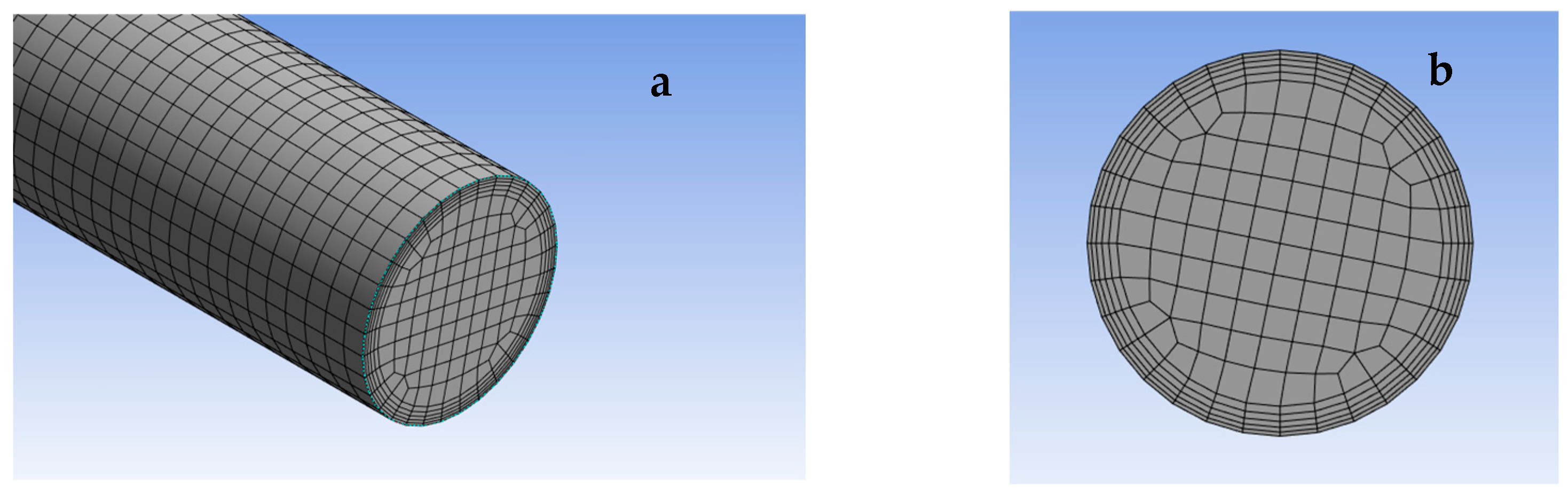
Figure 7a represents the mesh used, and a generated total of 2,396,841 elements were created with a mesh element size of 0.005 m to build the geometry. In addition, an inflation layer was applied to refine the near-wall regions of the mesh. A total of 5 layers were added, as shown in Figure 7b. A grid independence analysis was performed for the assessment of the influence of mesh densities on the accuracy of the results produced by the CFD-based models. The models were developed with different mesh densities. The initial solutions for the simulations were found to have converged. The accuracy of the models was also ascertained by comparing the results produced by the models developed with the 0.002 m and 0.005 m mesh densities. The pressure loss results were found to have been consistent with a maximum deviation of 2.3%. The models developed with the coarse mesh densities of 0.010 m and 0.015 m produced significantly different pressure loss values compared with the results produced by the models developed with the finer mesh densities.

Mesh densities higher than 0.002 m and 0.005 m were found not to have any significant influence, and they also increased the computation times. The models developed with mesh densities of 0.002 m and 0.005 m were found to be appropriate for the purpose. The grid independence study was performed for a representative operating pressure (50 bar), as shown in

Table 1. Effect of element size on pressure loss at 50 bar.

Serial Number	Element Size (m)	Number of Elements	Initial Pressure (bar)	Pressure Loss (bar)
1	0.002	2,514,561	50	0.042
2	0.005	2,396,841	50	0.043
3	0.010	1,258,976	50	0.098
4	0.015	956,731	50	0.125

. Similar trends were observed for pressures in the range of 50–120 bar, confirming the mesh is adequate for all simulations.

An internal inspection using mesh visualization was performed on the model in order to inspect the quality of the mesh generated. Simulations were carried out with an increasing level of refinement in the mesh generated while monitoring and comparing various important parameters in the solutions obtained. The residuals were set at 10⁻⁶ units. It was noticed that an increased level of refinement in the mesh resulted in changes that may be deemed insignificant in the monitored solutions obtained. The discrepancy in the solutions obtained from the medium and fine meshes fell within an acceptable level of tolerance.

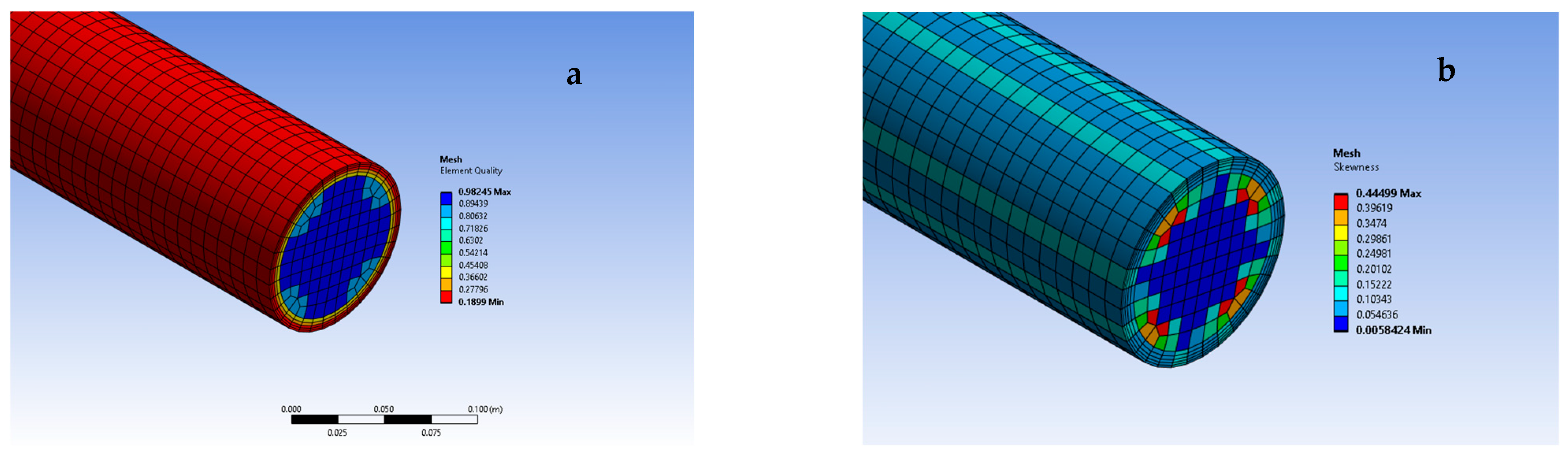
Internal mesh quality inspection was performed as depicted in Figure 8a,b. The aim of this inspection was to verify the mesh quality by checking the mesh quality parameters. The parameters included mesh skewness, aspect ratios, and smoothness. From the mesh inspection, it can be concluded that the mesh configuration adopted was refined enough for the desired results.

4.2. Boundary Conditions

The boundary conditions for the simulation setup were based on a pressure-based solver type. In the Materials section of Fluent, API X52 material properties and fluid hydrogen gas properties were given. The model was split into 3 parts (i) inlet, (ii) wall and (iii) outlet. To begin, the simulation mass flow input type was selected at the input for the wall region no slip condition, and the stationary wall motion type was selected. The roughness height was declared in the wall region, and the standard roughness model was selected. Pressure-outlet type was selected to estimate the pressure at the outlet. To begin the simulation, the initialization was made from the inlet region of the pipe.

4.3. Solution Convergence

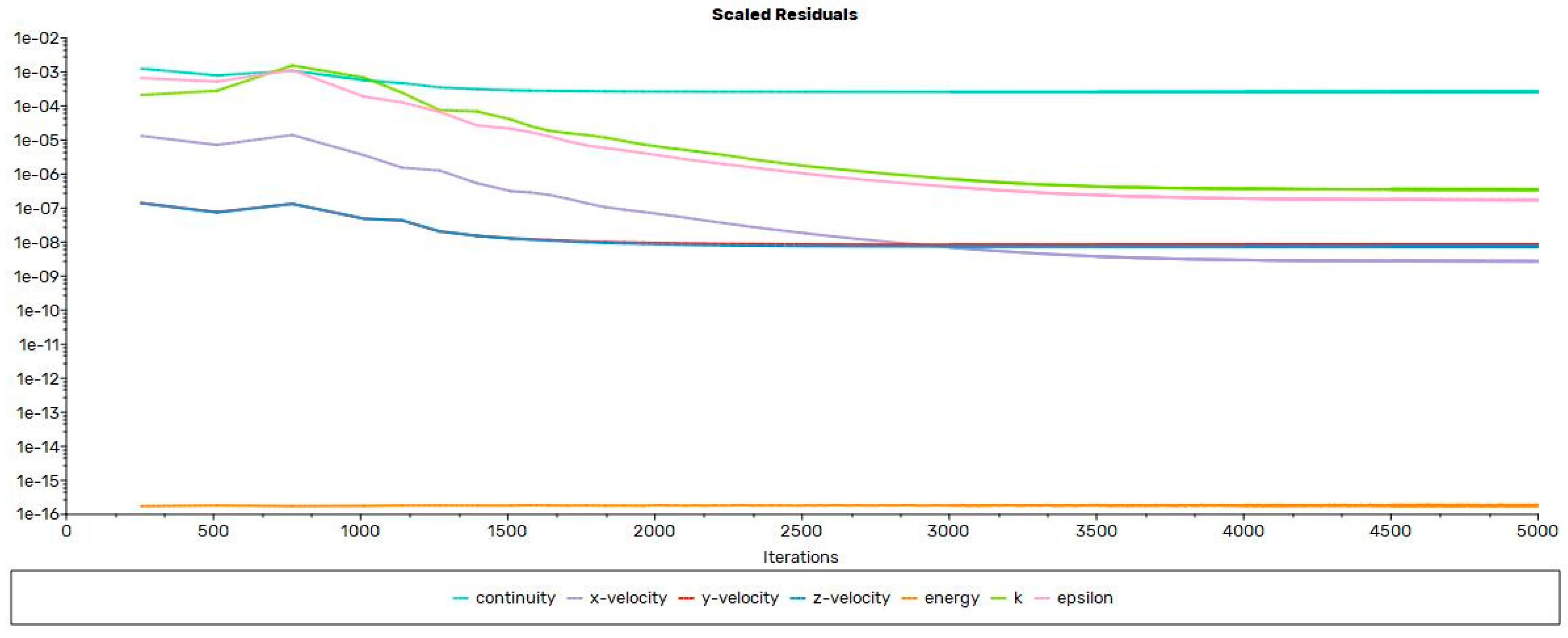
Figure 9 is an illustration of the convergence history of residuals for continuity, momentum, energy, and turbulence variables. All basic equations show a steadily decreasing trend, ensuring numerical stability of the computed solution. The residuals for both momentum and energy show a reduction of more than six orders of magnitude, while energy residuals are reduced to a level of 10⁻¹⁶, ensuring the convergence. The residuals for turbulence show a clean convergence without any oscillations, ensuring proper capture. The residuals for continuity being stabilized at 10⁻⁴ are quite reasonable for high Reynolds number turbulent calculations and are consistent with mass balance. Overall, the residual behavior confirms that the solution is fully converged and numerically reliable.

5. Results

The pressure loss for the full-scale 100 km pipeline was initially calculated using the AGA analytical model. Due to limitations of computational performance in CFD, the pipeline geometry was subsequently scaled down to a length of 100 m and a diameter of 0.1 m. For the scaled model, pressure losses were evaluated using both AGA formulation and CFD simulations, which enable comparison between analytical and CFD under identical operating conditions. The agreement obtained from this comparison was employed to estimate pressure loss for a 100 km pipeline.

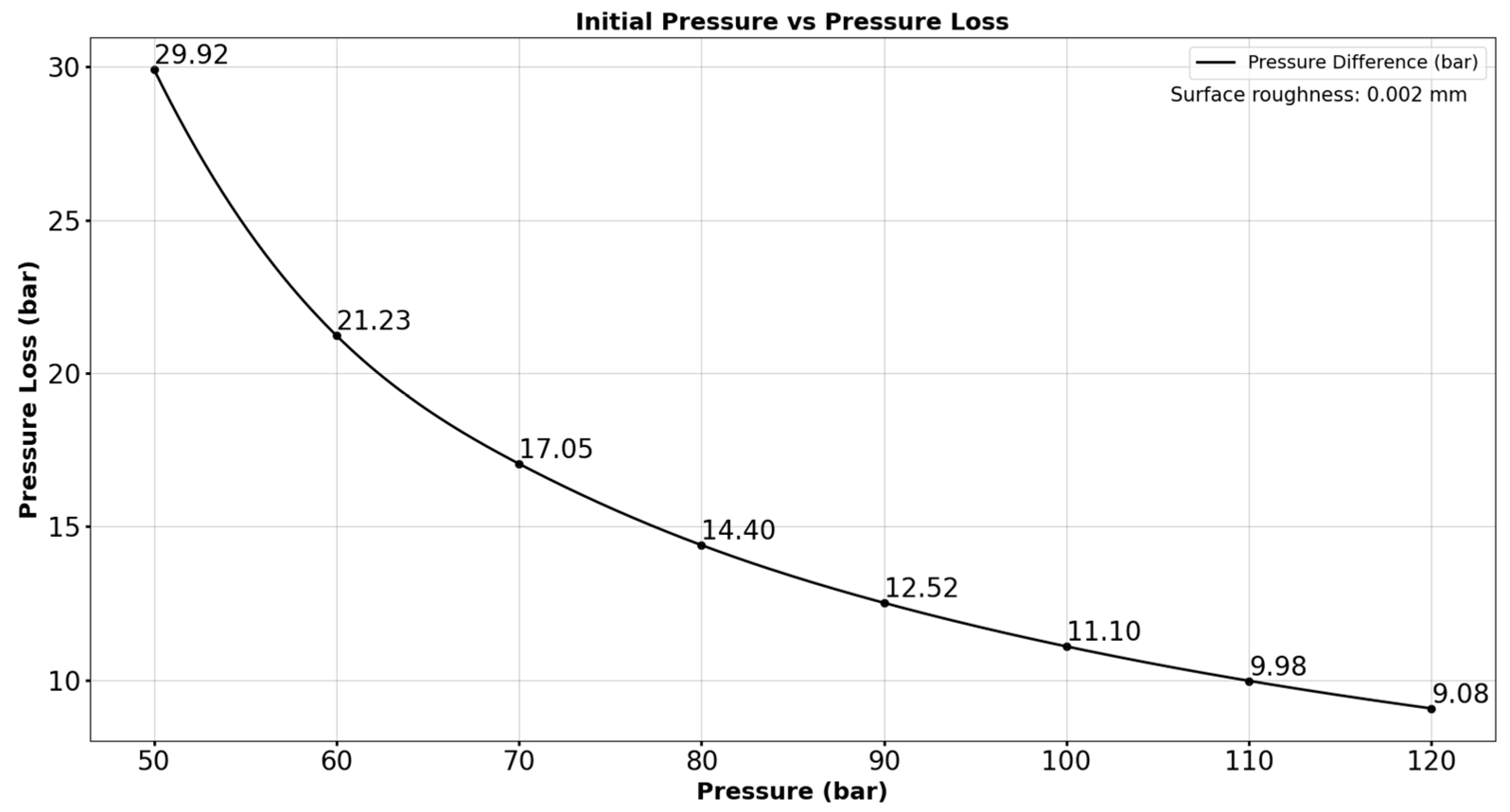
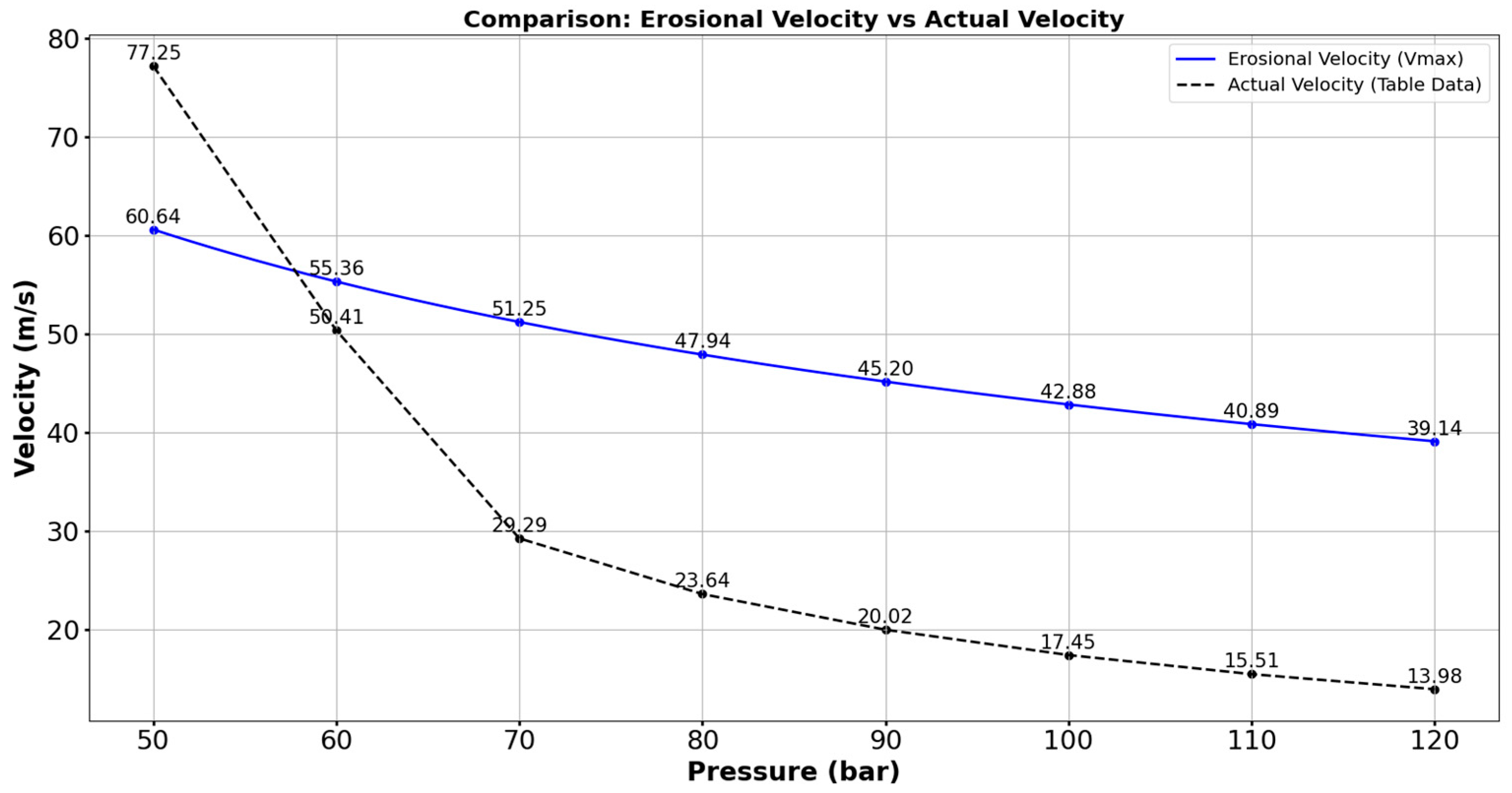
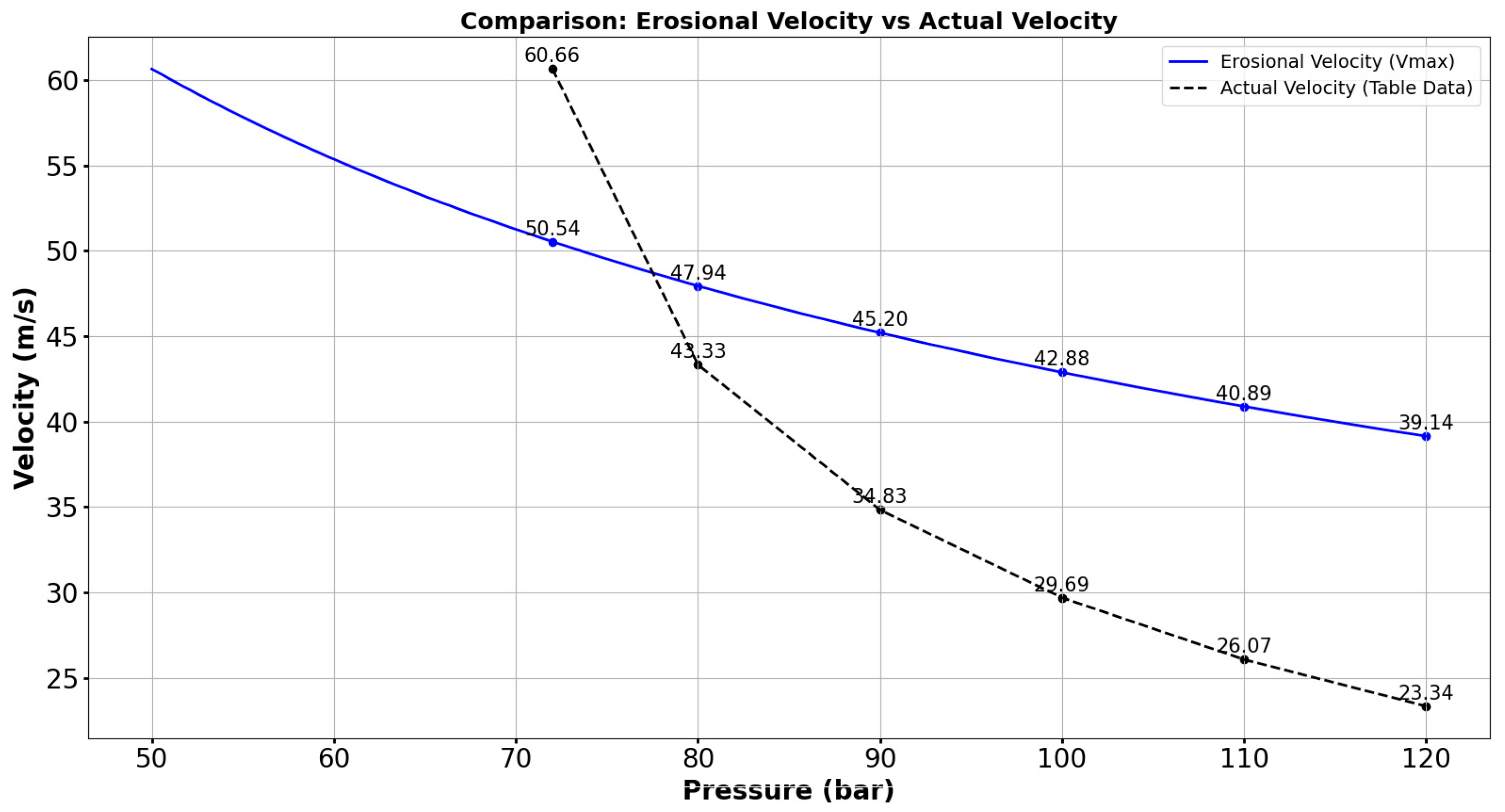
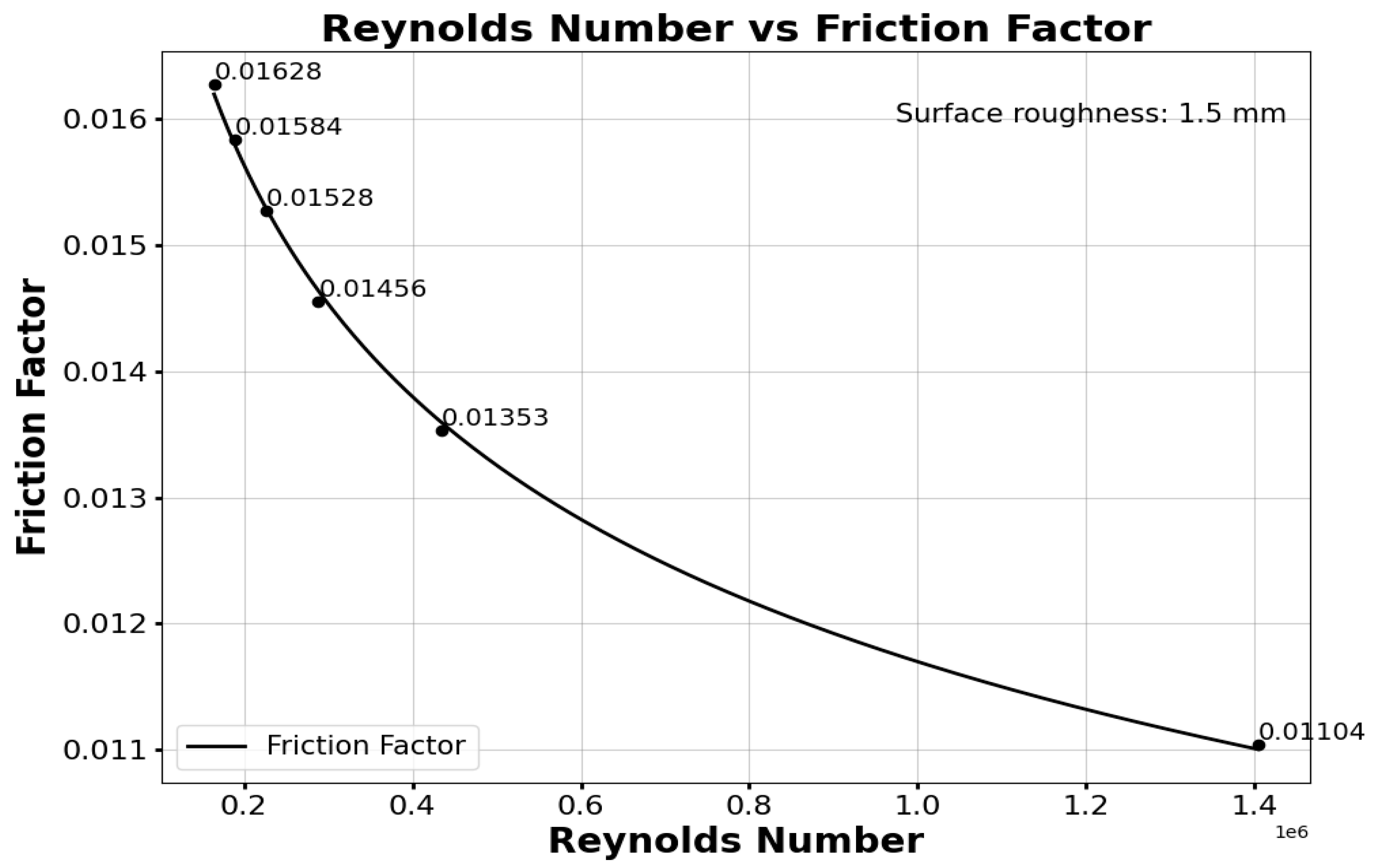
Using the AGA Equation, numerical computation was performed using the Python version 3.11 and Pycharm Community Edition 2024.1.4 software. The results were observed for a distance of 100 km.

Table 2. Pressure loss for 100 km with material roughness of 0.00002 m using AGA.

Initial Pressure in bar	Final Pressure in bar	Pressure Difference in bar	Velocity m/s	Reynolds Number	Friction Factor
50.00	20.08	29.92	77.25	792,606.00	0.014896
60.00	30.77	21.23	50.41	517,220.00	0.015377
70.00	52.95	17.05	29.29	300,523.00	0.016257
80.00	65.60	14.40	23.64	242,552.00	0.016668
90.00	77.48	12.52	20.02	205,410.00	0.017022
100.00	88.90	11.10	17.45	179,041.00	0.017349
110.00	100.02	9.98	15.51	159,136.00	0.017639
120.00	110.92	9.08	13.98	143,438.00	0.017946

shows the pressure loss computed for an initial pressure of 50 to 120 bar, and a graphical representation is shown in Figure 10. The corresponding gas velocity in comparison with the actual velocity for a surface roughness of 0.00002 m is shown in Figure 11. The relation between the friction factor and Reynolds number for 0.00002 m is shown in Figure 12. As the roughness of the material increases, the initial pressure should be increased. The reason to increase the initial pressure is that the pipeline system is not in a condition to accept the pressure values that are used when the pipeline is in good condition with low roughness.

Table 3. Pressure loss for 100 km when the material roughness is 0.0015 m using AGA.

Initial Pressure in bar	Final Pressure in bar	Pressure Difference in bar	Velocity m/s	Reynolds Number	Friction Factor
72.00	11.34	60.66	136.80	1,403,605.00	0.011043
80.00	36.67	43.33	42.30	434,009.00	0.013534
90.00	55.17	34.83	28.11	288,416.00	0.014555
100.00	70.31	29.69	22.06	226,341.00	0.015277
110.00	83.93	26.07	18.48	189,609.00	0.015836
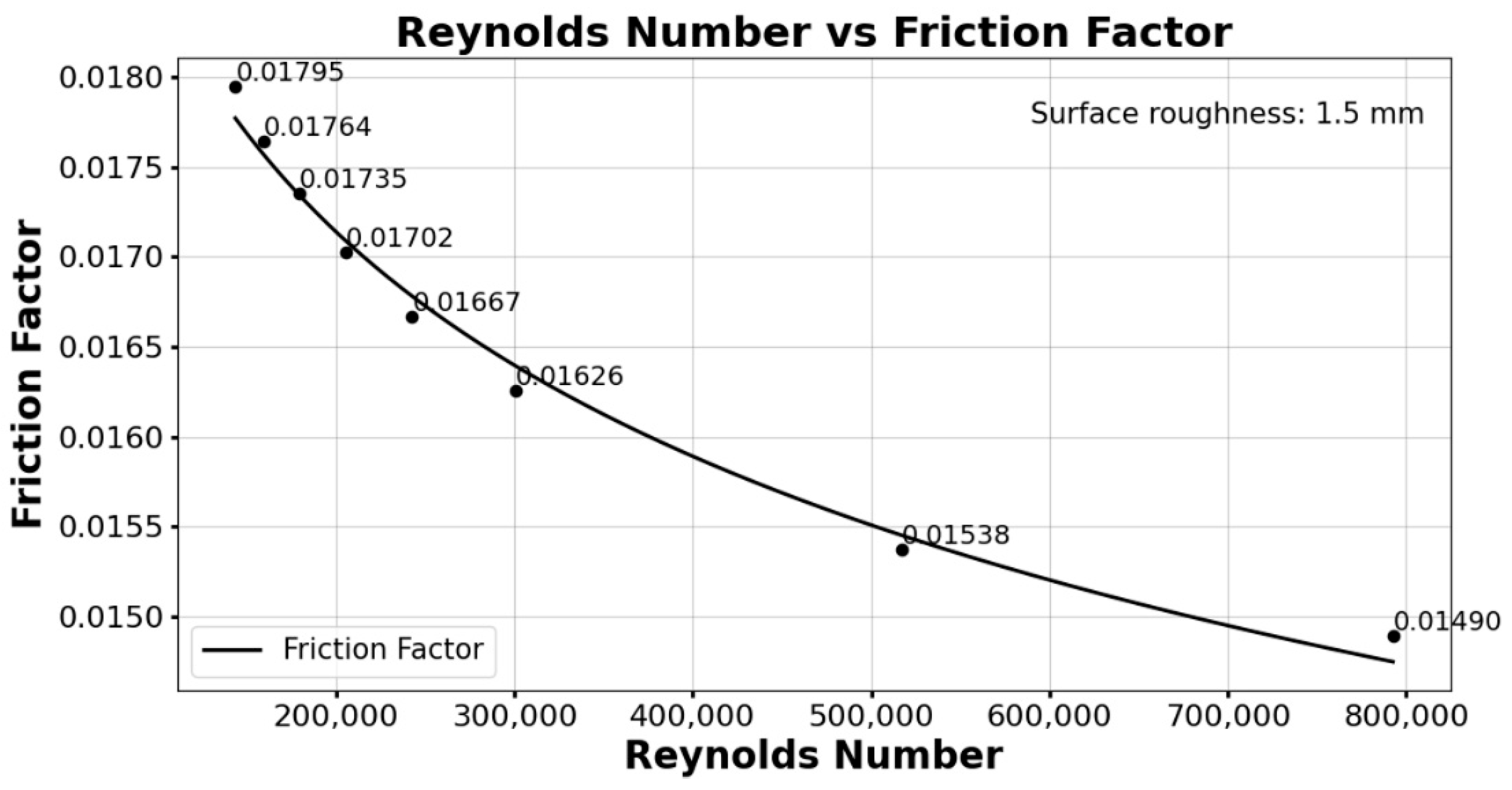
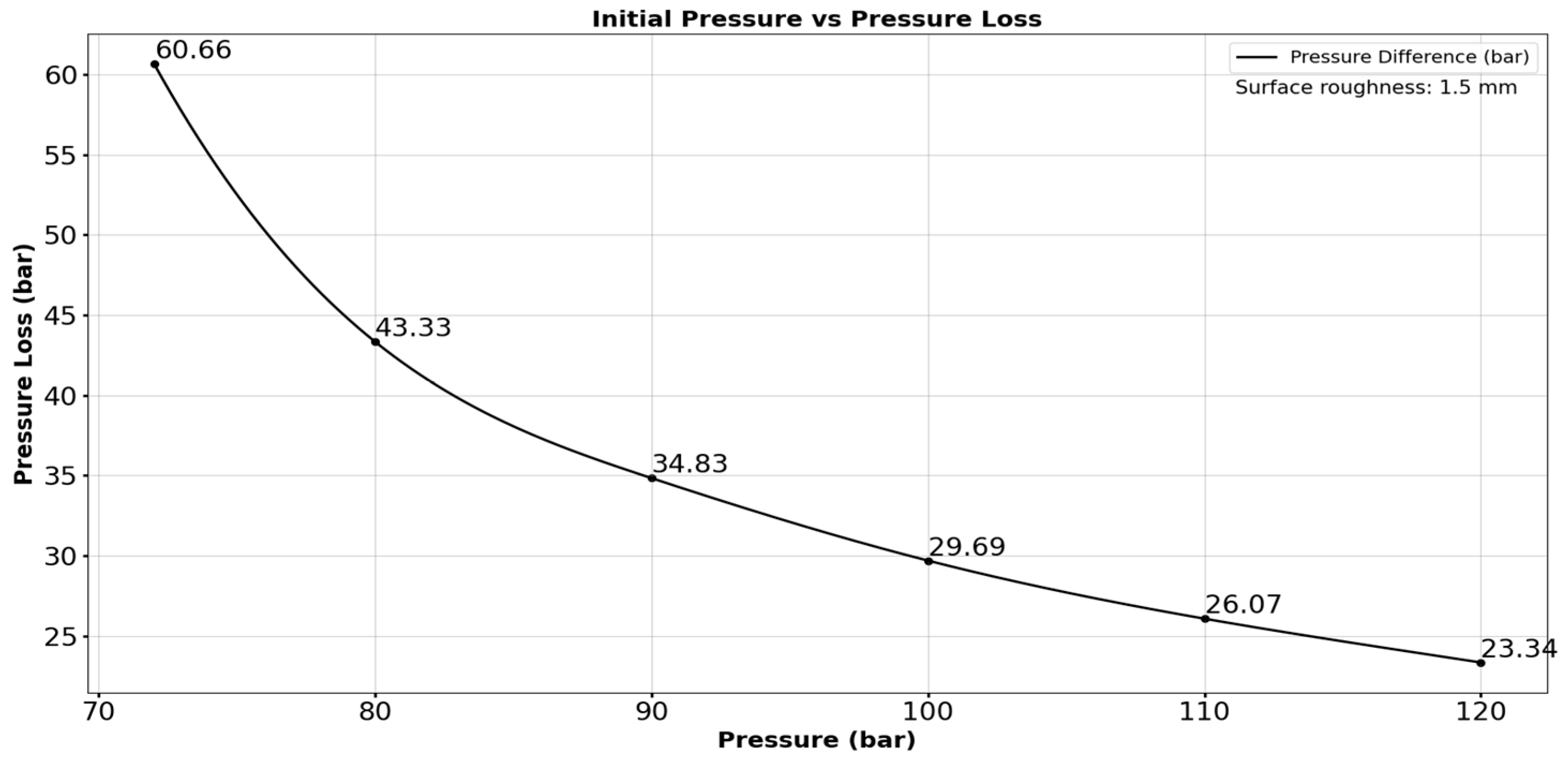
120.00	96.66	23.34	16.04	164,574.00	0.016275

shows the pressure loss when the surface roughness is 0.0015 m. The pressure loss when the roughness is 0.0015 m is shown in Figure 13. The corresponding gas velocity in comparison with the actual velocity for surface roughness 0.0015 m is shown in Figure 14. The relation between the friction factor and Reynolds number for 0.0015 m is shown in Figure 15.

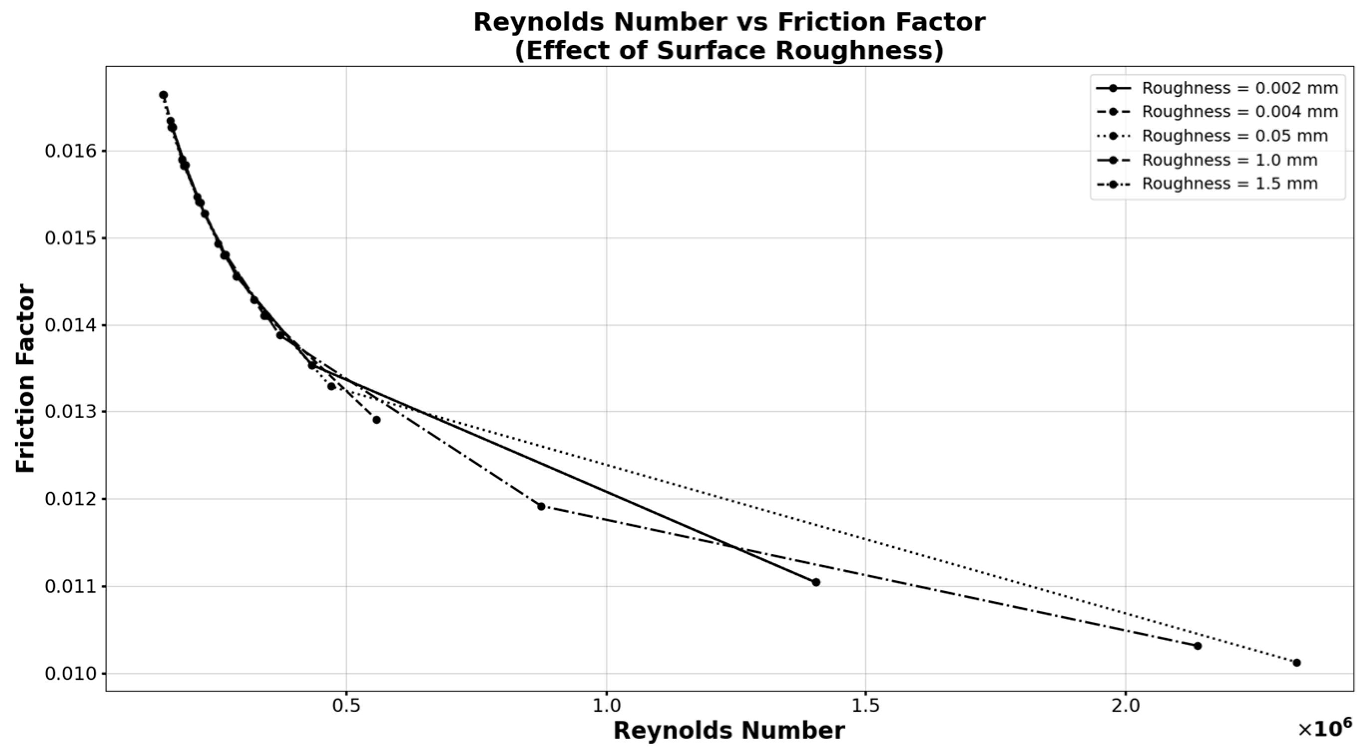
In this study, it was determined that there is an inverse proportion between friction factors and Reynolds numbers, in which friction factors were found to be higher with lower Reynolds numbers, while friction factors were lower with increasing Reynolds numbers. The physical aspects can be explained by considering that, with lower Reynolds numbers, viscous effects exist, which cause wall shear stress to increase, thereby increasing friction factors. The effects of surface roughness on friction factors and Reynolds numbers with different values of roughness are shown in Figure 16.

Table 4. Change in temperature of H₂ gas for surface roughness of 0.00002 m.

Initial Pressure in bar	Final Pressure in bar	Initial Temperature in K	Final Temperature in K	Percentage of Temperature Difference in%
50	20.08	300	301.05	0.35
60	30.77	300	301.02	0.34
70	52.95	300	300.60	0.19
80	65.60	300	300.50	0.16
90	77.48	300	300.44	0.14
100	88.90	300	300.39	0.12
110	100.02	300	300.35	0.11
120	110.92	300	300.32	0.10

shows the variation of hydrogen gas temperature for surface roughness of 0.00002 m, where there is an increase in outlet temperature, though the percentage increase remains less than 0.35%.

Table 5. Change in temperature of H₂ gas for surface roughness of 0.0015 m.

Initial Pressure in bar	Final Pressure in bar	Initial Temperature in K	Final Temperature in K	Percentage of Temperature Difference in%
72.00	11.34	300	302.12	0.70
80.00	36.67	300	301.52	0.50
90.00	55.17	300	301.22	0.40
100.00	70.31	300	301.04	0.34
110.00	83.93	300	300.91	0.30
120.00	96.66	300	300.82	0.27

shows the results for increased roughness of 0.0015 m, where there is an increase in outlet temperature, with the maximum increase being 0.70%.

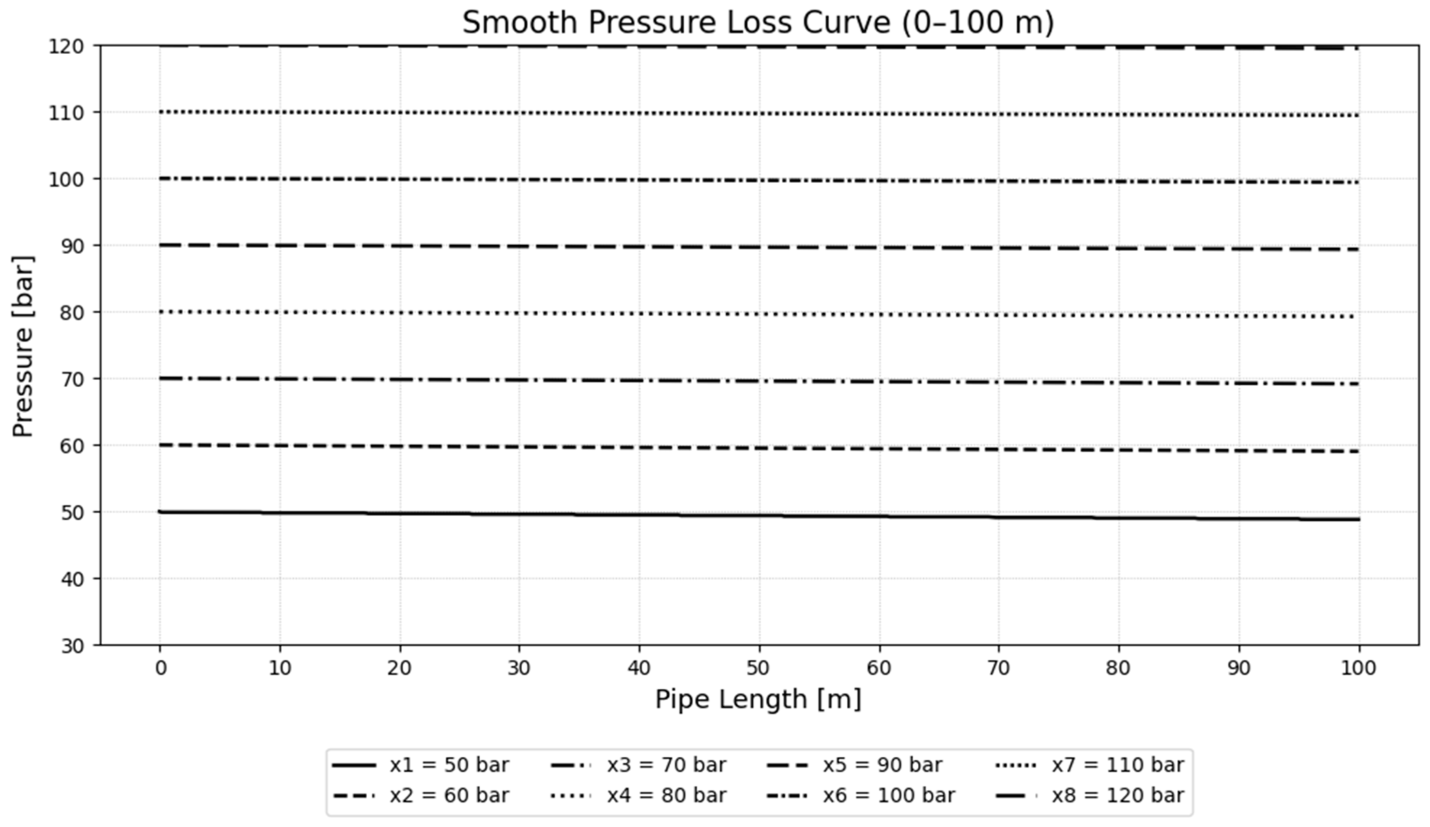
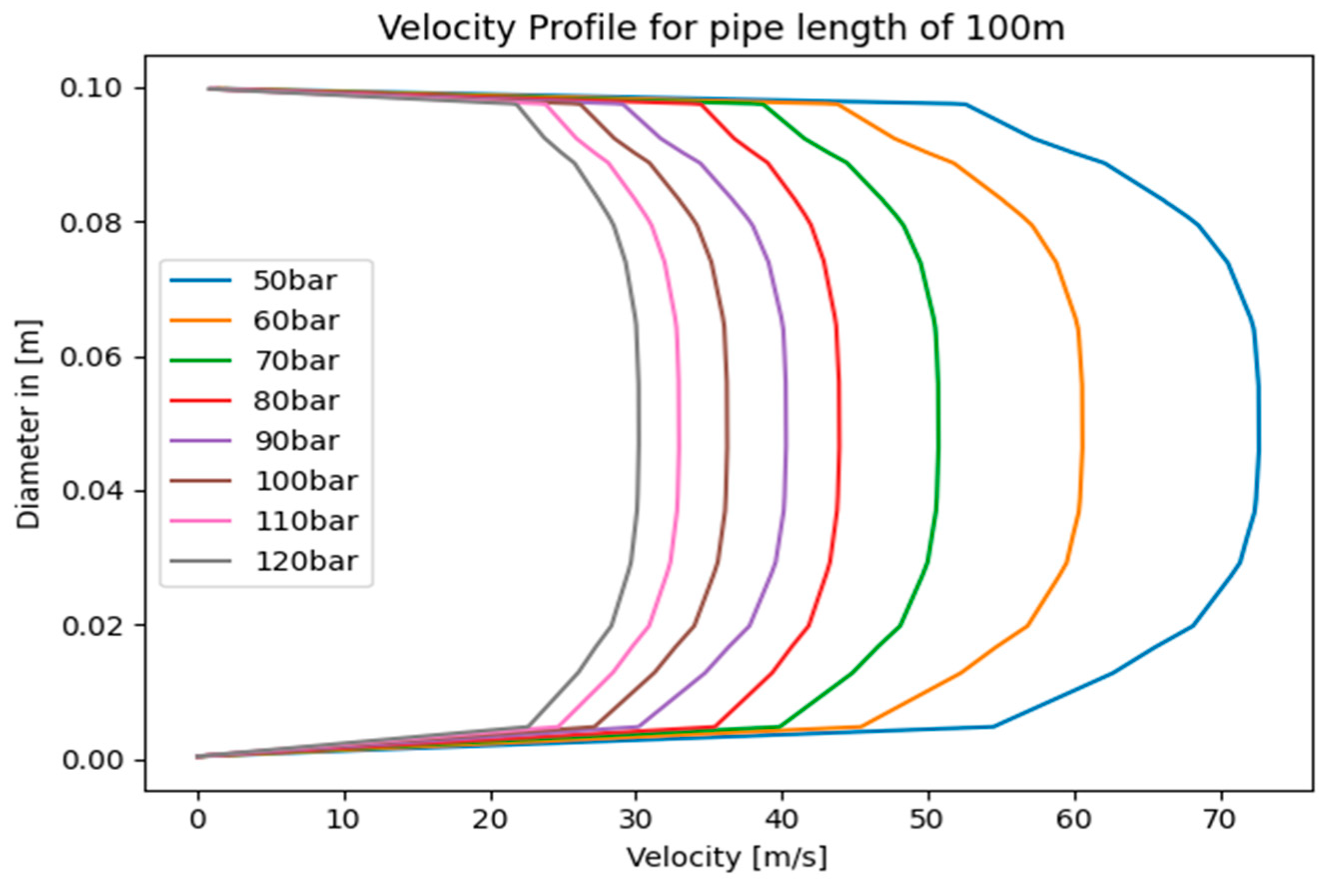
The CFD k-ε model was selected to establish a comparison between CFD and the AGA model for a surface roughness of 0.00002 m. The comparison was made based on the dP/dx area weight average, which was used for the inlet and outlet region of CFD to compute pressure losses over a length of 100 m, as shown in Figure 17. The velocity profile of gas is shown in Figure 18. The AGA and CFD results were computed for 100 m, and a close comparison of pressure loss and velocity of gas was made, as shown in

Table 6. Comparison between AGA and CFD results for 100 m pipe length (roughness = 0.00002 m).

Initial Pressure in bar	Velocity of H2 Gas in m/s		Pressure Loss in bar
	AGA	CFD	AGA	CFD
50	73.78	63.39	0.043	0.053
60	61.20	52.96	0.039	0.045
70	52.40	45.43	0.036	0.039
80	45.95	39.75	0.031	0.036
90	40.68	35.36	0.029	0.032
100	36.59	31.84	0.025	0.029
110	33.25	28.95	0.022	0.025
120	30.46	26.55	0.015	0.021

. The results were used to estimate pressure losses for 100 km, as shown in

Table 7. Comparison between AGA and CFD results for 100 km pipe length (roughness = 0.00002 m).

Initial Pressure in bar	Velocity of H2 Gas in m/s		Pressure Loss in bar
	AGA	CFD	AGA	CFD
50	73.78	63.39	43.39	53.16
60	61.20	52.96	39.45	45.14
70	52.40	45.43	36.63	39.78
80	45.95	39.75	31.21	36.63
90	40.68	35.36	30.23	32.59
100	36.59	31.84	25.11	29.81
110	33.25	28.95	22.01	25.33
120	30.46	26.55	15.23	21.58

.

5.1. Mathematical Validation

The mathematical justification for extrapolating between 100 m and 100 km relies on the Darcy–Weisbach Equation (16).

$${\displaystyle \frac{∆P}{L}}=f· {\displaystyle \frac{\rho V^2}{2 D}}$$

(16)

∆P/L—Pressure loss drop per unit length (pressure gradient)

f—Friction factor

ρ—Density of hydrogen gas

V—Velocity of gas flow

D—Internal diameter of pipe

The friction factor is determined by the Reynolds number, relative roughness, and velocity. Since the gas velocity, inlet pressure, and viscosity are identical, the Reynolds number is preserved. The roughness of 0.00002 m is taken for both the 100 m pipe and the 100 km pipe, with the diameter of pipe held constant. The ratio of roughness to diameter (ε/D) is preserved.

5.2. Validation of the Extrapolation Method

The extrapolation from the model scaled from 100 m to 100 km is seen to be valid because the system maintains dynamic and geometric similarity. The flow physics are governed by the Reynolds number (Re) and relative roughness (ε/D). At equal inlet pressure and velocity, the viscous forces are identical. With constant pipe geometry and material roughness, the geometric similarity is preserved. Since the dimensionless parameters are preserved, the friction factor remains the same. Consequently, the pressure gradient (dP/dx) applied to the 100 m model applies to the 100 km model.

Comparing the results,

Table 8. Validation of scaling model from AGA results.

Initial Pressure (bar)	∆P at 100 m (bar)	∆P at 100 km (bar)	Scaling Factor $\frac{{∆\mathit{P}}_{100\mathbf{k}\mathbf{m}}}{{∆\mathit{P}}_{100\mathbf{m}}}$	Deviation from Linear (%)
50	0.043	43.39	1009	0.91
60	0.039	39.45	1012	1.15
70	0.036	36.63	1018	1.75
80	0.031	31.21	1007	0.68
90	0.029	30.23	1042	4.24
100	0.025	25.11	1004	0.44
110	0.022	22.01	1000	0.05
120	0.015	15.23	1015	1.53

and

Table 9. Validation of scaling model from CFD results.

Initial Pressure (bar)	∆P at 100 m (bar)	∆P at 100 km (bar)	Scaling Factor $\frac{{∆\mathit{P}}_{100\mathbf{k}\mathbf{m}}}{{∆\mathit{P}}_{100\mathbf{m}}}$	Deviation from Linear (%)
50	0.053	53.16	1003	0.30
60	0.045	45.14	1003	0.31
70	0.039	39.78	1020	2.00
80	0.036	36.63	1018	1.75
90	0.032	32.59	1018	1.84
100	0.029	29.81	1028	2.79
110	0.025	25.33	1013	1.32
120	0.021	21.58	1028	2.76

confirm that the length ratio is scaled to 1000:1 (100 km/100 m). The resulting pressure loss ratio is consistently close to this value but exhibits a slight deviation due to compressibility effects. Over the longer pipe length, the gas density decreases more significantly than for the shorter pipe, leading to higher velocities and increasing frictional losses per meter near the outlet. The extrapolation captures this non-linear compressibility effect, confirming that the method is physically robust.

The inlet Mach number is identical for both cases in

Table 10. Mach number and Reynolds number for hydrogen gas flow.

Initial Pressure (bar)	Velocity (m/s)	Speed of Sound (m/s)	Mach Number (Ma)	Reynolds Number (Re)
50	73.78	1334	0.055	6.11 × 107
60	61.20	1338	0.046	6.04 × 107
70	52.40	1342	0.039	6.00 × 107
80	45.95	1346	0.034	5.98 × 107
90	40.68	1350	0.030	5.92 × 107
100	36.59	1354	0.027	5.88 × 107
110	33.25	1358	0.025	5.85 × 107
120	30.46	1361	0.022	5.81 × 107

. Although the flow remains subsonic, preserving this parameter is essential for modelling gas compressibility effects. The Mach number governs the coupling between pressure, density, and velocity variations associated with gas expansion. Matching the inlet Mach number ensures the thermodynamic mechanism of gas expansion is consistent between the 100 m and 100 km pipes. This guarantees that the density gradient observed in the 100 m pipe model is physically representative of the density profile in the 100 km pipe. The speed of sound values were calculated using the real gas thermodynamic relation in Equation (17). To ensure accuracy at high operating pressures (50–120 bar), the calculation accounts for non-ideal behavior of hydrogen by incorporating the compressibility factor (Z), which ranges from 1.03 to 1.07. This results in speed of sound values slightly higher than the standard value, confirming that compressibility effects were appropriately modeled. The Reynolds number decreases slightly with increasing pressure due to a decrease in velocity and an increase in viscosity of hydrogen with pressure. However, the effect of increased density is not dominant. The flow remains fully turbulent at all operating conditions.

$$c=\sqrt{\gamma .Z.R.T}$$

(17)

C—Speed of sound (m/s)

γ—Ratio of specific heat for hydrogen gas (1.40)

Z—Compressibility factor of hydrogen gas

R—Specific gas constant for hydrogen

T—Gas temperature

6. Conclusions

Determining basic thermodynamics parameters of transported gas as a function of pipeline length is helpful in the calculation of pressure drop. With H₂, the pressure drop is high at low initial pressure values and low at high initial pressure values, which is due to significant different velocities of the gas that is travelling inside the pipeline. As the pipeline ages, the material roughness increases with time, due to which it is observed that the pressure losses are even higher, and it is not possible to start the gas at an initial pressure of 50 bar like when the pipeline is in new condition. The compression station has been excluded in this current analysis to quantify the pressure loss resulting from its absence.

In this study, two extreme cases of pipeline conditions were used: when the pipeline is in new condition, and when the pipeline is severely corroded, impacting the roughness of the material. Further, this work analyzes variations in volumetric flow rate to determine their impact on pressure loss and flow conditions within the pipeline.

The role of pipeline efficiency is seen as important. Pipeline efficiency is representative of pipeline operation conditions with the time of usage. Further computation involves different scenarios to compute and compare the pressure losses with different conditions that mainly involve the phases of pipeline that come in between the new pipeline and severely corroded phase, with metrics including the pipeline efficiency, change in volumetric flow rate, elevation differences, and pipeline distance.

The results presented provide a comparison between mathematical model results and CFD results. The following observations were made.

• The AGA analytical model and CFD simulations both show a decrease in velocity and pressure loss as inlet pressure increases.
• CFD results predict systematically higher-pressure losses than the AGA model. This is due to details of the flow physics captured by CFD during simulation.
• The scaled pipeline analysis demonstrates good qualitative agreement between AGA and CFD results.
• The change in velocity has a significance effect on the Reynolds number and friction factor, which results in pressure losses.
• During the mathematical modelling, it was observed that pressure losses were significantly higher for pipes with smaller diameters, and lower pressure losses were observed for pipes with larger diameters due to the effect of the surface-to-volume ratio of the pipe.
• As the pipe internal surface roughness increases from 0.00002 m to 0.0015 m, the friction factor increases by 2.7 times, resulting in a drastic reduction in pressure difference for the gas flow. This indicates that an initial pressure of 50 bar is sufficient for a smooth pipe with a roughness of 0.00002 m, as shown in Table 1. An additional value of 72 bar is necessitated for pipes with a roughness of 0.0015 m, as shown in Table 2, to obtain an equivalent flow rate because of a lower transmission factor F.
• The extrapolation from the 100 m model to the 100 km prototype is validated by the preservation of dynamic and geometric similarities (Re, Ma and ε/D). The pressure loss results scale consistently with the 1000:1 length ratio while correctly capturing the non-linear deviation due to gas compressibility. This confirmation method is mathematically valid.

The correlations are validated based on comparisons between CFD calculation and analytical calculations based on the AGA method. Experimental validation of the proposed correlation on lab scale pipe will be considered for future studies as a verification of pressure loss measurement. Also, the proposed study is restricted to the pressure loss of straight pipes and does not take into consideration the pressure losses associated with fittings like bends, valves and intersections.

In conclusion, the selection of pipeline material is critical, particularly regarding specific properties such as surface roughness, which has a direct influence on the pressure loss. To overcome this, regular maintenance of pipelines must be performed with the application of a material coating on the internal surface of pipes, which is one of the methods used to maintain the roughness of the material. As the rate of surface roughness increases, the pressure losses in the pipeline also increase. The material surface roughness must be maintained within the limit before it reaches higher values to keep minimal pressure losses in pipelines. Although natural gas pipelines are constructed from carbon steel, their direct application to hydrogen transport is restricted due to hydrogen embrittlement and enhanced permeability. These challenges indicate using low-strength steels such API X52 grade to ensure safe operation of hydrogen pipelines.

References

1. Kuczyński, S.; Łaciak, M.; Olijnyk, A.; Szurlej, A.; Włodek, T. Thermodynamic and Technical Issues of Hydrogen and Methane-Hydrogen Mixtures Pipeline Transmission. Energies 2019, 12, 569. [Google Scholar] [CrossRef]
2. Haeseldonckx, D.; D’haeseleer, W. The Use of The Natural-Gas Pipeline Infrastructure for Hydrogen Transport in A Changing Market Structure. Int. J. Energy 2007, 32, 1381–1386. [Google Scholar] [CrossRef]
3. Khan, M.A.; Young, C.; Layzell, D.B. The Techno-Economics of Hydrogen Pipelines. Transit. Accel. Tech. Briefs 2021, 1, 1–40. [Google Scholar]
4. Jottrand, S.; Hendrick, P. Centrifugal Compressor Preliminary Design Optimization for a Hydrogen Pipeline Compression Station. In Turbo Expo: Power for Land, Sea, and Air; American Society of Mechanical Engineers: New York, NY, USA, 2024. [Google Scholar] [CrossRef]
5. Hydrogen Pipeline Systems Igc Doc 121/14 Revision of Doc 121/04, European Industrial Gases Association AISBL. Available online: https://www.eiga.eu/ct_documents/doc121-pdf/ (accessed on 27 September 2025).
6. Bambore, A.; Hendrick, P.; Philippe Ponthot, J. Study, Modelling and Computing Pressur Losses in GH2 Pipelines. In Proceedings of the 20th Conference on Sustainable Development of Energy, Water, and Environment Systems, Dubrovnik, Croatia, 5–10 October 2025; pp. 1–9. [Google Scholar]
7. American Gas Association (AGA) Equation for Fully Turbulent Isothermal Gas Flow (Reference: Eq-17–18, Section 17, GPSA Engineering Data Book, Eleventh Edition, 1998. Available online: https://www.cheresources.com/Single_Phase_Gas_Pipeline_Flow_preview.pdf (accessed on 12 January 2025).
8. Menon, E.S. Gas Pipeline Hydraulics; CRC Press: Boca Raton, FL, USA, 2025; ISBN 0-8493-2785-7. [Google Scholar]
9. Włodek, T.; Łaciak, M.; Kurowska, K.; Węgrzyn, Ł. Thermodynamic analysis of hydrogen pipeline transportation—Selected aspects. AGH Drill. Oil Gas 2016, 33, 379–395. [Google Scholar] [CrossRef]
10. Abbas, A.J.; Hassani, H.; Burby, M.; John, I.J. An Investigation into the Volumetric Flow Rate Requirement of Hydrogen Transportation in Existing Natural Gas Pipelines and Its Safety Implications. Gases 2021, 1, 156–179. [Google Scholar] [CrossRef]
11. Haeseldonckx, D. Concrete Transition Issues Towards a Fully-Fledged Use of Hydrogen as an Energy Carrier. Ph.D. Thesis, KU Leuven, Leuven, Belgium, August 2009. [Google Scholar]
12. Raj, A.; Larsson, I.S.; Ljung, A.L.; Forslund, T.; Andersson, R.; Sundström, J.; Lundström, T.S. Staffan Lundstrom, Evaluating hydrogen gas transport in pipelines: Current state of numerical and experimental methodologies. Int. J. Hydrogen Energy 2024, 67, 136–149. [Google Scholar] [CrossRef]
13. Kurz, R.; Lubomirsky, M.; Bainier, F. Hydrogen in pipelines impact of hydrogen transport in natural gas pipelines. In Turbo Expo: Power for Land, Sea, and Air; American Society of Mechanical Engineers: New York, NY, USA, 2020. [Google Scholar]
14. Tan, K.; Mahajan, D.; Venkatesh, T.A. Computational Fluid Dynamic Modeling of Methane-Hydrogen Mixture Transportation in Pipelines: Understanding the Effects of Pipe Roughness, Pipe Diameter and Pipe Bends. Int. J. Hydrogen Energy 2024, 49, 1028–1042. [Google Scholar] [CrossRef]
15. Anderson, J.D., Jr.; Wendt, J. Computational Fluid Dynamics; McGraw-hill: New York, NY, USA, 1995; ISBN 0-07-001685-2. [Google Scholar]
Figure 1. Schematic representation of a hydrogen gas pipeline.
Energies 19 00885 g001
Figure 2. Compressibility factor for hydrogen gas for different temperatures.
Energies 19 00885 g002
Figure 3. Erosional velocity limit corresponding to the H2 pressure.
Energies 19 00885 g003
Figure 4. Schematic representation of a GH2 pipeline with no elevation difference.
Energies 19 00885 g004
Figure 5. Schematic representation of a GH2 pipeline with elevation difference.
Energies 19 00885 g005
Figure 6. Joule–Thomson coefficient for hydrogen gas at different temperatures.
Energies 19 00885 g006
Figure 7. (a) Isometric mesh view of pipe 100 m in length and 0.1 m in diameter, (b) Inflation layers in the pipe model of 100 m length and 0.1 m diameter.
Energies 19 00885 g007
Figure 8. (a) Element quality of mesh; (b) Skewness of mesh of pipe 100 m and 0.1 m diameter.
Energies 19 00885 g008
Figure 9. Residuals convergence of the CFD solution.
Energies 19 00885 g009
Figure 10. Pressure loss vs. initial pressure for surface roughness of 0.00002 m.
Energies 19 00885 g010
Figure 11. Erosional velocity and actual velocity for surface roughness of 0.00002 m.
Energies 19 00885 g011
Figure 12. Reynolds number and friction factor for surface roughness of 0.00002 m.
Energies 19 00885 g012
Figure 13. Pressure loss vs. initial pressure for surface roughness of 0.0015 m.
Energies 19 00885 g013
Figure 14. Erosional velocity and actual velocity for surface roughness of 0.0015 m.
Energies 19 00885 g014
Figure 15. Reynolds number and friction factor for surface roughness of 0.0015 m.
Energies 19 00885 g015
Figure 16. Reynolds number and friction factor relation for different surface roughness values.
Energies 19 00885 g016
Figure 17. H2 pressure losses over a distance of 100 m for different gas pressures (roughness = 0.00002 m).
Energies 19 00885 g017
Figure 18. Velocity profile of H2 gas in pipeline for surface roughness of 0.00002 m.
Energies 19 00885 g018