Rotating Electric Machine Fault Diagnosis with Magnetic Flux Measurement Using Deep Learning Models

Abstract

This paper presents new techniques for electric machine diagnostics that combine advanced signal processing and artificial intelligence (AI)-based techniques using magnetic flux measurements acquired under various operating conditions. Developing an effective electric machine diagnostics tool is paramount for increased industrial productivity and extending the service life of the machine. The existing diagnostic tools face issues, including false indication of faults using classical methods, and the proposed data-driven methods based on machine learning lack transferability of model knowledge on an unseen dataset from different motor types or power ratings due to structural differences. To overcome these diagnostic drawbacks of statistical ML classifiers and classical approaches, innovative feature selection methods were employed in this work to preprocess the measured magnetic flux into a spectrogram image, and the transfer learning (TL) technique was applied to fine-tune convolution neural networks (CNNs) ImageNet pretrained models. The experimental results show the trained statistical ML classifiers and traditional CNN performance on unseen BU data and on the external data, and the performance demonstrated a lack of generalization on external datasets of different power ratings or structures. Models with such drawbacks cannot be used for developing effective diagnostic systems. The TL technique was employed on different deep CNN ImageNet pretrained models with spectrogram images as inputs to the deep CN network. This approach demonstrated an advanced and improved electric machine diagnostic system that addresses the drawbacks of the current ML-based diagnostic systems. The generalized model developed using CNN ResNet50 outperformed other deep CNN ImageNet models in correctly diagnosing faults on both the dataset generated from the authors’ lab and on an external dataset of a different machine from another research lab.

1. Introduction

The widespread use of electric machines in homes and industry applications makes the development of a reliable diagnostic model for machines imperative for increased industrial productivity [1]. Among all the machine types or designs, induction motors (IMs) are mostly used because of their low cost, ruggedness, and versatility, but mounting problems, lubrication issues, electrical discharge, overloading, and other issues can shorten their service life [2,3,4,5,6,7,8]. Unplanned failures in motors and generators result in substantial productive downtime, high maintenance costs, and safety hazards that can lead to death. Therefore, condition monitoring for early detection of electric machine anomalies is essential to ensure reliability, efficiency, and safety. Several diagnostic approaches applying vibration analysis have proven effective in detecting some faults such as broken rotor bars, bearing faults, gearbox, misalignment, and unbalanced rotor [3]. However, these vibration analysis approaches are effective only on mechanical faults, including mass unbalance, misalignment, bearing faults, and mechanical losses. A widely used method in the condition monitoring field is motor current signature analysis (MCSA), where the time waveform data of the stator current is transformed into a frequency spectrum to observe the frequency components produced by the fault [4]. Flux measurement analysis is similar to MCSA, except that the flux analysis is more efficient at detecting early-stage faults since it is a direct measurement, unlike MCSA, which is an indirect measurement. However, flux measurement analysis is more effective for electrical faults such as eccentricity, broken rotor bar, and stator winding issues than mechanical faults and is particularly less effective for incipient mechanical faults. During the inception of mechanical faults, the amplitude of the flux signal may increase but that may not be enough to identify the nature of the fault. In Ref. [5], the authors demonstrated the ineffectiveness and shortcomings of flux measurement analysis for both mechanical and electrical faults.

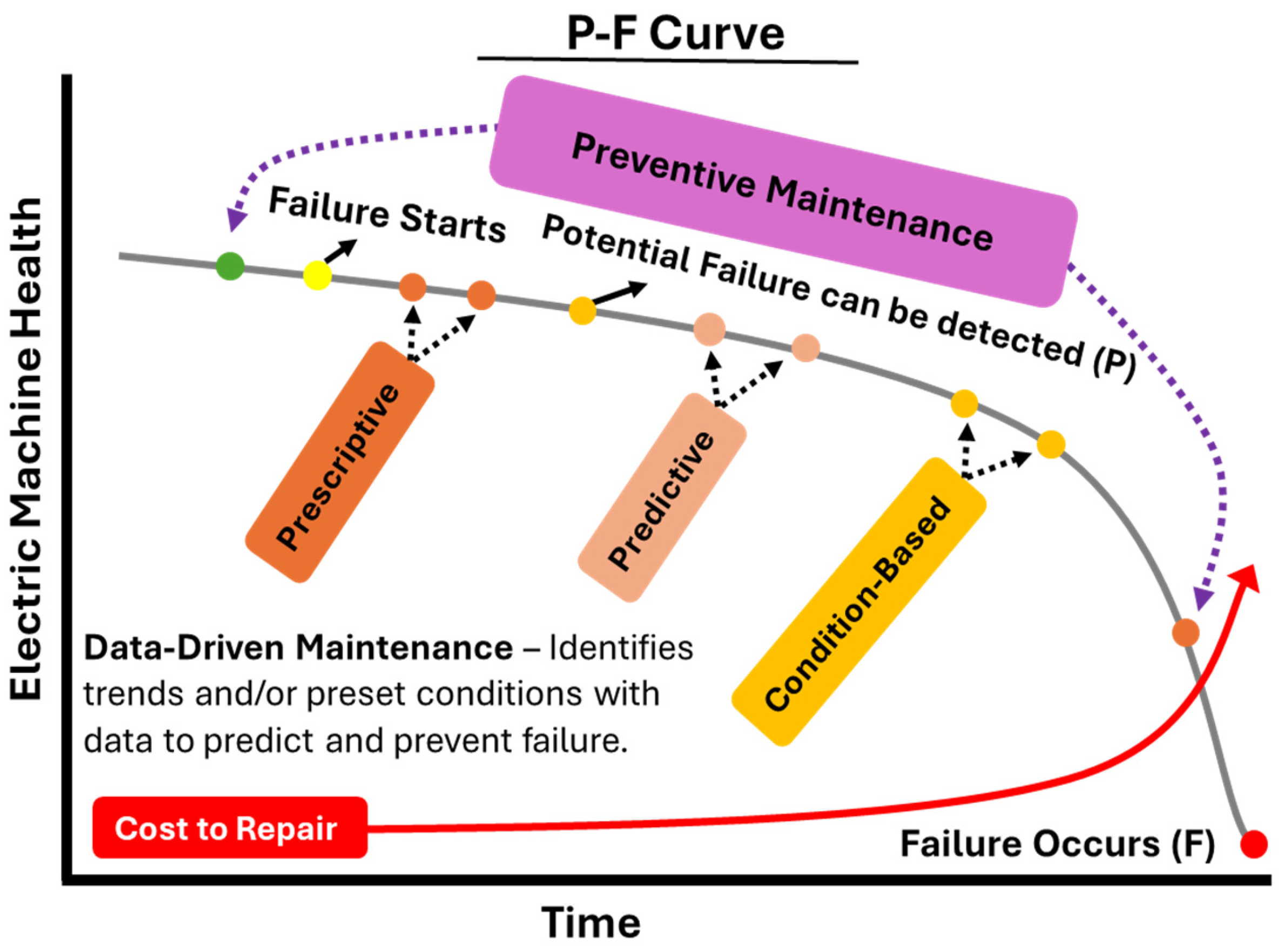
Recent tools for big data processing are becoming valuable tools for solving some of the toughest challenges in electric machine condition monitoring and diagnosis. However, there is still an enormous amount of work needed to integrate these methods into the mainstream operation of industrial facilities. Currently, there are numerous data-driven maintenance techniques and determining which one to use depends on the application, considering reliability and cost, whether to employ simple preventive maintenance or a proactive strategy, as shown in Figure 1. In general, rotating machinery diagnostics can be viewed as the utilization of machinery-measured data in conjunction with technical knowledge to derive meaningful insights about the overall health of the machine, as well as to identify mechanical and electrical faults, their root causes, and potential solutions [9,10,11,12,13].

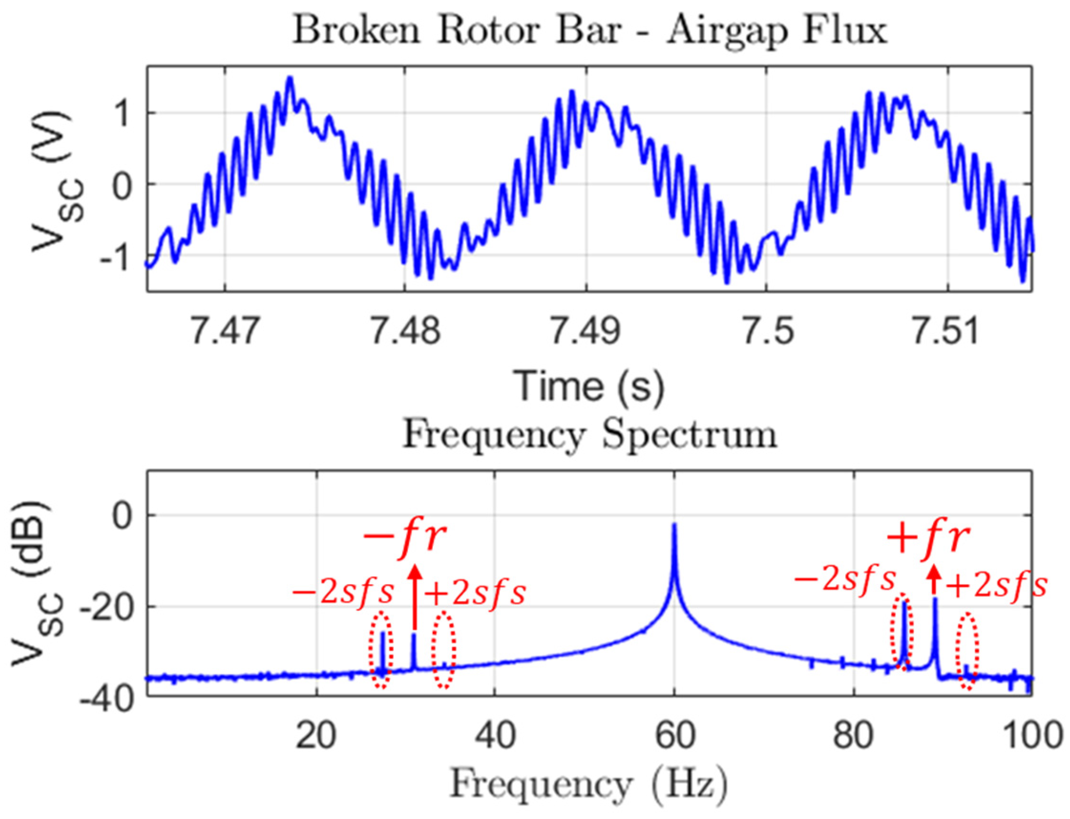
Figure 1 shows the potential failure (P-F) curve for different maintenance strategies and stages, depending on the diagnostic method chosen based on the cost and return on investment. All machinery diagnostics fall under two main categories: conventional and intelligence-based methods. Conventional machine diagnostics can be signal-based or model-based and usually analyzed using classical approaches. These approaches are based on spectral analysis for sidebands to indicate fault conditions. References [1,14,15,16] suggested various methods for detecting static eccentricity (SE) and dynamic eccentricity (DE) using a search coil and stray flux. However, spectral analysis for sidebands requires domain expertise and is prone to issues of false indications, especially early during stages of failure. Figure 2 shows the spectral plot of a broken rotor bar, where domain expertise is required to indicate the fault condition using sidebands. At early failure stages, faulty signatures are often low in amplitude and can be easily masked by electromagnetic noise like harmonics from grid supply or inverter switching effects, mechanical noise such as shaft vibrations or load coupling, and operational variations such as load, speed, or thermal effects. Hence, this results in false negatives (missed faults) or false positives (false alarms), limiting the reliability of signal-based methods [17,18].

Modern approaches combine advanced signal processing, such as power spectral density (PSD), spectrogram analysis, and Empirical Mode Decomposition (EMD), and AI-based techniques with multiple sensor datasets acquired using an advanced data acquisition device that offers high fidelity for real-time monitoring, significantly improved diagnostics, enabling automated fault detection using flux measurement, since airgap flux is a direct indicator of magnetic flux distortion [10,18].

AI- and ML-based techniques typically require large, labeled datasets to achieve high accuracy of fault classification. In practice, fault datasets are scarce, and healthy data is abundant because machines are designed to avoid failure. Also, certain faults, such as broken rotor bar or eccentricity progression, are difficult to replicate experimentally without damaging the equipment. Furthermore, models trained on one machine mostly fail when applied to another machine, due to structural differences, power ratings, or operating conditions. This lack of transferability or generalization severely restricts the industrial adoption of ML-based diagnostic models, since it is impractical to retrain and relabel models for every new machine type.

This paper presents a novel rotating electric machine diagnostics method that integrates advanced signal processing and deep CNN models to outperform the traditional statistical ML algorithms and CNN models. The proposed method focuses on model generalization and industrial implementation of a diagnostic framework using magnetic flux measurement and transfer learning techniques to tackle the challenges of a few faulty datasets in real-world motor diagnostics. Experimental results have been used to compare the performance of statistical ML classifiers, traditional CNN, and the proposed generalized model using deep CNN ResNet50, which can generalize across different machines, regardless of motor type, power rating, or manufacturer, and can be deployed for industrial diagnostics. This can enable industrial real-time on-site diagnostic environments and simultaneous monitoring of multiple machines.

2. Electric Machines Diagnostic Approaches

2.1. Electrical Motor Faults and Electromagnetic Vibration Signatures

The operational performance of machines largely depends on magnetic interaction with mechanical structures. When the magnetic field inside the airgap of the machine is non-uniform, it will produce unbalanced magnetic forces and excite vibrations across the mechanical structures of the machine [19]. Electric machines usually experience three categories of vibrations: mechanical, electromagnetic, and aerodynamic. In most electric machine installations, mechanical vibration can be eliminated at the installation stage by proper alignment, but electromagnetic vibration is likely to occur during operation. Investigating this vibration type can help evaluate the electric machine’s operating performance.

Under healthy conditions, the airgap magnetic field is uniform since the rotor and stator are concentric, and the total force of the radial electromagnetic force is zero. During abnormal conditions, an unbalanced magnetic force (UMF) is produced due to mechanical or electromagnetic factors that cause uneven radial force around the rotor circumference [20]. The UMF will cause undesired electromagnetic vibrations, exacerbate bearing degradation and eccentric rotor, and even lead to stator and rotor rubbing in severe conditions. The airgap eccentricity between the stator and the rotor is the mechanical cause of the electromagnetic force. This uneven airgap is usually called eccentricity and is common in rotating electric machines. Eccentricity can be caused by several conditions, including misalignment of the stator and rotor at the installation stage, an oblong or oval stator due to soft foot installation, mechanical resonance, unbalanced loads, unbalanced supply voltage, or broken rotor bar(s) [6].

Eccentricities can be classified into static, dynamic, and mixed eccentricities. SE occurs when the rotor rotates around its geometric axis, which is not the geometric axis of the stator. This results from two causes: (a) the center line of the rotor is not aligned with the center line of the perfectly wound stator, or it is off-centered; (b) the perfectly round rotor, but the stator is oblong or oval, so there is more gap length on the adjacent two sides of the rotor than the other [5]. DE occurs when the rotor is not concentric and rotates around the geometric axis of the stator. For instance, if the rotor has open bars that generate heat, the rotor will expand in those hot areas, causing dynamic eccentricity. In most cases, static and dynamic eccentricity coexist and are called mixed eccentricity (ME). The SE and DE can be detected using motor current signature analysis (MCSA) and/or airgap/leakage flux monitoring [6,14]. The rotor slot harmonics (RSH) $f_{eccRSH}$ of an eccentric rotor is given by (1):

$$f_{eccRSH}=\left[(kR\pm n_d)({\displaystyle \frac{1-s}{p}})\pm v\right]f_s$$

(1)

where $n_d$ is the eccentricity order. $n_d=0$ in the case of static eccentricity and $n_d=1, 2, 3,\dots$ for dynamic eccentricity. $k=1, 2, 3,\dots$, $R$ is the number of rotor slots, $p$ is the pole pairs, and $f_s$ is the supply frequency.

The drawbacks of this fault diagnosis include the need to know the rotor slot number and the disappearance of components in specific rotor/stator configurations [19]. The airgap eccentricity leads to an increase in the following frequency signature components:

$$f_{ecc}=\left[k({\displaystyle \frac{1-s}{p}})\pm 1\right]f_s=f_s\pm k{f}_r$$

(2)

Another well-known fault in squirrel-cage induction motors is broken rotor bars (BRB) that occur due to natural degradation, manufacturing flaws, electric stress, such as frequent starts, high operating temperatures due to overloading or internal issues like high-resistance joints, vibrations due to imbalances in the rotor, misalignment, or external mechanical loads, and unbalanced voltage (USV) from the power supply that cause uneven currents and higher temperatures [21,22,23]. The harmonics generated in the airgap or stray flux are given by (3).

$$f_{brb}=f_s\pm f_r\pm {2sf}_s$$

(3)

$\mathrm{w}\mathrm{h}\mathrm{e}\mathrm{r}\mathrm{e}{f}_r$ is the rotational frequency.

The winding insulation degradation due to a combination of electrical, thermal, mechanical, and environmental stresses is the main cause of the stator faults [22,23,24]. These faults usually start with inter-turn shorts (ITSC) and gradually progress into more severe faults, including coil-to-coil (CCSC), phase-to-phase (PPSC), phase-to-ground (PGSC), or open-circuit faults (OC). ITSC signatures are components related to the core saturation and machine structure as given in (4).

$$f_{scRSH}=\left[(kR\pm n_d)({\displaystyle \frac{1-s}{p}})\pm 2n_{sa}\pm n\right]f_s$$

(4)

$\mathrm{w}\mathrm{h}\mathrm{e}\mathrm{r}\mathrm{e}{n}_{sa}$ is the saturation harmonics integer order, and $n$ are integers.

2.2. Magnetic Flux Monitoring Techniques

The rotating magnetic field is fairly symmetric during healthy conditions and asymmetric during fault conditions. This asymmetry induces a voltage in the stator winding at the characteristic frequency that indicates the fault type [13]. As a result, the current flow at the fault-induced frequency distorts the current, making the fault observable in both time and frequency domains. The main limitations of MCSA in masking strong supply harmonics, being insensitive to supply or load variations because of indirect measurement, or incipient mechanical faults, such as bearing or misalignment issues, may be mitigated using more direct magnetic and stray flux measurement techniques. Hence, the research in electric machine fault diagnosis is increasingly driven by magnetic flux analysis. Stray flux approaches have also been used in the diagnosis of uniform gear wear as well as faults in gearboxes and have proven effective for the detection of gear wear and damage. Both the electric machine and gearbox are critical electromechanical components in many applications and magnetic flux measurement analysis can serve as an important diagnostic tool for these critical components [25,26,27].

Magnetic flux analysis utilizes search coils or stray sensors to directly capture the airgap and stray flux, which contain modulations caused by faults. The flux distribution in electric machines is divided into two components: main flux and leakage flux. The main flux enables electromechanical energy conversion, while the leakage flux does not participate in the process. The main flux crosses an airgap and links the stator windings, electromagnetically connecting the stator and rotor. During the process, a small portion of the flux can leak into the stator frame and radiate outside. This is referred to as stray flux. The flux leak may be due to stator geometry, flux proximity, an increase in current, or a combination [14] of these. The flux density of the stray flux is usually very low, especially for machines designed with a steel frame, and decreases with distance from the machine’s surface.

It is desirable to keep the leakage flux minimal and to have a symmetrical airgap flux distribution for the optimal design and operation of an electric machine. Leakage flux, though not desirable, can provide valuable information about the machine’s health and operating conditions. In the event of a fault, the flux distribution in the machine becomes asymmetrical. The leakage flux increases, and unique harmonic components can be observed depending on the machine fault scenario. The two types of magnetic components, main flux and leakage stray flux, are important for electric machine diagnosis schemes. The main and internal flux can be used interchangeably, while the stray flux can be considered as external or leakage flux. The internal and external flux can be measured using an airgap search coil and stray flux coil sensors, respectively.

Various magnetic flux sensors, including commercial and handmade, have been developed to monitor internal and external fluxes in electric machines. The choice of flux sensor depends on the fault diagnosis application and significantly impacts the accuracy of the diagnosis. The external flux sensor size is flexible, and the sensor must be sensitive to acquiring weak stray fluxes. On the contrary, the size of internal sensors should be as small as possible to measure the internal flux, and the sensitivity range can be more flexible.

Some of the commercially available magnetic sensors include Hall-effect sensors [28], magnetoresistive magnetometers [29], magnetostrictive materials [30], flux-gate magnetometers [31], and search coils (SCs) [14]. Search coils are inexpensive and straightforward design coils that generate voltage when exposed to an external magnetic field. A search coil magnetometer works with the principle of Faraday’s law of induction. The induced voltage, $e$ is a derivative of the flux linkage, $N\phi$ and is given by Faraday’s law.

$$e=N{\displaystyle \frac{d\phi }{dt}}=N.A{\displaystyle \frac{dB}{dt}}$$

(5)

$\mathrm{w}\mathrm{h}\mathrm{e}\mathrm{r}\mathrm{e}$ $B$ is the airgap flux density, $A$ is the surface area enclosed by the coil, $N$ is the number of coil turns and $\phi$ is the magnetic flux.

Search coils can come in various shapes and sizes, such as circular, C-shaped, or rectangular, whether commercial or handmade. These sensor types can detect fields as weak as 2 × 10⁻⁵ nT and have no upper limit sensitivity range, though all vector magnetometers suffer signal-to-noise issues. The recommended operating frequency range for search coils is typically from 1 Hz to 100 MHz. They can also be printed as PCBs [32] and installed in different parts of the machine for various fault diagnosis techniques [21].

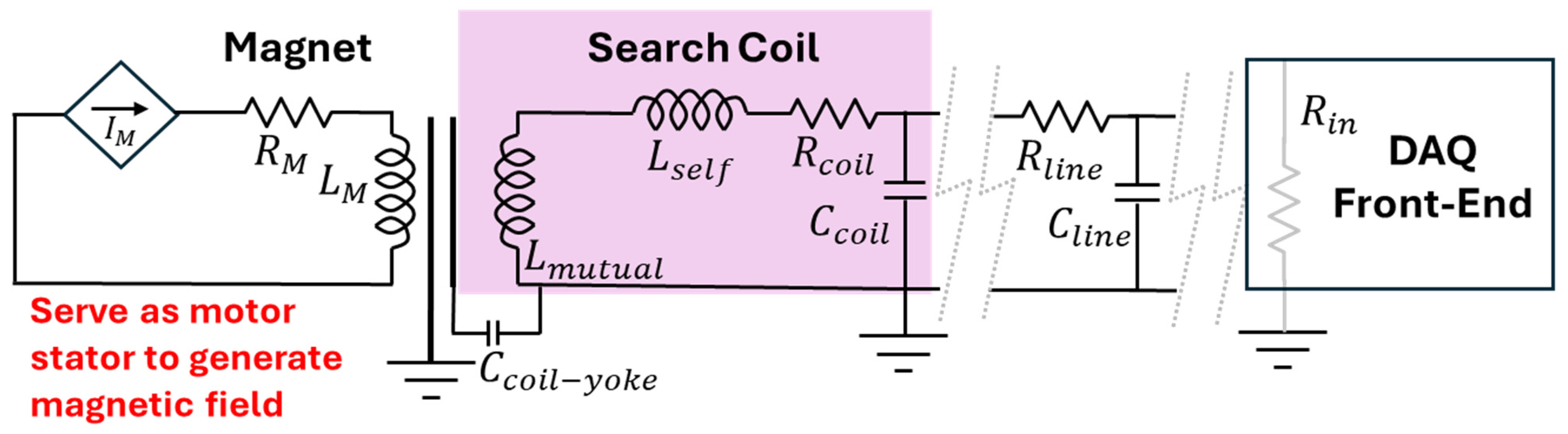
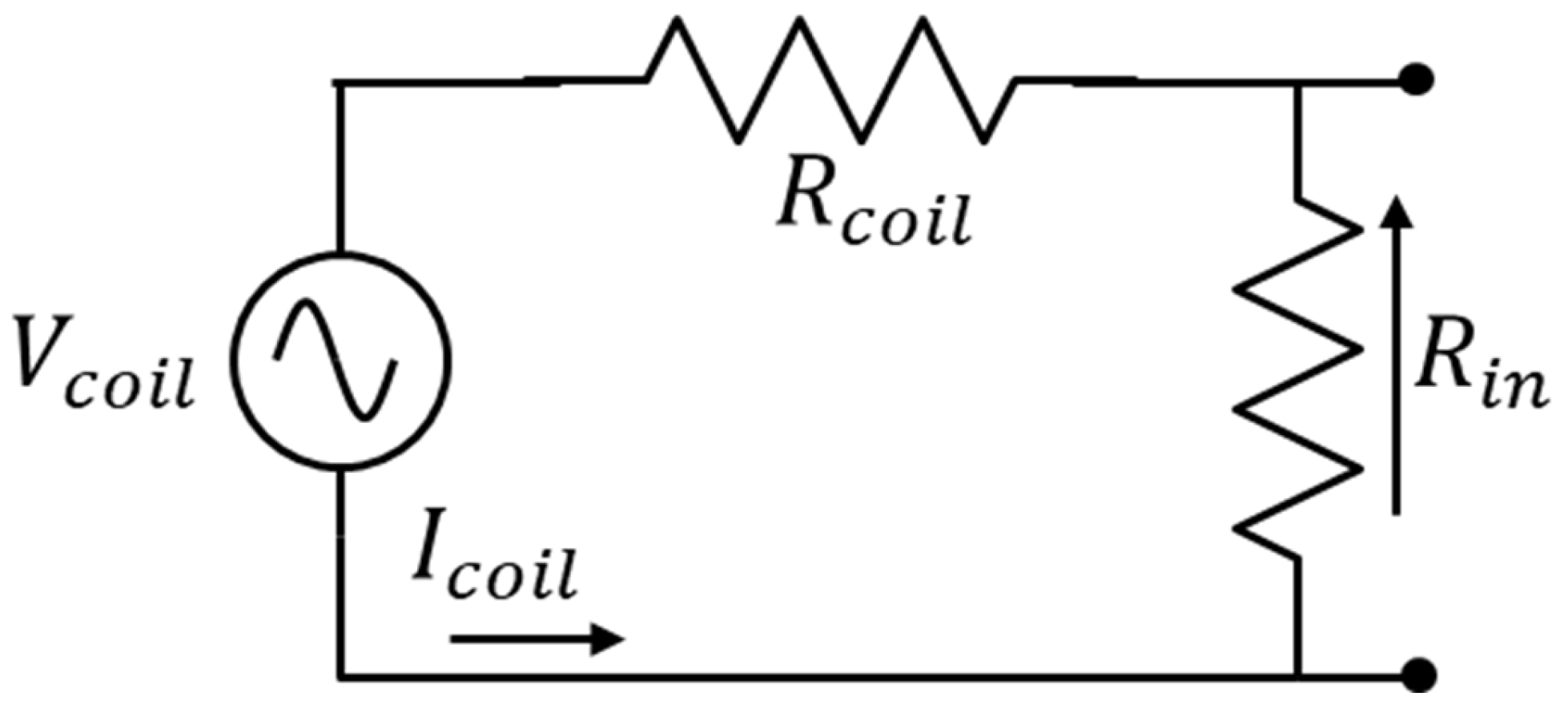
Figure 3 shows a search coil circuit model where the secondary winding of a transformer can be represented by the search coil, and the primary winding is the magnet generating the flux [32]. The output voltage of the search coil is fed to a data acquisition (DAQ) device through a transmission line, usually a coaxial cable, twisted pair, or insulated Litz wire. The DAQ device is designed to have a very high input impedance to minimize the circulating current in the coil. The complete circuit model as in Figure 3 is unnecessary in most practical cases if spectral content remains sufficiently below the resonant frequencies, typically for low-frequency approximation, that is, below 100 kHz [32]. So, the magnet coupling is replaced by a simple AC voltage source as shown in Figure 4 and the only important parameters are the coil resistance and the input impedance of the DAQ. The resulting parasitic current, $I_{coil}$ and the coil output voltage, which is the input voltage $V_{in}$ to the DAQ are given by (6) and (7) respectively.

$$I_{coil}={\displaystyle \frac{V_{coil}}{R_{coil}+R_{in}}}$$

(6)

$$V_{in}={\displaystyle \frac{1}{1+\frac{R_{coil}}{R_{in}}}}{V}_{coil}$$

(7)

$\mathrm{w}\mathrm{h}\mathrm{e}\mathrm{r}\mathrm{e}$ the input resistance $R_{in}$ of the DAQ are usually in the range of 10⁶ Ω, the parasitic current $I_{coil}$ in the order of 10⁻⁶ A, the coil resistance $R_{coil}$ in order of a few ohms, the induced voltage $V_{coil}$ depends on the search coil sensor sensitivity.

Due to the resistance of the coil and the DAQ, the measured voltage is smaller than the actual induced voltage by the factor, $k=1+R_{coil}/R_{in}$, which must be considered where high sensor design accuracy is required.

3. Proposed New Technique for Machine Diagnostics

3.1. Experimental Setup

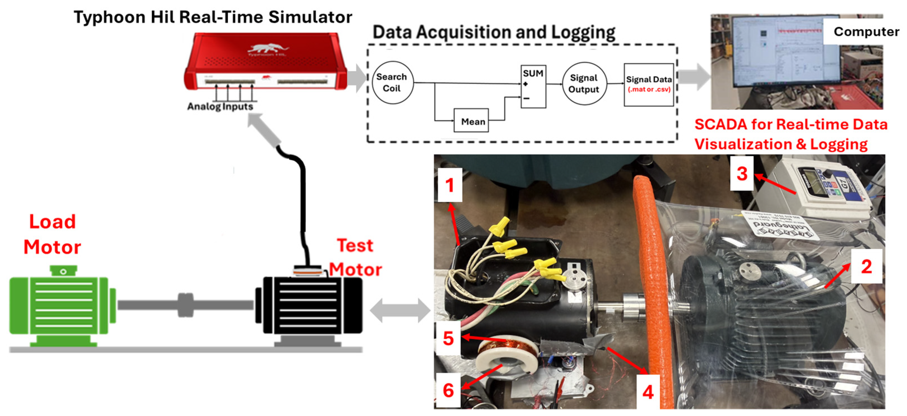
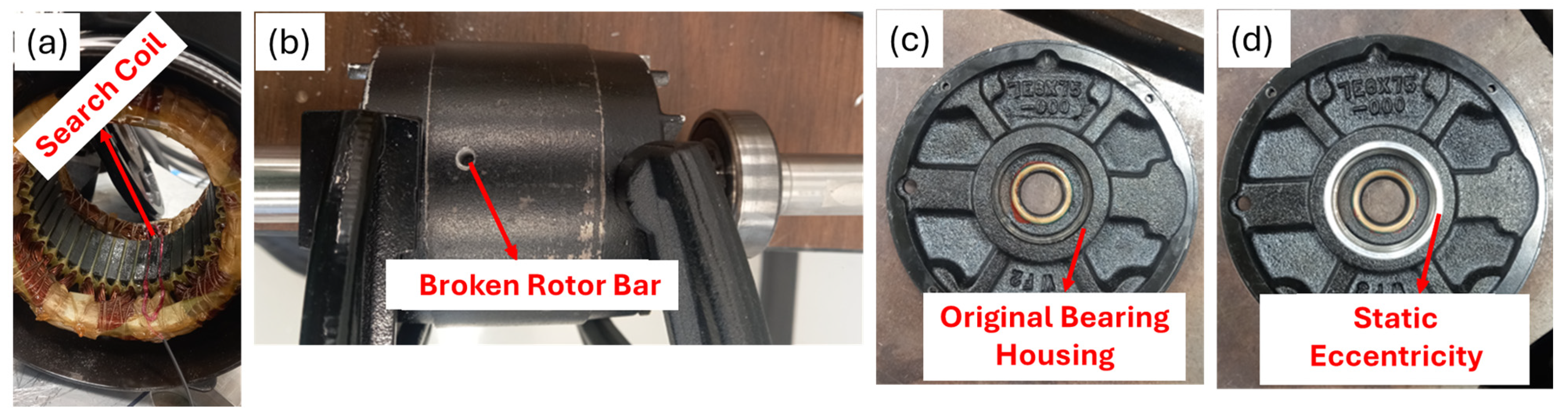
Figure 5 shows the electric motor test rig setup with magnetic flux measurements, using a search coil and stray flux sensors. A 460 V, 0.75 hp, 1725 rpm AC induction type is coupled with a load motor through an elastic coupling and tested under healthy conditions and different electrical defect conditions, including eccentricity, unbalanced supply voltage, broken rotor bar, and stator winding issues. For each condition, the two flux sensors (search coil and stray flux sensors) were installed in the positions shown in Figure 5. The machine was tested at no load and with varying loads using a Toshiba G7 variable torque control drive. The stray flux was measured with a 1500-turn enameled copper flux sensor of 0.274 mm wound around a circular former with a ferrite core flux concentrator installed on the frame (see Figure 5) with a sensor area of 0.01005 ${\mathrm{m}}^2$. The sensor can detect weak fields as low as 2 × 10⁻⁵ nT and the upper limit depends on the resonant frequency of the search coil. The coil sensor without an additional circuit is considered as an RLC circuit, the resonance can occur at a frequency $F_r$ expressed as $F_r=1/(2\pi \sqrt{LC}),$ where $L$ is the inductance of the sensor and $C$ is the parasitic capacitance. This sensor has a resonance at approximately 55 kHz, which means that the range of the sensor must be far from this frequency. In this study, the fault-sensitive harmonic frequency depends on the characteristics of the machine. Taking into consideration that the harmonics of interest for induction motors are in the lower frequency range (less than 1 kHz), the airgap flux was measured with a 10-turn enameled copper search coil of 0.193 mm placed on one of the stator’s teeth, as shown in Figure 6a.

The induced voltage from the stray flux sensor and search coil is acquired at a sampling frequency of 10 kHz using a Typhoon Hil 402 as a DAQ device [22]. The acquired data is then processed using Python 3.11 to develop machine-learning algorithms on a desktop computer.

3.2. Lab-Scale Fault Creation

The experimental setup is designed to investigate various electrical fault conditions of electric motors (healthy condition, eccentricity, unbalanced supply voltage, broken rotor bar, and stator winding issues), since the proposed new technique is data-driven and requires large, labeled datasets to achieve high accuracy and generalization. The airgap search coil for the magnetic flux measurement is installed as shown in Figure 6a. Lab-scale faults were created to mimic the real fault data, which are scarce from industry data captures. The rotor bar fault was introduced by drilling a hole in the rotor bar near one of the end rings, as in Figure 6b. For eccentric fault conditions, eccentricity (static eccentricity) is implemented by widening the one end bell of the bearing housing eccentrically and introducing a 0.23 mm off-center between the housing and the bearing, as in Figure 6d and the original bearing housing in Figure 6c.

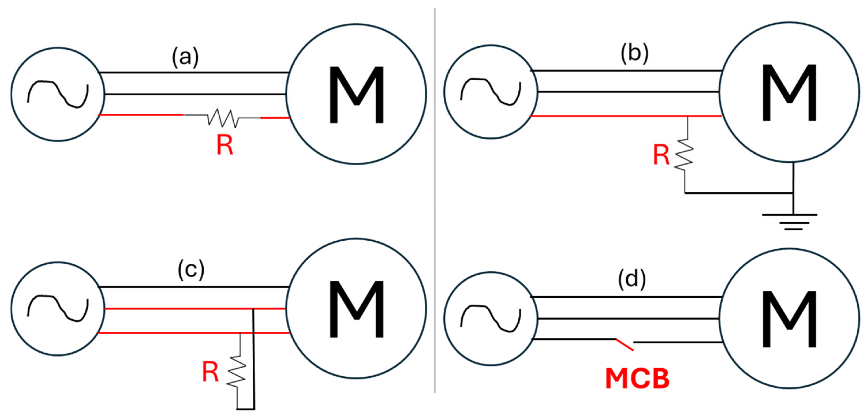
The unbalanced supply voltage fault was introduced by connecting a 10 ohm 450 watt power resistor between the grid supply and one of the motor supply terminals, as shown in Figure 7a to introduce an unbalanced voltage of about 2.81%. The stator winding faults are introduced as shown in Figure 7b–d, showing phase-to-ground and phase-to-phase faults respectively. The goal of a phase-to-ground stator winding fault is to introduce leakage from one phase of the motor frame. This is introduced by connecting one phase to the motor frame through a power resistor of 150 ohms, 1750 watts, as shown in Figure 7b. This introduced a leakage current of about 0.91 amps. For a phase-to-phase winding fault, the same power resistor is connected between two terminals of the motor, as shown in Figure 7c. Finally, an open-winding fault was created by disconnecting one motor terminal phase through an MCB while the motor was running to simulate a single-phased open-winding failure, as shown in Figure 7d.

3.3. Data Preparation and Transformation for ML Algorithms

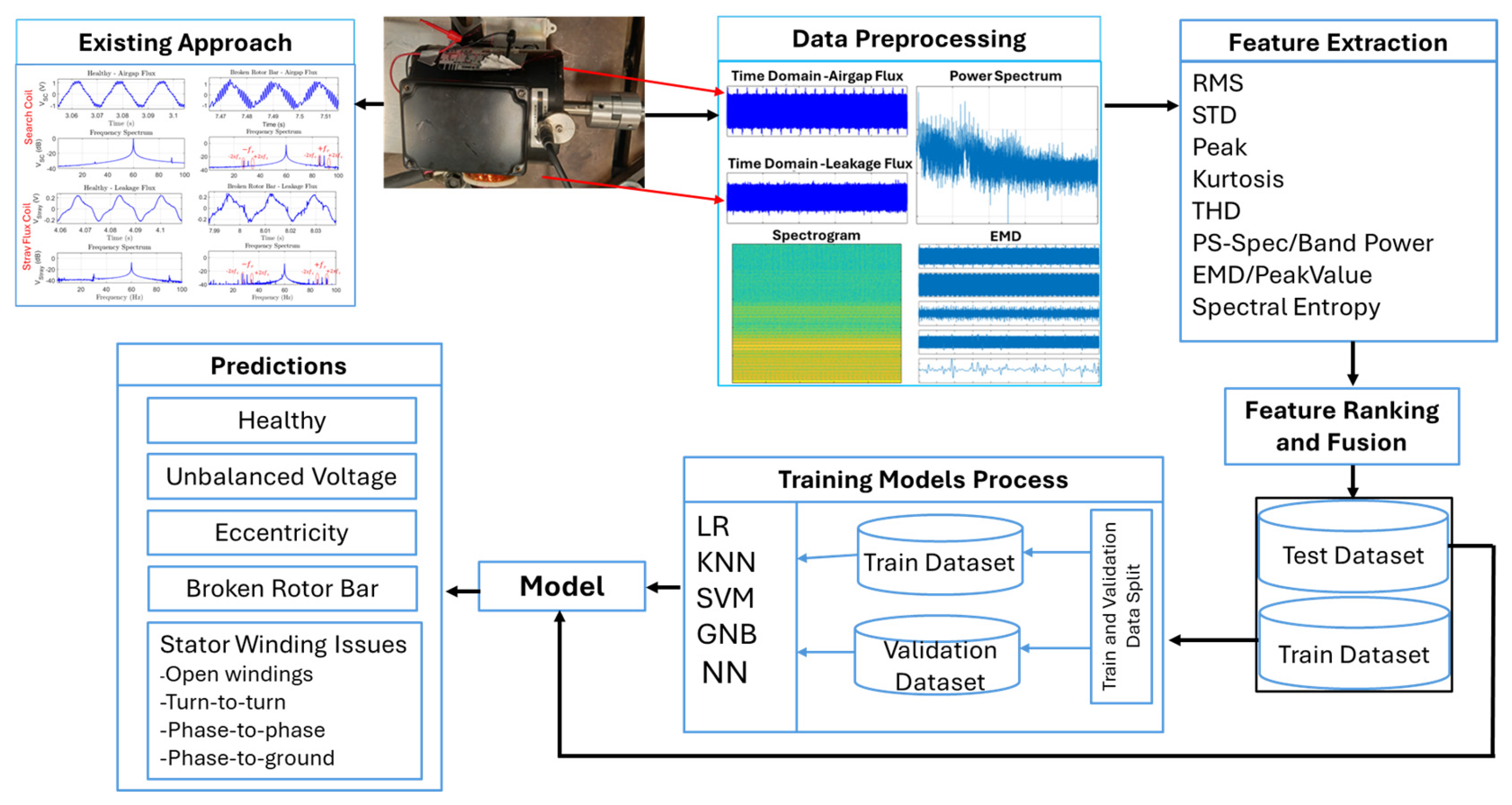
Many existing methods for diagnostics use FFT-based analysis of the airgap and leakage flux, which relies on frequency sideband identification as shown on the far-left side of Figure 8. These traditional methods can be significantly enhanced with ML techniques. ML is a branch of AI that enables computers to learn from data and make decisions without explicit programming. Applying trained ML models to larger flux data uncovers hidden insights, identifies trends, and predicts outcomes [33,34]. ML models were developed for condition-based monitoring (CBM) of induction motor fault detection and diagnosis using magnetic flux data from various operating conditions, as shown in Figure 8. The airgap flux and leakage flux datasets were recorded for 10 seconds at a frequency of 10 kHz for 836 samples with 100,000 data points. Flux data can offer unique insights to inform ML systems through signal processing, such as time domain, FFT, and other advanced signal processing—power spectrum (PS), spectrogram, and Empirical Mode Decomposition (EMD).

3.3.1. Data Preprocessing and Feature Engineering

Data preprocessing refers to the transformation and formatting of raw data into a data ensemble suitable for machine learning. A data ensemble is used to combine data from multiple sensors for organizing and managing multifaceted datasets, thereby improving performance, reliability, or insight. The time-domain flux datasets are put into an ensemble table to create a data timetable and fault label. The time-domain technique for detecting trends to predict faults has been presented in many literature sources [1,35]. A comparison with traditional signal processing methods, using the Fast Fourier Transform (FFT), for fault detection and diagnosis is discussed in many published papers. Also, fault detection, using EMD was discussed extensively in references [34,36].

Power Spectrum (PS) characterizes a system’s frequency content and resonances. Electric machine degradation usually causes changes in the spectral signature. Power spectral density (PSD) is a representation of a signal’s energy or power distribution across different frequencies. PSD is a significant tool for signal processing applications in electric machine diagnosis.

Let $x(k)$ be a discrete signal with expected mean $(E)$. The power spectral density of $x(k)$ is defined as the Discrete FT of the autocorrelation sequence [37]:

$$S_{xx}(f)={\sum }_{k=-\infty }^{\infty }{R}_{xx}(k)e^{j2\pi fk}$$

(8)

The power spectral density of $x(k)$ is defined as the Discrete Fourier Transform (DFT):

$$S_{xx}(f)=E\{\left|{X(f)}^2\right|\}$$

(9)

$\mathrm{w}\mathrm{h}\mathrm{e}\mathrm{r}\mathrm{e}$ $f$ denotes the frequency bin, $k$ is a discrete time delay.

$$X(f)={\sum }_{k=0}^{N-1}x(k)e^{-j2\pi fk/N}$$

(10)

$R_{xx}$ is the autocorrelation function, $N$ is the number of samples, $k$ is the frequency bin.

A spectrogram is a visual representation of the frequency content of a signal over time, enabling the analysis of how a signal’s spectral properties change over time. This is done by dividing the signal into segments of length M, known as windows. The spectrogram, a time-frequency representation of the signal, is the magnitude squared of the Short-Time Fourier Transform (STFT). From Ref. [38], the STFT of a discrete signal is a sequence of DFTs computed over short, overlapping windows of the signal, as given by

$$X_m(f)={\sum }_{k=-\infty }^{\infty }x(k)g(k-mR)e^{-j2\pi fk}$$

(11)

$\mathrm{w}\mathrm{h}\mathrm{e}\mathrm{r}\mathrm{e}$ $g(k)$ is the analysis window of the $M$ signal length, $R$ is the hop size, and m is the frame index.

$$spectrogram=\left|{X_m(f)}^2\right|$$

(12)

3.3.2. Feature Selection and Extraction

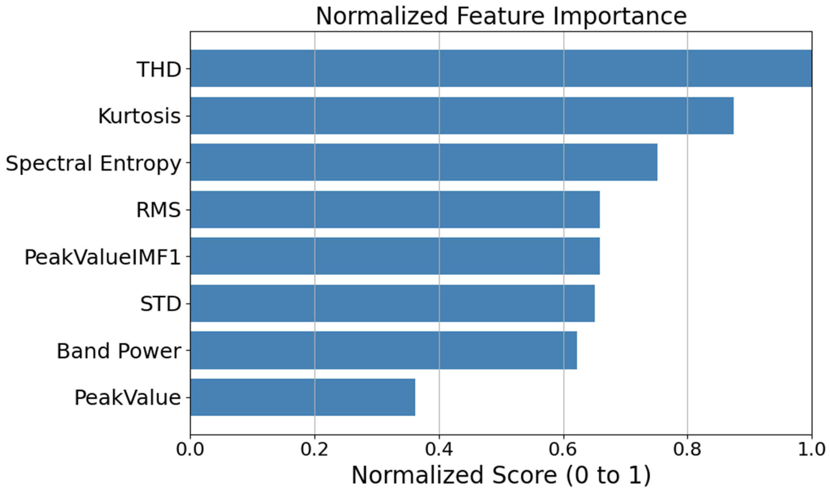
Distinct feature extraction is a crucial step in many ML models, aiming to reduce vector dimensionality, enhance interpretability, and improve model performance. There are many methods of feature selection and extraction, model-based feature-importance [39], principal components analysis [40], linear discriminant analysis [41], and autoencoder [42], but the method that is used depends on the ML-designed application. In this study, we used model-based feature importance for feature selection. The flux data from airgap and leakage flux sensors installed in the IM under test are preprocessed to identify correlations between specific patterns of machine conditions. The time domain features, such as RMS, STD, THD, and peak value, are statistically extracted, while spectral features are extracted using the PS, spectrogram, and EMD algorithms. The most distinct features like kurtosis, spectral entropy, THD, peak value, RMS, STD, band power, and peak value of the first intrinsic mode function (PeakValueIMF1) for each motor condition, are extracted. We extracted the same set of features for both the airgap flux and leakage flux. Figure 9 shows a horizontal histogram plot, known as ranked normalized feature importance, that indicates how much a feature contributes linearly to the probability class based on model weights. The extracted features serve as input to ML models for model training.

3.4. ML Classifiers

In this study, we evaluated classifiers commonly used in machine learning, including logistic regression (LR), K-nearest neighbor (KNN), support vector machine (SVM), Gaussian naïve Bayes (GNB), and neural network (NN). These classification algorithms are supervised learning approaches that aim to predict the class of instances based on their features and understanding of complex datasets. The classification algorithm involves training a model on a dataset that has already been labeled with classes or fault codes and then using the trained model to classify new, unseen instances based on the predefined fault categories. So, a good classifier should be able to give good accuracy outside of training datasets, fast training, and fast testing, while explaining the facility, that is, generates rules after training or state limitation(s). The mathematical models of each ML algorithm, including LR, KNN, SVM, NN, and GNB, are well known and detailed in references [1,22,35,37,43].

3.5. Deep Learning Models

A major challenge in applying ML to modern electric machine diagnostics is the lack of transferability. Models trained on one machine often fail when applied to another machine due to structural differences (such as slot, pole design, and rotor geometry) and operating conditions (including load, slip, and noise). This lack of transferability severely limits the industrial applicability of ML-based diagnostic methods. To address this drawback, a generalized model for an advanced and improved electric machine diagnostic system that can learn transferable fault representations across machine types needs to be developed.

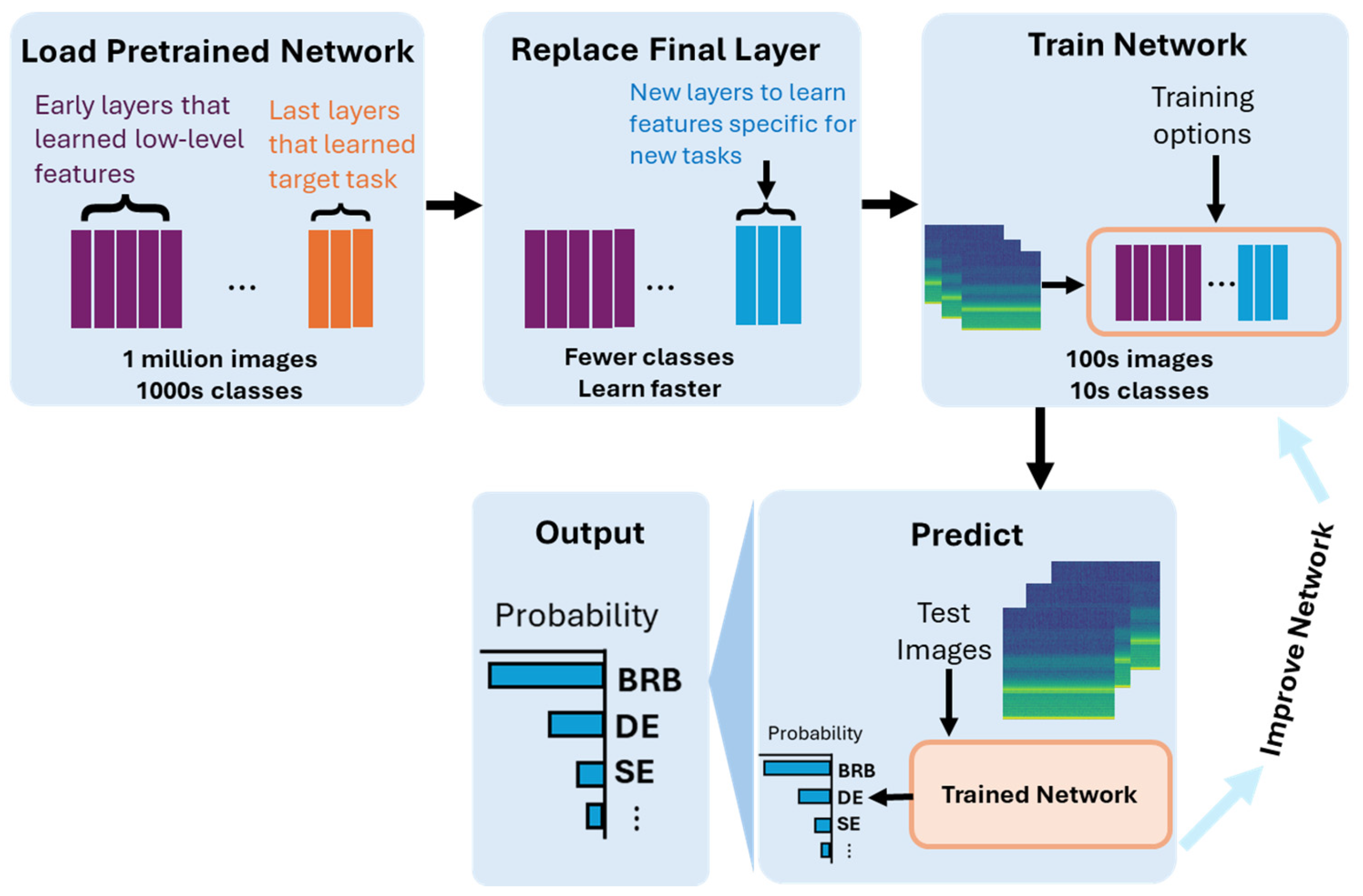
CNN is an advanced version of artificial neural networks (ANNs), particularly useful for visual datasets like images or videos, and primarily designed to extract features from grid-like matrix datasets. Many CNN classification approaches for fault diagnosis have been used in the literature [44,45,46], but all lack demonstration of generalization across different machine types. Hence, it does not demonstrate the knowledge transferability of the trained model. As the convolutional layers increase in depth to develop a more robust deep learning architecture, CNNs experience vanishing or exploding gradients. Hence, there is a need for the development of deep CNN pretrained models. Self-supervised pretraining enables learning generalizable representations from large unlabeled datasets across multiple machine domains. The pretrained models are fine-tuned with small, labeled sets from new machine dataset to improve adaptability, as shown in Figure 10. These pretrained models are initially trained with enormous amounts of datasets like ImageNet [47]. Most of the ImageNet pretrained models are developed from a convolutional neural network (CNN) as a building block. The performance of these models varies depending on the architecture and consists of multiple layers that progressively extract features from the input images and transfer low-level features learned to the new task.

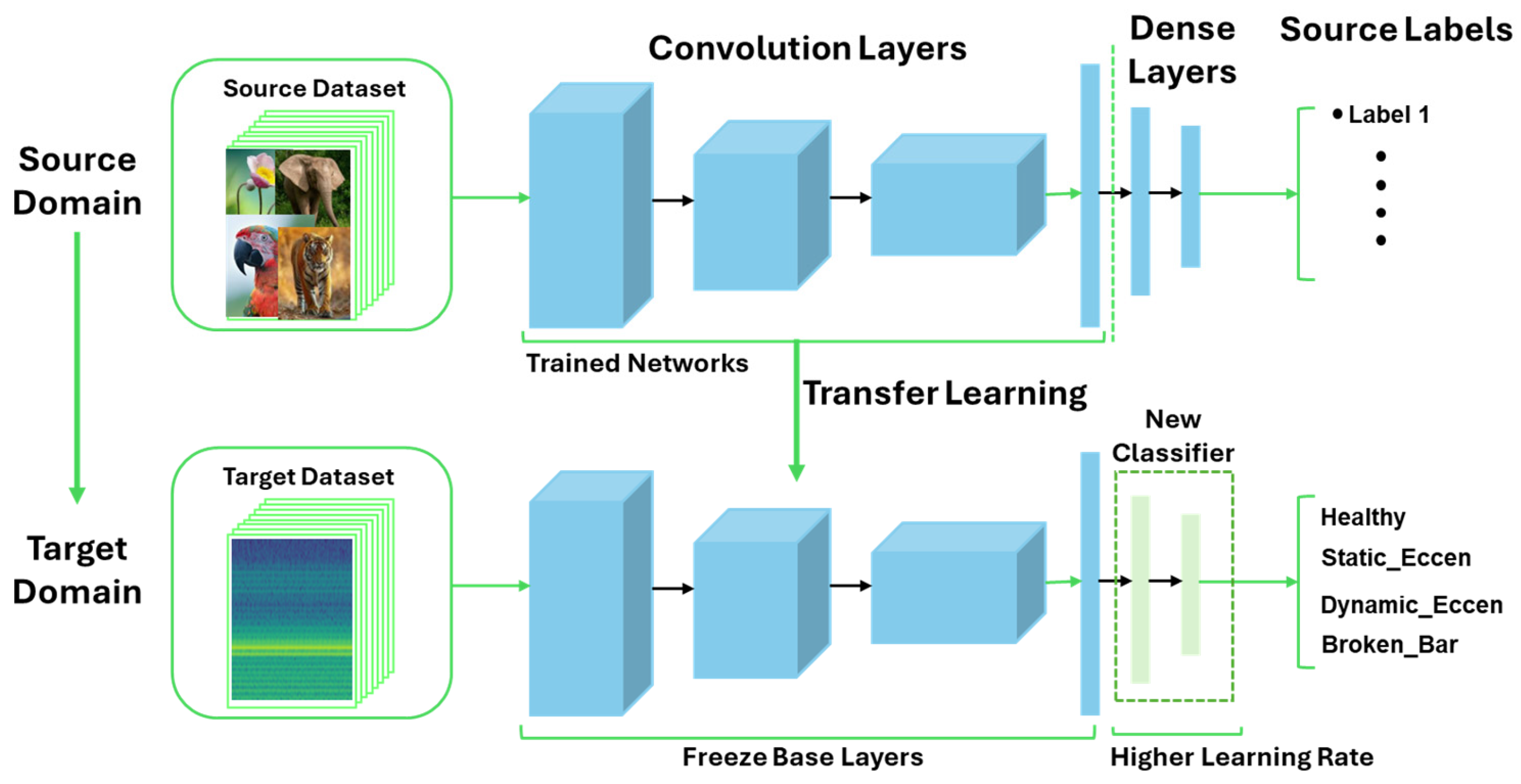
Transfer Learning (TL) is a machine learning technique in which a model trained for a specific task is reused as the starting point for a model on a second task. This technique is valuable when acquiring enormous amounts of labeled data for the new task is impossible, as in industrial settings, or computationally expensive. TL relies on three key concepts: pretrained models, feature extraction, and fine-tuning [47]. Pretrained deep neural networks have been trained on vast datasets for a specific task and learned robust and generalizable features in their early layers, which can be helpful for related problems [48]. The early layers of pretrained models, which learn low-level features such as edges and textures in an image, are typically used as a fixed feature extractor. The output of these layers serves as input to a small network that is specifically trained for a target task. Finally, the pretrained model can be fine-tuned by unfreezing some or all its layers, often with the learning rate and classifier output as shown in Figure 11. In this study, TL with fine-tuned deep convolution neural networks CNN ImageNet models in MATLAB version 2024a software, Google Net, Inceptive-v3, ShuffleNet, MobileNet-v2, ResNet50, and DenseNet is used for electric machine fault diagnosis using magnetic flux measurements that are transformed into spectrogram images. To train for the target domain, the approach is to freeze the convolution layers of the pretrained model and adjust the input image size to match pretrained CNN ImageNet models, maintaining the same weights used during the ImageNet training since the model has learned from the previous training. The final layers of the pretrained model are removed and replaced with the dense layers for the target domain, fine-tuned by adjusting the number of classes to four (4) (classifying four motor operating conditions instead of 1000 general object categories with a higher learning rate of 10 times the learned convolutional layers. The new layers contained in the target datasets are trained to learn task-specific patterns of classifying BRB, DE, H, and SE.

4. Results and Discussion

4.1. ML Model Performance and Limitations

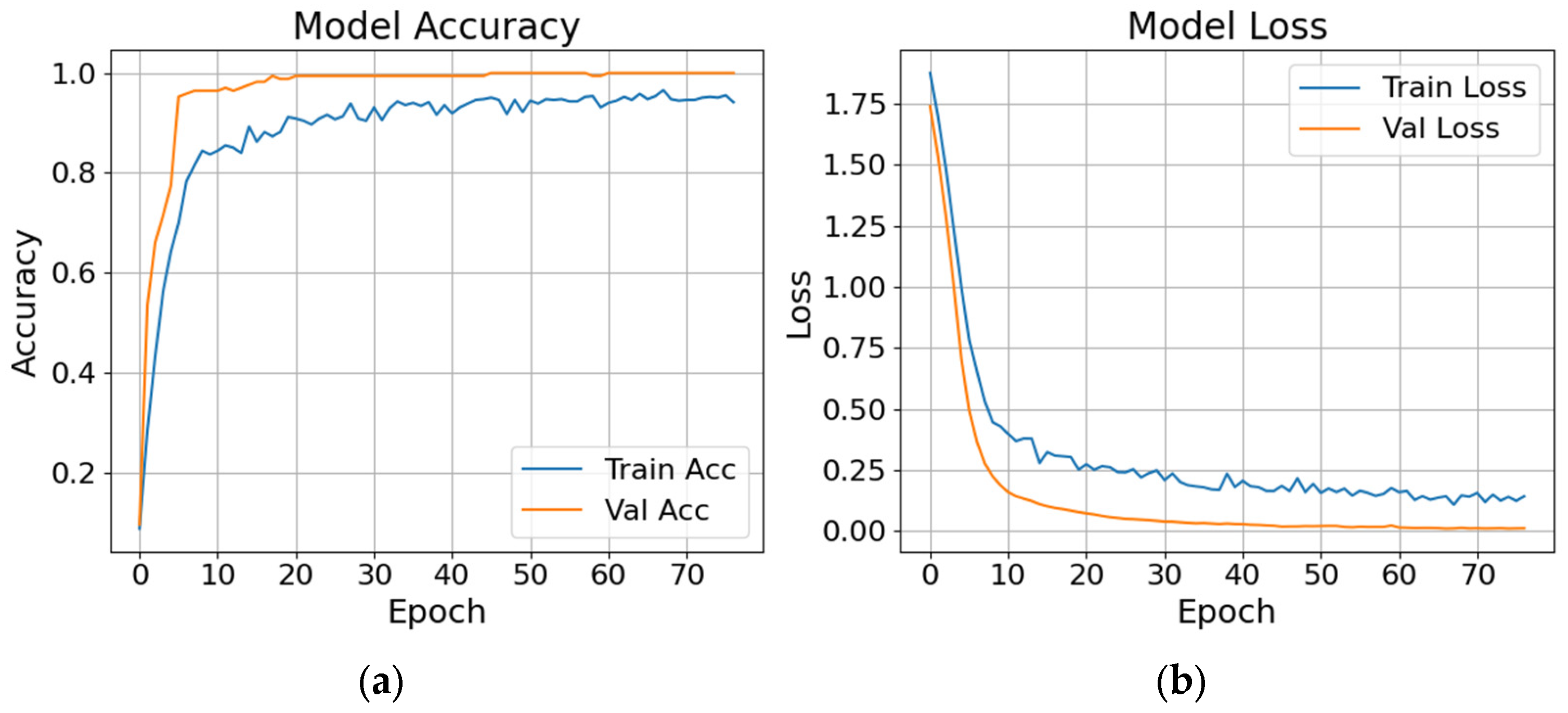
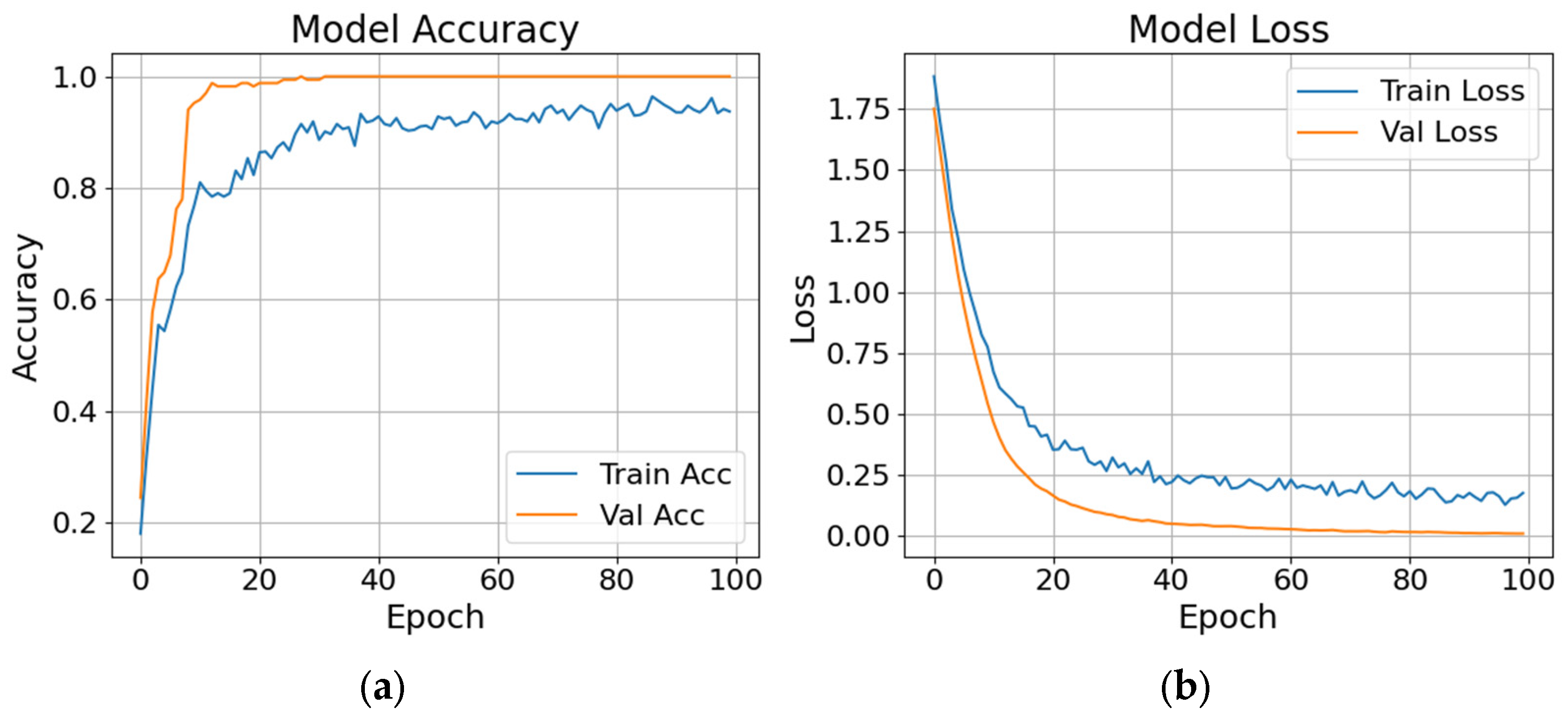
Five machine learning models were developed to classify fault conditions in an electric machine using seven statistically and signal-derived features, as demonstrated earlier. The dataset (BU datastore) consists of 836 labeled samples (approximately 120 samples per class), covering seven distinct operating conditions, including healthy (H), BRB, SE, unbalanced supply voltage (USV), phase-to-phase (PPSC), phase-to-ground (PGSC), and open-circuit faults (OC). The models, LR, SVM, KNN, GNB, and NN, were trained and evaluated on the same standardized dataset using an 80/20 train/test split [1]. The performance metrics were based on test data. The main parameter for each of the statistical ML (LR, SVM, KNN, and GNB) models shows that the NN model was optimized, and grid search was used to obtain the number of hidden layers and neurons that give the maximum performance without model overfitting. For the NN trained on the airgap flux, two hidden layers with 16/12 neurons were used, while only one hidden layer with 8 neurons was used for training the NN for the leakage flux [1]. The model overfitting was avoided by implementing 10% dropout and 5 validation patience, known as early stopping, during the training process. After the training, all the statistical classifier trained models, LR, SVM, KNN, GNB, were able to generalize 100% of our unseen dataset of the same motor for airgap and leakage flux datasets. On the generic neural network trained models, the model trained with airgap flux features generalized up to 99.40% and 100% on the leakage flux features, as shown in Figure 12 and Figure 13.

Table 1. Performance of the trained NN (airgap flux) model on unseen dataset.

	BRB	H	OC	PGSC	PPSC	SE	USV
BRB	1.00	0.00	0.00	0.00	0.00	0.00	0.00
H	0.00	1.00	0.00	0.00	0.00	0.00	0.00
OC	0.00	0.00	1.00	0.00	0.00	0.00	0.00
PGSC	0.00	0.00	0.00	1.00	0.00	0.00	0.00
PPSC	0.00	0.04	0.00	0.00	0.96	0.00	0.00
SE	0.00	0.00	0.00	0.00	0.00	1.00	0.00
USV	0.00	0.00	0.00	0.00	0.00	0.00	1.00

and

Table 2. Performance of the trained NN (leakage flux) model on unseen dataset.

	BRB	H	OC	PGSC	PPSC	SE	USV
BRB	1.00	0.00	0.00	0.00	0.00	0.00	0.00
H	0.00	1.00	0.00	0.00	0.00	0.00	0.00
OC	0.00	0.00	1.00	0.00	0.00	0.00	0.00
PGSC	0.00	0.00	0.00	1.00	0.00	0.00	0.00
PPSC	0.00	0.00	0.00	0.00	1.00	0.00	0.00
SE	0.00	0.00	0.00	0.00	0.00	1.00	0.00
USV	0.00	0.00	0.00	0.00	0.00	0.00	1.00

show the trained NN model performance on the unseen dataset for airgap and leakage flux models, respectively. Table 1 and Table 2 show the NN trained model performance on test data in a confusion matrix in a table form. The trained models on both airgap and leakage flux features exhibit superior generalization across all fault classes on the same motor type, consistently achieving remarkably high accuracy regardless of the algorithm used.

Since extracted features are statistically evaluated, a change in motor type affects the features used in ML model training. Without retraining the models, previously trained ML models often fail due to structural differences, power ratings and/or operational conditions. To prove this, the trained model with the BU dataset was applied to a dataset from another researcher (External dataset) to determine whether the trained model could accurately predict or classify the fault conditions in the foreign dataset. The dataset from the foreign lab is described in Section 4.2 and the results are shown in Section 4.3.

4.2. Magnetic Flux Sensor Data from Other Research Lab [5]

The foreign or external dataset used for ML trained model evaluation is from Electrical Energy Conversion System Lab (EECSL), Korea University. The research Lab database contains measurements of seven different operating conditions (healthy, imbalance, misalignment, looseness, bearing defect, eccentricity, and broken rotor bar) from vibration and flux sensors installed on a 7.5 hp induction motor (IM). These faulty conditions were emulated [5] under changing load and frequency levels. Each recorded sample contains 512,000 data points and is sampled at 10,240 Hz (approximately 10 kHz). As it relates to the trained model, the steady state airgap flux signal operating at rated conditions (60 Hz and full load) under healthy (H) and broken rotor bar (BRB) conditions is downloaded so that the datasets are processed further before ML model performance evaluation on external data.

The authors downloaded two samples, one for H and the other for BRB, since the two are the only fault scenarios same as in the BU dataset to train NN model. Then, data engineering was conducted to transform each of the sample data length into 10 samples by developing a data chunk algorithm in MATLAB software since the downloaded datasets are in MATLAB files and resampled at exactly 10 kHz. After passing through our chunk algorithm, one set of the Korea lab’s data sample for H was divided into 10 samples and the resulting data points were 51,200 for each sample. The same approach was used to create 10 samples for BRB. The created 20 chunk samples are then preprocessed to extract the same statistical features used during NN model training and the extracted features are used to test NN trained model performance. The predicted model performance results are shown and discussed in Section 4.3.

4.3. Neural Network Model Result of External Data from Other Research Lab

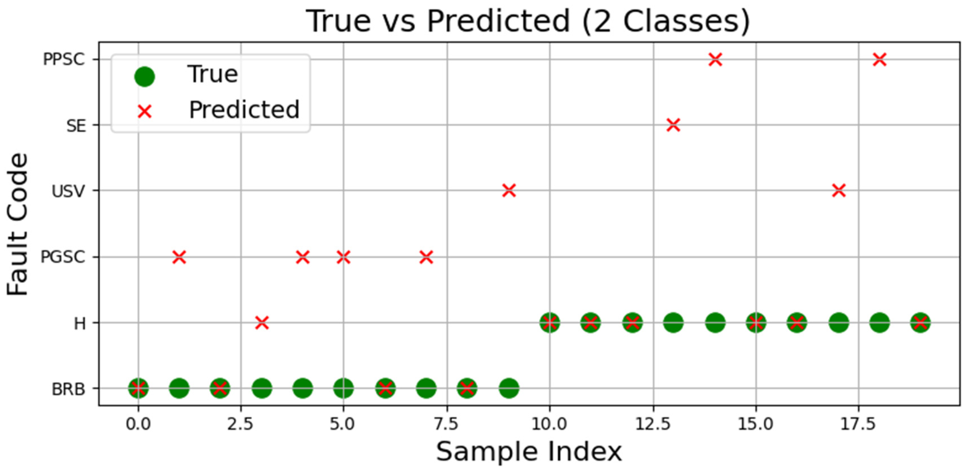
Figure 14 shows the result obtained when an NN model previously trained with airgap features extracted from the author’s test motor is tested on airgap features from the data from the external research lab described in Section 4.2. Note that the rated power of our lab test motor is 0.75 hp while that of the external lab is 7.5 hp. In Figure 14, the predicted cases are shown with an asterisk, and the actual fault state is shown with a green dot. It is observed that for the broken rotor bar fault (BRB), six fault states were misclassified; four states as phase-to-ground short circuit fault (PGSC), one as healthy (H) and the other as unbalanced supply voltage (USV). For a healthy (H) machine, four states were misclassified, with two as phase-to-phase short PSC), one as static eccentricity (SE) and another as unbalanced supply voltage (USV). Thus, for 10 samples of BRB and 10 samples of H, totaling 20 samples, only 10 were correctly predicted (or about 50% accuracy), proving that the trained model from one dataset can generally not be transferred to other data without retraining. This lack of transferability or generalization severely restricts the ML diagnostic approaches since it is impractical to retrain models for every new machine type. The proposed solution to overcome this challenge is presented in Section 4.4.

4.4. Fine-Tuned Deep CNN Models with TL

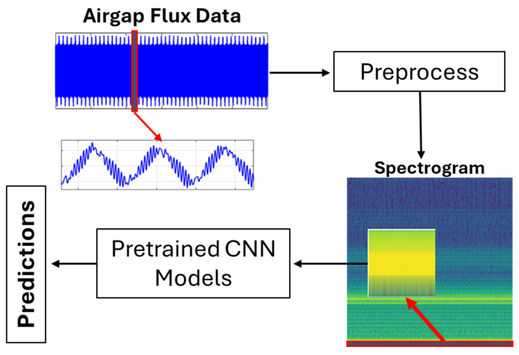
Having seen from the ranked feature importance in Figure 9, the spectral entropy from the spectrogram is an especially important feature to distinctly characterize the motor signatures under different operating conditions. A spectrogram is a visual representation of the frequency content of a signal over time, whose spectral entropy indicates degree of randomness and is more prone to faults. The spectrogram was chosen for the development of a deep CNN fine-tuned pretrained model for an improved diagnostic framework because it transforms a 1D flux signal into 2D time-frequency representations (image), which allows the CNN to leverage spatial patterns, textures, and harmonic structures for accurate fault classification or prediction in flux analysis. The feature representation of a spectrogram captures both harmonic and temporal information, making it ideal for complex signal analysis in tasks like machinery fault detection. To distinctly classify the fault conditions, the time domain signals acquired from the magnetic airgap flux sensor under healthy, broken rotor bar, and static eccentricity from our dataset, only the dynamic eccentricity fault condition from the external dataset is created as a datastore for deep CNN model training. The DE fault conditions can be created by machining the motor shaft and precisely inserting an off-centered sleeve to emulate the DE fault, but there is a synthesis of the DE of the external dataset source with noise. The DE external dataset was synthesized with 40 dB SNR Gaussian noise to create entirely new datasets, both of which will appear on the model as different datasets. The time domain data are preprocessed to maintain the same 51,200 data points at a sample rate of 10 kHz for all the samples and then transformed into spectrogram images, limited to 0–120 Hz where most of the fault harmonics are expected to appear. This process was also repeated in preparing the external dataset before transforming it into a spectrogram image for the model testing. The section of the spectrogram image, as shown in Figure 15, serves as the input to the deep CNN models trained with TL. The output of these models was fine-tuned to match the number of classes of the new dataset and freeze all convolutional layers to maintain ImageNet trainable weights. So, only the dense layer, which is our new classifier, is trained. A total of 100 image samples are used for each operating condition for the training, of which 15% is for model evaluation.

The pretrained CNN ImageNet classification models have already learned to extract powerful and informative features from natural images; therefore, TL could be applied to fine-tune to learn features specific to new tasks. The knowledge learned during the initial training is transferable to a small set of new data. However, the high accuracy or cross-domain generalization does not always transfer directly to new tasks, so it is a good practice to try multiple models to select the most suitable for a given application. We investigated the following popular CNN pretrained models: GoogleNet, Inceptive-v3, ShuffleNet, MobileNet-v2, ResNet50, and DenseNet-201. Each has a different layer depth and trainable parameters. We used Adam as the optimization algorithm that updates weights to minimize loss, maximum epochs of 8, batch size of 11, and stopping criteria of 5.

Table 3. Transfer learning CNN models’ performance.

Pretrained Neural Network Models						Trained Models’ Performance
S/N	Neural Network Name	Depth	Size (MB)	Parameters (Millions)	Image Input Size	Model Size (MB)	Accuracy (BU Data)	Accuracy (External Data)
1	GoogleNet	22	27	7	224-by-224	21.71	75	25
2	Inception-v3	48	89	23.9	299-by-299	77.60	100	67.5
3	ShuffleNet	50	5.4	1.4	224-by-224	3.31	100	75
4	MobileNet-v2	53	13	3.5	224-by-224	8.17	100	75
5	ResNet-50	50	96	25.6	224-by-224	85.77	100	100
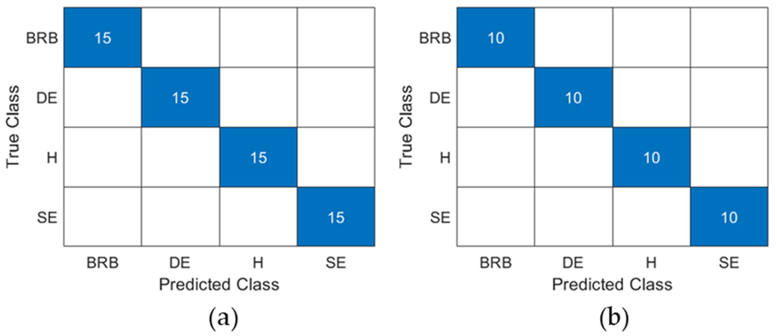
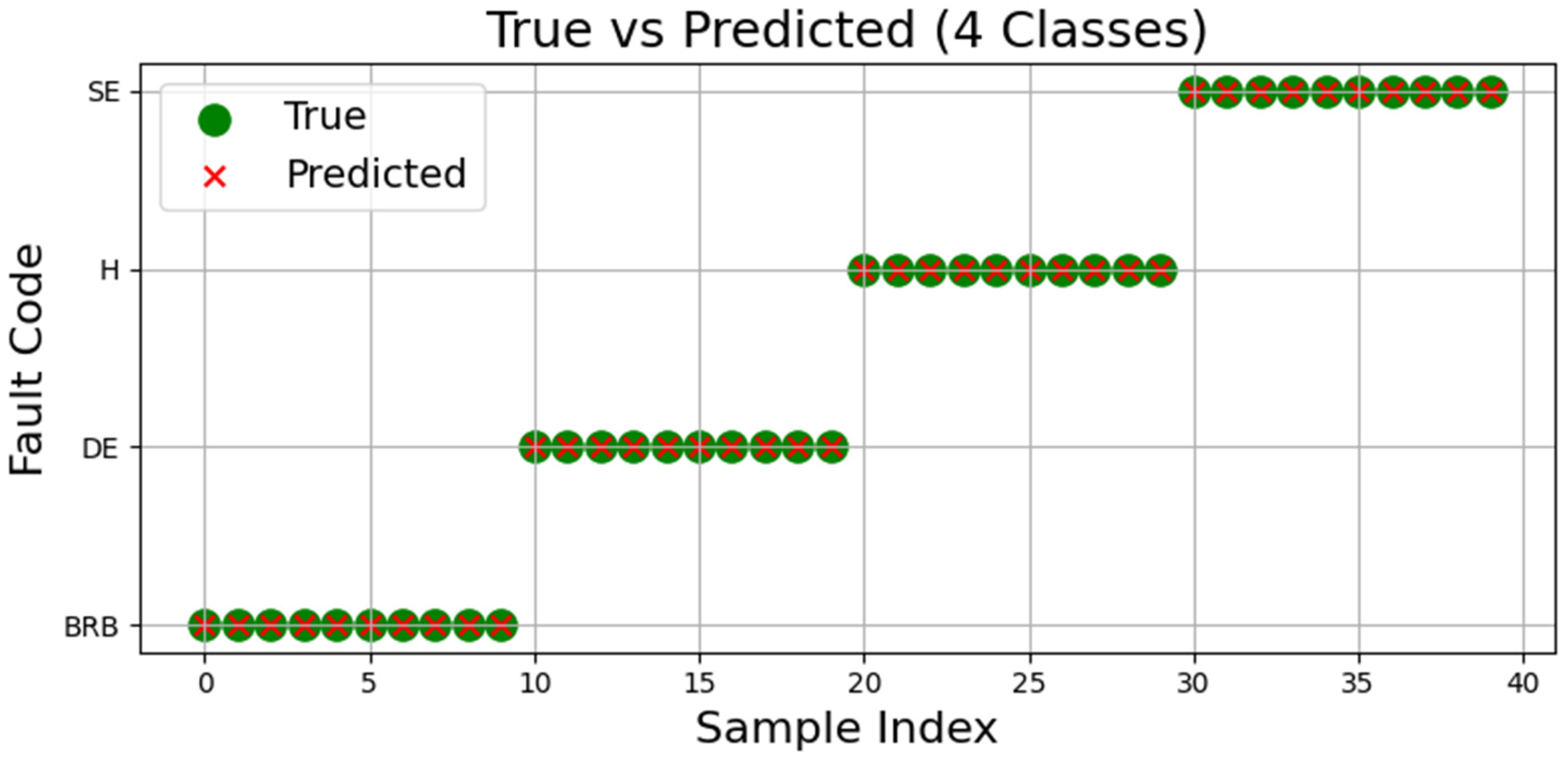
6	DenseNet-201	201	77	20	224-by-224	67.7	93.33	75

shows a performance comparison of the six developed pretrained models. The trained models were evaluated with our unseen test data (BU data) from 0.75 hp IM and with the external research lab’s dataset (External data) from a 7.5 hp IM [18]. It can be seen from Table 3 that the model’s performance is not dependent on the layer depth nor on the trainable parameters, but mainly on the architecture of the pretrained model. Considering the layer depths, one would expect DenseNet and MobileNet-v2 trained models to perform better than the ResNet50 model, but that was not the case, which confirms that the performance is heavily influenced by the network architecture. Hence, it is seen that the deep CNN ResNet50 model outperformed all other models. The ResNet50 model was able to generalize 100% on both BU data and the external data, as shown in Figure 16a,b, respectively. The performance improvement achieved with the deep CNN ResNet50 model is further elucidated in Figure 17 to show a contrast to Figure 14 described in Section 4.3. Figure 17 shows four classes of 10 samples per operating condition. The y-axis is the fault code, while the x-axis is the number of samples used for model testing. It is seen that the trained CNN ResNet50 model accurately predicted all four motor conditions.

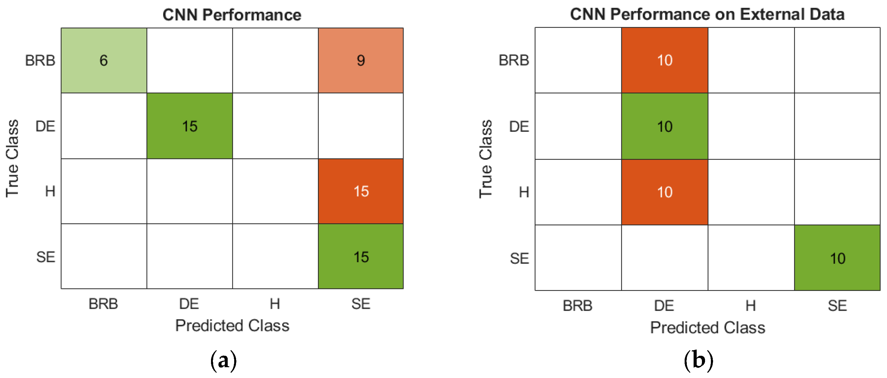
Before proceeding to the pretrained deep CNN models’ performance comparison, it will be good to also train a traditional CNN so that it can be compared with the best-trained deep CNN model to demonstrate its architectural capability. A custom traditional CNN consists of three convolution blocks, 3 × 3 kernels with 16, 32, 64 filters and each with batch normalization, ReLU activation, and 2 × 2 max pooling. The same training option used during pretrained CNN models is maintained. Figure 18a shows the traditional CNN performance on the unseen dataset (BU dataset) and Figure 18b shows the traditional CNN on the external dataset. It can be depicted from the plots that the traditional CNN model cannot be used for machinery diagnostics because it can only classify 60% and 50% accurately on the unseen dataset and external dataset, respectively.

The ResNet50 model is widely used in computer vision for image classification because of the features of its architecture: convolutional layers, batch normalization, and pooling [46]. It employs skip connections and bottleneck design to enhance efficiency. Skip connections are branches in the computational path that allow each network layer to be added back to the output. These connections enable gradients to flow directly through the network and prevent them from becoming negligibly small during training. This is to avoid vanishing or shattered gradients to allow more depth layers without overfitting [49]. On the other hand, the bottleneck design allows the output block to match the input dimension for the residual connection, thereby reducing the computational cost, learning abstract features effectively, and improving efficiency. These ResNet50 architecture designs are probably the main contributing factors that gave the trained ResNet50 model an edge over the other models shown in Table 3.

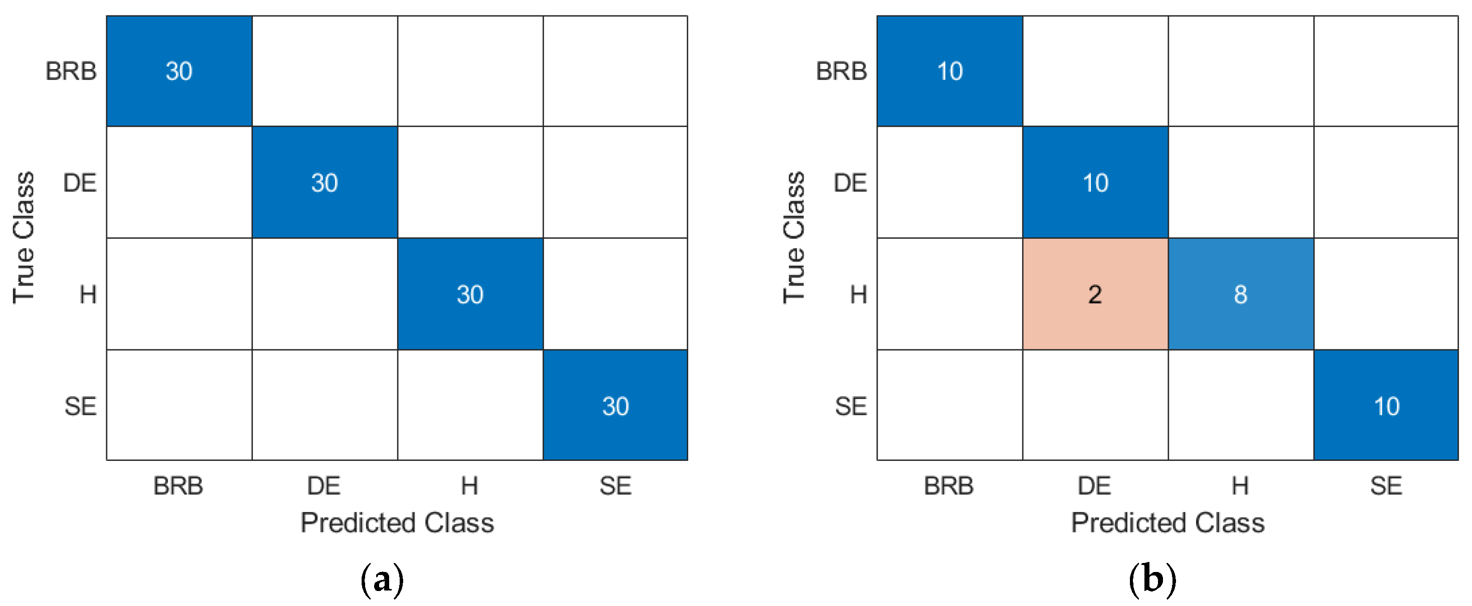
To demonstrate the ResNet50 model’s robustness with noise to emulate a noise environment and/or sensor degradation, another ResNet50 model is trained with 100 samples of BU data and 100 samples of BU data with the addition of low noise power of 40 dB SNR. ResNet50 demonstrates high robustness against noise as shown in Figure 19. The performance degrades under extreme noise, and its residual structure and deep extraction of its strength allow it to retain significantly higher accuracy. This fine-tuning of ResNet50 with noisy images allows it to learn robust patterns, enabling it to recognize fault states even when the input signal is heavily degraded. In this study, the noise injection technique used is Gaussian noise, which is the most commonly used for data augmentation to inject noise into the input data. This helps in reducing model overfitting. Gaussian noise has a zero mean and a controllable standard deviation that allows noise intensity adjustment and needs to be optimized. Figure 19a represents the model performance on BU data and Figure 19b represents external data performance, which is 100% for BU performance and 95% for external data.

5. Conclusions

Currently proposed ML-based diagnostic methods are faced with three critical issues: the presence of weak fault signatures, the scarcity of labeled data required for effective machine or deep learning models, and the lack of transferability of the diagnostic methods across machines regardless of the machine type, power rating or manufacturer. The existing ML models predict faults with extremely high accuracy on the same machine type but often fail when applied to another due to structural differences and operating conditions. This lack of transferability or generalization of ML models severely restricts industrial adoption of the ML diagnostic framework, hence the need for a robust, data-efficient, and transferable diagnostic framework is paramount. In this paper, an advanced diagnostic approach to address the issues is proposed through the integration of advanced signal processing techniques and machine learning algorithms to enhance fault diagnosis. Transfer learning (TL) techniques were utilized to train deep learning (DL) pretrained CNN models on spectrogram images of magnetic flux signals corresponding to different operating conditions (H, BRB, DE, and SE). With these techniques, various CNN ImageNet models were developed and evaluated. Six (6) different CNN ImageNet models from pretrained NN models were developed. Among the generalized models developed (GoogLeNet, Inceptive-v3, ShuffleNet, MobileNet-v2, ResNet50, and DenseNet-201), the CNN ResNet50 outperformed every other model, achieving an accuracy of 100% on unseen test data from the authors’ lab (BU data) and 100% on data from an external lab (collected from a motor size of 10X size of BU data).

The future work will focus on expanding to the recent state-of-the-art models, including Vision Transformer, TimesNet, and other advanced architectures. Recall that trained deep CNN models are evaluated with only one external data source; the models need to be evaluated with more than two different external sources with different power ratings and structural differences as well to demonstrate full generalization of the trained models. Also, focusing on industrial implementation of this diagnostic framework that enables real-time and on-site diagnostics in industrial environments, considering practical challenges such as sensor degradation, communication delays, and the need for simultaneous monitoring of multiple machines is required. The proposed ResNet50 model can be applied to real-time applications but may face inference latency issues if not optimized. ResNet50 inference latency is based on hardware, batch size, and optimization techniques, whether pruning, quantization, or both, but generally around 1 ms to 6 ms, depending on the modern GPUs. Noise is inevitable in real-world applications, so we explored the robustness of ResNet50 in such an environment by injecting Gaussian noise of different intensities into the dataset. The result obtained was promising for both the BU and the external dataset. However, there are advancements that could be explored as further research on this, such as optimizing the Gaussian noise so that the information on the signal is not lost and exploring other noise functions.

References

1. Onodugo, O.V.; Asante, G.; Agamloh, E. Induction Motor Machine Learning-Based Eccentricity Fault Detection using Magnetic Flux Measurement. In 2025 IEEE Energy Conversion Conference Congress and Exposition (ECCE); IEEE: Piscataway, NJ, USA, 2025. [Google Scholar]
2. Emerson. Available online: https://www.emerson.com/documents/automation/brochure-electric-motor-problems-diagnostic-techniques-ams-en-6652274.pdf (accessed on 17 November 2025).
3. Buscarello, R.T. Practical Solutions to Machinery and Maintenance Vibration Problems, 5th ed.; International, Inc.: Chicago, IL, USA, 2011. [Google Scholar]
4. Riera-Guasp, M.; Cabanas, M.F.; Antonino-Daviu, J.A.; Pineda-Sánchez, M.; García, C.H.R. Influence of Nonconsecutive Bar Breakages in Motor Current Signature Analysis for the Diagnosis of Rotor Faults in Induction Motors. IEEE Trans. Energy Convers. 2010, 25, 80–89. [Google Scholar] [CrossRef]
5. Battulga, B.; Shaikh, M.F.; Chun, J.W.; Park, S.B.; Shim, S.; Lee, S.B. MEMS Accelerometer and Hall Sensor-Based Identification of Electrical and Mechanical Defects in Induction Motors and Driven Systems. IEEE Sens. J. 2024, 24, 31104–31113. [Google Scholar] [CrossRef]
6. Petryna, J.; Duda, A.; Sułowicz, M. Eccentricity in Induction Machines—A Useful Tool for Assessing Its Level. Energies 2021, 14, 1976. [Google Scholar] [CrossRef]
7. Tian, K.; Zhang, T.; Ai, Y.; Zhang, W. Induction Motors Dynamic Eccentricity Fault Diagnosis Based on the Combined Use of WPD and EMD-Simulation Study. Appl. Sci. 2018, 8, 1709. [Google Scholar] [CrossRef]
8. Wang, B.; Albader, M.W.; Inoue, H.; Kanemaru, M. Induction Motor Eccentricity Fault Analysis and Quantification with Modified Winding Function based Model. In 2022 25th International Conference on Electrical Machines and Systems (ICEMS); IEEE: Piscataway, NJ, USA, 2022. [Google Scholar]
9. Kumar, R.R.; Andriollo, M.; Cirrincione, G.; Cirrincione, M.; Tortella, A. A comprehensive review of conventional and intelligent-based approaches for the fault diagnosis and condition monitoring of induction motors. Energies 2022, 15, 8938. [Google Scholar] [CrossRef]
10. Navarro-Navarro, A.; Zamudio-Ramirez, I.; Biot-Monterde, V.; Osornio-Rios, R.A.; Antonino-Daviu, A. Current and Stray Flux Combined Analysis for the Automatic Detection of Rotor Faults in Soft-Started Induction Motors. Energies 2022, 15, 2511. [Google Scholar] [CrossRef]
11. Antonino-Daviu, J.A.; Quijano-Lopez, A.; Rubbiolo, M.; Climente-Alarcon, V. Advanced analysis of motor currents for the diagnosis of the rotor condition in electric motors operating in mining facilities. IEEE Trans. Ind. Appl. 2018, 54, 3934–3942. [Google Scholar] [CrossRef]
12. Machine Lubrication. Available online: https://www.machinerylubrication.com/Read/30297/effective-machine-reliability (accessed on 27 October 2025).
13. Lee, S.B.; Stone, G.C.; Antonino-Daviu, J.; Gyftakis, K.N.; Strangas, E.G.; Maussion, P.; Platero, C.A. Condition Monitoring of Industrial Electric Machines- State of the Art and Future Challenges. IEEE Ind. Electron. Mag. 2020, 14, 158–167. [Google Scholar] [CrossRef]
14. Mazaheri-Tehrani, E.; Faiz, J. Airgap and stray magnetic flux monitoring techniques for fault diagnosis of electrical machines: An overview. IET Electr. Power Appl. 2021, 16, 277–299. [Google Scholar] [CrossRef]
15. Zamudio-Ramirez, I.; Osornio-Rios, R.A.; Antonino-Daviu, J.A.; Razik, H.; de Jesus Romero-Troncoso, R. Magnetic Flux Analysis for the Condition Monitoring of Electric Machines: A Review. IEEE Trans Ind. Inform. 2022, 18, 2895–2908. [Google Scholar] [CrossRef]
16. Shin, J.; Park, Y.; Lee, S.B. Flux-Based Detection and Classification of Induction Motor Eccentricity, Rotor Cage, and Load Defects. IEEE Trans. Ind. Appl. 2021, 57, 2471–2480. [Google Scholar] [CrossRef]
17. Lee, S.B.; Shin, J.; Park, Y.; Kim, H.; Kim, J. Reliable Flux-Based Detection of Induction Motor Rotor Faults From the Fifth Rotor Rotational Frequency Sideband. IEEE Trans. Ind. Electron. 2021, 68, 7874–7883. [Google Scholar] [CrossRef]
18. Rafaq, M.S.; Shaikh, M.F.; Park, Y.; Lee, S.B. Reliable Airgap Search Coil Based Detection of Induction Motor Rotor Faults Under False Negative Motor Current Signature Analysis Indications. IEEE Trans Ind. Inform. 2022, 18, 3276–3285. [Google Scholar] [CrossRef]
19. Zhu, R.; Tong, X.; Han, Q.; He, K.; Wang, X.; Wang, X. Calculation and Analysis of Unbalanced Magnetic Pull of Rotor under Motor Air Gap Eccentricity Fault. Sustainability 2023, 15, 8537. [Google Scholar] [CrossRef]
20. Xu, X.; Han, Q.; Chu, F. Review of Electromagnetic Vibration in Electrical Machines. Energies 2018, 11, 1779. [Google Scholar] [CrossRef]
21. Zamudio-Ramirez, I.; Ramirez-Núñez, J.A.; Antonino-Daviu, J.A.; Osornio-Rios, R.A.; Quijano-Lopez, A.; Razik, H.; de Jesus Romero-Troncoso, R. Automatic Diagnosis of Electromechanical Faults in Induction Motors Based on the Transient Analysis of the Stray Flux via MUSIC Methods. IEEE Trans Ind. Appl. 2020, 56, 3604–3613. [Google Scholar] [CrossRef]
22. Onodugo, O.V.; Agamloh, E.; Lingom, P. A Motor Vibration Analysis Platform Using Typhoon-HIL Simulator. In 2025 IEEE International Electric Machines & Drives Conference (IEMDC); IEEE: Piscataway, NJ, USA, 2025. [Google Scholar]
23. Saidi, L.; Fnaiech, F.; Henao, H.; Capolino, G.-A.; Cirrincione, G. Diagnosis of broken-bars fault in induction machines using higher order spectral analysis. ISA Trans. 2013, 52, 140–148. [Google Scholar] [CrossRef]
24. Hemmati, R.; Wu, F.; EL-Refaie, A. Survey of Insulation Systems in Electrical Machines. In 2019 IEEE International Electric Machines & Drives Conference (IEMDC); IEEE: Piscataway, NJ, USA, 2019. [Google Scholar]
25. Zamudio-Ramirez, I.; Osornio-Rios, R.A.; Antonino-Daviu, J. Transient Stray Flux Analysis Via MUSIC Methods for the Detection of Uniform Gearbox Teeth Wear Faults. In Proceedings of the 2021 IEEE Energy Conversion Congress and Exposition (ECCE), Vancouver, BC, Canada, 10–14 October 2021; IEEE: Piscataway, NJ, USA, 2021; pp. 4431–4435. [Google Scholar] [CrossRef]
26. Zamudio-Ramirez, I.; Osornio-Rios, R.A.; Antonino-Daviu, J.A. Detection in Induction Motors Based on the Combined Analysis of Stray-Flux and Current Signals—A Flexible, Robust Approach. IEEE Appl. Mag. 2021, 28, 56–66. [Google Scholar] [CrossRef]
27. Park, Y.; Choi, H.; Lee, S.B.; Gyftakis, K.N. Search Coil-Based Detection of Nonadjacent Rotor Bar Damage in Squirrel Cage Induction Motors. IEEE Trans Ind. Appl. 2020, 56, 4748–4757. [Google Scholar] [CrossRef]
28. Dias, C.G.; Chabu, I.E. Spectral analysis using a hall effect sensor for diagnosing broken bars in large induction motors. IEEE Trans. Instrum. Meas. 2014, 63, 2890–2902. [Google Scholar] [CrossRef]
29. Alfadhel, A.; Khan, M.A.; Cardoso, S.; Leitao, D.; Kosel, J. A Magnetoresistive Tactile Sensor for Harsh Environment Applications. Sensors 2016, 16, 650. [Google Scholar] [CrossRef] [PubMed]
30. Gao, C.; Zeng, Z.; Peng, S.; Shuai, C. Magnetostrictive alloys: Promising materials for biomedical applications. Bioact. Mater. 2022, 8, 177–195. [Google Scholar] [CrossRef] [PubMed]
31. Lu, C.; Huang, J.; Chiu, P.; Chiu, S.; Jeng, J. High-Sensitivity Low-Noise Miniature Fluxgate Magnetometers Using a Flip Chip Conceptual Design. Sensors 2014, 14, 13815–13829. [Google Scholar] [CrossRef] [PubMed]
32. Buzio, M. Fabrication and calibration of search coils. arXiv 2011, arXiv:1104.0803. [Google Scholar] [CrossRef]
33. Kudelina, K.; Asad, B.; Vaimann, T.; Rassõlkin, A.; Kallaste, A.; Khang, H.V. Methods of Condition Monitoring and Fault Detection for Electrical Machines. Energies 2021, 14, 7459. [Google Scholar] [CrossRef]
34. Onodugo, O.V.; Agamloh, E. Induction Motor Bearing Fault Diagnosis with Machine Learning Enhanced Empirical Mode Decomposition. In 2025 IEEE Symposium on Diagnostics for Electric Machines, Power Electronics and Drives (SDEMPED); IEEE: Piscataway, NJ, USA, 2025. [Google Scholar]
35. Atmaja, B.T.; Ihsannur, H.; Suyanto; Arifianto, D. Lab-Scale Vibration Analysis Dataset and Baseline Methods for Machinery Fault Diagnosis with Machine Learning; Springer Nature: Berlin/Heidelberg, Germany, 2021. [Google Scholar]
36. Du, S.-C.; Liu, T.; Huang, D.-L.; Li, G.-L. An Optimal Ensemble Empirical Mode Decomposition Method for Vibration Signal Decomposition. J. Vib. Acoust. 2017, 139, 031003. [Google Scholar] [CrossRef]
37. Probability, A.L.-G. Statistics, and Random Processes for Electrical Engineering, 3rd ed.; Pearson: Toronto, ON, Canada, 2008. [Google Scholar]
38. MathWorks. Available online: https://www.mathworks.com/help/signal/ref/stft.html (accessed on 12 October 2025).
39. GeekforGeeks. Available online: https://www.geeksforgeeks.org/machine-learning/feature-selection-techniques-in-machine-learning/ (accessed on 7 December 2025).
40. GeekforGeeks. Available online: https://www.geeksforgeeks.org/data-analysis/principal-component-analysis-pca/ (accessed on 7 December 2025).
41. Liu, Y.; Guo, S. Weighted Linear Discriminant Analysis: An Effective Feature Extraction Method for Multi-Class Imbalanced Datasets. Symmetry 2024, 16, 1656. [Google Scholar] [CrossRef]
42. Priyadarshini, I. An Explainable Autoencoder-Based Feature Extraction Combined with CNN-LSTM-PSO Model for Improved Predictive Maintenance. Comput. Mater. Contin. 2025, 83, 635–659. [Google Scholar] [CrossRef]
43. Scikit-Learn. Available online: https://scikit-learn.org/stable/supervised_learning.html (accessed on 11 December 2025).
44. Xu, L.; Teoh, S.S.; Ibrahim, H. A deep learning approach for electric motor fault diagnosis based on modified InceptionV3. Sci. Rep. 2024, 14, 12344. [Google Scholar] [CrossRef]
45. Prince, S.J.D. Understanding Deep Learning; The MIT Press: Cambridge, MA, USA, 2023; Available online: https://mitpress.mit.edu (accessed on 29 May 2025).
46. MathWorks. Available online: https://www.mathworks.com/help/deeplearning/ug/introduction-to-convolutional-neural-networks.html (accessed on 15 September 2025).
47. MathWorks. Available online: https://www.mathworks.com/help/deeplearning/ug/pretrained-convolutional-neural-networks.html (accessed on 15 September 2025).
48. Hossain, M.B.; Iqbal, S.M.H.S.; Islam, M.M.; Akhtar, M.N.; Sarker, I.H. Transfer learning with fine-tuned deep CNN ResNet50 model for classifying COVID-19 from chest X-ray images. Inform. Med. Unlocked 2022, 30, 100916. [Google Scholar] [CrossRef]
49. He, K.; Zhang, X.; Ren, S.; Sun, J. Deep Residual Learning for Image Recognition. arXiv 2015, arXiv:1512.03385. [Google Scholar] [CrossRef]
Figure 1. Potential-Failure (P-F) curve of diagnostics strategies.
Energies 19 01106 g001
Figure 2. Classical method using spectral plot to indicate fault condition [1].
Energies 19 01106 g002
Figure 3. Search coil measurement setup where the magnet is supplied by the current source I M .
Energies 19 01106 g003
Figure 4. Simplified search coil measurement in the low-frequency approximation.
Energies 19 01106 g004
Figure 5. Experimental setup: 1- test motor, 2- load motor, 3- VFD, 4- airgap flux sensor, 5- stray flux sensor, 6- flux concentrator.
Energies 19 01106 g005
Figure 6. Emulated motor airgap search coil installation (a) and broken rotor bar defect (b) original bearing housing (c) and bearing housing with created static eccentricity (d).
Energies 19 01106 g006
Figure 7. Emulated motor electrical defects: (a) unbalanced supply voltage fault, (b) phase-to-ground fault, (c) phase-to-phase fault, (d) open-winding fault.
Energies 19 01106 g007
Figure 8. Proposed ML models for electric machine fault diagnosis.
Energies 19 01106 g008
Figure 9. Ranked normalized feature importance.
Energies 19 01106 g009
Figure 10. Fine-tuning pretrained models.
Energies 19 01106 g010
Figure 11. Transfer learning with fine-tuned deep CNN model.
Energies 19 01106 g011
Figure 12. NN training model history (airgap flux) and model performance, (a) model accuracy curve, (b) model cross-validation curve.
Energies 19 01106 g012
Figure 13. NN training model history (leakage flux) and model performance, (a) model accuracy curve, (b) model cross-validation curve.
Energies 19 01106 g013
Figure 14. Poor generalization of trained models (trained with airgap flux features) on external datasets of the same airgap flux features of higher motor power rating.
Energies 19 01106 g014
Figure 15. Flux data preprocessing for transfer learning models.
Energies 19 01106 g015
Figure 16. CNN ResNet50 model performance, (a) model performance on unseen BU data, (b) model performance on external data.
Energies 19 01106 g016
Figure 17. Accurate generalization of trained CNN ResNet50 model on external datasets of higher motor power rating.
Energies 19 01106 g017
Figure 18. Traditional CNN model, (a) model performance on unseen BU data, (b) model performance on external data.
Energies 19 01106 g018
Figure 19. Resnet 50 Model robustness with noise, (a) model performance on unseen BU data, (b) model performance on external data.
Energies 19 01106 g019